A recipe based on Lebesgue functions for learning Variably Scaled Kernels via Discontinuous Neural Networks ($\delta$NN-VSKs)

Abstract

The efficacy of interpolating via Variably Scaled Kernels (VSKs) is known to be dependent on the definition of a proper scaling function, but no numerical recipes to construct it are available. Previous works suggest that such a function should mimic the target one, but no theoretical evidence is provided. This paper fills both the gaps: it proves that a scaling function reflecting the target one may lead to enhanced approximation accuracy, and it provides a user-independent tool for learning the scaling function by means of Discontinuous Neural Networks ($\delta$NN), i.e., NNs able to deal with possible discontinuities. Numerical evidence supports our claims, as it shows that the key features of the target function can be clearly recovered in the learned scaling function.

1 Introduction

Variably Scaled Kernels (VSKs) were introduced in 2015 [1] with the main purpose of improving the stability of kernel interpolants thanks to the definition of a scaling function which was originally thought of as a continuous version of the shape parameter whose value affects accuracy and stability indicators. Later works show that the use of VSKs might be valuable when the target function of the scattered data interpolation problem is characterized by discontinuities. Indeed in such cases, defining a scaling function with the same key features of the target one, e.g. the same discontinuities, results in a VSK basis sharing the same discontinuities with the target; we refer the reader e.g. to [2]. This fact suggests to use the VSKs with scaling functions able to somehow mimic the target ones as, intuitively, this allows to directly insert into the kernel basis itself some prior information about the sought solution, and especially in applied fields, this turns out to be a relevant issue [3]. Nevertheless, this intuition lacks both theoretical and numerical evidence.

This work addresses these issues by providing theoretical justification for the claim, demonstrating by means of the Lebesgue function that a scale function reflecting the behaviour of the target may lead to enhanced approximation accuracy. As a further confirmation of our claim, we propose a user independent way of choosing the scaling function by training a Discontinuous Neural Network ($\delta$NN) able to learn also possibly discontinuous scaling functions directly from data [4]. Our results confirm the theoretical findings: the learned scaling function closely resembles the target function. This data-driven approach, namely in what follows $\delta$NN-VSKs, offers a user-independent and adaptive solution for meshfree approximation tasks.

The paper is organised as follow. In Section 2 we recall the basics of kernel-based approximation. Section 3 is the core of the paper presenting the theory and the numeric intuition behind the $\delta$NN-VSKs. Experiments and conclusions are offered in Section 4.

2 Brief review of kernel-based interpolation

We consider symmetric reproducing kernels $\kappa:\Omega\times\Omega\longrightarrow\mathbb{R}$ for

$$H_{\kappa}=\mathrm{span}\left\{\kappa(\cdot,\bm{x}),\hskip 5.69046pt\bm{x}\in\Omega\subset\mathbb{R}^{d}\right\},$$

which is a pre-Hilbert space equipped with an inner product $\left(\cdot,\cdot\right)_{H_{\kappa}}$. Those are kernels so that (refer e.g. to [5, Definition 2.6, p. 32]) $\kappa(\bm{x},\bm{z})=\kappa(\bm{z},\bm{x})$, and $\left(f,\kappa(\cdot,\bm{x})\right)_{H_{\kappa}}=f(\bm{x})$, for all $\bm{x},\bm{z}\in\Omega$, and $\kappa(\cdot,\bm{x})\in H_{\kappa}$. The native space ${\cal N}_{\kappa}$ of the kernel $\kappa$ is then defined as the completion of $H_{\kappa}$ with respect to the norm $||\cdot||_{H}=\sqrt{(\cdot,\cdot)_{H}}$, and hence for all $f\in H_{\kappa}$ we have that $||f||_{{\cal N}_{\kappa}}=||f||_{H_{\kappa}}$; here and throughout all this section we refer the reader to the monographs [5, 6] for more details.

A common subclass of reproducing kernels, which is frequently used in the framework of scattered data interpolation problems, is given by radial kernels. To any radial kernel, we are able to uniquely associate a Radial Basis Function (RBF) $\varphi:\mathbb{R}_{+}\longrightarrow\mathbb{R}$, where $\mathbb{R}_{+}=[0,\infty)$, and (possibly) a shape parameter $\varepsilon>0$ such that, for all $\bm{x},\bm{z}\in\Omega$,

$$\kappa(\bm{x},\bm{z})=\kappa_{\varepsilon}(\bm{x},\bm{z})=\varphi_{\varepsilon}(\varepsilon||\bm{x}-\bm{z}||_{2})=\varphi_{\varepsilon}(||\bm{x}-\bm{z}||_{2})=\varphi(r),$$

where $r=||\bm{x}-\bm{z}||_{2}$. For the sake of notation simplicity, we may omit the dependence of the kernel on the shape parameter, which is also referred to as scale parameter in the machine learning literature.

In order to formally introduce the scattered data interpolation problem, we consider a function $f:\Omega\longrightarrow\mathbb{R}$, with $\Omega\subset\mathbb{R}^{d}$, and an associated set of functional values ${F}_{n}=\{f(\bm{x_{i}})\}_{i=1}^{n}$ sampled at a data nodes set ${{X}_{n}=\{\bm{x}_{i}\}_{i=1}^{n}\subset\Omega}$. Given these sets, the goal consists in computing an approximation of the unknown function $f$, called $P_{f}$, by imposing the $n$ interpolation constraints, i.e. $P_{f}(\bm{x}_{i})=f(\bm{x_{i}}),$ $i=1,\ldots,n.$ Assuming that the interpolating function $P_{f}$ can be written as

$$P_{f}\left(\bm{x}\right)=\sum_{k=1}^{n}c_{k}\kappa\left(\bm{x},\bm{x}_{k}\right),\quad\bm{x}\in\Omega,$$ (1)

the coefficients $\{c_{i}\}_{i=1}^{n}$ are the solution of the linear system $\mathsf{K}\bm{c}=\bm{f}$, where $\bm{c}=\left(c_{1},\ldots,c_{n}\right)^{\intercal}$, $\bm{f}=\left(f_{1},\ldots,f_{n}\right)^{\intercal}$, being $f_{i}=f(\bm{x}_{i})$, and $\mathsf{K}_{ik}=\kappa\left(\bm{x}_{i},\bm{x}_{k}\right),$ $i,k=1,\ldots,n$. Letting $\kappa$ be a symmetric and strictly positive definite kernel, the collocation matrix is positive definite, and equivalently to (1), we may write the nodal form of the interpolant as

$$P_{f}\left(\bm{x}\right)=\bm{\kappa}^{\intercal}({\bm{x}})\mathsf{K}^{-1}\bm{f},\quad\bm{x}\in\Omega,$$

being $\bm{\kappa}^{\intercal}({\bm{x}})=\left(\kappa(\bm{x},\bm{x}_{1}),\ldots,\kappa(\bm{x},\bm{x}_{n})\right).$

3 Investigating and learning the scaling function for VSKs

The idea behind the VSKs, first introduced in the interpolation context in [1] and later adapted to least squares approximation [7], is to introduce a new kernel basis as follows. Let $\Sigma\subset\mathbb{R}^{m}$, $m>0,m\in\mathbb{N}$, and let $\kappa:\tilde{\Omega}\times\tilde{\Omega}\longrightarrow{\mathbb{R}}$, $\tilde{\Omega}=\Omega\times\Sigma\subset\mathbb{R}^{d+m}$, be a continuous radial positive definite kernel. Given a scaling function $\bar{f}:\Omega\longrightarrow\Sigma,$ a VSK $\kappa_{\bar{f}}:\Omega\times\Omega\longrightarrow\mathbb{R}$ is defined as

$$\kappa_{\bar{f}}(\bm{{x}},\bm{{z}})=\kappa((\bm{{x}},\bar{f}(\bm{x})),(\bm{z},\bar{f}(\bm{z}))={\color[rgb]{0,1,0}:}\kappa(\tilde{\bm{{x}}},\tilde{\bm{{z}}}),$$

for $\bm{x},\bm{z}\in\Omega$. Then, the VSK interpolant is simply given by $P^{{\bar{f}}}_{f}\left({\bm{x}}\right):=P_{f}\left(\tilde{\bm{{x}}}\right)$, or, equivalently,

$$P^{{\bar{f}}}_{f}\left({\bm{x}}\right):=\sum_{k=1}^{n}c_{k}\kappa_{{\bar{f}}}({\bm{x}},{\bm{x}}_{k})=\sum_{k=1}^{n}c_{k}\kappa(\tilde{\bm{{x}}},\tilde{\bm{{x}}}_{k}).$$

The VSK interpolant turns out to be easy to implement. Indeed, the coefficients $c_{1},\ldots,c_{n}$ of the interpolant $P_{f}^{{\bar{f}}}(\bm{x})$ are computed by solving $\mathsf{K}_{{\bar{f}}}\bm{c}=\bm{f}$, where $\bm{c}=\left(c_{1},\ldots,c_{n}\right)^{\intercal}$, $\bm{f}=\left(f_{1},\ldots,f_{n}\right)^{\intercal}$, and ${(\mathsf{K}_{{\bar{f}}})}_{ik}=\kappa(({\bm{x}_{i}},{\bar{f}}(\bm{x}_{i})),({\bm{x}_{k}},{\bar{f}}(\bm{x}_{k})))$ $i,k=1,\ldots,n$.

3.1 VSKs: Investigating the scaling function via Lagrange bases

In previous papers, see e.g. [2, 3, 8], the authors claim that if the scaling function ${\bar{f}}$ somehow mimics the target one ${{f}}$ or some of its key features (e.g. its discontinuities), then the VSK interpolant outperforms the standard one. Nevertheless, no theoretical evidence has been provided and no numerical tests devoted to find the optimal scaling function has been performed. For the first item, we point out that for any set of distinct points $\{\bm{x}_{i}\}_{i=1}^{n}$, there exist functions (known as Lagrange or cardinal bases) $\varphi^{\bar{f}}_{j}\in\textrm{span}\{\kappa(\cdot,\tilde{\bm{x}}_{j}),j=1,\ldots,n\}$ so that the VSK interpolant can be written as

$$P_{f}^{\bar{f}}(\bm{x})=\sum_{j=1}^{n}f_{j}\varphi_{j}^{\bar{f}}(\bm{x}),$$

being $\varphi_{j}^{\bar{f}}(\bm{x}):=\varphi_{j}(\tilde{\bm{x}})$. This allows us to formally introduce error bounds for the VSK interpolant that depend on the similarities between $\bar{f}$ and $f$.

Proposition 3.1

Let $\kappa_{\bar{f}}:\Omega\times\Omega\longrightarrow{\mathbb{R}}$ be the VSK associated to the strictly positive definite and symmetric kernel $\kappa:\tilde{\Omega}\times\tilde{\Omega}\longrightarrow{\mathbb{R}}$. Then, the following point-wise error bound holds true

$$\left|\left(f-P_{f}^{\bar{f}}\right)(\bm{x})\right| \leq\left|\left(f-P_{\bar{f}}^{\bar{f}}\right)(\bm{x})\right|+\|\bm{f}-\bm{\bar{f}}\|_{\infty}\lambda_{\bar{f}}(\bm{x}),$$ (2)

where $\lambda_{\bar{f}}(\bm{x})=\sum_{j=1}^{n}|\varphi^{\bar{f}}_{j}(\bm{x})|$ is the Lebesgue function for the VSK interpolant.

Proof.

We trivially have that

$$\begin{split}\left|\left(f-P_{f}^{\bar{f}}\right)(\bm{x})\right|&=\left|\left(f-P_{\bar{f}}^{\bar{f}}\right)(\bm{x})+\left(P_{\bar{f}}^{\bar{f}}-P_{f}^{\bar{f}}\right)(\bm{x})\right|\\ &\leq\left|\left(f-P_{\bar{f}}^{\bar{f}}\right)(\bm{x})\right|+\left|\left(P_{{f}}^{\bar{f}}-P_{\bar{f}}^{\bar{f}}\right)(\bm{x})\right|.\end{split}$$

To bound the second term in the above inequality, we observe that

$$\left|\left(P_{{f}}^{\bar{f}}-P_{\bar{f}}^{\bar{f}}\right)(\bm{x})\right| =\left|P^{\bar{f}}_{f-{\bar{f}}}(\bm{x})\right|=\sum_{j=1}^{n}|(f_{j}-{\bar{f}}_{j})\varphi^{\bar{f}}_{j}(\bm{x})|\leq\|\bm{f}-\bm{\bar{f}}\|_{\infty}\lambda_{\bar{f}}(\bm{x}),$$

and the thesis follows. ∎

Proposition 3.1 states that to get rid of the second term in the right-hand side of (2), we only need to set the nodal values of $\bar{f}$ equal to the ones of $f$. Nevertheless, the first term, suggests that the scaling function $\bar{f}$ should be close to $f$ on the whole domain $\Omega$, as in this way $P_{\bar{f}}^{\bar{f}}$ should approach $P_{f}^{\bar{f}}$ and $f$ in turn. Moreover, in terms of native spaces error bounds, we have the following corollary.

Corollary 3.1

Let $\kappa_{\bar{f}}:\Omega\times\Omega\longrightarrow{\mathbb{R}}$ be the VSK associated to $\kappa:\tilde{\Omega}\times\tilde{\Omega}\longrightarrow{\mathbb{R}}$ and $f\in N_{\kappa}^{\bar{f}}$, then

$$\left|\left(f-P_{f}^{\bar{f}}\right)(\bm{x})\right| \leq\left(\|f\|_{N_{\kappa}^{\bar{f}}}+\bm{\bar{f}}^{\intercal}\mathsf{K}_{{\bar{f}}}^{-1}\bm{\bar{f}}\right)\|\kappa_{\bar{f}}\|_{N_{\kappa}^{\bar{f}}}+\|\bm{f}-\bm{\bar{f}}\|_{\infty}\lambda_{\bar{f}}(\bm{x}).$$

Proof.

We point out that in [1, Theorem 2] the authors proved that the native spaces $N_{\kappa}$ and $N_{\kappa}^{\bar{f}}$ are isometric. Then, by the Cauchy-Schwarz inequality and the reproducing property, we have that

$$\begin{split}\left|\left(f-P_{\bar{f}}^{\bar{f}}\right)(\bm{x})\right|&=\left(f-P_{\bar{f}}^{\bar{f}}\ ,\ \kappa_{\bar{f}}(\cdot,\bm{x})\right)_{N_{\kappa}^{\bar{f}}}\\ &\leq\|f-P_{\bar{f}}^{\bar{f}}\|_{N_{\kappa}^{\bar{f}}}\|\kappa_{\bar{f}}\|_{N_{\kappa}^{\bar{f}}}\\ &\leq\left(\|f\|_{N_{\kappa}^{\bar{f}}}+\|P_{\bar{f}}^{\bar{f}}\|_{N_{\kappa}^{\bar{f}}}\right)\|\kappa_{\bar{f}}\|_{N_{\kappa}^{\bar{f}}},\end{split}$$ (3)

and as $\|P_{\bar{f}}^{\bar{f}}\|_{N_{\kappa}^{\bar{f}}}=\bm{\bar{f}}^{\intercal}\mathsf{K}_{{\bar{f}}}^{-1}\bm{\bar{f}}$, the thesis follows. ∎

Once more, the equation (3) in Corollary 3.1 shows that $P_{\bar{f}}^{\bar{f}}$ should tend point-wise to $f$, indeed $\|f-P_{\bar{f}}^{\bar{f}}\|_{N_{\kappa}^{\bar{f}}}=0$ if and only if $(f-P_{\bar{f}}^{\bar{f}})(\bm{x})=0$, for all $\bm{x}\in\Omega$.

We conclude this section by pointing out that we have some theoretical evidence of the fact that the function $\bar{f}$ should approximate ${f}$. Nevertheless, no optimal properties have been proved and, as the function $f$ is in practice unknown, we do not have any criteria or algorithm to automatically define the best scaling function. Hence we implement a NN that confirms our theoretical findings and returns an optimal, i.e. safe, $\bar{f}$. Indeed, numerically we will observe that for the practical implementation of the $\delta$NN-VSKs the demanding pointwise convergence of the function $\bar{f}$ to ${f}$ can typically be relaxed, as reproducing some of the key features of the target usually leads to accurate approximations. Further comments are provided later in Remark 3.1.

3.2 VSKs: Learning the scaling function via $\delta$NN

The NN that we consider is referred to as $\delta$NN and its first usage [4] was devoted to detect the discontinuity interfaces while approximating discontinuous functions. Such NN is characterized by the introduction of learnable discontinuities in the layers, legitimated by the universal approximation theorems [9], and hence might return a discontinuous output. The reason why we are interested in these NNs lies in the fact that, in principle, the function $\bar{f}$ could be discontinuous, and we already have numerical evidence of the fact that if $\bar{f}$ mimics the discontinuities of $f$ then the Gibbs phenomenon observed in the approximations is drastically reduced; refer e.g. to [2]. The novelty in this case is that we do not learn the discontinuities of $f$, we learn directly the function $\bar{f}$ without imposing any constraints on its discontinuities.

We define the $\delta$NN as a parametric scaling function for the VSKs, aiming to find the optimal one for the interpolant of $f$. Specifically, we train a $\delta$NN $\bar{f}_{\bm{\theta}}:{\mathbb{R}}^{d}\rightarrow{\mathbb{R}}$, with trainable parameters denoted by $\bm{\theta}\in{\mathbb{R}}^{p}$, and we adapt the interpolation coefficients $\bm{c}\in{\mathbb{R}}^{n}$ by minimizing the interpolation error of the VSK interpolant. In other words, we build a NN model $(\bar{f}_{\bm{\theta}},\bm{c})$, pairing $\bar{f}_{\bm{\theta}}$ and $\bm{c}$, by minimizing the loss

$$\begin{split}\mathcal{L}_{X_{n}}(\bm{\theta},\bm{c})&:=\frac{1}{n}\|{\bm{f}-\mathsf{K}_{\bar{f}_{\bm{\theta}}}\bm{c}}\|_{2}^{2}\\ &=\frac{1}{n}\sum_{i=1}^{n}\left(f_{i}-\sum_{k=1}^{n}c_{k}\kappa\left((\bm{x}_{i},\bar{f}_{\bm{\theta}}(\bm{x}_{i}))\ ,\ (\bm{x}_{k},\bar{f}_{\bm{\theta}}(\bm{x}_{k}))\right)\right)^{2},\end{split}$$ (4)

where a global minimum $(\bm{\theta}^{*},\bm{x}^{*})\in{\mathbb{R}}^{p}\times{\mathbb{R}}^{n}$ for (4) is such that $\mathcal{L}_{X_{n}}(\bm{\theta}^{*},\bm{c}^{*})=0$ (i.e., interpolation satisfied).

We drive the reader attention towards the fact that (4) is defined using the whole training data $\{(\bm{x}_{i},f_{i})\}_{i=1}^{n}$ and not with respect to random mini-batches sampled from it; indeed, since the main task is interpolation, we prefer a deterministic training procedure instead of a stochastic one.

Remark 3.1 (Comments on the loss optimization)

Concerning the model $(\bar{f}_{\bm{\theta}}^{*},\bm{c}^{*})$ obtained at the end of the training, we suggest to further recompute the coefficients. Indeed, by minimizing (4) with respect to both $\bm{\theta}$ and $\bm{c}$, we may encounter difficulties in satisfying the interpolation conditions. Therefore, a good practice could be the following one: use the model $(\bar{f}_{\bm{\theta}}^{*},\widetilde{\bm{c}}^{*})$ instead of $(\bar{f}_{\bm{\theta}}^{*},\bm{c}^{*})$, where $(\bar{f}_{\bm{\theta}}^{*},\widetilde{\bm{c}}^{*})$ is the solution of the linear system $\mathsf{K}_{\bar{f}_{\bm{\theta}_{\rm fin}}}\widetilde{\bm{c}}^{*}=\bm{f}$ which is solved with an iterative procedure (e.g., conjugate gradient), starting from the coefficients $\bm{c}^{*}$. Another consequence of the fact that in order to minimize (4) we need to optimize both $\bm{\theta}$ and $\bm{c}$ that are dependent on $\bar{f}$, is that the solution of the optimization problem is not unique. Nevertheless, we will provide numerical evidence that the function ${\bar{f}}=\bar{f}_{\bm{\theta}_{\rm fin}}$ returned by the $\delta$NN at the end of the training procedure is close to $f$, as suggested by the theory. To be more precise, the function ${\bar{f}}$ is so that $\bar{f}\approx\gamma f$, $\gamma:\mathbb{R}^{d}\longrightarrow\mathbb{R}$ continuous function. This is coherent with our implementation of the $\delta$NN and its loss, as further explained in the following. Let us write the VSKs with their explicit dependence on the shape parameter and the radial distance, i.e., for $\bm{x},\bm{z}\in\Omega$:

$$\begin{split}\kappa_{\gamma{f}}(\bm{x},\bm{z})&=\varphi\left(\varepsilon\sqrt{\sum_{k=1}^{d}(\bm{x}^{(k)}-\bm{z}^{(k)})^{2}+((\gamma{f})(\bm{x})-(\gamma{f})(\bm{z}))^{2}}\right)\\ &=\varphi\left(\sqrt{\sum_{k=1}^{d}\varepsilon^{2}(\bm{x}^{(k)}-\bm{z}^{(k)})^{2}+\varepsilon^{2}(\gamma(\bm{x}){f}(\bm{x})-\gamma(\bm{x}){f}(\bm{z}))^{2}}\right).\end{split}$$

Then, the fact that the function $\bar{f}$ mimics the shape of the function $f$ but sometimes possibly out of scale is a consequence of the fact that the $\delta$NN itself tries to adjust, via the function $\gamma$, the fixed shape parameter $\varepsilon$. In principle we could optimize the shape parameter too, but we think that learning $\bar{f}$ is the novelty, while there are many papers (see e.g. [10, 11, 12]) and methods for optimizing $\varepsilon$ which could be integrated in future with our scheme.

4 Numerical experiments and conclusions

In the numerical experiments that follow we take as test functions the well-known Franke’s function

$$\begin{split}f_{1}(x_{1},x_{2})=&\dfrac{3}{4}{\rm e}^{-[(9x_{1}-2)^{2}+(9x_{2}-2)^{2}]/4}+\dfrac{3}{4}{\rm e}^{-(9x_{1}+1)^{2}/49-(9x_{2}+1)/10}\\ &+\dfrac{3}{4}{\rm e}^{-[(9x_{1}-2)^{2}+(9x_{2}-2)^{2}]/4}+\dfrac{3}{4}{\rm e}^{-(9x_{1}+1)^{2}/49-(9x_{2}+1)/10},\end{split}$$

which is continuous being the sum of exponential terms and the discontinuous test function

$$f_{2}(x_{1},x_{2})=\begin{cases}{\rm e}^{(-(x_{1}-0.5)^{2}+(x_{2}-0.5)^{2})},\quad\textrm{if}\quad||\bm{x}-(0.5,0.5)||_{2}^{2}\geq 0.08\\ \sin(x_{1})+4\sin(x_{2}),\quad\textrm{otherwise}.\end{cases}$$

We sample them at $N=[27^{2},33^{2},39^{2}]$ scattered Halton data in $[0,1]^{2}$ and we compute, as accuracy indicators, both the Mean Squared Error (MSE) and the Structure Similarity Index (SSIM) which is in between 0 and 1 and it is an indicator of similarity between two images (the largest the better). The kernel used to approximate the function $f_{1}$ is the Gaussian $C^{\infty}$, while the for $f_{2}$ we use the Matérn $C^{2}$ kernel.

4.1 Experiments outline

As Proposition 3.1 suggests that a good approximation of the target can be used as scaling function, our $\delta$NN-VSKs method, where the NN is trained to learn the scaling function, will be compared also with what is referred to as VSKs-$f$. In the latter approach the NN learns directly the target function and the output is used as scaling function. Both will be compared to a classical Fixed Scale Kernel approximation (FSK) and to the $\delta$NN method used to directly learn $f_{1}$ and $f_{2}$. The results are reported in Tables 1–2. All results are reproducible as the Python code is free available at https://github.com/Fra0013To/VSKlearning.

4.2 Conclusions and comments on the results

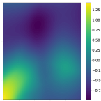
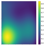
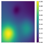
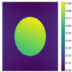
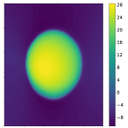
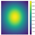
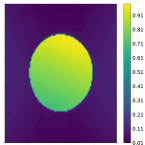
For both $f_{1}$ and $f_{2}$ we can observe that the $\delta$NN-VSKs and VSKs-$f$ behave better than FSK and $\delta$NN, coherently with Proposition 3.1 and Remark 3.1. For the discontinuous function $f_{2}$ the improvement in terms of SSIM of the VSKs-based methods is evident, however, the most relevant result is the one reported in Figure 1. Here we report the reconstructions of the two target functions $f_{1}$ and $f_{2}$ together with the learned scaling functions. Because of the similarity between the targets and the recovered scaling functions, on the one hand, the $\delta$NN-VSKs method supports our theoretical claims and, on the other one, offers the opportunity to automatically define a scaling function for the VSKs.

As future work, we plan to learn simultaneously both the scaling function for VSKs and the optimal sampling locations producing in that way sparse models (see e.g. [13, 14, 15]).

		MSE
	$n$	FSK	$\delta$NN	$\delta$NN-VSKs	VSKs-$f$
$f_{1}$	729	4.2498e-3	2.6381e-5	1.4246e-4	2.4368e-5
	1089	9.8816e-4	1.2737e-5	2.3377e-5	8.2578e-6
	1521	3.8427e-7	1.0050e-5	3.8392e-7	2.7049e-7
$f_{2}$	729	3.7403e-2	4.9117e-3	3.8652e-3	4.5955e-3
	1089	2.1595e-2	3.0441e-3	2.7193e-3	3.0060e-3
	1521	9.2245e-3	2.0504e-3	1.1860e-3	1.3208e-3

Table 1: MAEs for the test functions $f_{1}$ and $f_{2}$.

		SSIM
	$n$	FSK	$\delta$NN	$\delta$NN-VSKs	VSKs-$f$
$f_{1}$	729	0.8712	0.9939	0.9820	0.9943
	1089	0.9533	0.9971	0.9969	0.9980
	1521	0.9997	0.9971	0.9997	0.9999
$f_{2}$	729	0.6118	0.8891	0.9113	0.8901
	1089	0.6072	0.9254	0.9300	0.9482
	1521	0.6676	0.9226	0.9715	0.9633

Table 2: SSIMs for the test functions $f_{1}$ and $f_{2}$.

Figure 1: Top and bottom: results for the function $f_{1}$ and $f_{2}$. Left to right: target function, scaling function, approximation with FSK and $\delta$NN-VSKs.

References

- [1] M. Bozzini, L. Lenarduzzi, M. Rossini, R. Schaback, Interpolation with variably scaled kernels, IMA J. Numer. Anal. 35 (1) (2015) 199–219.
- [2] S. De Marchi, W. Erb, F. Marchetti, E. Perracchione, M. Rossini, Shape-driven interpolation with discontinuous kernels: Error analysis, edge extraction, and applications in magnetic particle imaging, SIAM J. Sci. Comput. 42 (2) (2020) B472–B491.
- [3] E. Perracchione, F. Camattari, A. Volpara, P. Massa, A. M. Massone, M. Piana, Unbiased clean for stix in solar orbiter, Astrophys. J. Suppl. S. 268 (2) (2023).
- [4] F. Della Santa, S. Pieraccini, Discontinuous neural networks and discontinuity learning, J. Comput. Appl. Math. 419 (2023).
- [5] G. E. Fasshauer, M. McCourt, Kernel-based Approximation Methods using MATLAB, World scientific, 2015.
- [6] H. Wendland, Scattered Data Approximation, Cambridge University Press, 2004.
- [7] M. K. Esfahani, S. De Marchi, F. Marchetti, Moving least squares approximation using variably scaled discontinuous weight function, Constr. Math. Anal. 6 (1) (2023) 38–54.
- [8] M. Rossini, Interpolating functions with gradient discontinuities via Variably Scaled Kernels, Dolomites Res. Notes Approx. 17 (2018) 3–14.
- [9] P. Kidger, T. Lyons, Universal approximation with deep narrow networks, Vol. 125, 2020, pp. 2306–2327.
- [10] T. A. Driscoll, B. Fornberg, Interpolation in the limit of increasingly flat radial basis functions, Comput. Math. Appl. 43 (3-5) (2002) 413–422.
- [11] L. Ling, F. Marchetti, A stochastic extended Rippa’s algorithm for LpOCV, Appl. Math. Letters 129 (2022) 107955.
- [12] T. Wenzel, F. Marchetti, E. Perracchione, Data-driven kernel designs for optimized greedy schemes: A machine learning perspective, SIAM J. Sci. Comput. 46 (1) (2024) C101–C126.
- [13] F. Camattari, S. Guastavino, F. Marchetti, M. Piana, E. Perracchione, Classifier-dependent feature selection via greedy methods, Statist. Comput. 34 (151) (2024) 1–12.
- [14] S. De Marchi, R. Schaback, H. Wendland, Near-optimal data-independent point locations for radial basis function interpolation, Adv. Comput. Math. 23 (3) (2005) 317–330.
- [15] T. Wenzel, G. Santin, B. Haasdonk, Analysis of Target Data-Dependent Greedy Kernel Algorithms: Convergence Rates for -, - and -Greedy, Constr. Approx. (2022).