Convergence analysis of the Alternating Anderson-Picard method for nonlinear fixed-point problems

Abstract

Anderson Acceleration (AA) has been widely used to solve nonlinear fixed-point problems due to its rapid convergence. This work focuses on a variant of AA in which multiple Picard iterations are performed between each AA step, referred to as the Alternating Anderson-Picard (AAP) method. Despite introducing more ‘slow’ Picard iterations, this method has been shown to be efficient and even more robust in both linear and nonlinear cases. However, there is a lack of theoretical analysis for AAP in the nonlinear case, which this paper aims to address. We show the equivalence between AAP and a multisecant-GMRES method that uses GMRES to solve a multisecant linear system at each iteration. More interestingly, the incorporation of Picard iterations and AA establishes a deep connection between AAP and the Newton-GMRES method. This connection is evident in terms of the multisecant matrix, the approximate Jacobian inverse, search direction, and optimization gain—an essential factor in the convergence analysis of AA. We show that these terms converge to their corresponding terms in the Newton-GMRES method as the residual approaches zero. Consequently, we build the convergence analysis of AAP. To validate our theoretical findings, numerical examples are provided.

68Q25, 68R10, 68U05

1 Introduction

Fixed-point iterations are one of the cornerstones in scientific computing, formulated by

(1) $$\boldsymbol{x}=g(\boldsymbol{x}),$$

where $\boldsymbol{x}\in\mathbb{R}^{d}$ and $g:\mathbb{R}^{d}\rightarrow\mathbb{R}^{d}$ is assumed to be a continuously differentiable operator in this work. The standard method for solving (1) is the fixed-point iteration, also known as the Picard iteration, noted for its simplicity but also for its potentially slow convergence. This paper concerns an acceleration method for nonlinear fixed-point iterations.

Anderson acceleration (AA), initially introduced in [2] to address partial differential equations, is one of the most popular acceleration schemes. AA is a scheme mixing history points with mixing coefficients computed by solving a least-squares (LS) problem. It can be regarded as a multisecant quasi-Newton method whose approximate Jacobian inverse satisfies a multisecant equation [13]. AA is known for its simplicity and significantly improved convergence performance. It has wide applications in fields such as electronic structure calculations [3, 13], fluid dynamics [22], geometrical optimization [27], and more recently machine learning [15, 38].

The classical AA method takes an AA step in each iteration. There are different variants of AA such as restarted AA [26], type-I AA [13, 39], and EDIIS [7]. Among these alternatives, a simple method that applies AA at periodic intervals rather than every iteration draws our attention. Contrary to the belief that a reduced frequency of AA would degrade performance, this technique has been proven to enhance both the efficiency and robustness of AA. This method was first introduced to address large-scale linear systems within the classical Jacobi fixed-point iteration framework for electronic structure calculations, termed the Alternating Anderson-Jacobi (AAJ) method, in[31], where it has been shown to significantly outperform both the GMRES and Anderson-accelerated Jacobi methods. Subsequently, AAJ was generalized to include preconditioning, known as the Alternating Anderson-Richardson (AAR) method; it outperforms classical preconditioned Krylov solvers in terms of efficiency and scalability [35]. In nonlinear scenarios, [3] uses this strategy for accelerating self-consistent field iterations, and [18] applied a similar strategy on Riemannian optimization. On the theoretical side, [23] provides a convergence analysis of AAR, establishing its equivalence to GMRES. However, no theoretical convergence analysis exists yet for the application of this alternating approach to solve nonlinear fixed-point problems, which is the primary focus of this work.

We consider a specific variant of this periodically alternating method, referred to as AAP, which takes $m$ Picard iterations between each AA step, and takes an AA step to mix all $m+1$ points. We refer to the method AAP($m$) in this paper when the number of Picard iterations $m$ needs to be specified. A detailed description of AAP is given in Algorithm 1. This method takes advantage of the efficiency of AA to improve the convergence, while maintaining the simplicity of the Picard iterations.

Solving (1) is equivalent to finding the root of the residual function:

(2) $$0=f(\boldsymbol{x}):=g(\boldsymbol{x})-\boldsymbol{x}.$$

Newton-type methods are fundamental in this context due to their characteristic fast convergence, achieved by utilizing Jacobian information [24]. One such method, Newton-GMRES [8, 1], iteratively updates the solution by solving the root of the linear approximation of $f$ using GMRES  [20]. In this work, we will study the properties of the AAP method. The core is to establish the equivalence between AAP and a multisecant-GMRES method, which iteratively uses GMRES to find the root of a multisecant linear approximation of $f$. In addition, compared to other variants of AA, the characteristic that all history points used in each AA step are generated by Picard iterations allows AAP capture local information more effectively. Formally, we will show that AAP has a deep connection to the Newton-GMRES method.

This paper is organized as follows. Section 2 details the AAP algorithm and related work. Section 3 demonstrates that, at each global iteration $t$, AAP($m$) implicitly solves a multisecant linear system using the GMRES($m$) method, followed by one additional linearized Picard iteration. Section 4 explores the connection between AAP and the Newton-GMRES method, focusing on the multisecant matrix, the approximate Jacobian inverse, search direction, and optimization gain – an essential factor in the convergence analysis of AA. We show that as the residual approaches zero, these terms converge to their corresponding terms in the Newton-GMRES method. Section 5 presents the convergence analysis of AAP, including a one-step residual bound and the local convergence result. Numerical examples are provided in Section 6. Appendix A discusses an assumption for guaranteeing the convergence of AAP.

1.1 Notation

The vector norm is denoted by $\|\cdot\|$ and refers to the Euclidean norm (2-norm). The matrix norm is also denoted by $\|\cdot\|$ and refers to the induced 2-norm, which is the largest singular value. A sequence of matrices $\boldsymbol{A}_{k}\rightarrow\boldsymbol{A}$ means $\|\boldsymbol{A}_{k}-\boldsymbol{A}\|\rightarrow 0$. In this paper, a sequence of matrices $\boldsymbol{A}_{k}\rightarrow\widetilde{\boldsymbol{A}}_{k}$, where $\widetilde{\boldsymbol{A}}_{k}$ is another sequence of matrices, means $\|\boldsymbol{A}_{k}-\widetilde{\boldsymbol{A}}_{k}\|\rightarrow 0$; we refer to this as the convergence of $\boldsymbol{A}_{k}$ to $\widetilde{\boldsymbol{A}}_{k}$. The Frobenius norm of the matrix is denoted as $\|\cdot\|_{F}$. The identity matrix is denoted by $\boldsymbol{I}$. For better presentation in this paper, $\boldsymbol{A}^{\ell}$ represents a superscript on matrix $\boldsymbol{A}$; $\boldsymbol{A}^{(\ell)}$ refers to the matrix $\boldsymbol{A}$ raised to the power $\ell$. $\boldsymbol{A}^{-1}$ denotes the inverse of matrix $\boldsymbol{A}$. $\boldsymbol{A}^{\dagger}$ denotes the left pseudoinverse of matrix $\boldsymbol{A}$. The $i$th largest singular value of $\boldsymbol{A}$ is denoted as $\sigma_{i}(\boldsymbol{A})$ , and $\sigma_{\text{min}}(\boldsymbol{A})$ is the smallest singular value of $\boldsymbol{A}$. The condition number of $\boldsymbol{A}$ is denoted as $\mathrm{cond}(\boldsymbol{A})$. The subspace spanned by the columns of matrix $\boldsymbol{A}$ is denoted as $\mathrm{span}(\boldsymbol{A})$.

For a given matrix $\boldsymbol{A}$ and vector $\boldsymbol{b}$, the $n$-th Krylov subspace is defined as:

$$\mathcal{K}_{n}(\boldsymbol{A},\boldsymbol{b})=\mathrm{span}\{\boldsymbol{b},\boldsymbol{A}\boldsymbol{b},\boldsymbol{A}^{2}\boldsymbol{b},\ldots,\boldsymbol{A}^{n-1}\boldsymbol{b}\}.$$

Krylov subspaces are shift invariant, i.e., for any $\nu\in\mathbb{R}$, $\mathcal{K}_{n}(\boldsymbol{A}-\nu\boldsymbol{I},\boldsymbol{b})=\mathcal{K}_{n}(\boldsymbol{A},\boldsymbol{b})$. The Generalized Minimal Residual Method (GMRES) is one of the most popular Krylov subspace methods and solves the linear systems $\boldsymbol{A}\boldsymbol{x}=\boldsymbol{b}$ by minimizing the residual within a Krylov subspace at iteration $n$:

$$\min_{\boldsymbol{x}\in\mathcal{K}_{n}(\boldsymbol{A},\boldsymbol{b})}\|\boldsymbol{A}\boldsymbol{x}-\boldsymbol{b}\|.$$

The following assumptions will be used in this paper:

Assumption 1.1.

The following properties are assumed for $g$:

1. $\|g(\boldsymbol{x})-g(\boldsymbol{y})\|\leq\kappa\|\boldsymbol{x}-\boldsymbol{y}\|,\quad\forall\,\,\boldsymbol{x},\boldsymbol{y}\in\mathbb{R}^{d}$ with $\kappa\leq 1$.

2. The Jacobian of $g$, denoted as $g^{\prime}$, is Lipschitz continuous with constant $\gamma>0$,

   $$\|g^{\prime}(\boldsymbol{x})-g^{\prime}(\boldsymbol{y})\|\leq\gamma\|\boldsymbol{x}-\boldsymbol{y}\|.$$

2 Algorithm and related work

This section provides the details of the AAP algorithm, along with the necessary preliminary concepts and assumptions. In addition, existing work on the convergence analysis of AA is discussed.

2.1 The AAP algorithm

At global iteration $t$, AAP first takes $m$ Picard iterations from current iterate $\boldsymbol{x}_{t}$ to generate new points $\{\boldsymbol{x}_{t}^{1},\cdots,\boldsymbol{x}_{t}^{m}\}$ and compute their residuals. AAP next computes the mixing coefficients by solving a constrained LS problem based on the residuals of the history points $\{\boldsymbol{x}_{t},\boldsymbol{x}_{t}^{1},\cdots,\boldsymbol{x}_{t}^{m}\}$, and then updates the iterate to $\boldsymbol{x}_{t+1}$ by mixing the fixed-point values of these points. See Algorithm 1 for details. We denote the mixing coefficients at global iteration $t$ as $\boldsymbol{\alpha}_{t}=\{\alpha_{t}^{0},\alpha_{t}^{1},...,\alpha_{t}^{m}\}\in\mathbb{R}^{m+1}$, and denote the residual $f(\boldsymbol{x}_{t})$ as either $\boldsymbol{f}_{t}$ or $\boldsymbol{f}_{t}^{0}$, depending on the context. When relevant, we refer to this algorithm as AAP($m$), in which $m+1$ Picard iterations are performed in each global iteration.

Algorithm 1 Alternating Anderson-Picard (AAP) Method

1:Initialization: $\boldsymbol{x}_{0}\in\mathbb{R}^{d}$, number of Picard steps $m\leq d$, damping ratio $\beta_{t}\geq 0$

2:for global iteration $t=0$ to $T$ do

3:     /* Step 1: takes Picard iteration to generate $m$ points and compute their residuals */

4:     $\boldsymbol{x}_{t}^{0}\leftarrow\boldsymbol{x}_{t}$

5:     for $\ell=1$ to $m$ do

6:         $\boldsymbol{x}_{t}^{\ell}\leftarrow g(\boldsymbol{x}_{t}^{\ell-1})$

7:         $\boldsymbol{f}_{t}^{\ell-1}\leftarrow\boldsymbol{x}_{t}^{\ell}-\boldsymbol{x}_{t}^{\ell-1}$

8:     end for

9:     $\boldsymbol{f}_{t}^{m}\leftarrow g(\boldsymbol{x}_{t}^{m})-\boldsymbol{x}_{t}^{m}$

10:     /* Step 2: Take one Anderson Acceleration step */

11:     Solve

(3) $$\boldsymbol{\alpha}_{t}\leftarrow\operatorname*{arg\,min}_{\alpha\in\mathbb{R}^{m+1}}\big{\|}\sum_{\ell=0}^{m}\alpha^{\ell}\boldsymbol{f}_{t}^{\ell}\big{\|}^{2}\quad\text{s.t.}\quad\sum_{\ell=0}^{m}\alpha^{\ell}=1$$

12:     Update

(4) $$\boldsymbol{x}_{t+1}\leftarrow(1-\beta_{t})\sum_{\ell=0}^{m}\alpha_{t}^{\ell}\boldsymbol{x}_{t}^{\ell}+\beta_{t}\sum_{\ell=0}^{m}\alpha_{t}^{\ell}g(\boldsymbol{x}_{t}^{\ell})$$

13:end for

Here the damping ratio $\beta_{t}$ balances the weighted average of history points and the weighted average of history residuals, i.e.,

(5) $$\boldsymbol{x}_{t+1}=(1-\beta_{t})\sum_{\ell=0}^{m}\alpha_{t}^{\ell}\boldsymbol{x}_{t}^{\ell}+\beta_{t}\sum_{\ell=0}^{m}\alpha_{t}^{\ell}g(\boldsymbol{x}_{t}^{\ell})=\sum_{\ell=0}^{m}\alpha_{t}^{\ell}\boldsymbol{x}_{t}^{\ell}+\beta_{t}\sum_{\ell=0}^{m}\alpha_{t}^{\ell}\boldsymbol{f}_{t}^{\ell}.$$

Let $\boldsymbol{S}_{t}:=[\boldsymbol{s}_{t}^{0},\dots,\boldsymbol{s}_{t}^{m-1}]\in\mathbb{R}^{d\times m}$ and $\boldsymbol{Y}_{t}:=[\boldsymbol{y}_{t}^{0},\dots,\boldsymbol{y}_{t}^{m-1}]\in\mathbb{R}^{d\times m}$ with $\boldsymbol{s}_{t}^{\ell}=\boldsymbol{x}_{t}^{\ell+1}-\boldsymbol{x}_{t}^{\ell}$ and $\boldsymbol{y}_{t}^{\ell}=\boldsymbol{f}^{\ell+1}_{t}-\boldsymbol{f}^{\ell}_{t}$, for $\ell=0,\dots,m-1$. When $\boldsymbol{Y}_{t}$ is of full column rank, the constrained LS problem (3) can be written as an unconstrained LS problem, i.e.,

(6) $$\boldsymbol{z}_{t}:=\operatorname*{arg\,min}_{\boldsymbol{z}\in\mathbb{R}^{m}}\|\boldsymbol{Y}_{t}\boldsymbol{z}-\boldsymbol{f}_{t}\|^{2}(=\boldsymbol{Y}_{t}^{\dagger}\boldsymbol{f}_{t}),$$

and $\boldsymbol{\alpha}_{t}$ can be recovered from $\boldsymbol{z}_{t}$ by setting $\alpha_{t}^{0}=1+z_{t}^{0}$, $\alpha_{t}^{\ell}=z_{t}^{\ell}-z_{t}^{\ell-1}$ for $0<\ell<m$, and $\alpha_{t}^{m}=-z_{t}^{m-1}$. This transformation leads to an equivalent multisecant quasi-Newton formulation of AAP, which updates $\boldsymbol{x}_{t+1}$ based on an approximate Jacobian inverse $\boldsymbol{H}_{t}$. Specifically,

(7) $$\boldsymbol{x}_{t+1}\leftarrow\boldsymbol{x}_{t}-\boldsymbol{H}_{t}\boldsymbol{f}_{t},$$

(8) $$\begin{aligned} \text{where}\quad\quad&\boldsymbol{H}_{t}\leftarrow-\beta_{t}\boldsymbol{I}+(\boldsymbol{S}_{t}+\beta_{t}\boldsymbol{Y}_{t})(\boldsymbol{Y}_{t}^{T}\boldsymbol{Y}_{t})^{-1}\boldsymbol{Y}_{t}^{T}.\end{aligned}$$

It is straightforward to verify that $\boldsymbol{H}_{t}$ satisfies the inverse multisecant equation $\boldsymbol{H}_{t}\boldsymbol{Y}_{t}=\boldsymbol{S}_{t}$.

The following assumptions regarding the iterations generated by AAP are important for this paper.

Assumption 2.1.

For all $t\geq 0$, both $\boldsymbol{S}_{t}$ and $\boldsymbol{Y}_{t}$ have full column rank.

2.1 is fundamental for all the results presented in this paper and will be assumed without further mention. This assumption is reasonable as we can adaptively adjust $m$ in each global iteration and stop the Picard iterations when the columns of $\boldsymbol{S}_{t}$ or $\boldsymbol{Y}_{t}$ become linearly independent. Alternatively, we can remove the linearly dependent columns directly, though this approach may affect the analysis presented in this paper.

Assumption 2.2 (Uniform Boundedness of $\mathrm{cond}(\boldsymbol{S}_{t})$).

There exist constants $T>0$ and $M>0$ such that $\mathrm{cond}(\boldsymbol{S}_{t})\leq M$ for all $t>T$.

2.2 is a general assumption in the convergence analysis of AA (see Section 2.3). We will show that $\boldsymbol{S}_{t}$ converges to a Krylov matrix in Section 4.2, and discuss this assumption in more detail in Appendix A.

2.2 Multisecant matrices

In this paper, we define the multisecant matrix $\boldsymbol{B}_{t}$ as a matrix that satisfies the multisecant equation $\boldsymbol{B}_{t}\boldsymbol{S}_{t}=\boldsymbol{Y}_{t}$. It follows from $\boldsymbol{s}_{t}^{\ell}=\boldsymbol{x}_{t}^{\ell+1}-\boldsymbol{x}_{t}^{\ell}=\boldsymbol{f}^{\ell}_{t}$ that

(9) $$\boldsymbol{B}_{t}\boldsymbol{S}_{t}=\boldsymbol{Y}_{t},\quad\Longleftrightarrow\quad\boldsymbol{B}_{t}\boldsymbol{f}_{t}^{\ell}=\boldsymbol{f}_{t}^{\ell+1}-\boldsymbol{f}_{t}^{\ell},\quad\forall\,\,0\leq\ell\leq m-1.$$

Furthermore, we define the set

(10) $$\mathbb{B}_{t}:=\{\boldsymbol{B}\in\mathbb{R}^{d\times d}\mid\boldsymbol{B}\boldsymbol{S}_{t}=\boldsymbol{Y}_{t}\}.$$

It is evident that $\mathbb{B}_{t}$ is non-empty and contains invertible matrices under 2.1. For instance, elements of $\mathbb{B}_{t}$ include $\boldsymbol{Y}_{t}\boldsymbol{S}_{t}^{\dagger}$ and $-\boldsymbol{I}+(\boldsymbol{Y}_{t}+\boldsymbol{S}_{t})\boldsymbol{S}_{t}^{\dagger}$. Moreover, an invertible matrix in $\mathbb{B}_{t}$ can be constructed by taking $\boldsymbol{Y}\boldsymbol{S}^{-1}$, where $\boldsymbol{Y}\in\mathbb{R}^{d\times d}$ and $\boldsymbol{S}\in\mathbb{R}^{d\times d}$ are arbitrary invertible matrices with the first $m$ columns being $\boldsymbol{Y}_{t}$ and $\boldsymbol{S}_{t}$, respectively. For any $\boldsymbol{B}_{t}\in\mathbb{B}_{t}$, we call $\widehat{f}_{t}(\boldsymbol{x})=\boldsymbol{B}_{t}(\boldsymbol{x}-\boldsymbol{x}_{t})+f(\boldsymbol{x}_{t})$ a multisecant linear approximation of $f$ at $\boldsymbol{x}_{t}$, which satisfies $\widehat{f}_{t}(\boldsymbol{x}_{t}^{\ell})=f(\boldsymbol{x}_{t}^{\ell})$ for $0\leq\ell\leq m$. At global iteration $t$, this approximation is based on the $m$ Picard iteration points generated in AAP, as seen in the definition of $\mathbb{B}_{t}$.

2.3 Existing convergence analysis of Anderson acceleration

The local convergence rate of AA is established in [36, 19]. Subsequently, [28, 12, 29] demonstrated how AA improves the convergence rate over fixed-point (Picard) iterations. The state-of-the-art convergence bound consists of a linear term and a higher-order term. A simplified result from [29, Theorem 5.1] is given by $\|f(\boldsymbol{x}_{t+1})\|\leq\kappa\theta_{t}\|f(\boldsymbol{x}_{t})\|+c\sqrt{1-\theta_{t}^{2}}\|f(\boldsymbol{x}_{t})\|\sum_{\ell=0}^{m}\|f(\boldsymbol{x}_{t-\ell})\|$ where $\theta_{t}\leq 1$ is called the optimization gain. This result indicates that the local convergence rate of AA, $\kappa\theta_{t}$, is superior to the local convergence rate of the Picard iteration, $\kappa$.

The assumptions to guarantee the convergence of AA include a smoothness condition on $g$ and a uniform boundedness assumption on the coefficients $\boldsymbol{\alpha}$ [36, 12, 29, 25]. Alternatives to the uniform boundedness assumption on $\boldsymbol{\alpha}$ is to assume sufficient linear independence among the columns of $\boldsymbol{Y}_{t}$ [29] and the boundedness of the condition number of $\boldsymbol{S}_{t}$ or $\boldsymbol{Y}_{t}$ [25]. The equivalence between these conditions is discussed in [25]. These conditions are also directly related to the conditioning of the constrained LS problem in AA. In [30], a filtering strategy is proposed to enforce these conditions by removing nearly linearly dependent columns from the LS problem.

An important property of AA is its equivalence to GMRES on linear problems. When $g(\boldsymbol{x})=\boldsymbol{A}\boldsymbol{x}+\boldsymbol{b}$, [37] shows that AA with no truncation solving $\boldsymbol{x}=g(\boldsymbol{x})$ is “essentially equivalent” to GMRES applied to $(\boldsymbol{I}-\boldsymbol{A})\boldsymbol{x}=\boldsymbol{b}$, in the sense that the weighted sum of the history points in each AA step equals the GMRES iterate $\boldsymbol{x}_{t}^{\mathrm{GMRES}}$ and the AA iterate $\boldsymbol{x}_{t+1}^{\mathrm{AA}}=g\left(\boldsymbol{x}_{t}^{\mathrm{GMRES}}\right)$. It is also mentioned in [37] that a “restarted” variant of AA, in which the method proceeds without truncation for $m$ steps and then is restarted, is equivalent to GMRES($m$) applied to $(\boldsymbol{I}-\boldsymbol{A})\boldsymbol{x}=\boldsymbol{b}$ followed by a fixed-point iteration. In [23], the equivalence between Alternating Anderson-Richardson and GMRES is established. For nonlinear problems, AA is closely related to the Nonlinear Generalized Minimal Residual Method (NGMRES) [33]. This work will establish the equivalence bettwen AAP and a multisecant-GMRES method for nonlinear case.

3 Equivalence between AAP and multisecant-GMRES

This section gives the equivalence between AAP and a multisecant-GMRES method. We show that, at global iteration $t$, AAP implicitly solves a multisecant linear system, followed by one additional linearized Picard iteration.

Theorem 3.1 (Equivalence between AAP($m$) and multisecant-GMRES($m$)).

At global iteration $t$, let $\{\boldsymbol{x}_{t}^{\ell}\}_{\ell=0}^{m}$ be generated by AAP($m$), then, for any $\boldsymbol{B}_{t}\in\mathbb{B}_{t}$,

(11) $$\sum_{\ell=0}^{m}\alpha_{t}^{\ell}\boldsymbol{x}_{t}^{\ell}=\boldsymbol{x}_{t}-\widehat{\boldsymbol{p}}_{t},\qquad\text{where}\quad\widehat{\boldsymbol{p}}_{t}=\operatorname*{arg\,min}_{\boldsymbol{p}\in\mathcal{K}_{m}(\boldsymbol{B}_{t},\boldsymbol{f}_{t})}\|\boldsymbol{B}_{t}\boldsymbol{p}-\boldsymbol{f}_{t}\|^{2}.$$

Further, $\boldsymbol{x}_{t+1}=\widehat{g}_{t}(\boldsymbol{x}_{t}-\widehat{\boldsymbol{p}}_{t})$ where $\widehat{g}_{t}(\boldsymbol{x}):=(1-\beta_{t})\boldsymbol{x}+\beta_{t}[(\boldsymbol{I}+\boldsymbol{B}_{t})(\boldsymbol{x}-\boldsymbol{x}_{t})+g(\boldsymbol{x}_{t})]$ is a (damped) linear approximation of $g$.

Proof 3.2.

Let $\boldsymbol{B}_{t}\in\mathbb{B}_{t}$ be any multisecant matrix. By expressing $\boldsymbol{\alpha}$ in terms of $\boldsymbol{z}$ as given in (6),

$$\sum_{\ell=0}^{m}\alpha^{\ell}\boldsymbol{f}_{t}^{\ell} =\boldsymbol{f}_{t}^{0}-z^{0}(\boldsymbol{f}_{t}^{1}-\boldsymbol{f}_{t}^{0})-\cdots-z^{m-1}(\boldsymbol{f}_{t}^{m}-\boldsymbol{f}_{t}^{m-1})=\boldsymbol{f}_{t}-\boldsymbol{Y}_{t}\boldsymbol{z}.$$

From (9), $\boldsymbol{B}_{t}\boldsymbol{f}^{\ell}_{t}=\boldsymbol{f}^{\ell+1}_{t}-\boldsymbol{f}^{\ell}_{t}$ for $0\leq\ell\leq m-1$. This implies that the residual sequence $\{\boldsymbol{f}^{\ell}_{t}\}_{\ell=0}^{m}$ is a Krylov sequence, i.e.,

(12) $$\boldsymbol{f}^{\ell+1}_{t}=(\boldsymbol{I}+\boldsymbol{B}_{t})\boldsymbol{f}^{\ell}_{t}=\cdots=(\boldsymbol{I}+\boldsymbol{B}_{t})^{(\ell+1)}\boldsymbol{f}_{t}\in\mathcal{K}_{\ell+2}(\boldsymbol{I}+\boldsymbol{B}_{t},\boldsymbol{f}_{t}).$$

Then, the columns of $\boldsymbol{Y}_{t}$ take the form $\boldsymbol{y}_{t}^{\ell}=\boldsymbol{f}^{\ell+1}_{t}-\boldsymbol{f}^{\ell}_{t}=(\boldsymbol{I}+\boldsymbol{B}_{t})^{(\ell+1)}\boldsymbol{f}_{t}-(\boldsymbol{I}+\boldsymbol{B}_{t})^{(\ell)}\boldsymbol{f}_{t}=\boldsymbol{B}_{t}(\boldsymbol{I}+\boldsymbol{B}_{t})^{(\ell)}\boldsymbol{f}_{t}$, and thus

$$\mathrm{span}(\boldsymbol{Y}_{t})=\mathrm{span}\{\boldsymbol{y}_{t}^{0},\boldsymbol{y}_{t}^{1},\cdots,\boldsymbol{y}_{t}^{m-1}\}=\boldsymbol{B}_{t}\mathcal{K}_{m}(\boldsymbol{I}+\boldsymbol{B}_{t},\boldsymbol{f}_{t})=\boldsymbol{B}_{t}\mathcal{K}_{m}(\boldsymbol{B}_{t},\boldsymbol{f}_{t}),$$

where the last equality is due to the shift invariance property of the Krylov subspace. Therefore, we have the equivalence between the following three problems:

(13) $$\min_{\boldsymbol{\alpha}\in\mathbb{R}^{m+1},\atop\sum_{\ell=0}^{m}\alpha^{\ell}=1}\|\sum_{\ell=0}^{m}\alpha^{\ell}\boldsymbol{f}_{t}^{\ell}\|^{2}\quad\Leftrightarrow\,\,\min_{\boldsymbol{z}\in\mathbb{R}^{m}}\|\boldsymbol{Y}_{t}\boldsymbol{z}-\boldsymbol{f}_{t}\|^{2}\quad\Leftrightarrow\,\,\min_{\boldsymbol{p}\in\mathcal{K}_{m}(\boldsymbol{B}_{t},\boldsymbol{f}_{t})}\|\boldsymbol{B}_{t}\boldsymbol{p}-\boldsymbol{f}_{t}\|^{2}.$$

It is straightforward to verify that the solutions to each of the problems satisfy

(14) $$\textstyle\sum_{\ell=0}^{m}\alpha_{t}^{\ell}\boldsymbol{f}_{t}^{\ell}=\boldsymbol{f}_{t}-\boldsymbol{Y}_{t}\boldsymbol{z}_{t}=\boldsymbol{f}_{t}-\boldsymbol{B}_{t}\widehat{\boldsymbol{p}}_{t}.$$

As $\boldsymbol{B}_{t}\boldsymbol{S}_{t}=\boldsymbol{Y}_{t}$, we have $\boldsymbol{B}_{t}\widehat{\boldsymbol{p}}_{t}=\boldsymbol{Y}_{t}\boldsymbol{z}_{t}=\boldsymbol{B}_{t}\boldsymbol{S}_{t}\boldsymbol{z}_{t}$ holds for any $\boldsymbol{B}_{t}\in\mathbb{B}_{t}$. Since $\mathbb{B}_{t}$ contains invertible elements, we have $\widehat{\boldsymbol{p}}_{t}=\boldsymbol{S}_{t}\boldsymbol{z}_{t}$. The equivalence between $\boldsymbol{\alpha}_{t}$ and $\boldsymbol{z}_{t}$ then implies $\sum_{\ell=0}^{m}\alpha_{t}^{\ell}\boldsymbol{x}_{t}^{\ell}=\boldsymbol{x}_{t}-\boldsymbol{S}_{t}\boldsymbol{z}_{t}=\boldsymbol{x}_{t}-\widehat{\boldsymbol{p}}_{t}$, and proves (11).

Furthermore, let $\widehat{f}_{t}$ be the multisecant linear approximation of $f$ at $\boldsymbol{x}_{t}$ as $\widehat{f}_{t}(\boldsymbol{x})=\boldsymbol{B}_{t}(\boldsymbol{x}-\boldsymbol{x}_{t})+f(\boldsymbol{x}_{t})$. Then, $\widehat{g}_{t}(\boldsymbol{x})=(1-\beta_{t})\boldsymbol{x}+\beta_{t}(\boldsymbol{x}+\widehat{f}_{t}(\boldsymbol{x}))$. In addition, for all $0\leq\ell\leq m$, $g(\boldsymbol{x}_{t}^{\ell})=\boldsymbol{x}_{t}^{\ell}+f(\boldsymbol{x}_{t}^{\ell})$ and $f(\boldsymbol{x}_{t}^{\ell})=\widehat{f}_{t}(\boldsymbol{x}_{t}^{\ell})$. It follows that

$$\textstyle\sum_{\ell=0}^{m}\alpha_{t}^{\ell}g(\boldsymbol{x}_{t}^{\ell})=\sum_{\ell=0}^{m}\alpha_{t}^{\ell}\boldsymbol{x}_{t}^{\ell}+\sum_{\ell=0}^{m}\alpha_{t}^{\ell}\widehat{f}_{t}(\boldsymbol{x}_{t}^{\ell})=\sum_{\ell=0}^{m}\alpha_{t}^{\ell}\boldsymbol{x}_{t}^{\ell}+\widehat{f}_{t}(\sum_{\ell=0}^{m}\alpha_{t}^{\ell}\boldsymbol{x}_{t}^{\ell}),$$

where the last equation is due to the linearity of $\widehat{f}_{t}$. Finally, we have $\boldsymbol{x}_{t+1}=(1-\beta_{t})\sum_{\ell=0}^{m}\alpha_{t}^{\ell}\boldsymbol{x}_{t}^{\ell}+\beta_{t}[\sum_{\ell=0}^{m}\alpha_{t}^{\ell}\boldsymbol{x}_{t}^{\ell}+\widehat{f}_{t}(\sum_{\ell=0}^{m}\alpha_{t}^{\ell}\boldsymbol{x}_{t}^{\ell})]=\widehat{g}_{t}(\sum_{\ell=0}^{m}\alpha_{t}^{\ell}\boldsymbol{x}_{t}^{\ell})=\widehat{g}_{t}(\boldsymbol{x}_{t}-\widehat{\boldsymbol{p}}_{t})$, which completes the proof.

We have shown that the LS problem (3) in AAP($m$) is equivalent to applying GMRES($m$) to the multisecant linear system $\boldsymbol{B}_{t}\boldsymbol{p}=\boldsymbol{f}_{t}$ for any $\boldsymbol{B}_{t}\in\mathbb{B}_{t}$. We call $\widehat{\boldsymbol{p}}_{t}$ the multisecant-GMRES direction, and $\widehat{\boldsymbol{p}}_{t}$ is equal to $\boldsymbol{S}_{t}\boldsymbol{Y}_{t}^{\dagger}\boldsymbol{f}_{t}$. As shown in Theorem 3.1, the weighted average of the history points equals the multisecant-GMRES update $\boldsymbol{x}_{t}-\widehat{\boldsymbol{p}}_{t}$. The above theorem holds for any $\boldsymbol{B}_{t}\in\mathbb{B}_{t}$ because they generate the same Krylov (residual) subspaces

(15) $$\mathcal{K}_{m}(\boldsymbol{B}_{t},\boldsymbol{f}_{t})=\mathrm{span}(\boldsymbol{S}_{t}),\qquad\boldsymbol{B}_{t}\mathcal{K}_{m}(\boldsymbol{B}_{t},\boldsymbol{f}_{t})=\mathrm{span}(\boldsymbol{Y}_{t}),\quad\forall\,\boldsymbol{B}_{t}\in\mathbb{B}_{t}.$$

We refer to [17] for the properties of matrices that generate the same Krylov residual spaces.

The equivalence between AAP and multisecant-GMRES resembles the one given in [37] for linear $g$. A similar result was also mentioned for a restarted variant of AA applied on gradient descent [26]. The equivalence between other variants of AA and the multisecant methods is discussed in [14].

Let us briefly take a closer look at the damping ratio. To that end, we define the multisecant-GMRES residual at iteration $t$ as $\widehat{\boldsymbol{r}}_{t}$. According to the equivalence between the three minimization problems in (13), we have

(16) $$\widehat{\boldsymbol{r}}_{t}=\boldsymbol{B}_{t}\widehat{\boldsymbol{p}}_{t}-\boldsymbol{f}_{t}=\boldsymbol{Y}_{t}\boldsymbol{z}_{t}-\boldsymbol{f}_{t}=-\sum_{\ell=0}^{m}\alpha_{t}^{\ell}\boldsymbol{f}_{t}^{\ell}.$$

The following corollary shows that the damping ratio acts as a stepsize parameter in the direction of the residual.

Corollary 3.3.

The iterate $\boldsymbol{x}_{t+1}$ generated from (4) in AAP satisfies

(17) $$\boldsymbol{x}_{t+1}=\boldsymbol{x}_{t}-\widehat{\boldsymbol{p}}_{t}-\beta_{t}\widehat{\boldsymbol{r}}_{t}.$$

Proof 3.4.

The result follows from $\boldsymbol{x}_{t+1}=\sum_{\ell=0}^{m}\alpha_{t}^{\ell}\boldsymbol{x}_{t}^{\ell}+\beta_{t}\sum_{\ell=0}^{m}\alpha_{t}^{\ell}\boldsymbol{f}_{t}^{\ell}=\boldsymbol{x}_{t}-\widehat{\boldsymbol{p}}_{t}-\beta_{t}\widehat{\boldsymbol{r}}_{t}.$

When $\beta_{t}$ satisfies $\|\boldsymbol{I}-\beta_{t}\boldsymbol{B}_{t}\|\leq 1$, the “damped” direction $\widehat{\boldsymbol{p}}_{t}+\beta_{t}\widehat{\boldsymbol{r}}_{t}$ could be a better solution to the multisecant linear system $\boldsymbol{B}_{t}\boldsymbol{p}=\boldsymbol{f}_{t}$ than the original direction $\widehat{\boldsymbol{p}}_{t}$. Indeed, in this case, $\|\boldsymbol{B}_{t}(\widehat{\boldsymbol{p}}_{t}+\beta_{t}\widehat{\boldsymbol{r}}_{t})-\boldsymbol{f}_{t}\|=\|(\boldsymbol{I}-\beta_{t}\boldsymbol{B}_{t})(\boldsymbol{B}_{t}\widehat{\boldsymbol{p}}_{t}-\boldsymbol{f}_{t})\|\leq\|\boldsymbol{B}_{t}\widehat{\boldsymbol{p}}_{t}-\boldsymbol{f}_{t}\|$.

4 Connection Between AAP and Newton-GMRES

Newton’s method finds the roots of a nonlinear function $f(\boldsymbol{x})$ by using its Jacobian information. At iteration $t$, a linear approximation of $f$ at $\boldsymbol{x}_{t}$ is given by

(18) $$f(\boldsymbol{x})\approx\boldsymbol{J}_{t}(\boldsymbol{x}-\boldsymbol{x}_{t})+f(\boldsymbol{x}_{t}),$$

where $\boldsymbol{J}_{t}:=f^{\prime}(\boldsymbol{x}_{t})$ is the Jacobian of $f$ at $\boldsymbol{x}_{t}$. The Newton-GMRES($m$) method is a variant of the inexact-Newton method that uses GMRES($m$) to approximately solve this linearized system for a search direction $\boldsymbol{p}^{\textup{N}}_{t}$ at each iteration as follows

(19) $$\boldsymbol{x}_{t+1}:=\boldsymbol{x}_{t}-\boldsymbol{p}^{\textup{N}}_{t}\quad\text{with}\quad\boldsymbol{p}^{\textup{N}}_{t}:=\operatorname*{arg\,min}_{\boldsymbol{p}\in\mathcal{K}_{m}(\boldsymbol{J}_{t},\boldsymbol{f}_{t})}\|\boldsymbol{J}_{t}\boldsymbol{p}-\boldsymbol{f}_{t}\|.$$

However, the Jacobian is not always available or easy to compute directly.

As shown in Corollary 3.3, at iteration $\boldsymbol{x}_{t}$, the search direction given by AAP is equivalent to the multisecant-GMRES direction based on $\boldsymbol{B}_{t}\in\mathbb{B}_{t}$ with an additional damping term. In this section, we establish the connection between AAP and the Newton-GMRES method by showing that, (i) when the residual $\|\boldsymbol{f}_{t}\|$ goes to zero as $t\to\infty$, the distance between the set of multisecant matrix $\mathbb{B}_{t}$ given by AAP and the Jacobian matrix $\boldsymbol{J}_{t}$ converges to zero (Section 4.1), (ii) the matrices $\boldsymbol{S}_{t}$, $\boldsymbol{Y}_{t}$, and $\boldsymbol{H}_{t}$ constructed by AAP converge respectively to their counterparts in the Newton-GMRES method (Section 4.2), and (iii) the optimization gain $\theta_{t}$ in AAP converges to an analogous quantities in Newton-GMRES (Section 4.3).

One of the key properties of AAP that enables the analysis in this section is the $m$ Picard iteration steps taken in a global iteration. The Picard iteration steps often progress more conservatively than the acceleration step. Therefore, the multisecant matrix given by these history points could be a good approximation to the local Jacobian $\boldsymbol{J}_{t}$. In fact, the following lemma provides bounds on the Picard iteration updates and residuals, which are essential in the analysis in this section.

Lemma 4.1.

Under 1.1(a), at global iteration $t$ of AAP, for all $0\leq\ell\leq m$,

$$\|\boldsymbol{f}^{\ell}_{t}\|\leq\|\boldsymbol{f}_{t}\|,\quad\text{and}\quad\|\boldsymbol{x}^{\ell}_{t}-\boldsymbol{x}_{t}\|\leq\ell\|\boldsymbol{f}_{t}\|.$$

Proof 4.2.

Since $\boldsymbol{x}_{t}^{\ell}=g(\boldsymbol{x}_{t}^{\ell-1})$ and $\boldsymbol{x}_{t}^{0}=\boldsymbol{x}_{t}$, we have $\boldsymbol{x}_{t}^{\ell}=\boldsymbol{x}_{t}^{\ell-1}+f(\boldsymbol{x}_{t}^{\ell-1})$ and thus $\|\boldsymbol{x}_{t}^{\ell}-\boldsymbol{x}_{t}\|=\|\sum_{i=0}^{\ell-1}f(\boldsymbol{x}_{t}^{i})\|\leq\sum_{i=0}^{\ell-1}\|f(\boldsymbol{x}_{t}^{i})\|$. The non-expansive property of $g$ gives that, for $i=1,\dots,\ell$,

$$\|f(\boldsymbol{x}_{t}^{i})\|=\|g(\boldsymbol{x}_{t}^{i})-\boldsymbol{x}_{t}^{i}\|=\|g(\boldsymbol{x}_{t}^{i})-g(\boldsymbol{x}_{t}^{i-1})\|\leq\kappa\|\boldsymbol{x}_{t}^{i}-\boldsymbol{x}_{t}^{i-1}\|=\kappa\|f(\boldsymbol{x}_{t}^{i-1})\|.$$

Since $\kappa\leq 1$, $\|\boldsymbol{f}^{\ell}_{t}\|\leq\|\boldsymbol{f}_{t}\|$ and $\|\boldsymbol{x}_{t}^{\ell}-\boldsymbol{x}_{t}\|\leq\sum_{i=0}^{\ell-1}\|f(\boldsymbol{x}_{t})\|\leq\ell\|\boldsymbol{f}_{t}\|$.

Another useful technique in the following analysis is the fundamental theorem for line integrals, i.e.,

(20) $$\textstyle f(\boldsymbol{y})-f(\boldsymbol{x})=\int_{0}^{1}f^{\prime}(\boldsymbol{x}+r(\boldsymbol{y}-\boldsymbol{x}))(\boldsymbol{y}-\boldsymbol{x})\,\mathrm{d}r.$$

With these results, we show in the following subsections that, as the AAP residual $\boldsymbol{f}_{t}$ approaches zero, $\boldsymbol{B}_{t}$, $\boldsymbol{S}_{t}$, $\boldsymbol{Y}_{t}$, $\boldsymbol{H}_{t}$, and $\theta_{t}$ in AAP converge to their counterparts in Newton-GMRES.

4.1 Convergence of the multisecant matrix

We start the analysis with showing that the distance between the set of multisecant matrices $\mathbb{B}_{t}$ generated by AAP and the Jacobian $\boldsymbol{J}_{t}$ goes to zero provided that the residual approaches zero as $t\to\infty$. Here, the distance between $\mathbb{B}_{t}$ and $\boldsymbol{J}_{t}$ is defined as the norm of

(21) $$\boldsymbol{E}_{t}:=\boldsymbol{B}_{t}^{*}-\boldsymbol{J}_{t},\quad\text{where}\quad\boldsymbol{B}_{t}^{*}:=\operatorname*{arg\,min}_{\boldsymbol{B}\in\mathbb{B}_{t}}\|\boldsymbol{B}-\boldsymbol{J}_{t}\|.$$

Because $\boldsymbol{S}_{t}$ is full column rank, the minimal-norm property [37] gives

(22) $$\boldsymbol{E}_{t}=(\boldsymbol{J}_{t}\boldsymbol{S}_{t}-\boldsymbol{Y}_{t})\boldsymbol{S}_{t}^{\dagger}.$$

Note that $\boldsymbol{J}_{t}+\boldsymbol{E}_{t}=\boldsymbol{B}_{t}^{*}\in\mathbb{B}_{t}$. In addition, when $g$ is linear, $\boldsymbol{J}_{t}$ satisfies $\boldsymbol{J}_{t}\boldsymbol{S}_{t}=\boldsymbol{Y}_{t}$ and thus $\|\boldsymbol{E}_{t}\|=0$. An upper bound on $\|\boldsymbol{E}_{t}\|$ for the nonlinear case is provided in the following theorem.

Theorem 4.3.

Under 1.1,

(23) $$\|\boldsymbol{E}_{t}\|\leq\gamma m^{\frac{3}{2}}\mathrm{cond}(\boldsymbol{S}_{t})\|\boldsymbol{f}_{t}\|.$$

Furthermore, if 2.2 holds, then

(24) $$\|\boldsymbol{E}_{t}\|\leq C_{E}\|\boldsymbol{f}_{t}\|,\quad\quad\forall\,\,t>T,$$

where $C_{E}>0$ is a constant that is independent of $t$.

Proof 4.4.

It follows from (22) that

$$\|\boldsymbol{E}_{t}\|\leq\|\boldsymbol{Y}_{t}-\boldsymbol{J}_{t}\boldsymbol{S}_{t}\|\|\boldsymbol{S}_{t}^{\dagger}\|.$$

Let $\boldsymbol{Y}_{t}-\boldsymbol{J}_{t}\boldsymbol{S}_{t}=[\boldsymbol{v}^{0},\boldsymbol{v}^{1},\dots,\boldsymbol{v}^{m-1}]\in\mathbb{R}^{d\times m}$. For $0\leq\ell\leq m-1$,

$$\boldsymbol{v}^{\ell}=\boldsymbol{y}^{\ell}-\boldsymbol{J}_{t}\boldsymbol{s}^{\ell}=f(\boldsymbol{x}_{t}^{\ell+1})-f(\boldsymbol{x}_{t}^{\ell})-f^{\prime}(\boldsymbol{x}_{t})(\boldsymbol{x}_{t}^{\ell+1}-\boldsymbol{x}_{t}^{\ell}).$$

By using (20) and $\boldsymbol{s}_{t}^{\ell}=\boldsymbol{x}_{t}^{\ell+1}-\boldsymbol{x}_{t}^{\ell}=\boldsymbol{f}_{t}^{\ell}$,

$$\boldsymbol{v}^{\ell} =\int_{0}^{1}f^{\prime}(\boldsymbol{x}^{\ell}_{t}+r\boldsymbol{f}^{\ell}_{t})\boldsymbol{f}^{\ell}_{t}\,\mathrm{d}r-f^{\prime}(\boldsymbol{x}_{t})\boldsymbol{f}^{\ell}_{t}=\int_{0}^{1}[f^{\prime}(\boldsymbol{x}^{\ell}_{t}+r\boldsymbol{f}^{\ell}_{t})-f^{\prime}(\boldsymbol{x}_{t})]\boldsymbol{f}^{\ell}_{t}\,\mathrm{d}r.$$

Applying $f^{\prime}(\boldsymbol{x})=g^{\prime}(\boldsymbol{x})-\boldsymbol{I}$ and the Lipschitz continuity of $g^{\prime}$ gives, for $r\in[0,1]$,

$$\|f^{\prime}(\boldsymbol{x}^{\ell}_{t}+r\boldsymbol{f}^{\ell}_{t})-f^{\prime}(\boldsymbol{x}_{t})\|\leq\gamma\|\boldsymbol{x}^{\ell}_{t}+r\boldsymbol{f}^{\ell}_{t}-\boldsymbol{x}_{t}\|\leq\gamma(\|\boldsymbol{x}^{\ell}_{t}-\boldsymbol{x}_{t}\|+\|\boldsymbol{f}^{\ell}_{t}\|).$$

By Lemma 4.1, $\|\boldsymbol{x}^{\ell}_{t}-\boldsymbol{x}_{t}\|+\|\boldsymbol{f}^{\ell}_{t}\|\leq(\ell+1)\|\boldsymbol{f}_{t}\|\leq\gamma m\|\boldsymbol{f}_{t}\|$ as $\ell<m$, which leads to

(25) $$\|\boldsymbol{v}^{\ell}\|\leq\int_{0}^{1}\|f^{\prime}(\boldsymbol{x}^{\ell}_{t}+r\boldsymbol{f}^{\ell}_{t})-f^{\prime}(\boldsymbol{x}_{t})\|\|\boldsymbol{f}^{\ell}_{t}\|\,\mathrm{d}r\leq\gamma m\|\boldsymbol{f}_{t}\|\|\boldsymbol{s}_{t}^{\ell}\|.$$

Using the matrix norm inequality $\|\cdot\|\leq\|\cdot\|_{F}$,

$$\|\boldsymbol{J}_{t}\boldsymbol{S}_{t}-\boldsymbol{Y}_{t}\|\leq\|\boldsymbol{J}_{t}\boldsymbol{S}_{t}-\boldsymbol{Y}_{t}\|_{F}=\sqrt{\sum_{\ell}\|\boldsymbol{v}^{\ell}\|^{2}}\leq\gamma m\|\boldsymbol{f}_{t}\|\sqrt{\sum_{\ell}\|\boldsymbol{s}_{t}^{\ell}\|^{2}}=\gamma m\|\boldsymbol{f}_{t}\|\|\boldsymbol{S}_{t}\|_{F}.$$

Since $\boldsymbol{S}_{t}$ has full column rank and $\|\boldsymbol{S}_{t}\|_{F}\leq\sqrt{m}\|\boldsymbol{S}_{t}\|$, it follows that

$$\|\boldsymbol{E}_{t}\|\leq\sqrt{m}\gamma m\|\boldsymbol{f}_{t}\|\|\boldsymbol{S}_{t}\|\|\boldsymbol{S}_{t}^{\dagger}\|=\gamma m^{\frac{3}{2}}\|\boldsymbol{f}_{t}\|\mathrm{cond}(\boldsymbol{S}_{t}).$$

The second claim is then a direct consequence of 2.2.

The bound given in (24) shows that $\|\boldsymbol{E}_{t}\|\leq\mathcal{O}(\|\boldsymbol{f}_{t}\|)$, which leads to the following convergence result.

Corollary 4.5.

Under Assumptions 1.1 and 2.2, suppose that $\boldsymbol{f}_{t}\to 0$ as $t\to\infty$, then, as $t\to\infty$,

$$\boldsymbol{E}_{t}\rightarrow 0\quad\text{and}\quad\boldsymbol{B}_{t}^{*}\rightarrow\boldsymbol{J}_{t},$$

where $\boldsymbol{B}_{t}^{*}\in\mathbb{B}_{t}$ is defined in (21).

The convergence of $\boldsymbol{B}_{t}$ to $\boldsymbol{J}_{t}$ suggests that the multisecant direction $\widehat{\boldsymbol{p}}_{t}$ could converge to the Newton-GMRES direction ${\boldsymbol{p}}^{\textup{N}}_{t}:=\operatorname*{arg\,min}_{\boldsymbol{p}\in\mathcal{K}_{m}(\boldsymbol{J}_{t},\boldsymbol{f}_{t})}\|\boldsymbol{J}_{t}\boldsymbol{p}-\boldsymbol{f}_{t}\|$, which we prove later in Corollary 4.10.

4.2 Limits of $\boldsymbol{S}_{t}$, $\boldsymbol{Y}_{t}$, and $\boldsymbol{H}_{t}$

In this section, we establish the limits of $\boldsymbol{S}_{t}$ and $\boldsymbol{Y}_{t}$ as $t\to\infty$ under the assumption that $\boldsymbol{f}_{t}$ approaches zero. These limits are related to a Krylov matrix spanned by $g^{\prime}(\boldsymbol{x}_{t})$ and $\boldsymbol{f}_{t}$, which further implies the convergence of the approximate Jacobian inverse $\boldsymbol{H}_{t}$ of AAP defined in (8).

We first review the Newton-GMRES method. At iteration $\boldsymbol{x}_{t}$, the Krylov matrix associated with $\mathcal{K}_{m}(\boldsymbol{J}_{t},\boldsymbol{f}_{t})$ can be written as

(26) $$\boldsymbol{F}_{t}:=[\boldsymbol{f}_{t},\boldsymbol{J}_{t}^{(1)}\boldsymbol{f}_{t},\boldsymbol{J}_{t}^{(2)}\boldsymbol{f}_{t},\cdots,\boldsymbol{J}_{t}^{(m-1)}\boldsymbol{f}_{t}]\in\mathbb{R}^{d\times m}.$$

The Newton-GMRES direction $\boldsymbol{p}^{\textup{N}}_{t}:=\operatorname*{arg\,min}_{\boldsymbol{p}\in\mathcal{K}_{m}(\boldsymbol{J}_{t},\boldsymbol{f}_{t})}\|\boldsymbol{J}_{t}\boldsymbol{p}-\boldsymbol{f}_{t}\|$ satisfies $\boldsymbol{J}_{t}\boldsymbol{p}^{\textup{N}}_{t}$$=\mathcal{P}_{\boldsymbol{J}_{t}\boldsymbol{F}_{t}}(\boldsymbol{f}_{t})$ where $\mathcal{P}_{\boldsymbol{A}}=\boldsymbol{A}\boldsymbol{A}^{\dagger}$ denotes the orthogonal projection onto the subspace spanned by the columns of $\boldsymbol{A}$. Define

(27) $$\boldsymbol{G}_{t}:=[\boldsymbol{f}_{t},g^{\prime}(\boldsymbol{x}_{t})^{(1)}\boldsymbol{f}_{t},g^{\prime}(\boldsymbol{x}_{t})^{(2)}\boldsymbol{f}_{t},\cdots,g^{\prime}(\boldsymbol{x}_{t})^{(m-1)}\boldsymbol{f}_{t}]\in\mathbb{R}^{d\times m}.$$

Since $g^{\prime}(\boldsymbol{x}_{t})=\boldsymbol{I}+\boldsymbol{J}_{t}$, the shift invariance of the Krylov subspace leads to $\mathcal{P}_{\boldsymbol{G}_{t}}=\mathcal{P}_{\boldsymbol{F}_{t}}$. Therefore, $\mathcal{P}_{\boldsymbol{J}_{t}\boldsymbol{G}_{t}}=\mathcal{P}_{\boldsymbol{J}_{t}\boldsymbol{F}_{t}}$. If $\boldsymbol{J}_{t}$ is invertible, we have

(28) $$\boldsymbol{p}^{\textup{N}}_{t}=\boldsymbol{J}_{t}^{-1}\mathcal{P}_{\boldsymbol{J}_{t}\boldsymbol{G}_{t}}(\boldsymbol{f}_{t}).$$

We refer to $\boldsymbol{J}_{t}^{-1}\mathcal{P}_{\boldsymbol{J}_{t}\boldsymbol{G}_{t}}$ as the Newton-GMRES update operator.

As shown in (12), the AAP residuals $\{\boldsymbol{f}_{t}^{\ell}\}_{\ell=0}^{m-1}$ form a basis of the Krylov subspace $\mathcal{K}_{m}(\boldsymbol{B}_{t},\boldsymbol{f}_{t})$ as $\boldsymbol{f}_{t}^{\ell}=(\boldsymbol{I}+\boldsymbol{B}_{t})^{(\ell)}\boldsymbol{f}_{t}$. Therefore,

$$\boldsymbol{S}_{t}=[\boldsymbol{f}_{t}^{0},\boldsymbol{f}_{t}^{1},\cdots,\boldsymbol{f}_{t}^{m-1}]=[\boldsymbol{f}_{t},(\boldsymbol{I}+\boldsymbol{B}_{t})^{(1)}\boldsymbol{f}_{t},(\boldsymbol{I}+\boldsymbol{B}_{t})^{(2)}\boldsymbol{f}_{t},\cdots,(\boldsymbol{I}+\boldsymbol{B}_{t})^{(m-1)}\boldsymbol{f}_{t}]$$

is a Krylov matrix associated with $\boldsymbol{I}+\boldsymbol{B}_{t}$ and $\boldsymbol{f}_{t}$. As $\boldsymbol{f}_{t}$ approaches zero, the matrices $\boldsymbol{S}_{t}$, $\boldsymbol{Y}_{t}$, and $\boldsymbol{G}_{t}$ all approach zero. Further, the following lemma gives estimates of the distances between $\boldsymbol{S}_{t}$, $\boldsymbol{Y}_{t}$ and their Newton-GMRES counterparts.

Lemma 4.6.

Under Assumption 1.1,

(29) $$\|\boldsymbol{S}_{t}-\boldsymbol{G}_{t}\|\leq\gamma m^{\frac{5}{2}}\|\boldsymbol{f}_{t}\|^{2}\qquad\text{and}\qquad\|\boldsymbol{Y}_{t}-\boldsymbol{J}_{t}\,\boldsymbol{G}_{t}\|\leq 2\gamma m^{\frac{5}{2}}\|\boldsymbol{f}_{t}\|^{2}.$$

Proof 4.7.

For a better presentation, we omit the subscript $t$ in this proof unless necessary. Note that $\boldsymbol{x}^{0}=\boldsymbol{x}_{t}$ is the starting point for the Picard iterations at the global iteration $t$, and $\boldsymbol{f}^{\ell}=f(\boldsymbol{x}_{t}^{\ell})$ for all $0\leq\ell\leq m-1$.

We first define $\boldsymbol{\Delta}_{t}=\boldsymbol{G}_{t}-\boldsymbol{S}_{t}$ and write $\boldsymbol{\Delta}_{t}=[\boldsymbol{\epsilon}^{0},\boldsymbol{\epsilon}^{1},\boldsymbol{\epsilon}^{2},\cdots,\boldsymbol{\epsilon}^{m-1}]$. By the definitions of $\boldsymbol{G}_{t}$ and $\boldsymbol{S}_{t}$, $\boldsymbol{\epsilon}^{0}=0$ and $\boldsymbol{\epsilon}^{\ell}=\boldsymbol{f}^{\ell}-g^{\prime}(\boldsymbol{x}_{t})^{(\ell)}\boldsymbol{f}_{t}$ for $\ell=0,\dots,m-1$. We next estimate $\boldsymbol{\epsilon}^{\ell}$. By (20), $f(\boldsymbol{x}^{\ell})-f(\boldsymbol{x}^{\ell-1})=\int_{0}^{1}f^{\prime}(\boldsymbol{x}^{\ell-1}+r\boldsymbol{f}^{\ell-1})\boldsymbol{f}^{\ell-1}\,\mathrm{d}r$ as $\boldsymbol{x}^{\ell}-\boldsymbol{x}^{\ell-1}=\boldsymbol{f}^{\ell}$. Thus,

$$\boldsymbol{f}^{\ell}=f(\boldsymbol{x}^{\ell}) \textstyle=\int_{0}^{1}[\boldsymbol{I}+f^{\prime}(\boldsymbol{x}^{\ell-1}+r\boldsymbol{f}^{\ell-1})]\boldsymbol{f}^{\ell-1}\,\mathrm{d}r$$

$$\textstyle=\int_{0}^{1}g^{\prime}(\boldsymbol{x}^{\ell-1}+r\boldsymbol{f}^{\ell-1})\boldsymbol{f}^{\ell-1}\,\mathrm{d}r$$

$$\textstyle=g^{\prime}(\boldsymbol{x}_{t})\boldsymbol{f}^{\ell-1}+\int_{0}^{1}[g^{\prime}(\boldsymbol{x}^{\ell-1}+r\boldsymbol{f}^{\ell-1})-g^{\prime}(\boldsymbol{x}_{t})]\boldsymbol{f}^{\ell-1}\,\mathrm{d}r$$

$$=\boldsymbol{K}\boldsymbol{f}^{\ell-1}+\boldsymbol{v}^{\ell-1},$$

where $\boldsymbol{K}:=g^{\prime}(\boldsymbol{x}_{t})$ and $\boldsymbol{v}^{\ell-1}:=\int_{0}^{1}\left[g^{\prime}(\boldsymbol{x}^{\ell-1}+r\boldsymbol{f}^{\ell-1})-g^{\prime}(\boldsymbol{x}_{t})\right]\boldsymbol{f}^{\ell-1}\,\mathrm{d}r$. Applying this relation iteratively gives $\boldsymbol{f}^{\ell}=\boldsymbol{K}^{(\ell)}\boldsymbol{f}_{t}+\sum_{i=0}^{\ell-1}\boldsymbol{K}^{(i)}\boldsymbol{v}^{\ell-1-i}$. Therefore, $\boldsymbol{\epsilon}^{\ell}=\sum_{i=0}^{\ell-1}\boldsymbol{K}^{(i)}\boldsymbol{v}^{\ell-1-i}$. Furthermore, under Assumption 1.1, $\|\boldsymbol{K}\|\leq\kappa\leq 1$ and

$$\|\boldsymbol{v}^{\ell-1}\|\leq\gamma\|\boldsymbol{x}^{\ell-1}+r\boldsymbol{f}^{\ell-1}-\boldsymbol{x}_{t}\|\|\boldsymbol{f}^{\ell-1}\|\leq\gamma\ell\|\boldsymbol{f}_{t}\|\|\boldsymbol{f}^{\ell-1}\|\leq m\gamma\|\boldsymbol{f}_{t}\|^{2},$$

where the second inequality follows from Lemma 4.1 and $0\leq r\leq 1$. Then,

$$\textstyle\|\boldsymbol{\epsilon}^{\ell}\|=\sum_{i=0}^{\ell-1}\boldsymbol{K}^{(i)}\boldsymbol{v}^{\ell-1-i}\leq\sum_{i=0}^{\ell-1}\|\boldsymbol{v}^{\ell-1-i}\|\leq\ell(m\gamma\|\boldsymbol{f}_{t}\|^{2})\leq m^{2}\gamma\|\boldsymbol{f}_{t}\|^{2}.$$

Therefore,

(30) $$\textstyle\|\boldsymbol{S}_{t}-\boldsymbol{G}_{t}\|=\|\boldsymbol{\Delta}_{t}\|\leq\|\boldsymbol{\Delta}_{t}\|_{F}=\sqrt{\sum_{i=0}^{m-1}\|\boldsymbol{\epsilon}^{i}\|^{2}}\leq\gamma m^{\frac{5}{2}}\|\boldsymbol{f}_{t}\|^{2}.$$

To estimate $\|\boldsymbol{Y}_{t}-\boldsymbol{J}_{t}\boldsymbol{G}_{t}\|$, we use the relations established above and write the $\ell$-th column of $\boldsymbol{Y}_{t}$ as

$$\boldsymbol{y}_{t}^{\ell}=\boldsymbol{f}^{\ell+1}-\boldsymbol{f}^{\ell}=\boldsymbol{K}^{(\ell+1)}\boldsymbol{f}_{t}+\boldsymbol{\epsilon}^{\ell+1}-\boldsymbol{K}^{(\ell)}\boldsymbol{f}_{t}-\boldsymbol{\epsilon}^{\ell}=\boldsymbol{J}_{t}\boldsymbol{K}^{(\ell)}\boldsymbol{f}_{t}+\boldsymbol{\epsilon}^{\ell+1}-\boldsymbol{\epsilon}^{\ell},$$

where the last equality is due to $\boldsymbol{K}=g^{\prime}(\boldsymbol{x}_{t})=\boldsymbol{I}+f^{\prime}(\boldsymbol{x}_{t})=\boldsymbol{I}+\boldsymbol{J}_{t}$. Then, we write $\boldsymbol{Y}_{t}=\boldsymbol{J}_{t}\boldsymbol{G}_{t}+\widetilde{\boldsymbol{\Delta}}_{t}-\boldsymbol{\Delta}_{t}$ where $\widetilde{\boldsymbol{\Delta}}_{t}:=[\boldsymbol{\epsilon}^{1},\boldsymbol{\epsilon}^{2},\boldsymbol{\epsilon}^{3},\cdots,\boldsymbol{\epsilon}^{m}]\in\mathbb{R}^{d\times m}$. Following a similar approach as above, one can obtain $\|\widetilde{\boldsymbol{\Delta}}_{t}\|\leq\gamma m^{\frac{5}{2}}\|\boldsymbol{f}_{t}\|^{2}$, and thus

(31) $$\left\|\boldsymbol{Y}_{t}-\boldsymbol{J}_{t}\boldsymbol{G}_{t}\right\|\leq\|\widetilde{\boldsymbol{\Delta}}_{t}\|+\|\boldsymbol{\Delta}_{t}\|\leq 2\gamma m^{\frac{5}{2}}\|\boldsymbol{f}_{t}\|^{2}.$$

When $\boldsymbol{f}_{t}$ approaches 0, despite $\boldsymbol{S}_{t}$ and $\boldsymbol{Y}_{t}$ converging to 0, the above lemma shows that $\frac{1}{\|\boldsymbol{f}_{t}\|}\boldsymbol{S}_{t}\rightarrow\frac{1}{\|\boldsymbol{f}_{t}\|}\boldsymbol{G}_{t}$ and $\frac{1}{\|\boldsymbol{f}_{t}\|}\boldsymbol{Y}_{t}\rightarrow\frac{1}{\|\boldsymbol{f}_{t}\|}\boldsymbol{J}_{t}\boldsymbol{G}_{t}$. We note that, when $g$ is linear, i.e., $\gamma=0$, for all $t$,

(32) $$\boldsymbol{S}_{t}=\boldsymbol{G}_{t},\qquad\text{and}\qquad\boldsymbol{Y}_{t}=\boldsymbol{J}_{t}\boldsymbol{G}_{t}.$$

Now we are ready to give the convergence of the approximate Jacobian inverse $\boldsymbol{H}_{t}$ in AAP. As given in (8), $\boldsymbol{H}_{t}=\boldsymbol{S}_{t}\boldsymbol{Y}_{t}^{\dagger}-\beta_{t}(\boldsymbol{I}-\mathcal{P}_{\boldsymbol{Y}_{t}})$ where $\beta_{t}$ is the damping ratio. The definitions of $\widehat{\boldsymbol{p}}_{t}$ and $\widehat{\boldsymbol{r}}_{t}$ in (11) and (16) lead to $\widehat{\boldsymbol{p}}_{t}=\boldsymbol{S}_{t}\boldsymbol{Y}_{t}^{\dagger}\boldsymbol{f}_{t}$ and $\widehat{\boldsymbol{r}}_{t}=-\beta_{t}(\boldsymbol{I}-\mathcal{P}_{\boldsymbol{Y}_{t}})\boldsymbol{f}_{t}$, respectively. Thus, $\boldsymbol{S}_{t}\boldsymbol{Y}_{t}^{\dagger}$ corresponds to the multisecant-GMRES update operator, and $\boldsymbol{I}-\mathcal{P}_{\boldsymbol{Y}_{t}}$ corresponds to the extra linearized fixed-point iteration in AAP. The following corollary gives the convergence of $\boldsymbol{S}_{t}\boldsymbol{Y}_{t}^{\dagger}$ to the Newton-GMRES update operator defined in (28), as well as the convergence of $\boldsymbol{H}_{t}$.

Assumption 4.1.

There exist constants $T>0$ and $M>0$ such that, for all $t\geq T$, $\boldsymbol{J}_{t}$ is invertible, $\sigma_{\min}(\boldsymbol{Y}_{t})\geq M\|\boldsymbol{f}_{t}\|$, and $\boldsymbol{J}_{t}\,\boldsymbol{G}_{t}$ has full column rank.

Theorem 4.8.

Under Assumptions 1.1 and 4.1, when $\boldsymbol{f}_{t}$ goes to 0,

(33) $$\boldsymbol{S}_{t}\boldsymbol{Y}_{t}^{\dagger}\rightarrow\boldsymbol{J}_{t}^{-1}\mathcal{P}_{\boldsymbol{J}_{t}\boldsymbol{G}_{t}},\qquad\boldsymbol{H}_{t}\rightarrow\boldsymbol{J}_{t}^{-1}\mathcal{P}_{\boldsymbol{J}_{t}\boldsymbol{G}_{t}}-\beta_{t}(\boldsymbol{I}-\mathcal{P}_{\boldsymbol{J}_{t}\boldsymbol{G}_{t}}).$$

Proof 4.9.

When $\boldsymbol{f}_{t}$ goes to 0, Lemma 4.6 gives $\boldsymbol{Y}_{t}\rightarrow\boldsymbol{J}_{t}\,\boldsymbol{G}_{t}$. Because both $\boldsymbol{Y}_{t}$ and $\boldsymbol{J}_{t}\,\boldsymbol{G}_{t}$ have full column rank, it follows from [34, Theorem 3.4] that

(34) $$\|\boldsymbol{Y}_{t}^{\dagger}-(\boldsymbol{J}_{t}\,\boldsymbol{G}_{t})^{\dagger}\|\leq\sqrt{2}\|\boldsymbol{Y}_{t}^{\dagger}\|\,\|(\boldsymbol{J}_{t}\,\boldsymbol{G}_{t})^{\dagger}\|\,\left\|\boldsymbol{Y}_{t}-\boldsymbol{J}_{t}\,\boldsymbol{G}_{t}\right\|.$$

Furthermore, $\|\boldsymbol{Y}_{t}^{\dagger}\|=\frac{1}{\sigma_{\min}(\boldsymbol{Y}_{t})}\leq\frac{1}{M\|\boldsymbol{f}_{t}\|}$ and, for sufficiently small $\|\boldsymbol{f}_{t}\|$,

(35) $$\|(\boldsymbol{J}_{t}\,\boldsymbol{G}_{t})^{\dagger}\|=\frac{1}{\sigma_{\min}(\boldsymbol{J}_{t}\,\boldsymbol{G}_{t})}\leq\frac{1}{\sigma_{\min}(\boldsymbol{Y}_{t})-\|\boldsymbol{Y}_{t}-\boldsymbol{J}_{t}\boldsymbol{G}_{t}\|}\leq\tau\frac{1}{M\|\boldsymbol{f}_{t}\|},$$

where $\tau<1$ is a constant and the first inequality follows from [16, Corollary 2.4.4] and the estimate in Lemma 4.6 on $\|\boldsymbol{Y}_{t}-\boldsymbol{J}_{t}\boldsymbol{G}_{t}\|$. With these estimates, the RHS of (34) is uniformly bounded and thus, as $\|\boldsymbol{f}_{t}\|\to 0$,

(36) $$\textstyle\|(\frac{1}{\|\boldsymbol{f}_{t}\|}\boldsymbol{Y}_{t})^{\dagger}-(\frac{1}{\|\boldsymbol{f}_{t}\|}\boldsymbol{J}_{t}\,\boldsymbol{G}_{t})^{\dagger}\|=\|\boldsymbol{f}_{t}\|\|\boldsymbol{Y}_{t}^{\dagger}-(\boldsymbol{J}_{t}\,\boldsymbol{G}_{t})^{\dagger}\|\to 0.$$

Therefore, since $\boldsymbol{J}_{t}$ is invertible, $\boldsymbol{G}_{t}=\boldsymbol{J}_{t}^{-1}\boldsymbol{J}_{t}\boldsymbol{G}_{t}$, and then

$$\textstyle\boldsymbol{S}_{t}\boldsymbol{Y}_{t}^{\dagger}=(\frac{1}{\|\boldsymbol{f}_{t}\|}\boldsymbol{S}_{t})(\frac{1}{\|\boldsymbol{f}_{t}\|}\boldsymbol{Y}_{t})^{\dagger}\quad\rightarrow\quad\boldsymbol{J}_{t}^{-1}(\frac{1}{\|\boldsymbol{f}_{t}\|}\boldsymbol{J}_{t}\,\boldsymbol{G}_{t})(\frac{1}{\|\boldsymbol{f}_{t}\|}\boldsymbol{J}_{t}\,\boldsymbol{G}_{t})^{\dagger}=\boldsymbol{J}_{t}^{-1}\mathcal{P}_{\boldsymbol{J}_{t}\boldsymbol{G}_{t}}.$$

Further, $\mathcal{P}_{\boldsymbol{Y}_{t}}=\boldsymbol{Y}_{t}\boldsymbol{Y}_{t}^{\dagger}\rightarrow(\boldsymbol{J}_{t}\boldsymbol{G}_{t})(\boldsymbol{J}_{t}\boldsymbol{G}_{t})^{\dagger}=\mathcal{P}_{\boldsymbol{J}_{t}\boldsymbol{G}_{t}}$. It follows that

$$\boldsymbol{H}_{t}=\boldsymbol{S}_{t}\boldsymbol{Y}_{t}^{\dagger}-\beta_{t}(\boldsymbol{I}-\mathcal{P}_{\boldsymbol{Y}_{t}})\quad\rightarrow\quad\boldsymbol{J}_{t}^{-1}\mathcal{P}_{\boldsymbol{J}_{t}\boldsymbol{G}_{t}}-\beta_{t}(\boldsymbol{I}-\mathcal{P}_{\boldsymbol{J}_{t}\boldsymbol{G}_{t}}),$$

which completes the proof.

When $\beta_{t}=0$, the above theorem demonstrates the convergence of the approximate Jacobian inverse $\boldsymbol{H}_{t}$ to the Newton-GMRES update operator. This suggests that the iteration sequences generated by AAP and Newton-GMRES are likely to be close to each other, provided that they start from the same initial point with a sufficiently small residual.

As $\widehat{\boldsymbol{p}}_{t}=\boldsymbol{S}_{t}\boldsymbol{Y}_{t}^{\dagger}\boldsymbol{f}_{t}$, the following convergence of $\widehat{\boldsymbol{p}}_{t}$ to the Newton-GMRES search direction $\boldsymbol{p}^{N}_{t}=\boldsymbol{J}_{t}^{-1}\mathcal{P}_{\boldsymbol{J}_{t}\boldsymbol{G}_{t}}(\boldsymbol{f}_{t})$ is straightforward.

Corollary 4.10.

Under Assumptions 1.1 and 4.1, when $\boldsymbol{f}_{t}$ goes to 0, we have $\frac{1}{\|\boldsymbol{f}_{t}\|}\widehat{\boldsymbol{p}}_{t}\rightarrow\frac{1}{\|\boldsymbol{f}_{t}\|}\boldsymbol{p}^{N}_{t}$.

Remark 4.11.

For 4.1, the condition that $\boldsymbol{J}_{t}$ is invertible is satisfied when $g$ is a contractive mapping, i.e., $\kappa<1$.

4.3 Convergence of the optimization gain

As mentioned in Section 2.3, the optimization gain $\theta_{t}$, which is defined as the ratio between the minimum of the constrained LS problem (3) and $\|\boldsymbol{f}_{t}\|$, is a crucial factor in the convergence analysis of Anderson acceleration. Based on (16), the optimization gain can be written as

(37) $$\theta_{t}:=\frac{\|\sum_{\ell=0}^{m}\alpha_{t}^{\ell}\boldsymbol{f}_{t}^{\ell}\|}{\|\boldsymbol{f}_{t}\|}=\frac{\|\boldsymbol{B}_{t}\widehat{\boldsymbol{p}}_{t}-\boldsymbol{f}_{t}\|}{\|\boldsymbol{f}_{t}\|}=\frac{\|\boldsymbol{Y}_{t}\boldsymbol{z}_{t}-\boldsymbol{f}_{t}\|}{\|\boldsymbol{f}_{t}\|}=\frac{\|(\boldsymbol{I}-\mathcal{P}_{\boldsymbol{Y}_{t}})(\boldsymbol{f}_{t})\|}{\|\boldsymbol{f}_{t}\|},$$

In this section, we provide convergence estimates for $\theta_{t}$ to an analogous gain term in the Newton-GMRES method.

Recall that at iterate $\boldsymbol{x}_{t}$, the Newton-GMRES method uses GMRES($m$) to solve $\boldsymbol{J}_{t}\boldsymbol{p}-\boldsymbol{f}_{t}=0$ where $\boldsymbol{J}_{t}=f^{\prime}(\boldsymbol{x}_{t})$ is the Jacobian at $\boldsymbol{x}_{t}$. We define the Jacobian-GMRES($m$) gain as $\|\boldsymbol{r}_{t}^{J}\|/\|\boldsymbol{f}_{t}\|$ where $\boldsymbol{r}_{t}^{J}$ is the GMRES residual:

(38) $$\|\boldsymbol{r}_{t}^{J}\|:=\min_{\boldsymbol{p}\in\mathcal{K}_{m}(\boldsymbol{J}_{t},\boldsymbol{f}_{t})}\|\boldsymbol{J}_{t}\boldsymbol{p}-\boldsymbol{f}_{t}\|=\|(\boldsymbol{I}-\mathcal{P}_{\boldsymbol{J}_{t}\boldsymbol{G}_{t}})(\boldsymbol{f}_{t})\|,$$

as shown in (28). The term Jacobian-GMRES($m$) gain is used to distinguish it from the Newton-GMRES algorithm since $\boldsymbol{r}_{t}^{J}$ is evaluated at iteration $\boldsymbol{x}_{t}$ generated by the AAP method. If $g$ is a linear function, we have $\theta_{t}=\|\boldsymbol{r}_{t}^{J}\|/\|\boldsymbol{f}_{t}\|$ according to (32). The following theorem provides the convergence of $\theta_{t}$ to $\|\boldsymbol{r}_{t}^{J}\|/\|\boldsymbol{f}_{t}\|$ provided that $\|\boldsymbol{f}_{t}\|\to 0$ as $t\to\infty$.

Theorem 4.12 (Limit of optimization gain).

Under Assumptions 1.1 and 4.1, when $\|\boldsymbol{f}_{t}\|$ is small enough,

(39) $$\left|\,\theta_{t}-\|\boldsymbol{r}_{t}^{J}\|/\|\boldsymbol{f}_{t}\|\,\right|\leq\mathcal{O}(\|\boldsymbol{f}_{t}\|),$$

implying that $\theta_{t}$ converges to $\|\boldsymbol{r}_{t}^{J}\|/\|\boldsymbol{f}_{t}\|$ as $\|\boldsymbol{f}_{t}\|$ approaches zero.

Proof 4.13.

By the definitions,

(40) $$\textstyle\left|\theta_{t}-\frac{\|\boldsymbol{r}_{t}^{J}\|}{\|\boldsymbol{f}_{t}\|}\right|=\frac{\|(\boldsymbol{I}-\mathcal{P}_{\boldsymbol{Y}_{t}})(\boldsymbol{f}_{t})-(\boldsymbol{I}-\mathcal{P}_{\boldsymbol{J}_{t}\boldsymbol{G}_{t}})(\boldsymbol{f}_{t})\|}{\|\boldsymbol{f}_{t}\|}\leq\|\mathcal{P}_{\boldsymbol{Y}_{t}}-\mathcal{P}_{\boldsymbol{J}_{t}\boldsymbol{G}_{t}}\|.$$

Lemma 4.6 shows that $\|\frac{1}{\|\boldsymbol{f}_{t}\|}\boldsymbol{Y}_{t}-\frac{1}{\|\boldsymbol{f}_{t}\|}\boldsymbol{J}_{t}\boldsymbol{G}_{t}\|\leq\mathcal{O}(\|\boldsymbol{f}_{t}\|)$. Meanwhile, when $\|\boldsymbol{f}_{t}\|$ is small enough, (36) in Theorem 4.8 shows that $\|(\frac{1}{\|\boldsymbol{f}_{t}\|}\boldsymbol{Y}_{t})^{\dagger}-(\frac{1}{\|\boldsymbol{f}_{t}\|}\boldsymbol{J}_{t}\boldsymbol{G}_{t})^{\dagger}\|\leq\mathcal{O}(\|\boldsymbol{f}_{t}\|)$, Therefore,

$$\|\mathcal{P}_{\boldsymbol{Y}_{t}}-\mathcal{P}_{\boldsymbol{J}_{t}\boldsymbol{G}_{t}}\|=\|(\frac{1}{\|\boldsymbol{f}_{t}\|}\boldsymbol{Y}_{t})(\frac{1}{\|\boldsymbol{f}_{t}\|}\boldsymbol{Y}_{t})^{\dagger}-(\frac{1}{\|\boldsymbol{f}_{t}\|}\boldsymbol{J}_{t}\boldsymbol{G}_{t})(\frac{1}{\|\boldsymbol{f}_{t}\|}\boldsymbol{J}_{t}\boldsymbol{G}_{t})^{\dagger}\|\leq\mathcal{O}(\|\boldsymbol{f}_{t}\|),$$

which finished the proof.

We showed that the optimization gain converges to the Jacobian-GMRES($m$) gain $\|\boldsymbol{r}_{t}^{J}\|/\|\boldsymbol{f}_{t}\|$ as the residual $\boldsymbol{f}_{t}$ approaches zero. Thus, $\|\boldsymbol{r}_{t}^{J}\|/\|\boldsymbol{f}_{t}\|$ can serve as an estimator of $\theta_{t}$ when the residual is small. For a general $\boldsymbol{J}_{t}$, the bounds on the $m$-th residual produced by GMRES applied to $\boldsymbol{J}_{t}\boldsymbol{p}=\boldsymbol{f}_{t}$ can vary widely. However, when $\boldsymbol{J}_{t}$ is symmetric and positive definite, the norm of the $m$-th GMRES residual is well-known to be bounded as follows

(41) $$\frac{\|\boldsymbol{r}_{t}^{J}\|}{\|\boldsymbol{f}_{t}\|}\leq 2\left(\frac{\sqrt{\mathrm{cond}(\boldsymbol{J}_{t})}-1}{\sqrt{\mathrm{cond}(\boldsymbol{J}_{t})}+1}\right)^{k}\approx 2\left(1-\frac{2}{\sqrt{\mathrm{cond}(\boldsymbol{J}_{t})}}\right)^{k},$$

showing exponential decay with respect to $m$. However, according to (29), when $m$ is large, the upper bound in (39) could have a large constant, which makes the bound loose. Numerical examples are provided in Figure 2 in Section 6.1.

Remark 4.14.

Another interpretation that illustrates the relationship between $\theta_{t}$ and $\|\boldsymbol{r}_{t}^{J}\|/\|\boldsymbol{f}_{t}\|$ is based on the equivalence between AAP and multisecant-GMRES. Specifically, from (16), one can write $\theta_{t}\|\boldsymbol{f}_{t}\|=\|\boldsymbol{B}_{t}\widehat{\boldsymbol{p}}_{t}-\boldsymbol{f}_{t}\|$, for any $\boldsymbol{B}_{t}\in\mathbb{B}_{t}$. Since $(\boldsymbol{J}_{t}+\boldsymbol{E}_{t})\boldsymbol{S}_{t}=\boldsymbol{Y}_{t}$, we have

$$\theta_{t}\|\boldsymbol{f}_{t}\|=\min_{\boldsymbol{p}\in\mathcal{K}_{m}(\boldsymbol{J}_{t}+\boldsymbol{E}_{t},\boldsymbol{f}_{t})}\|(\boldsymbol{J}_{t}+\boldsymbol{E}_{t})\boldsymbol{p}-\boldsymbol{f}_{t}\|.$$

Combining this with (38), the relation between $\theta_{t}$ and $\|\boldsymbol{r}_{t}^{J}\|/\|\boldsymbol{f}_{t}\|$ can be regarded as the change in GMRES residuals under perturbation $\boldsymbol{E}_{t}$. Interested readers can refer to [32], where the GMRES residual change with respect to perturbations on the coefficient matrix is estimated using spectral perturbation theory and resolvent estimates. A simple application of Theorem 2.1 therein gives $\left|\,\theta_{t}-\|\boldsymbol{r}_{t}^{J}\|/\|\boldsymbol{f}_{t}\|\,\right|\leq\mathcal{O}(\|\boldsymbol{E}_{t}\|)$ under some conditions. This bound is essentially identical as (39).

5 Convergence analysis

This section presents the convergence analysis of AAP. We provide a one-step convergence analysis to establish the bounds on $\|\boldsymbol{f}_{t+1}\|$, followed by a local convergence result. These analyses are based on the equivalence between AAP and multisecant-GMRES. We present some preliminary results before starting the convergence analysis.

First, recall Corollary 3.3 which states that the update of $\boldsymbol{x}_{t+1}$ in AAP satisfies

$$\boldsymbol{x}_{t+1}=\boldsymbol{x}_{t}-\widehat{\boldsymbol{p}}_{t}-\beta_{t}\widehat{\boldsymbol{r}}_{t},$$

where $\widehat{\boldsymbol{r}}_{t}=\boldsymbol{B}_{t}\widehat{\boldsymbol{p}}_{t}-\boldsymbol{f}_{t}$ is the residual of the multisecant-GMRES. It follows from the optimization gain $\theta_{t}=\|\boldsymbol{B}_{t}\widehat{\boldsymbol{p}}_{t}-\boldsymbol{f}_{t}\|/\|\boldsymbol{f}_{t}\|$ that $\|\widehat{\boldsymbol{r}}_{t}\|=\theta_{t}\|\boldsymbol{f}_{t}\|$. Meanwhile, the following lemma characterizes the lengths of $\|\widehat{\boldsymbol{p}}_{t}\|$.

Lemma 5.1.

For any invertible $\boldsymbol{B}_{t}\in\mathbb{B}_{t}$, we have $\widehat{\boldsymbol{p}}_{t}$ satisfies

$$\textstyle\|\widehat{\boldsymbol{p}}_{t}\|\leq\sqrt{1-\theta_{t}^{2}}\|\boldsymbol{B}_{t}^{-1}\|\|\boldsymbol{f}_{t}\|.$$

Proof 5.2.

Since $\widehat{\boldsymbol{p}}_{t}=\operatorname*{arg\,min}_{\boldsymbol{p}\in\mathcal{K}_{m}(\boldsymbol{B}_{t},\boldsymbol{f}_{t})}\|\boldsymbol{B}_{t}\boldsymbol{p}-\boldsymbol{f}_{t}\|$, $\boldsymbol{B}_{t}\widehat{\boldsymbol{p}}_{t}\perp(\boldsymbol{B}_{t}\widehat{\boldsymbol{p}}_{t}-\boldsymbol{f}_{t})$. Thus, $\|\boldsymbol{B}_{t}\widehat{\boldsymbol{p}}_{t}\|=\sqrt{1-\theta_{t}^{2}}\|\boldsymbol{f}_{t}\|$ as $\|\boldsymbol{B}_{t}\widehat{\boldsymbol{p}}_{t}-\boldsymbol{f}_{t}\|=\theta_{t}\|\boldsymbol{f}_{t}\|$. The result follows from the nonsingularity of $\boldsymbol{B}_{t}$.

We note that assuming $\boldsymbol{B}_{t}$ nonsingular does not impose additional restrictions, since the equivalence of AAP and multi-secant GMRES holds for any $\boldsymbol{B}_{t}\in\mathbb{B}_{t}$ (Section 3) and $\mathbb{B}_{t}$ has nonsingular elements under 2.1 as shown in Section 2.2.

The above bound holds for any invertible $\boldsymbol{B}_{t}\in\mathbb{B}_{t}$. We give a lower bound estimate of $\|\boldsymbol{B}_{t}^{-1}\|$: considering that $\boldsymbol{B}_{t}^{-1}$ satisfies $\boldsymbol{B}_{t}^{-1}\boldsymbol{Y}_{t}=\boldsymbol{S}_{t}$, we have, according to the minimal norm properties of pseudoinverse, $\|\boldsymbol{B}_{t}^{-1}\|\geq\|\boldsymbol{S}_{t}\boldsymbol{Y}_{t}^{\dagger}\|,\forall\,\boldsymbol{B}_{t}\in\mathbb{B}_{t}$ being invertible. On the other hand, if $\boldsymbol{J}_{t}$ is invertible and $\|\boldsymbol{J}_{t}^{-1}\boldsymbol{E}_{t}\|<1$, Theorem 2.3.4 of [16] gives that $\boldsymbol{J}_{t}+\boldsymbol{E}_{t}$ is invertible and

(42) $$\|(\boldsymbol{J}_{t}+\boldsymbol{E}_{t})^{-1}-\boldsymbol{J}_{t}^{-1}\|\leq\frac{\|\boldsymbol{E}_{t}\|\,\|\boldsymbol{J}_{t}^{-1}\|^{2}}{1-\|\boldsymbol{J}_{t}^{-1}\boldsymbol{E}_{t}\|}.$$

When $\|\boldsymbol{E}_{t}\|$ is small enough, the denominator is negligible. It follows that $\|(\boldsymbol{J}_{t}+\boldsymbol{E}_{t})^{-1}-\boldsymbol{J}_{t}^{-1}\|\leq\mathcal{O}(\|\boldsymbol{E}_{t}\|)$ and $\|\boldsymbol{J}_{t}^{-1}\|$ can be used to estimate $\|\boldsymbol{B}_{t}^{-1}\|$ when $\|\boldsymbol{E}_{t}\|$ is small enough.

Now, we are ready to give the bound of $\|\boldsymbol{f}_{t+1}\|$.

Theorem 5.3.

Under Assumptions 1.1 and 2.2, for any invertible $\boldsymbol{B}_{t}\in\mathbb{B}_{t}$,

(43) $$\|\boldsymbol{f}_{t+1}\|\leq\left[(1-\beta_{t})+\beta_{t}\kappa\right]\theta_{t}\|\boldsymbol{f}_{t}\|+\sqrt{1-\theta_{t}^{2}}\|\boldsymbol{B}_{t}^{-1}\|\left[\frac{\gamma}{2}\sqrt{1-\theta_{t}^{2}}\|\boldsymbol{B}_{t}^{-1}\|+C_{E}\right]\|\boldsymbol{f}_{t}\|^{2}.$$

Proof 5.4.

The update can be expressed as

$$\boldsymbol{x}_{t+1}=\boldsymbol{x}_{t}-\boldsymbol{p}_{t}=\boldsymbol{x}_{t}-(\widehat{\boldsymbol{p}}_{t}+\beta_{t}\widehat{\boldsymbol{r}}_{t})=\widehat{\boldsymbol{x}}_{t}-\beta_{t}\widehat{\boldsymbol{r}}_{t},$$

where $\widehat{\boldsymbol{x}}_{t}:=\boldsymbol{x}_{t}-\widehat{\boldsymbol{p}}_{t}=\sum_{\ell}\alpha^{\ell}\boldsymbol{x}_{t}^{\ell}$. By (20),

$$f(\boldsymbol{x}_{t+1}) =f(\boldsymbol{x}_{t})+[f(\widehat{\boldsymbol{x}}_{t})-f(\boldsymbol{x}_{t})]+[f(\boldsymbol{x}_{t+1})-f(\widehat{\boldsymbol{x}}_{t})]$$

$$\textstyle=\boldsymbol{f}_{t}-\int_{0}^{1}f^{\prime}(\boldsymbol{x}_{t}-s\widehat{\boldsymbol{p}}_{t})\widehat{\boldsymbol{p}}_{t}\,\mathrm{d}r-\int_{0}^{1}f^{\prime}(\widehat{\boldsymbol{x}}_{t}-s\beta_{t}\widehat{\boldsymbol{r}}_{t})\beta_{t}\widehat{\boldsymbol{r}}_{t}\,\mathrm{d}s$$

$$=\textstyle-\widehat{\boldsymbol{r}}_{t}+\boldsymbol{B}_{t}\widehat{\boldsymbol{p}}_{t}-\int_{0}^{1}f^{\prime}(\boldsymbol{x}_{t}-s\widehat{\boldsymbol{p}}_{t})\widehat{\boldsymbol{p}}_{t}\,\mathrm{d}s-\int_{0}^{1}f^{\prime}(\widehat{\boldsymbol{x}}_{t}-s\beta_{t}\widehat{\boldsymbol{r}}_{t})\beta_{t}\widehat{\boldsymbol{r}}_{t}\,\mathrm{d}s$$

$$=\underbrace{\textstyle-\int_{0}^{1}[\boldsymbol{I}+\beta_{t}f^{\prime}(\widehat{\boldsymbol{x}}_{t}-s\beta_{t}\widehat{\boldsymbol{r}}_{t})]\widehat{\boldsymbol{r}}_{t}\,\mathrm{d}s}_{:=\mathcal{L}_{t}}+\underbrace{\textstyle\int_{0}^{1}[\boldsymbol{B}_{t}-f^{\prime}(\boldsymbol{x}_{t}-s\widehat{\boldsymbol{p}}_{t})]\widehat{\boldsymbol{p}}_{t}\,\mathrm{d}s}_{:=\mathcal{H}_{t}}.$$

For the term $\mathcal{L}_{t}$, we have $\boldsymbol{I}+\beta_{t}f^{\prime}(\boldsymbol{x}_{t}-s\widehat{\boldsymbol{r}}_{t})=(1-\beta_{t})\boldsymbol{I}+\beta_{t}[\boldsymbol{I}+f^{\prime}(\boldsymbol{x}_{t}-s\widehat{\boldsymbol{r}}_{t})]$. Note that $\boldsymbol{I}+f^{\prime}(\boldsymbol{x}_{t}-s\widehat{\boldsymbol{r}}_{t})=g^{\prime}(\boldsymbol{x}_{t}-s\widehat{\boldsymbol{r}}_{t})$ and $\|g^{\prime}(\boldsymbol{x})\|\leq\kappa,\forall\,\boldsymbol{x}$. Thus,

(44) $$\|\mathcal{L}_{t}\| \leq\int_{0}^{1}\|\boldsymbol{I}+\beta_{t}f^{\prime}(\boldsymbol{x}_{t}-s\widehat{\boldsymbol{r}}_{t})\|\|\widehat{\boldsymbol{r}}_{t}\|\,\mathrm{d}s\leq[(1-\beta_{t})+\beta_{t}\kappa]\theta_{t}\|\boldsymbol{f}_{t}\|.$$

The term $\mathcal{H}_{t}=\int_{0}^{1}[\boldsymbol{B}_{t}-f^{\prime}(\boldsymbol{x}_{t}-s\widehat{\boldsymbol{p}}_{t})]\widehat{\boldsymbol{p}}_{t}\,\mathrm{d}s$ is equal to $\int_{0}^{1}[\boldsymbol{J}_{t}+\boldsymbol{E}_{t}-f^{\prime}(\boldsymbol{x}_{t}-s\widehat{\boldsymbol{p}}_{t})]\widehat{\boldsymbol{p}}_{t}\,\mathrm{d}s$ since $\boldsymbol{B}_{t}\widehat{\boldsymbol{p}}_{t}=(\boldsymbol{J}_{t}+\boldsymbol{E}_{t})\widehat{\boldsymbol{p}}_{t}$ for all $\boldsymbol{B}_{t}\in\mathbb{B}_{t}$. By telescoping, we have

$$\|\boldsymbol{J}_{t}+\boldsymbol{E}_{t}-f^{\prime}(\boldsymbol{x}_{t}-s\widehat{\boldsymbol{p}}_{t})\| \leq\|f^{\prime}(\boldsymbol{x}_{t}-s\widehat{\boldsymbol{p}}_{t})-f^{\prime}(\boldsymbol{x}_{t})\|+\|f^{\prime}(\boldsymbol{x}_{t})-(\boldsymbol{J}_{t}+\boldsymbol{E}_{t})\|$$

$$\leq s\gamma\|\widehat{\boldsymbol{p}}_{t}\|+\|\boldsymbol{E}_{t}\|$$

$$\leq s\gamma\sqrt{1-\theta_{t}^{2}}\|\boldsymbol{B}_{t}^{-1}\|\|\boldsymbol{f}_{t}\|+\|\boldsymbol{E}_{t}\|,$$

where the second inequality holds because $g^{\prime}$ is Lipschitz continuous and the last inequality is due to the Lemma 5.1. Thus, we have

(45) $$\|\mathcal{H}_{t}\| \leq\int_{0}^{1}\|f^{\prime}(\boldsymbol{x}_{t}-s\widehat{\boldsymbol{p}}_{t})-(\boldsymbol{J}_{t}+\boldsymbol{E}_{t})\|\,\|\widehat{\boldsymbol{p}}_{t}\|\,\mathrm{d}s$$

$$\leq\sqrt{1-\theta_{t}^{2}}\|\boldsymbol{B}_{t}^{-1}\|\left[\frac{\gamma}{2}\sqrt{1-\theta_{t}^{2}}\|\boldsymbol{B}_{t}^{-1}\|\|\boldsymbol{f}_{t}\|+\|\boldsymbol{E}_{t}\|\right]\|\boldsymbol{f}_{t}\|.$$

The claim then follows from (44), (45), and the estimate $\|\boldsymbol{E}_{t}\|\leq C_{E}\|\boldsymbol{f}_{t}\|$ given in Theorem 4.3 under 2.2.

The bound given in (43) includes a linear term and a higher-order term, which is similar to the one for classical AA given in [29]. The higher-order term here is simpler because the history points in AAP are generated by Picard iterations and are well bounded around $\boldsymbol{x}_{t}$. Furthermore, the subsequent result is derived directly by applying (42) and $\|\boldsymbol{E}_{t}\|\leq C_{E}\|\boldsymbol{f}_{t}\|$.

Corollary 5.5.

Under Assumptions 1.1 and 2.2, assume that $\boldsymbol{J}_{t}$ is invertible and $\boldsymbol{f}_{t}$ is small enough. Then,

$$\|\boldsymbol{f}_{t+1}\|\leq \left[(1-\beta_{t})+\beta_{t}\kappa\right]\|\boldsymbol{f}_{t}\|$$

$$\textstyle+\sqrt{1-\theta_{t}^{2}}\left\|\boldsymbol{J}_{t}^{-1}\right\|\big{[}\frac{\gamma}{2}\sqrt{1-\theta_{t}^{2}}\left\|\boldsymbol{J}_{t}^{-1}\right\|\|\boldsymbol{f}_{t}\|+C_{E}\big{]}\|\boldsymbol{f}_{t}\|^{2}+o(\|\boldsymbol{f}_{t}\|^{2}).$$

Remark 5.6.

The higher-order term $\mathcal{H}_{t}$ in the proof of Theorem 5.3 equals

$$\textstyle\mathcal{H}_{t}=\boldsymbol{B}_{t}\widehat{\boldsymbol{p}}_{t}+f(\boldsymbol{x}_{t}-\widehat{\boldsymbol{p}}_{t})-f(\boldsymbol{x}_{t})=f\left(\sum_{\ell=0}^{m}\alpha_{t}^{\ell}\boldsymbol{x}_{t}^{\ell}\right)-\sum_{\ell=0}^{m}\alpha_{t}^{\ell}f(\boldsymbol{x}_{t}^{\ell}),$$

which might be positive, potentially resulting in $\|\boldsymbol{f}_{t+1}\|>\|\boldsymbol{f}_{t}\|$. However, if $f$ is convex and $\alpha_{t}^{\ell}\geq 0$ for $\ell=0,\dots,m$, then $\mathcal{H}_{t}\leq 0$ and the monotonic decay of $\|\boldsymbol{f}_{t}\|$ is guaranteed, i.e., $\|\boldsymbol{f}_{t+1}\|\leq\|\boldsymbol{f}_{t}\|$. The condition $\boldsymbol{\alpha}_{t}\geq 0$ can be satisfied by imposing nonnegative constraints on the LS problem in (3), as in the EDIIS method [7], but the convergence might become slow.

Finally, we present the local convergence of AAP under the condition that $g$ is a contractive mapping, i.e., $\kappa<1$. Under this condition, $g$ has a unique fixed point $\boldsymbol{x}^{*}$ such that $f(\boldsymbol{x}^{*})=0$. Since $\|g^{\prime}(\boldsymbol{x}^{*})\|\leq\kappa<1$, it follows that the Jacobian $f^{\prime}(\boldsymbol{x}^{*})$ is non-singular. Furthermore, an important property of contractive mappings is the relation between the residual and error. Specifically, for all $\boldsymbol{x}\in\mathbb{R}^{d}$, the error satisfies

$$\|\boldsymbol{x}-\boldsymbol{x}^{*}\|\leq\|\boldsymbol{x}-g(\boldsymbol{x})\|+\|g(\boldsymbol{x})-g(\boldsymbol{x}^{*})\|\leq\|f(\boldsymbol{x})\|+\kappa\|\boldsymbol{x}-\boldsymbol{x}^{*}\|,$$

which implies $\|\boldsymbol{x}-\boldsymbol{x}^{*}\|\leq(1-\kappa)^{-1}\|f(\boldsymbol{x})\|$. Meanwhile, the residual satisfies

$$\|f(\boldsymbol{x})\|=\|(\boldsymbol{x}-\boldsymbol{x}^{*})-[g(\boldsymbol{x})-g(\boldsymbol{x}^{*})]\|\leq(1+\kappa)\|\boldsymbol{x}-\boldsymbol{x}^{*}\|.$$

Theorem 5.7 (Local linear convergence of residual).

Assume Assumptions 1.1 and 2.2 hold, with $\beta_{t}\geq\beta>0$ for some $\beta$, and the contraction constant $\kappa$ in 1.1 satisfies $\kappa<1$. Let $\boldsymbol{x}^{*}$ be the fixed-point solution, i.e., $\boldsymbol{x}^{*}=g(\boldsymbol{x}^{*})$. If $\boldsymbol{x}_{0}$ is sufficiently close to $\boldsymbol{x}^{*}$, then $\boldsymbol{f}_{t}$ converges linearly to $f(\boldsymbol{x}^{*})=0$, i.e., $\|\boldsymbol{f}_{t+1}\|\leq\rho\|\boldsymbol{f}_{t}\|$ where $\rho$ is a constant such that $\sup_{t}[(1-\beta_{t})+\beta_{t}\kappa]\theta_{t}<\rho<1$.

Proof 5.8.

Recall the bound on $\|\boldsymbol{f}_{t+1}\|$ given in (43). As $\kappa<1$, $\beta_{t}\geq\beta>0$ and $\theta_{t}\leq 1$, the coefficient in the linear term satisfies $[(1-\beta_{t})+\beta_{t}\kappa]\theta_{t}<1$. Thus, there exists $\rho$ that satisfies $\sup_{t}[(1-\beta_{t})+\beta_{t}\kappa]\theta_{t}<\rho<1$. Additionally, the coefficient in the higher-order term includes $\|\boldsymbol{B}_{t}^{-1}\|$ where $\boldsymbol{B}_{t}\in\mathbb{B}_{t}$ is invertible.

We first find the conditions to bound $\|\boldsymbol{B}_{t}^{-1}\|$. We choose a small $\epsilon>0$. According to the continuity property of the Jacobian inverse [10, Lemma 2.1] and the fact that $f^{\prime}(\boldsymbol{x}^{*})$ is nonsingular, there exists $\delta_{1}>0$ such that $f^{\prime}(\boldsymbol{x}_{t})=\boldsymbol{J}_{t}$ is invertible and $\|f^{\prime}(\boldsymbol{x}_{t})^{-1}-f^{\prime}(\boldsymbol{x}^{*})^{-1}\|\leq\epsilon$ provided that $\|\boldsymbol{x}_{t}-\boldsymbol{x}^{*}\|\leq(1-\kappa)^{-1}\delta_{1}$, which can be satisfied by requiring $\|f(\boldsymbol{x}_{t})\|\leq\delta_{1}$. Furthermore, according to (42) and $\|\boldsymbol{E}_{t}\|\leq C_{E}\|\boldsymbol{f}_{t}\|$ under Assumptions 1.1 and 2.2, if $\boldsymbol{J}_{t}$ is invertible, there exists a sufficiently small $\delta_{2}>0$ such that $(\boldsymbol{J}_{t}+\boldsymbol{E}_{t})$ is invertible and $\|(\boldsymbol{J}_{t}+\boldsymbol{E}_{t})^{-1}\|\leq\|\boldsymbol{J}_{t}^{-1}\|+\epsilon$ when $\|\boldsymbol{f}_{t}\|\leq\delta_{2}$. Note that $\boldsymbol{J}_{t}+\boldsymbol{E}_{t}\in\mathbb{B}_{t}$. Therefore, if $\|\boldsymbol{f}_{t}\|\leq\min\{\delta_{1},\delta_{2}\}$, there exists $\boldsymbol{B}_{t}\in\mathbb{B}_{t}$ which is invertible and satisfies $\|\boldsymbol{B}_{t}^{-1}\|\leq M^{*}$ where $M^{*}:=\|f^{\prime}(\boldsymbol{x}^{*})^{-1}\|+2\epsilon$.

Next, we find conditions to guarantee the monotonic decay of the residual, i.e., $\|\boldsymbol{f}_{t+1}\|\leq\rho\|\boldsymbol{f}_{t}\|$. According to (43),

$$\|\boldsymbol{f}_{t+1}\| \leq\left[(1-\beta_{t})+\beta_{t}\kappa\right]\theta_{t}\|\boldsymbol{f}_{t}\|+\sqrt{1-\theta_{t}^{2}}\|\boldsymbol{B}_{t}^{-1}\|\left[\frac{\gamma}{2}\sqrt{1-\theta_{t}^{2}}\|\boldsymbol{B}_{t}^{-1}\|+C_{E}\right]\|\boldsymbol{f}_{t}\|^{2}$$

$$\leq\left[(1-\beta_{t})+\beta_{t}\kappa\right]\theta_{t}\|\boldsymbol{f}_{t}\|+\|\boldsymbol{B}_{t}^{-1}\|\left[\frac{\gamma}{2}\|\boldsymbol{B}_{t}^{-1}\|+C_{E}\right]\|\boldsymbol{f}_{t}\|^{2}$$

$$=\left[[(1-\beta_{t})+\beta_{t}\kappa]\theta_{t}+\|\boldsymbol{B}_{t}^{-1}\|\left(\frac{\gamma}{2}\|\boldsymbol{B}_{t}^{-1}\|+C_{E}\right)\|\boldsymbol{f}_{t}\|\right]\|\boldsymbol{f}_{t}\|.$$

We have that if $\|\boldsymbol{f}_{t}\|\leq\min\{\delta_{1},\delta_{2}\}$,

$$\textstyle\|\boldsymbol{f}_{t+1}\|\leq\left[[(1-\beta_{t})+\beta_{t}\kappa]\theta_{t}+M^{*}\left(\frac{\gamma}{2}M^{*}+C_{E}\right)\|\boldsymbol{f}_{t}\|\right]\|\boldsymbol{f}_{t}\|.$$

It follows that $\|\boldsymbol{f}_{t+1}\|\leq\rho\|\boldsymbol{f}_{t}\|$ when $\|\boldsymbol{f}_{t}\|\leq\delta_{3}$ where $\delta_{3}=\frac{\rho-\sup_{t}[(1-\beta_{t})+\beta_{t}\kappa)]\theta_{t}}{M^{*}\left(\frac{\gamma}{2}M^{*}+C_{E}\right)}>0$. Thus, if $\|\boldsymbol{f}_{t}\|\leq\min\{\delta_{1},\delta_{2},\delta_{3}\}$, we have $\|\boldsymbol{f}_{t+1}\|\leq\rho\|\boldsymbol{f}_{t}\|$.

Since $\rho<1$, if $\|\boldsymbol{f}_{0}\|\leq\min\{\delta_{1},\delta_{2},\delta_{3}\}$, then $\|\boldsymbol{f}_{t+1}\|\leq\rho\|\boldsymbol{f}_{t}\|$ for all $t\geq 0$. This condition, $\|\boldsymbol{f}_{0}\|\leq\min\{\delta_{1},\delta_{2},\delta_{3}\}$, is satisfied when $\boldsymbol{x}_{0}$ is sufficiently close to $\boldsymbol{x}^{*}$ due to the continuity of $f$. This concludes the proof.

$\proofbox$

We have established the linear convergence of the residual, $\|\boldsymbol{f}_{t+1}\|\leq\rho\|\boldsymbol{f}_{t}\|$. The convergence of the iterates $\{\boldsymbol{x}_{t}\}$ follows as

$$\|\boldsymbol{x}_{t}-\boldsymbol{x}^{*}\|\leq(1+\kappa)\|\boldsymbol{f}_{t}\|\leq(1+\kappa)\rho^{t}\|\boldsymbol{f}_{0}\|.$$

Remark 5.9.

AAP can be regarded as an inexact Newton method [10] whose search direction satisfies $\|\boldsymbol{J}_{t}\boldsymbol{p}_{t}-\boldsymbol{f}_{t}\|\leq\eta_{t}\|\boldsymbol{f}_{t}\|$ where $\boldsymbol{p}_{t}:=\boldsymbol{x}_{t}-\boldsymbol{x}_{t+1}$. This $\eta_{t}$ is called the forcing term of the inexact Newton method and assesses how well $\boldsymbol{p}_{t}$ approximates the exact Newton direction in each iteration. For any invertible $\boldsymbol{B}_{t}\in\mathbb{B}_{t}$, we have

$$\|\boldsymbol{J}_{t}\boldsymbol{p}_{t}-\boldsymbol{f}_{t}\|\leq\left[[(1-\beta_{t})+\beta_{t}\kappa]\theta_{t}+\sqrt{1-\theta_{t}^{2}}\|\boldsymbol{E}_{t}\|\|\boldsymbol{B}_{t}^{-1}\|\right]\|\boldsymbol{f}_{t}\|.$$

Since $\boldsymbol{p}_{t}=\widehat{\boldsymbol{p}}_{t}+\beta_{t}\widehat{\boldsymbol{r}}_{t}$, the above bound comes from the decomposition of $\boldsymbol{J}_{t}\boldsymbol{p}_{t}-\boldsymbol{f}_{t}=(I+\beta_{t}\boldsymbol{J}_{t})\widehat{\boldsymbol{r}}_{t}-\boldsymbol{E}_{t}\widehat{\boldsymbol{p}}_{t}$. Thus, the forcing term of AAP satisfies $\eta_{t}=[(1-\beta_{t})+\beta_{t}\kappa]\theta_{t}+\sqrt{1-\theta_{t}^{2}}\|\boldsymbol{E}_{t}\|\|\boldsymbol{B}_{t}^{-1}\|$. If $\|\boldsymbol{E}_{t}\|\leq C_{E}\|\boldsymbol{f}_{t}\|$, then $\eta_{t}\leq[(1-\beta_{t})+\beta_{t}\kappa]\theta_{t}+\mathcal{O}(\|\boldsymbol{f}_{t}\|)$. It follows that, when $\|\boldsymbol{f}_{t}\|$ approaches 0, $\eta_{t}$ converges to $[(1-\beta_{t})+\beta_{t}\kappa]\theta_{t}$, with the optimization gain $\theta_{t}$ converging to the Jacobian-GMRES gain as shown in Theorem 4.12. One sufficient condition to guarantee the local convergence of AAP, as an inexact Newton method, is that $\sup_{t}\eta_{t}<1$ [10], which can be ensured by the same assumptions as in Theorem 5.7.

6 Numerical results

In this section, we present numerical experiments to demonstrate the performance of the AAP($m$) against other algorithms, including:

• Picard: Picard iteration with $\boldsymbol{x}_{t+1}=g(\boldsymbol{x}_{t})$.

• AA($m$) [37]: Classical Anderson acceleration with a fixed window size $m$, taking an AA step at each iteration.

• resAA($m$) [26]: Restarted Anderson acceleration, where an AA step is taken at each iteration. The number of history iterates used increases until a given threshold $m$ is reached, after which the number of history iterates used is reset to 0.

• Newton-GMRES[8]: Solves $\boldsymbol{J}_{t}\boldsymbol{p}_{t}^{\textup{N}}=\boldsymbol{f}_{t}$ using GMRES($m$) at each global iteration, updating $\boldsymbol{x}_{t+1}=\boldsymbol{x}_{t}-\boldsymbol{p}_{t}^{\textup{N}}$. There is no line search applied.

Note that AAP($m$) evaluates $m+1$ Picard iterations in each global iteration, whereas Picard, AA($m$), and resAA($m$) evaluate one Picard iteration per iteration. The performance of each algorithm may vary depending on the specific problem and the parameters. The examples provided are chosen to better illustrate the features of AAP. The code can be accessed at https://github.com/xue1993/AAP.git.

6.1 Logistic regression

The first example is a nonlinear fixed-point problem derived from the gradient descent (GD) algorithm to minimize a function $h(\boldsymbol{x})$. The GD step with stepsize $\eta$ is defined by $\boldsymbol{x}_{t+1}=\boldsymbol{x}_{t}-\eta\nabla h(\boldsymbol{x}_{t})$, which can be reformulated as a fixed-point problem:

$$\boldsymbol{x}=g(\boldsymbol{x})=\boldsymbol{x}-\eta\nabla h(\boldsymbol{x}).$$

Here, $h$ is the loss function of a regularized logistic regression problem. Specifically,

$$h(\boldsymbol{x})=\frac{1}{n}\sum_{i=1}^{n}\log(1+\exp(-y_{i}\boldsymbol{x}^{\top}\boldsymbol{v}_{i}))+\frac{\mu}{2}\|\boldsymbol{x}\|^{2},$$

where $\boldsymbol{v}_{i}\in\mathbb{R}^{d}$ is a feature vector and $y_{j}\in\{-1,1\}$ is the corresponding response, $\boldsymbol{x}$ represents the weights, and $\mu$ is the regularization parameter. We use two classical datasets: w8a $(n=49,749$ and $d=300)$ and covtype ( $n=581,000$ and $d=54)$. Both datasets are available at the LIBSVM website [6]. The function $h$ is strongly convex. For all examples, we use $\eta=1$ and ensure that $g$ is a contractive mapping. The initial point is $\boldsymbol{x}_{0}=0$, and the global minimizer is denoted as $\boldsymbol{x}^{*}$.

Figure 1 shows the results of different algorithms on the w8a and covtype datasets. From Figure 1(a) about w8a dataset, we observe that AAP outperforms other algorithms. The convergence plot for AAP in terms of the number of Picard iterations exhibits a stair-step effect, with flat regions in each global iteration from Picard steps and rapid decay from the AA step marked as red dot. Meanwhile, the errors of resAA and AA oscillate, especially in the first few iterations. This oscillation is also observed in the landscape of function $h$ and optimization path plots in Figure 1(c), where AA and resAA overshoot around the global minimizer, slowing their convergence. This phenomenon can be explained as the approximate Jacobian is inaccurate when constructed using points that are far apart from each other.

For the covtype dataset, both AAP and resAA perform well, as shown in Figure 1(b). The optimization paths of all AA algorithms in Figure 1(d) also show less oscillation on this dataset. The third row in Figure 1 illustrates the impact of varying $m$ on different AA algorithms. It is observed that increasing $m$ does not necessarily improve the convergence rate for all AA variants. Compared to AA and resAA, the performance of AAP demonstrates less oscillation across different values of $m$. Nonetheless, the convergence rate of AAP tends to decrease over iterations. This is likely due to machine round-off error, as the points generated by Picard are very close to each other, making it difficult to retain useful curvature information in $\boldsymbol{Y}_{t}$.

The first row of Figure 2 presents the convergence of the residual $\|f(\boldsymbol{x}_{t})\|$ in terms of global iterations $t$ for AAP with varying $m$. In these examples, we chose $\gamma=0.0001$ on the w8a dataset. With this small $\gamma$, the least singular value of the Hessian of $h$ is $0.0001$, and the contraction constant $\kappa$ of $g$ is $0.9999$. We can see that the convergence of the Picard method is slow. However, the performance of AAP is close to the Newton-GMRES method, both significantly improving the convergence of Picard iteration. From subplots (b) and (c), it is evident that the residual $\|f(\boldsymbol{x}_{t})\|$ decrease monotonically when the residual is sufficiently small. The second row of Figure 2 shows the optimization gain $\theta_{t}$ of AAP in terms of global iterations $t$. By comparing each pair, for example, subplot (a) of the convergence plot and subplot (d) of the $\theta_{t}$ plot both in red, we observe that the convergence rate of AAP is largely influenced by $\theta_{t}$, and the convergence is faster with smaller $\theta_{t}$.

Additionally, subplots (d) and (e) of Figure 2 demonstrate that the optimization gain $\theta_{t}$ of AAP is close to the Jacobian-GMRES gain. However, for larger values of $m$ (e.g., $m=7$ as shown in subplot (f)), the Jacobian-GMRES gain is no longer a good estimate of the optimization gain. This discrepancy is likely due to large constant in the bound (39), and/or machine round-off errors.

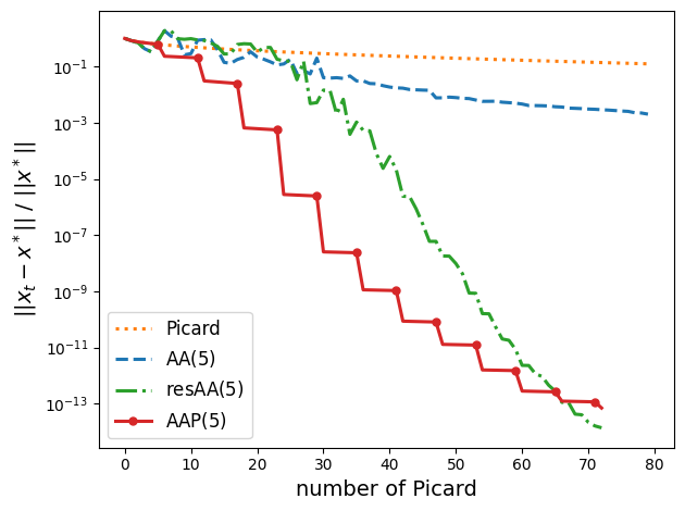
(a) w8a($m=5$)

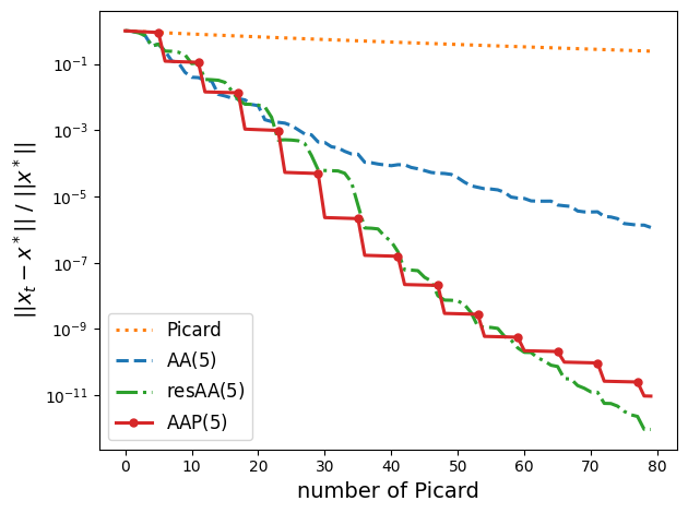
(b) covtype($m=5$)

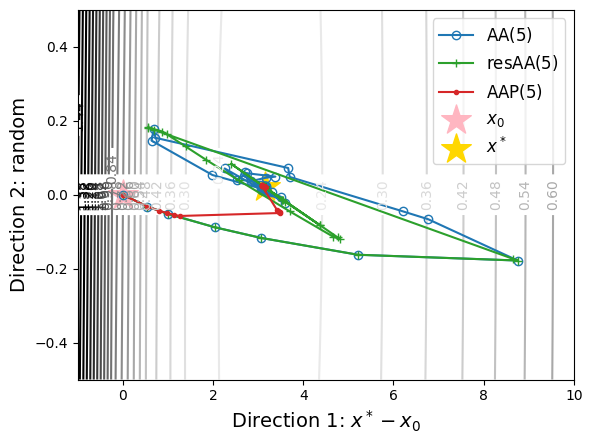
(c) w8a: optimization paths($m=5$)

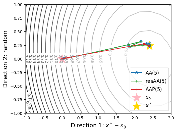
(d) covtype: optimization paths($m=5$)

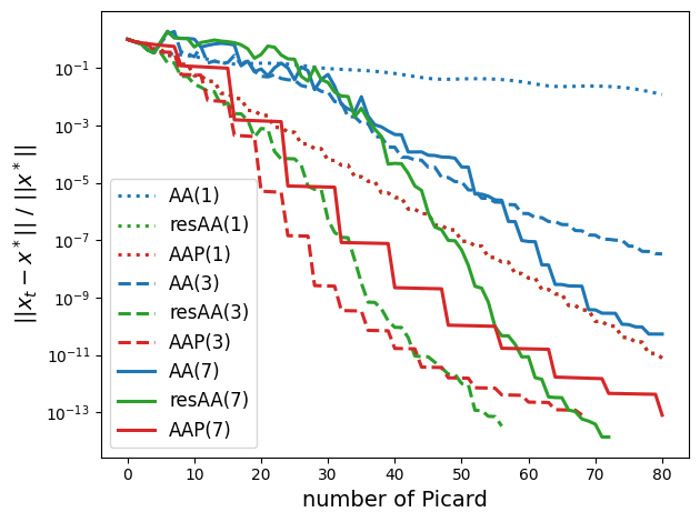
(e) w8a: varying $m$

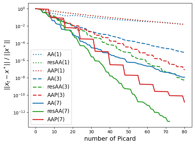
(f) covtype: varying $m$

Figure 1: Comparison of different algorithms applied to logistic regression with $\mu=0.01$ on both w8a and covtype datasets. First row: number of Picard iterations versus relative error. Second column: Landscape of the function $h$ and the optimization paths of different algorithms. The true domain dimension of $h$ is $300$ for the w8a dataset and $54$ for the covtype dataset. To visualize $h$, we show the level set of $h$ along two directions starting from the initial point $\boldsymbol{x}_{0}=0$: normalized $\boldsymbol{x}_{0}-\boldsymbol{x}^{*}$ and a random direction. The optimization paths are also projected onto these two directions, with each marker representing one Picard iteration. Due to the inefficiency of the history data points, the first $m$ iterations of AA($m$) are equivalent to those of resAA($m$), with their plots overlapping. Third row: effect of varying $m$ on different AA algorithms. It is noteworthy that when $m=1$, AAP($1$) is equivalent to resAA($1$), resulting in the vanishing plot of resAA($1$).

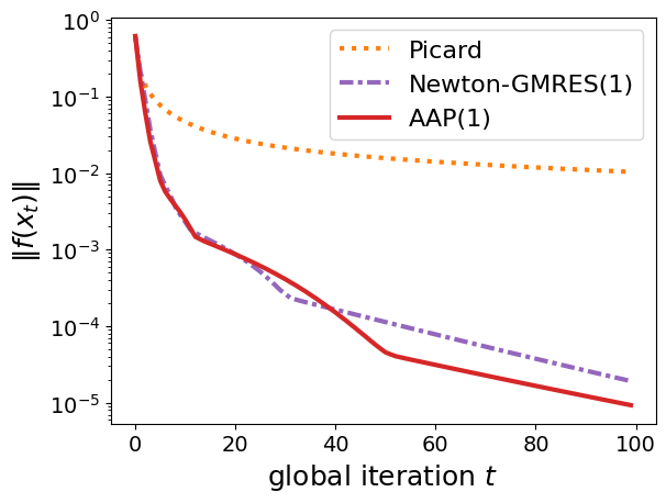
(a) $m=1$

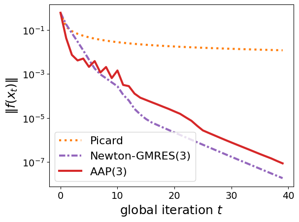
(b) $m=3$

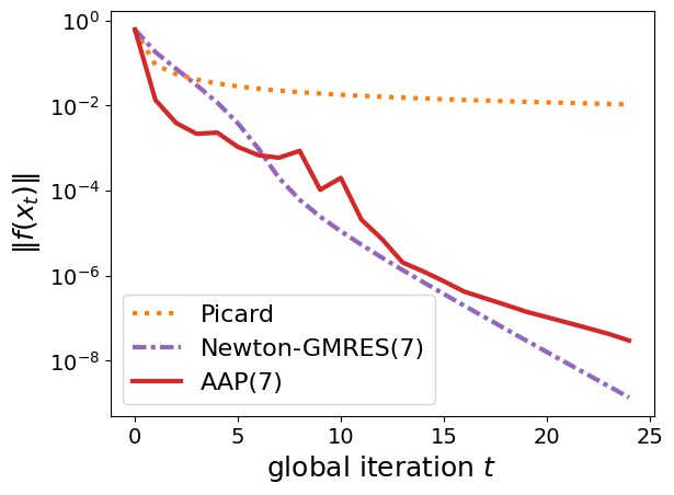
(c) $m=7$

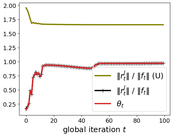
(d) $m=1$

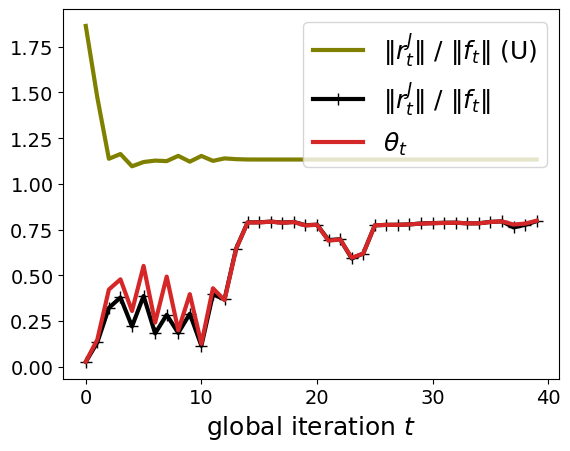
(e) $m=3$

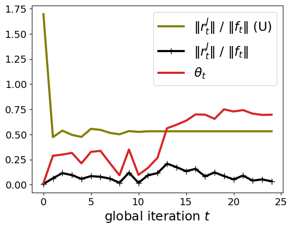
(f) $m=7$

Figure 2: Convergence of AAP on logistic regression with $\gamma=0.0001$ on the w8a dataset. The first row shows global iterations versus residual norm $\|f(\boldsymbol{x}_{t})\|$ for different algorithms, including Picard and Newton-GMRES as reference. In each global iteration, Picard performs $m+1$ steps to have a fair comparison with AAP. The second row presents global iterations versus optimization gain $\theta_{t}$. We also display the value of the Jacobian-GMRES gain $\|\boldsymbol{r}^{J}_{t}\|/\|\boldsymbol{f}_{t}\|$, as defined in (38). The Jacobian-GMRES gain $\|\boldsymbol{r}^{J}_{t}\|/\|\boldsymbol{f}_{t}\|$ (U) represents the theoretical upper bound of $\|\boldsymbol{r}^{J}_{t}\|/\|\boldsymbol{f}_{t}\|$ given in (41). Here the Jacobian is the Hessian of $h$, which is symmetric and positive definite.

6.2 Nonnegative matrix factorization

The second example is the Nonnegative Matrix Factorization (NMF) problem, which has been applied in fields such as text mining, image processing, and bioinformatics [11]. NMF decomposes a matrix $\boldsymbol{A}\in\mathbb{R}^{d_{1}\times d_{2}}$ into two nonnegative matrices $\boldsymbol{W}\in\mathbb{R}^{d_{1}\times r}$ and $\boldsymbol{H}\in\mathbb{R}^{r\times d_{2}}$, i.e., $\boldsymbol{A}\approx\boldsymbol{W}\boldsymbol{H}$ and $\boldsymbol{W}\geq 0,\boldsymbol{H}\geq 0$. The optimization problem associated with NMF can be formulated as

$$\min_{\boldsymbol{W},\boldsymbol{H}}\|\boldsymbol{A}-\boldsymbol{W}\boldsymbol{H}\|_{F}^{2}\quad\text{subject to}\quad\boldsymbol{W}\geq 0,\;\boldsymbol{H}\geq 0,$$

where $\|\cdot\|_{F}$ denotes the Frobenius norm. A widely used method to solve this problem is the alternating nonnegative least-squares (ANNLS) method: starting from $\boldsymbol{W}_{0}\geq 0$, one generates a sequence of $\left(\boldsymbol{W}_{t},\boldsymbol{H}_{t}\right)$ by alternately solving the standard nonnegatively constrained linear least-squares problems:

$$\boldsymbol{H}_{t}=\operatorname*{arg\,min}_{\boldsymbol{H}\geq 0}\|\boldsymbol{A}-\boldsymbol{W}_{t-1}\boldsymbol{H}\|_{F}\quad\text{and}\quad\boldsymbol{W}_{t}=\operatorname*{arg\,min}_{\boldsymbol{W}\geq 0}\|\boldsymbol{A}-\boldsymbol{W}\boldsymbol{H}_{t}\|_{F}.$$

Additionally, a normalization of $\boldsymbol{W}_{t}$ is applied at the beginning of each iteration. Following [37], we consider ANNLS to be a fixed-point iteration through the assignment $\left(\boldsymbol{W}_{t},\boldsymbol{H}_{t}\right)\rightarrow\left(\boldsymbol{W}_{t+1},\boldsymbol{H}_{t+1}\right)$. We perform the AA step on this problem by solving a constrained LS based on the vectorized variable, and we truncate $\left(\boldsymbol{W}_{t},\boldsymbol{H}_{t}\right)$ after the AA step to guarantee nonnegativity of the sequence.

We construct synthetic NMF problems by generating random matrices $\boldsymbol{W}\in\mathbb{R}^{300\times r}$ and $\boldsymbol{H}\in\mathbb{R}^{r\times 50}$, and then take $\boldsymbol{A}=\boldsymbol{W}\boldsymbol{H}\in\mathbb{R}^{300\times 50}$. Consequently, the minimum of the NMF objective function is zero. The initial point $\boldsymbol{W}_{0}$ is chosen randomly. Figure 3 presents the results of different algorithms with the same initialization. It is evident that all AA variants, including AAP, AA, and resAA, significantly improve convergence compared to ANNLS. Since performance of each algorithm can be influenced by different initializations, we also provide the median and interquartile range plots of 15 runs.

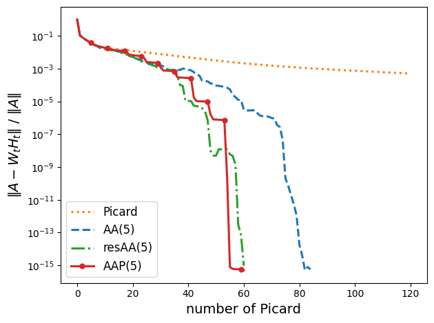
(a)

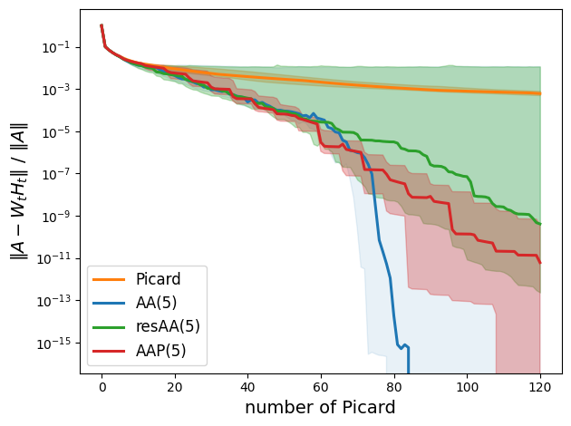
(b)

Figure 3: Comparison of different algorithms on NMF problems with $r=4$. All plot shows number of Picard iterations versus relative residual $\|\boldsymbol{A}-\boldsymbol{W}_{t}\boldsymbol{H}_{t}\|_{F}/\|\boldsymbol{A}\|_{F}$. (a): Different algorithms with the same initialization. (b): Median and interquartile range plots of 15 runs with random initializations.

7 Conclusion

This work focuses on the analysis of the Alternating Anderson Picard method, in which an Anderson acceleration step is periodically applied after a number of Picard iterations. We established the equivalence between AAP and multisecant-GMRES and explored the relation between AAP and Newton-GMRES, with particular emphasis on convergence analysis. We proved that the AAP residual converges locally at an improved rate when compared to Picard iteration. Numerically, this method has demonstrated efficiency and robustness in our evaluations and is comparable to the Newton-GMRES method without accessing the Jacobian. This underscores the potential of AAP as a practical alternative in scenarios where computational resources are limited or when explicit Jacobian computation is impractical.

Appendix A Uniform boundedness of $\mathrm{cond}(\boldsymbol{S}_{t})$

The uniform boundedness of $\mathrm{cond}(\boldsymbol{S}_{t})$ is important for the bound of $\boldsymbol{E}_{t}$ as shown in Theorem 4.3. Thus, in this section, we discuss $\mathrm{cond}(\boldsymbol{S}_{t})$ when the AAP residual $\boldsymbol{f}_{t}$ approaches $0$.

We have shown that $\boldsymbol{S}_{t}$ converges to $\boldsymbol{G}_{t}$ as $\|\boldsymbol{f}_{t}\|$ approaches zero. Consequently, $\mathrm{cond}(\boldsymbol{G}_{t})$ can serve as an estimator for $\mathrm{cond}(\boldsymbol{S}_{t})$ when $\|\boldsymbol{f}_{t}\|$ is sufficiently small. The matrix $\boldsymbol{G}_{t}$ is a Krylov matrix. The condition number and the least singular value of Krylov matrices are active research areas [5, 9, 4]. Generally speaking, $\boldsymbol{G}_{t}$ can be ill-conditioned even for a moderate number of columns [5].

In the following, we discuss $\mathrm{cond}(\boldsymbol{G}_{t})$ in a simple case where $g^{\prime}(\boldsymbol{x}_{t})$ is symmetric, allowing $\boldsymbol{G}_{t}$ to be decomposed into the product of a diagonal matrix and a Vandermonde matrix.

Lemma A.1.

Let $g^{\prime}(\boldsymbol{x}_{t})$be a symmetric matrix with eigendecomposition $g^{\prime}(\boldsymbol{x}_{t})=\boldsymbol{Q}^{T}\boldsymbol{\Lambda}\boldsymbol{Q}$, where $\boldsymbol{Q}$ is an orthogonal matrix and $\boldsymbol{\Lambda}=\operatorname{diag}(\lambda_{1},\ldots,\lambda_{d})$. Denote $\boldsymbol{Q}\frac{\boldsymbol{f}_{t}}{\|\boldsymbol{f}_{t}\|}=[a_{1},a_{2},\ldots,a_{d}]^{T}$. If $\min_{i}|a_{i}|>0$, then

(46) $$\mathrm{cond}(\boldsymbol{G}_{t})\leq\frac{\sqrt{m}}{\left(\min_{i}|a_{i}|\right)\,\sigma_{\min}\left(\boldsymbol{V}_{m}(\lambda_{1},\lambda_{2},\ldots,\lambda_{d})\right)},$$

where $\boldsymbol{V}_{m}(\lambda_{1},\ldots,\lambda_{d})$ is a $d\times m$ rectangular Vandermonde matrix.

Proof A.2.

Denote $\boldsymbol{K}=g^{\prime}(\boldsymbol{x}_{t})$. Since $\boldsymbol{K}=\boldsymbol{Q}^{T}\boldsymbol{\Lambda}\boldsymbol{Q}$, we have $\boldsymbol{K}^{(\ell)}=\boldsymbol{Q}^{T}\boldsymbol{\Lambda}^{(\ell)}\boldsymbol{Q}$. By the definition of $\boldsymbol{G}_{t}$, we have

$$\boldsymbol{Q}\boldsymbol{G}_{t} =\boldsymbol{Q}[\boldsymbol{f}_{t},\boldsymbol{K}^{(1)}\boldsymbol{f}_{t},\boldsymbol{K}^{(2)}\boldsymbol{f}_{t},\ldots,\boldsymbol{K}^{(m-1)}\boldsymbol{f}_{t}]$$

$$=[\boldsymbol{Q}\boldsymbol{f}_{t},\boldsymbol{Q}\boldsymbol{K}^{(1)}\boldsymbol{f}_{t},\boldsymbol{Q}\boldsymbol{K}^{(2)}\boldsymbol{f}_{t},\ldots,\boldsymbol{Q}\boldsymbol{K}^{(m-1)}\boldsymbol{f}_{t}]$$

$$=[\boldsymbol{Q}\boldsymbol{f}_{t},\boldsymbol{\Lambda}^{(1)}\boldsymbol{Q}\boldsymbol{f}_{t},\boldsymbol{\Lambda}^{(2)}\boldsymbol{Q}\boldsymbol{f}_{t},\ldots,\boldsymbol{\Lambda}^{(m-1)}\boldsymbol{Q}\boldsymbol{f}_{t}].$$

It follows from $\boldsymbol{Q}\frac{\boldsymbol{f}_{t}}{\|\boldsymbol{f}_{t}\|}=[a_{1},a_{2},\ldots,a_{d}]^{T}$ that

$$\frac{1}{\|\boldsymbol{f}_{t}\|}\boldsymbol{Q}\boldsymbol{G}_{t} =\begin{bmatrix}a_{1}&a_{1}\lambda_{1}&a_{1}\lambda_{1}^{2}&\cdots&a_{1}\lambda_{1}^{m-1}\\ a_{2}&a_{2}\lambda_{2}&a_{2}\lambda_{2}^{2}&\cdots&a_{2}\lambda_{2}^{m-1}\\ \vdots&\vdots&\vdots&\ddots&\vdots\\ a_{d}&a_{d}\lambda_{d}&a_{d}\lambda_{d}^{2}&\cdots&a_{d}\lambda_{d}^{m-1}\end{bmatrix}$$

$$=\operatorname{diag}(a_{1},a_{2},\ldots,a_{d})\boldsymbol{V}_{m}(\lambda_{1},\lambda_{2},\ldots,\lambda_{d}).$$

Denote $\boldsymbol{D}=\operatorname{diag}(a_{1},a_{2},\ldots,a_{d})$ and $\boldsymbol{V}=\boldsymbol{V}_{m}(\lambda_{1},\lambda_{2},\ldots,\lambda_{d})$. Since $\boldsymbol{Q}$ is an orthogonal matrix, we have

$$\textstyle\sigma_{\min}\left(\frac{1}{\|\boldsymbol{f}_{t}\|}\boldsymbol{G}_{t}\right)=\sigma_{\min}\left(\frac{1}{\|\boldsymbol{f}_{t}\|}\boldsymbol{Q}\boldsymbol{G}_{t}\right)=\sigma_{\min}\left(\boldsymbol{D}\boldsymbol{V}\right).$$

Assume $\sigma_{\min}(\boldsymbol{D}\boldsymbol{V})=\|\boldsymbol{D}\boldsymbol{V}\bar{\boldsymbol{x}}\|$ with $\|\bar{\boldsymbol{x}}\|$=1. Since $\sigma_{\min}(\boldsymbol{V})=\min_{\boldsymbol{x}\neq 0}\frac{\|\boldsymbol{V}\boldsymbol{x}\|}{\|\boldsymbol{x}\|}$,

$$\textstyle\sigma_{\min}(\boldsymbol{V})\leq\frac{\|\boldsymbol{V}\bar{\boldsymbol{x}}\|}{\|\bar{\boldsymbol{x}}\|}=\frac{\|\boldsymbol{D}^{-1}\boldsymbol{D}\boldsymbol{V}\bar{\boldsymbol{x}}\|}{\|\bar{\boldsymbol{x}}\|}\leq\|\boldsymbol{D}^{-1}\|\,\|\boldsymbol{D}\boldsymbol{V}\bar{\boldsymbol{x}}\|=\frac{1}{\min_{i}|a_{i}|}\|\boldsymbol{D}\boldsymbol{V}\bar{\boldsymbol{x}}\|.$$

Thus, $\sigma_{\min}\left(\frac{1}{\|\boldsymbol{f}_{t}\|}\boldsymbol{G}_{t}\right)\geq\left(\min_{i}|a_{i}|\right)\,\sigma_{\min}\left(\boldsymbol{V}\right)$. On the other hand, $\sigma_{\max}\left(\frac{1}{\|\boldsymbol{f}_{t}\|}\boldsymbol{G}_{t}\right)=\|\left(\frac{1}{\|\boldsymbol{f}_{t}\|}\boldsymbol{G}_{t}\right)\|\leq\|\left(\frac{1}{\|\boldsymbol{f}_{t}\|}\boldsymbol{G}_{t}\right)\|_{F}\leq\sqrt{m}$. Combining these with

$$\textstyle\mathrm{cond}(\boldsymbol{G}_{t})=\mathrm{cond}(\frac{1}{\|\boldsymbol{f}_{t}\|}\boldsymbol{G}_{t})=\sigma_{\max}\left(\frac{1}{\|\boldsymbol{f}_{t}\|}\boldsymbol{G}_{t}\right)/\sigma_{\min}\left(\frac{1}{\|\boldsymbol{f}_{t}\|}\boldsymbol{G}_{t}\right),$$

gives the result.

In Lemma A.1, the condition that $\min_{i}|a_{i}|>0$ is equivalent to the vector $\boldsymbol{f}_{t}$ not being parallel to any of the eigenvectors of the matrix $g^{\prime}(\boldsymbol{x}_{t})$. The least singular value of the Vandermonde matrix $\boldsymbol{V}_{m}(\lambda_{1},\ldots,\lambda_{d})$ depends on the distribution of its seeds $\lambda_{i}$ [4, 21, 9]. Theorem 6 of [9] shows that when the largest seed $|\lambda_{1}|<1$, the least singular value

$$\sigma_{\min}(\boldsymbol{V}_{m}(\lambda_{1},\ldots,\lambda_{d}))\leq\sigma_{\max}(\boldsymbol{V}_{m}(\lambda_{1},\ldots,\lambda_{d}))|\lambda_{1}|^{(m)},$$

which decays exponentially with respect to $m$. It indicates that a large $m$ may lead to a significant increase in $\mathrm{cond}(\boldsymbol{G}_{t})$, which in turn can cause a dramatic increase in $\|\boldsymbol{E}_{t}\|$. In addtion, since $\boldsymbol{S}_{t}\rightarrow\boldsymbol{G}_{t}$, and $\boldsymbol{Y}_{t}\rightarrow\boldsymbol{G}_{t}$, large $m$ may cause instability of the least square problem in the AA step. However, when $\boldsymbol{f}_{t}$ is small, machine round-off errors will also affect the numerical value of $\mathrm{cond}(\boldsymbol{S}_{t})$ and $\mathrm{cond}(\boldsymbol{Y}_{t})$.

References

• [1] H.-B. An and Z.-Z. Bai, A globally convergent newton-gmres method for large sparse systems of nonlinear equations, Applied Numerical Mathematics, 57 (2007), pp. 235–252.
• [2] D. G. Anderson, Iterative procedures for nonlinear integral equations, Journal of the ACM (JACM), 12 (1965), pp. 547–560.
• [3] A. S. Banerjee, P. Suryanarayana, and J. E. Pask, Periodic Pulay method for robust and efficient convergence acceleration of self-consistent field iterations, Chemical Physics Letters, 647 (2016), pp. 31–35.
• [4] F. S. Bazán, Conditioning of rectangular Vandermonde matrices with nodes in the unit disk, SIAM Journal on Matrix Analysis and Applications, 21 (2000), pp. 679–693.
• [5] B. Beckermann, The condition number of real Vandermonde, Krylov and positive definite Hankel matrices, Numerische Mathematik, 85 (2000), pp. 553–577.
• [6] C.-C. Chang and C.-J. Lin, Libsvm: a library for support vector machines, ACM Transactions on Intelligent Systems and Technology (TIST), 2 (2011), pp. 1–27.
• [7] X. Chen and C. T. Kelley, Convergence of the EDIIS algorithm for nonlinear equations, SIAM Journal on Scientific Computing, 41 (2019), pp. A365–A379.
• [8] R. Choquet and J. Erhel, Some convergence results for the Newton-GMRES algorithm, PhD thesis, INRIA, 1993.
• [9] A. Dax, The numerical rank of Krylov matrices, Linear Algebra and Its Applications, 528 (2017), pp. 185–205.
• [10] R. S. Dembo, S. C. Eisenstat, and T. Steihaug, Inexact newton methods, SIAM Journal on Numerical analysis, 19 (1982), pp. 400–408.
• [11] L. Eldén, Matrix methods in data mining and pattern recognition, SIAM, 2019.
• [12] C. Evans, S. Pollock, L. G. Rebholz, and M. Xiao, A proof that Anderson acceleration improves the convergence rate in linearly converging fixed-point methods (but not in those converging quadratically), SIAM Journal on Numerical Analysis, 58 (2020), pp. 788–810.
• [13] H.-r. Fang and Y. Saad, Two classes of multisecant methods for nonlinear acceleration, Numerical linear algebra with applications, 16 (2009), pp. 197–221.
• [14] X. Feng, Anderson Acceleration and Dynamic Optimal Transport in Optimization: Theoretical Analysis, Algorithms, and Applications in Machine Learning, University of California, Davis, 2024.
• [15] M. Geist and B. Scherrer, Anderson acceleration for reinforcement learning, arXiv preprint arXiv:1809.09501, (2018).
• [16] G. H. Golub and C. F. Van Loan, Matrix computations, JHU press, 2013.
• [17] A. Greenbaum and Z. Strakos, Matrices that generate the same Krylov residual spaces, Springer, 1994.
• [18] A. Han, B. Mishra, P. Jawanpuria, and J. Gao, Riemannian accelerated gradient methods via extrapolation, in International Conference on Artificial Intelligence and Statistics, PMLR, 2023, pp. 1554–1585.
• [19] C. T. Kelley, Numerical methods for nonlinear equations, Acta Numerica, 27 (2018), pp. 207–287.
• [20] D. A. Knoll and D. E. Keyes, Jacobian-free Newton–Krylov methods: a survey of approaches and applications, Journal of Computational Physics, 193 (2004), pp. 357–397.
• [21] S. Kunis and D. Nagel, On the condition number of Vandermonde matrices with pairs of nearly-colliding nodes, Numerical Algorithms, 87 (2021), pp. 473–496.
• [22] P. A. Lott, H. F. Walker, C. S. Woodward, and U. M. Yang, An accelerated Picard method for nonlinear systems related to variably saturated flow, Advances in Water Resources, 38 (2012), pp. 92–101.
• [23] M. Lupo Pasini, Convergence analysis of Anderson-type acceleration of Richardson’s iteration, Numerical Linear Algebra with Applications, 26 (2019), p. e2241.
• [24] J. Nocedal and S. J. Wright, Numerical optimization, Springer, 1999.
• [25] W. Ouyang, Y. Liu, and A. Milzarek, Descent properties of an Anderson accelerated gradient method with restarting, SIAM Journal on Optimization, 34 (2024), pp. 336–365.
• [26] W. Ouyang, Y. Peng, Y. Yao, J. Zhang, and B. Deng, Anderson acceleration for nonconvex ADMM based on Douglas-Rachford splitting, in Computer Graphics Forum, vol. 39, Wiley Online Library, 2020, pp. 221–239.
• [27] Y. Peng, B. Deng, J. Zhang, F. Geng, W. Qin, and L. Liu, Anderson acceleration for geometry optimization and physics simulation, ACM Transactions on Graphics, 37 (2018), p. Article 42.
• [28] S. Pollock, L. Rebholz, and M. Xiao, Anderson-accelerated convergence of Picard iterations for incompressible Navier-Stokes equations, SIAM Journal on Numerical Analysis, 57 (2019), pp. 615–637.
• [29] S. Pollock and L. G. Rebholz, Anderson acceleration for contractive and noncontractive operators, IMA Journal of Numerical Analysis, 41 (2021), pp. 2841–2872.
• [30] S. Pollock and L. G. Rebholz, Filtering for Anderson acceleration, SIAM Journal on Scientific Computing, 45 (2023), pp. A1571–A1590.
• [31] P. P. Pratapa, P. Suryanarayana, and J. E. Pask, Anderson acceleration of the Jacobi iterative method: An efficient alternative to Krylov methods for large, sparse linear systems, Journal of Computational Physics, 306 (2016), pp. 43–54.
• [32] J. A. Sifuentes, M. Embree, and R. B. Morgan, GMRES convergence for perturbed coefficient matrices, with application to approximate deflation preconditioning, SIAM Journal on Matrix Analysis and Applications, 34 (2013), pp. 1066–1088.
• [33] H. D. Sterck and Y. He, On the asymptotic linear convergence speed of Anderson acceleration, Nesterov acceleration, and nonlinear GMRES, SIAM Journal on Scientific Computing, 43 (2021), pp. S21–S46.
• [34] G. W. Stewart, On the perturbation of pseudo-inverses, projections and linear least squares problems, SIAM review, 19 (1977), pp. 634–662.
• [35] P. Suryanarayana, P. P. Pratapa, and J. E. Pask, Alternating Anderson–Richardson method: An efficient alternative to preconditioned Krylov methods for large, sparse linear systems, Computer Physics Communications, 234 (2019), pp. 278–285.
• [36] A. Toth and C. T. Kelley, Convergence analysis for Anderson acceleration, SIAM Journal on Numerical Analysis, 53 (2015), pp. 805–819.
• [37] H. F. Walker and P. Ni, Anderson acceleration for fixed-point iterations, SIAM Journal on Numerical Analysis, 49 (2011), pp. 1715–1735.
• [38] D. Wang, Y. He, and H. De Sterck, On the asymptotic linear convergence speed of Anderson acceleration applied to ADMM, Journal of Scientific Computing, 88 (2021), p. 38.
• [39] J. Zhang, B. O’Donoghue, and S. Boyd, Globally convergent type-I Anderson acceleration for nonsmooth fixed-point iterations, SIAM Journal on Optimization, 30 (2020), pp. 3170–3197.