Nucleation of de Sitter from the anti de Sitter spacetime in scalar field models

Abstract

We show that, in the framework of Einstein-scalar gravity, the de Sitter (dS) spacetime can be nucleated out of the anti de Sitter (AdS) one. This is done by using a scalar lump solution, which has an $\text{AdS}_{4}$ spacetime in the core, allows for $\text{dS}_{4}$ vacua and was found to be plagued by tachyonic instabilities. Using the Euclidean action formalism, we compute and compare the probability amplitudes and the free energies of the lump and the $\text{dS}_{4}$ vacua. Our results show that the former is generally less favored than the latter, with the most preferred state being a $\text{dS}_{4}$ vacuum. The lump, thus, describes a metastable state which eventually decays into the true $\text{dS}_{4}$ vacuum. This nucleation mechanism of dS spacetime may provide insights into the short-distance behavior of gravity, in particular for the characterization of string-theory vacua, cosmological inflation and the black-hole singularity problem.

I Introduction

Observational evidence [1, 2, 3, 4, 5, 6] has robustly established that our universe is undergoing a phase of exponential expansion. This phenomenon, also believed to have occurred shortly after the big bang during the inflationary phase [7, 8, 9, 10, 11], is well-described by the de Sitter (dS) solution within General Relativity (GR). However, a GR description of the primordial universe is expected to be unreliable and a theory of quantum gravity is required.

String theory holds promise to be such a candidate, offering valuable tools to address numerous questions in quantum gravity. However, stable (or even metastable) dS vacua without tachyonic excitations are difficult to accommodate within such a theory, as suggested by several no-go theorems. This has also led to the conjecture that dS vacua may actually not exist in string theory, relegating them in the so-called swampland (see Refs. [12, 13, 14, 15, 16, 17, 18, 19, 20, 21] for particular realizations, which however raised several concerns; for discussions on the latter, other related aspects and no-go theorems, see, e.g., Refs. [22, 23, 24, 25, 26, 27, 28, 29, 30, 31, 32, 33, 34, 35, 36, 37]). This challenge seems common to general quantum gravity frameworks [38, 39, 40, 41]. The main difficulty is that the typical four-dimensional potential $V$ of a scalar theory arising from compactifications of higher dimensional string theory/M theory does not admit any stationary point where $V>0$. In contrast, negative-energy vacua, which are compatible with an anti de Sitter (AdS) spacetime, seem to fit better, aligning with the usual zero-point energy in quantum field theory.

In the present letter, we revisit the issue of the emergence of a dS spacetime by working in the framework of four-dimensional Einstein-scalar gravity. This approach is inspired and motivated by the natural emergence of scalar fields in string theory compactifications, their usefulness in modelling inflation, and their role in constructing regular (singularity-free) compact object solutions that interpolate between AdS and dS spacetimes in different regimes [42, 43]. Furthermore, recent studies in two-dimensional dilatonic theories have shown the emergence of dS spacetime from AdS fluctuations [44, 45]. The nucleation of a dS spacetime is also relevant in the context of regular black holes, which often exhibit cores with a dS geometry [46, 47, 48, 49]. Finally, recent calculations in the Functional Renormalization Group framework show the emergence of such a dS core from an AdS one [50].

Here we consider the regular lump solution of Ref. [43], which interpolates between an $\text{AdS}_{4}$ spacetime in the core and a $\text{dS}_{2}\times\text{S}^{2}$ topology at infinity. Notably, the scalar potential generating such solution also features stationary points where the geometry is $\text{dS}_{4}$, with one being an absolute stable minimum. We show that the lump instability, initially investigated in Ref. [43] and explored further here, makes this solution a metastable state which eventually decays into the true, stable $\text{dS}_{4}$ vacuum.

II Existence of (A)dS interpolating solutions in Einstein-Scalar gravity

We consider Einstein’s gravity minimally coupled to a real scalar field $\phi$

$$\mathcal{S}=\int\text{d}^{4}x\,\sqrt{-g}\left(\mathscr{R}-\frac{1}{2}g^{\mu\nu}\partial_{\mu}\phi\partial_{\nu}\phi-V(\phi)\right)\,,$$ (1)

where $\mathscr{R}$ is the Ricci scalar, while $V(\phi)$ is the self-interaction potential. The field equations read

$$\begin{split}G_{\mu\nu}&=\frac{1}{2}T_{\mu\nu}\,,\qquad\Box\phi=\frac{\text{d}V}{\text{d}\phi}\,,\\ T_{\mu\nu}&=-g_{\mu\nu}\left(\frac{1}{2}\partial_{\alpha}\phi\partial^{\alpha}\phi+V\right)+\partial_{\mu}\phi\partial_{\nu}\phi\,.\end{split}$$ (2)

In the following, we will deal with spherically-symmetric, static solutions of the form

$$\begin{split}\text{d}s^{2}&=-U(r)\text{d}t^{2}+U(r)^{-1}\text{d}r^{2}+R(r)^{2}\text{d}\Omega^{2}\,,\\ \phi&=\phi(r)\,.\end{split}$$ (3)

The field equations (2) then read

$$\phi^{\prime\prime}=-\left(2\frac{R^{\prime}}{R}+\frac{U^{\prime}}{U}\right)\phi^{\prime}+\frac{1}{U}\frac{\text{d}V}{\text{d}\phi}\,;$$ (4a)

$$U^{\prime\prime}=-2\frac{R^{\prime}}{R}U^{\prime}-V\,;$$ (4b)

$$\frac{R^{\prime\prime}}{R}=-\frac{1}{4}\phi^{\prime 2}\,;$$ (4c)

$$UR^{\prime 2}-1+URR^{\prime\prime}-\frac{U^{\prime\prime}}{2}R^{2}=0\,.$$ (4d)

Constant scalar-field configurations correspond to standard GR solutions (vacua)

$$R(r)=r\,,\qquad U_{\text{GR}}=1-\frac{V(\phi_{0})}{6}r^{2}\,,\qquad\phi(r)=\phi_{0}\,.$$ (5)

Equation 5 is a solution of the equations (4) if and only if $\phi_{0}$ corresponds to the position of an extremum of the potential $V(\phi)$. Depending on the sign of $V(\phi_{0})$, Eq. 5 describes Minkowski, dS or AdS vacua for $V(\phi_{0})=0$, $V(\phi_{0})>0$ or $V(\phi_{0})<0$, respectively. In the latter two cases, the (A)dS length is determined through $|V(\phi_{0})|/6=L^{-2}$.

Apart from the standard GR ones, the theory allows also for vacua with $\text{dS}_{2}\times\text{S}^{2}$ topology, always located at extrema of the potential $V(\phi)$:

$$R=\sqrt{\frac{2}{V(\phi_{0})}}\,,\quad U_{\text{GR}}=1-\frac{V(\phi_{0})}{2}r^{2}\,,\quad\phi(r)=\phi_{0}\,.$$ (6)

Equations 5 and 6 are not the most general solutions of the theory (1) endowed with a trivial scalar field. In Eq. 5 we may include the Schwarzschild term $c_{1}/r$. Moreover, depending on the shape of the potential $V(\phi)$, we may have also solutions with a nontrivial $\phi(r)$ profile. In this paper, we are interested in solutions which are regular in the near $r=0$ region (the core) and have regular asymptotics at $r\to\infty$. As first observed in Ref. [42] and analyzed in details in Ref. [43], setting $c_{1}=0$ is necessary to construct smooth and regular solutions in the core. One might also consider subleading terms with respect to $r^{2}$ in the metric function, such as $U=1-\alpha+\beta r+\lambda r^{2}+\mathcal{O}(r^{3})$. However, the $\alpha$-term produces a curvature singularity of order $\mathcal{O}(r^{-2})$, while the $\beta$-one yields a singularity of order $\mathcal{O}(r^{-1})$. Therefore, Eq. 5 represents the most general solution in the core without curvature singularities.

One important point when dealing with regular solutions of Eq. 4 is the existence of configurations interpolating between different vacua, as described by (5) and (6), in the regions $r=0$ and $r\to\infty$. These configurations can appear both as isolated solutions, corresponding to extrema of the potential, or as approximate ones in the $r=0$ and $r\to\infty$ regions of an interpolating solution. In the latter case, Eqs. 5 and 6 provide the leading terms of the series expansion for this configuration. However, the existence of interpolating solutions with the regular behavior (5) in the core is not generally granted. We will explore this issue in the next section.

II.1 Nonexistence of interpolating solutions with pure (A)dS vacua in the core

Several no-go theorems in Einstein-scalar gravity [51, 52, 53, 43] show that solutions of Eq. 2 cannot interpolate between a dS spacetime at $r\sim 0$ and either a Minkowski or AdS spacetime at $r\to\infty$. However, this theorems does not preclude the possibility of interpolation between two dS spacetimes, nor does it exclude the presence of AdS or Minkowski cores.

In the following, we extend these results by proving that solutions interpolating between the Minkowski or (A)dS exact vacua (5) in the core and any arbitrary nontrivial solution outside cannot exist within the framework of the theory (1). The only allowed vacua are isolated GR solutions with a trivial scalar field profile. To do so, we start by assuming that it exists a quadratic extremum for $\phi=\phi_{0}$ of the potential at $r\sim 0$ and work out the solution perturbatively using the field equations (4).

The scalar potential we start from is of the form

$$V(\phi)=\Lambda+V_{1}\phi+V_{2}\phi^{2}+\mathcal{O}[(\phi-\phi_{0})^{3}]\,,$$ (7)

where $\Lambda$, $V_{1}$ and $V_{2}$ are constants. Equation 7 is quite general, as the linear term can always be introduced through a translation of $\phi$. While this translation results in a shift in the position of the extremum, it does not affect our overall conclusions. $V_{1,2}$ determine the value of $\phi_{0}$

$$\phi_{0}=-\frac{V_{1}}{2V_{2}}\,.$$ (8)

If we expand the metric and scalar-field solutions in power series around $r\sim 0$, Eq. 4 constrain the expansions to be (see also Ref. [54])

$$\phi(r)=\phi_{0}+\phi_{2}r^{2}+\phi_{4}r^{4}+\mathcal{O}(r^{6})\,;$$ (9a)

$$U(r)=1+U_{2}r^{2}+U_{4}r^{4}+\mathcal{O}(r^{6})\,;$$ (9b)

$$R(r)=r+R_{5}r^{5}+\mathcal{O}(r^{7})\,,$$ (9c)

where $\phi_{2}$, $\phi_{4}$, $U_{2}$, $U_{4}$, $R_{5}$ are constants. $U_{2}=0$, $U_{2}>0$ or $U_{2}<0$ imply a Minkowski, AdS or dS behavior near $r\sim 0$, respectively.

Plugging Eq. 9 into Eq. 4c and expanding near $r\sim 0$ yields

$$\left(80R_{5}+4\phi_{2}^{2}\right)r^{2}+\mathcal{O}(r^{4})=0\,.$$ (10)

For this to be satisfied at the order considered, we must require $\phi_{2}=2\sqrt{5}\sqrt{-R_{5}}$ and $R_{5}\leq 0$.

From Eq. 4d, one gets

$$\left(-5U_{4}+30R_{5}\right)r^{4}+\mathcal{O}(r^{5})=0\,,$$ (11)

from which one obtains $U_{4}=6R_{5}$ at leading order.

From Eq. 4b, one obtains

$$\left(6U_{2}+\Lambda-V_{2}\phi_{0}^{2}\right)+120R_{5}r^{2}+\mathcal{O}(r^{4})=0\,.$$ (12)

This fixes, at the zeroth order, $U_{2}=\left(-\Lambda+V_{2}\phi_{0}^{2}\right)/6$, while, at the $\mathcal{O}(r^{2})$ order, $R_{5}=0$. Therefore, the asymptotic solution (9) becomes

$$\phi=\phi_{0}+\mathcal{O}(r^{4})$$ (13a)

$$U(r)=1+\frac{-\Lambda+V_{2}\phi_{0}^{2}}{6}r^{2}+\mathcal{O}(r^{6})\,;$$ (13b)

$$R(r)=r+\mathcal{O}(r^{7})\,.$$ (13c)

Using a similar procedure, it is straightforward to demonstrate that even higher-order terms are constrained to vanish by the field equations.

We thus conclude that solutions interpolating between Minkowski or (A)dS quadratic vacua in the core and other nontrivial solutions outside are not permitted. Only isolated GR vacua with a trivial scalar field are allowed.

III Approximate solutions with a linear potential

The results of the previous section constrain the shape of the scalar-field potential in the solution core, as no potential extrema are allowed at $r=0$. However, they do not exclude the possibility of an approximate Minkowski/(A)dS solution in the core. For instance, solutions exhibiting AdS behavior in the core are already known [42, 43]. Consistently with our findings, in all known cases, the AdS geometry in the core is not sourced by a constant scalar field and does not correspond to any local extremum of $V$. Instead, it is sourced by a nontrivial $\phi(r)$ and is generated by a potential which typically behaves linearly in $\phi$. An important feature of these configurations is that they must necessarily be approximate solutions of the field equations.

Let us now investigate approximate solutions with a linear potential in the core. By setting $V_{2}=0$ in Eq. 7, we focus on the expansion at $r\sim 0$ given by Eq. 9. Substituting it into the field equations (4) yields

$$\phi(r) =\phi_{0}+2\sqrt{-5R_{5}}\,r^{2}$$

$$+\frac{\sqrt{-5R_{5}}\Lambda-60R_{5}\phi_{0}}{6}r^{4}+\mathcal{O}(r^{6})\,;$$ (14a)

$$U(r) =1-\frac{\Lambda+V_{1}\phi_{0}}{6}r^{2}+6R_{5}r^{4}+\mathcal{O}(r^{6})\,;$$ (14b)

$$R(r) =r+R_{5}r^{5}+\mathcal{O}(r^{7})\,,$$ (14c)

together with the requirement $R_{5}\leq 0$. At leading order (when terms proportional to $R_{5}$ or higher are neglected), the spacetime in the core is given by the vacuum solution (5). This results in Minkowski, dS or AdS solutions for $\Lambda=-V_{1}\phi_{0}$, $\Lambda>-V_{1}\phi_{0}$ or $\Lambda<-V_{1}\phi_{0}$, respectively. Unlike the case discussed in the previous section, these approximate solutions do not correspond to extrema of the potential. Therefore, their existence is allowed in global solutions that interpolate between Minkowski or (A)dS geometries in the core and nontrivial configurations at spatial infinity, compatibly with the no-go theorem established in [43].

We conclude this section by highlighting the relevance of linear potentials from various perspectives. Firstly, they arise in axion inflationary scenarios within string theory, specifically in axion monodromy inflation. The latter arises from the compactification of a D$5$-brane in type IIB string theory. In four dimensions and for large values of the axion, this setup produces a linear scalar potential [55, 56, 57]. Additionally, linear inflation also naturally emerges as a solution in Coleman-Weinberg inflation [58], provided the inflaton has a nonminimal coupling to gravity and the Planck scale is dynamically generated [59]. The most intriguing application of Einstein-scalar gravity with an approximate linear potential, which we will focus on in the remainder of this paper, is related to their use in describing the cores of compact objects. The cores of several nonsingular scalar solutions, such as the Sine-Gordon solitonic configuration analyzed in Ref. [42], or the regular lump solution found in Ref. [43], are described by an AdS spacetime sourced by an approximate linear potential. These solutions typically exhibit dynamical instabilities, most commonly tachyonic ones, although the instability timescale could also be quite long. Consequently, these solutions can be considered metastable states which eventually tunnel to a stable vacuum of the theory. The primary application we envision is a tunnelling process between an AdS and a dS spacetime, mediated by an unstable solution of the kind described above. This nucleation of dS out of AdS is potentially very interesting for several applications, including characterization of string theory vacua, inflation and the black-hole singularity problem.

In the following, we will consider the lump solution of Ref. [43] as a specific model to describe this nucleation. However, we expect this to be just a particular case of a quite general class of Einstein-scalar gravity models.

IV Scalar lump solution

The regular lump spacetime of Ref. [43] is of the form (3),with

$$R(r) =\frac{r}{\left[1+\left(\frac{r}{\ell}\right)^{4}\right]^{1/4}}\,;$$ (15a)

$$U(r) =\frac{c_{2}r^{2}\ell^{4}-r^{4}+\ell^{4}}{\ell^{2}\sqrt{r^{4}+\ell^{4}}};$$ (15b)

$$\phi(r) =\sqrt{5}\,\tan^{-1}\left(\frac{\ell^{2}}{r^{2}}\right)\,;$$ (15c)

$$V(r) =\frac{2\left(5c_{2}r^{4}\ell^{8}-3c_{2}\ell^{12}+r^{10}+15r^{2}\ell^{8}\right)}{\ell^{2}\left(r^{4}+\ell^{4}\right)^{5/2}}\,,$$ (15d)

where $\ell$ is an arbitrary length-scale characterizing the potential $V$, and $c_{2}$ an integration constant that must be positive to ensure the metric signature does not change anywhere (see Ref. [43] for details). By inverting Eq. 15c we can also express the potential as a function of $\phi$ (see Fig. 1 for a qualitative plot)

$$\begin{split}V(\phi)=&\frac{2}{\ell^{2}}\biggl{\{}c_{2}\ell^{2}\left[5\cot^{2}\left(\frac{\phi}{\sqrt{5}}\right)-3\right]\\ &+\cot\left(\frac{\phi}{\sqrt{5}}\right)\left[\cot^{4}\left(\frac{\phi}{\sqrt{5}}\right)+15\right]\biggr{\}}\times\\ &\times\sin^{5}\left(\frac{\phi}{\sqrt{5}}\right)\,.\end{split}$$ (16)

Near $r\sim 0$, $R(r)\sim r$, while at infinity, $R(r)\sim\ell=\text{constant}$. $U$, instead, exhibits a dS asymptotics at infinity, with a dS length $\ell$, while near $r\sim 0$, the spacetime is AdS, with $c_{2}$ giving the inverse of the square of the AdS length. Expanding the solution (15) near $r=0$ and the potential (16) near $\phi=0$, one easily finds that the lump behaves in the core exactly as the approximate AdS solution (14) with the linear potential described in the previous section. Therefore, the lump spacetime interpolates between $\text{AdS}_{4}$ spacetime at $r\sim 0$ and a Nariai spacetime $\text{dS}_{2}\times\text{S}^{2}$ at $r\to\infty$. The scalar field, instead, is a limited function between $\phi(r=0)=\sqrt{5}\pi/2$ and $\phi(r\to\infty)=0$.

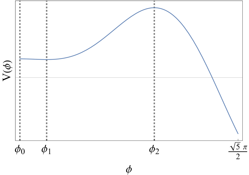
Figure 1: Qualitative behavior of the scalar lump potential as a function of $\phi$. The right side of the horizontal axis corresponds to the $r\to 0$ region, where $\phi(0)=\sqrt{5}\pi/2$, while the left side corresponds to the $r\to\infty$ region. The vertical dashed lines indicate the positions of the extrema, corresponding to $\text{dS}_{4}$ vacua.

IV.0.1 de Sitter vacua

As illustrated in Fig. 1, the potential (16), apart from the exact lump solution (15), allows for exact GR vacua. In the interval $\phi\in[0,\sqrt{5}\,\pi/2]$, they correspond to the three extrema $\phi_{0}=0$, $\phi_{1}$ and $\phi_{2}$ (whose values depend on $c_{2}$). Depending on the chosen spacetime topology, they correspond either to pure $\text{dS}_{4}$ (see Eq. 5) or $\text{dS}_{2}\times\text{S}^{2}$ (see LABEL:{ds2solutions}) vacua. Notice that the topology of the $\phi_{0}$ vacuum is fixed to be $\text{dS}_{2}\times\text{S}^{2}$ if it is not isolated, but generated in the $r\to\infty$ region by the interpolating lump solution (15). Conversely, there is no natural topology choice for $\phi_{1,2}$-vacua.

Since the value of $c_{2}$ does not alter the relevant physical results, we will, for simplicity, set $c_{2}=\ell^{-2}$. The position of the extrema and the corresponding values of the potential computed at these points are as follows

$$\phi_{0} =0\,, V(\phi_{0})=\frac{2}{\ell^{2}}\,;$$

$$\phi_{1} \simeq 0.430664\,, V(\phi_{1})\simeq\frac{1.92736}{\ell^{2}}\,;$$

$$\phi_{2} \simeq 2.16417\,, V(\phi_{2})\simeq\frac{7.4697}{\ell^{2}}\,.$$ (17)

Their dS horizons are given by

$$r^{(i)}_{\text{H, dS}}=\sqrt{\frac{6}{V(\phi_{i})}}\,,\quad i=0,1,2\,,$$ (18)

with the associated temperatures

$$T^{(i)}_{\text{H, dS}}=-\frac{U^{\prime}_{\text{dS}}\left(r^{(i)}_{\text{H, dS}}\right)}{4\pi}=\frac{\sqrt{V(\phi_{i})}}{2\sqrt{6}\,\pi}\,.$$ (19)

IV.0.2 Cosmological horizon and temperature of the lump

Owing to the dS asymptotic behavior, the metric function (15b) has a cosmological horizon located at $U(r_{\text{H}})=0$,

$$r_{\text{H}}=\frac{\ell}{\sqrt{2}}\sqrt{1+\sqrt{5}}\,.$$ (20)

The corresponding horizon temperature is given by

$$T_{\text{H}}=\frac{\sqrt[4]{5}}{2\pi\ell}\,.$$ (21)

IV.1 Nucleation of $\text{dS}_{4}$ from $\text{AdS}_{4}$ in the Euclidean action formalism

It has been shown in Ref. [43] that the scalar lump (15) is plagued by a tachyonic instability. Thus, it can be regarded as a metastable state, representing a decay mode of the $\text{AdS}_{4}$ core-vacuum (14) in the linear potential model. The presence of the $\text{dS}_{4}$/$\text{dS}_{2}\times\text{S}^{2}$ vacua in the model suggests that the scalar lump will decay into one of the latter. The most favored vacuum can be determined either thermodynamically, by computing the free energies, or by determining the relative probability of the different configurations. Both methods can be implemented using the Euclidean action formalism.

In the following, therefore, we exploit the semiclassical correspondence between the Euclidean action and the partition function in the canonical ensemble [60]

$$\mathcal{S}_{\text{E}}=-\ln\mathcal{Z}=\beta F\,.$$ (22)

$\beta$ is the inverse temperature of the ensemble, while $F$ is the free energy. $\mathcal{S}_{\text{E}}$ has to be computed on shell, for a given classical configuration representing the Gibbons saddle of the path integral, corresponding to a classical Euclidean instanton. $\mathcal{S}_{\text{E}}$ also allows to evaluate the non-normalized probability amplitude

$$\Gamma=\text{e}^{-\mathcal{S}_{\text{E}}}\,,$$ (23)

of realizing the configuration.

The Euclidean manifold of the lump is compact, given its dS asymptotics. Just as in pure dS spacetime [60], thus, we do not need to support the bulk action with boundary terms. One has, thus,

$$\mathcal{S}_{\text{E}}=-\int\text{d}^{4}x\,\sqrt{g_{\text{E}}}\left(\mathscr{R}-\frac{1}{2}g^{\mu\nu}\partial_{\mu}\phi\partial_{\nu}\phi-V\right)\,.$$ (24)

Exploiting Eq. 2, on shell, we have $\mathscr{R}=\partial_{\alpha}\phi\partial^{\alpha}\phi/2+2V$. Equation 24, thus, yields

$$\begin{split}\mathcal{S}_{\text{E}}&=-\int\text{d}^{4}x\,\sqrt{g_{\text{E}}}\,V\\ &=-4\pi\beta_{\text{Lump}}\int_{0}^{r_{\text{H}}}\text{d}r\,R^{2}(r)\,V(r)\,,\end{split}$$ (25)

where $\beta_{\text{Lump}}$ is the inverse of the temperature (21). Using Eqs. 15a, 15d, 20 and 21, we obtain

$$\mathcal{S}_{\text{E}}=-\frac{8\sqrt{2}\left(\sqrt{5}+5\right)^{3/2}\pi^{2}\ell^{2}}{5\left(\sqrt{5}+1\right)}\simeq-134.329\,\ell^{2}\,.$$ (26)

We now compare it with the Euclidean action of the $\text{dS}_{4}$ vacua, which reads [60]

$$\mathcal{S}_{\text{dS}}=-16\pi^{2}L^{2}=-\frac{96\pi^{2}}{V(\phi_{i})}\,,$$ (27)

where, in the second step, we have exploited the relation $V(\phi_{i})/6=L^{-2}$ (see below Eq. 5). For the vacua (17), one has

$$\phi_{0} =0\,, \mathcal{S}_{\text{dS, 0}}=-48\pi^{2}\,\ell^{2}\simeq-473.741\,\ell^{2}\,;$$

$$\phi_{1} \simeq 0.430664\,, \mathcal{S}_{\text{dS, 1}}\simeq-491.596\,\ell^{2}\,;$$

$$\phi_{2} \simeq 2.16417\,, \mathcal{S}_{\text{dS, 2}}\simeq-126.843\,\ell^{2}\,.$$ (28)

From these results, it is evident that the probability amplitude to generate the lump is lower than that of the two $\text{dS}_{4}$ vacua $\phi_{0}$ and $\phi_{1}$, but higher than that of the absolute maximum $\phi_{2}$ (see Fig. 1). The latter is, thus, less preferred than the full lump solution, consistently with the tachyonic instability at the maximum. Through Eq. 22, the hierarchy of free energies is as follows: $F_{2}>F_{\text{Lump}}>F_{0}>F_{1}$, where $F_{0,1,2}$ represent the free energies of the $\text{dS}_{4}$ vacua. The preferred, most stable configuration, i.e., the one with the highest probability amplitude (lowest free energy) is the $\text{dS}_{4}$ vacuum corresponding to the minimum $\phi_{1}$. This mechanism provides the $\text{AdS}_{4}$ spacetime in the core with a channel to decay into a $\text{dS}_{4}$ solution. This process can be, thus, interpreted as the nucleation of $\text{dS}_{4}$ from $\text{AdS}_{4}$.

V Conclusions

De Sitter spacetime is crucial for understanding the current accelerated expansion of the universe and the inflationary phase, both of which may require a quantum gravity framework. Motivated by the challenges of accommodating a dS vacuum in string theory and the significance of scalar fields in both black-hole physics and inflation, this paper explores the possibility of dS spacetime emerging from the AdS one in the framework of Einstein-scalar gravity. We specifically investigated a regular lump solution interpolating between an $\text{AdS}_{4}$ spacetime at $r=0$ and a $\text{dS}_{2}\times\text{S}^{2}$ topology at $r\to\infty$. Although we focused on a specific model, our results are expected to apply to a broader class of Einstein-scalar models exhibiting similar behavior.

Our analysis revealed that the $\text{AdS}_{4}$ in the core cannot be an exact vacuum of the theory, as it does not correspond to a quadratic stationary point of the potential. Instead, it serves as an approximate solution, sourced by a linear potential. The lack of an exact AdS vacuum in the core might be the origin of the model inherent instability. Remarkably, the scalar potential underlying the lump solution includes several stationary points, with one being an absolute and stable minimum, corresponding to a $\text{dS}_{4}$ solution. Using the Euclidean action approach, we showed that this minimum is the preferred configuration. Due to its instability, the lump can be interpreted as a metastable state that eventually decays into the true, stable $\text{dS}_{4}$ vacuum.

Our findings contribute to the still ongoing discussion regarding the compatibility of dS vacua with quantum gravity frameworks. By demonstrating the possibility of metastable states transitioning to stable dS vacua, we offer new insights into the landscape of possible solutions and their stability properties. These insights could be valuable in applications to string theory, the inflationary scenario in cosmology, and to the singularity problem in GR. Additionally, our work may shed more light on the emergence of the dS core featured by several nonsingular black-hole models.

References

- Riess et al. [1998] A. G. Riess et al. (Supernova Search Team), Astron. J. 116, 1009 (1998), arXiv:astro-ph/9805201 .
- Perlmutter et al. [1999] S. Perlmutter et al. (Supernova Cosmology Project), Astrophys. J. 517, 565 (1999), arXiv:astro-ph/9812133 .
- Riess et al. [2004] A. G. Riess et al. (Supernova Search Team), Astrophys. J. 607, 665 (2004), arXiv:astro-ph/0402512 .
- Albrecht et al. [2006] A. Albrecht et al., (2006), arXiv:astro-ph/0609591 .
- Percival et al. [2010] W. J. Percival et al. (SDSS), Mon. Not. Roy. Astron. Soc. 401, 2148 (2010), arXiv:0907.1660 [astro-ph.CO] .
- Aghanim et al. [2020] N. Aghanim et al. (Planck), Astron. Astrophys. 641, A6 (2020), [Erratum: Astron.Astrophys. 652, C4 (2021)], arXiv:1807.06209 [astro-ph.CO] .
- Guth [1981] A. H. Guth, Phys. Rev. D 23, 347 (1981).
- Linde [1982] A. D. Linde, Phys. Lett. B 108, 389 (1982).
- Linde [2008] A. D. Linde, Lect. Notes Phys. 738, 1 (2008), arXiv:0705.0164 [hep-th] .
- Akrami et al. [2020] Y. Akrami et al. (Planck), Astron. Astrophys. 641, A10 (2020), arXiv:1807.06211 [astro-ph.CO] .
- Achúcarro et al. [2022] A. Achúcarro et al., (2022), arXiv:2203.08128 [astro-ph.CO] .
- Maloney et al. [2002] A. Maloney, E. Silverstein, and A. Strominger, in Workshop on Conference on the Future of Theoretical Physics and Cosmology in Honor of Steven Hawking’s 60th Birthday (2002) pp. 570–591, arXiv:hep-th/0205316 .
- Kachru et al. [2003] S. Kachru, R. Kallosh, A. D. Linde, and S. P. Trivedi, Phys. Rev. D 68, 046005 (2003), arXiv:hep-th/0301240 .
- Burgess et al. [2003] C. P. Burgess, R. Kallosh, and F. Quevedo, JHEP 10, 056 (2003), arXiv:hep-th/0309187 .
- McAllister et al. [2024] L. McAllister, J. Moritz, R. Nally, and A. Schachner, (2024), arXiv:2406.13751 [hep-th] .
- Balasubramanian et al. [2005] V. Balasubramanian, P. Berglund, J. P. Conlon, and F. Quevedo, JHEP 03, 007 (2005), arXiv:hep-th/0502058 .
- Westphal [2007] A. Westphal, JHEP 03, 102 (2007), arXiv:hep-th/0611332 .
- Moritz et al. [2018] J. Moritz, A. Retolaza, and A. Westphal, Phys. Rev. D 97, 046010 (2018), arXiv:1707.08678 [hep-th] .
- Andriot [2019a] D. Andriot, Fortsch. Phys. 67, 1800103 (2019a), arXiv:1807.09698 [hep-th] .
- Cicoli et al. [2019] M. Cicoli, S. De Alwis, A. Maharana, F. Muia, and F. Quevedo, Fortsch. Phys. 67, 1800079 (2019), arXiv:1808.08967 [hep-th] .
- Cicoli et al. [2024] M. Cicoli, F. Cunillera, A. Padilla, and F. G. Pedro, (2024), arXiv:2407.03405 [hep-th] .
- Maldacena and Nunez [2001] J. M. Maldacena and C. Nunez, Int. J. Mod. Phys. A 16, 822 (2001), arXiv:hep-th/0007018 .
- Townsend [2006] P. K. Townsend, in 14th International Congress on Mathematical Physics (2006) pp. 655–662, arXiv:hep-th/0308149 .
- Hertzberg et al. [2007] M. P. Hertzberg, S. Kachru, W. Taylor, and M. Tegmark, JHEP 12, 095 (2007), arXiv:0711.2512 [hep-th] .
- Caviezel et al. [2009] C. Caviezel, P. Koerber, S. Kors, D. Lust, T. Wrase, and M. Zagermann, JHEP 04, 010 (2009), arXiv:0812.3551 [hep-th] .
- de Carlos et al. [2010] B. de Carlos, A. Guarino, and J. M. Moreno, JHEP 01, 012 (2010), arXiv:0907.5580 [hep-th] .
- Shiu and Sumitomo [2011] G. Shiu and Y. Sumitomo, JHEP 09, 052 (2011), arXiv:1107.2925 [hep-th] .
- Green et al. [2012] S. R. Green, E. J. Martinec, C. Quigley, and S. Sethi, Class. Quant. Grav. 29, 075006 (2012), arXiv:1110.0545 [hep-th] .
- Bena et al. [2015] I. Bena, M. Graña, S. Kuperstein, and S. Massai, JHEP 02, 146 (2015), arXiv:1410.7776 [hep-th] .
- Kutasov et al. [2015] D. Kutasov, T. Maxfield, I. Melnikov, and S. Sethi, Phys. Rev. Lett. 115, 071305 (2015), arXiv:1504.00056 [hep-th] .
- Junghans [2016] D. Junghans, JHEP 06, 132 (2016), arXiv:1603.08939 [hep-th] .
- Andriot and Blåbäck [2017] D. Andriot and J. Blåbäck, JHEP 03, 102 (2017), [Erratum: JHEP 03, 083 (2018)], arXiv:1609.00385 [hep-th] .
- Obied et al. [2018] G. Obied, H. Ooguri, L. Spodyneiko, and C. Vafa, (2018), arXiv:1806.08362 [hep-th] .
- Danielsson and Van Riet [2018] U. H. Danielsson and T. Van Riet, Int. J. Mod. Phys. D 27, 1830007 (2018), arXiv:1804.01120 [hep-th] .
- Andriot [2019b] D. Andriot, Fortsch. Phys. 67, 1900026 (2019b), arXiv:1902.10093 [hep-th] .
- Dine et al. [2021] M. Dine, J. A. P. Law-Smith, S. Sun, D. Wood, and Y. Yu, JHEP 02, 050 (2021), arXiv:2008.12399 [hep-th] .
- Berglund et al. [2023] P. Berglund, T. Hübsch, and D. Minic, Int. J. Mod. Phys. D 32, 2330002 (2023), arXiv:2212.06086 [hep-th] .
- Witten [2001] E. Witten, in Strings 2001: International Conference (2001) arXiv:hep-th/0106109 .
- Dvali and Gomez [2016] G. Dvali and C. Gomez, Annalen Phys. 528, 68 (2016), arXiv:1412.8077 [hep-th] .
- Dvali et al. [2017] G. Dvali, C. Gomez, and S. Zell, JCAP 06, 028 (2017), arXiv:1701.08776 [hep-th] .
- Dvali [2020] G. Dvali, Symmetry 13, 3 (2020), arXiv:2012.02133 [hep-th] .
- Franzin et al. [2018] E. Franzin, M. Cadoni, and M. Tuveri, Phys. Rev. D 97, 124018 (2018), arXiv:1805.08976 [gr-qc] .
- Cadoni et al. [2024] M. Cadoni, M. Oi, M. Pitzalis, and A. P. Sanna, Phys. Rev. D 109, 084031 (2024), arXiv:2311.16934 [gr-qc] .
- Biasi et al. [2022] A. Biasi, O. Evnin, and S. Sypsas, Phys. Rev. Lett. 129, 251104 (2022), arXiv:2209.06835 [gr-qc] .
- Ecker et al. [2022] F. Ecker, D. Grumiller, and R. McNees, SciPost Phys. 13, 119 (2022), arXiv:2204.00045 [hep-th] .
- Hayward [2006] S. A. Hayward, Phys. Rev. Lett. 96, 031103 (2006), arXiv:gr-qc/0506126 .
- Ansoldi [2008] S. Ansoldi, in Conference on Black Holes and Naked Singularities (2008) arXiv:0802.0330 [gr-qc] .
- Bonanno and Reuter [2000] A. Bonanno and M. Reuter, Phys. Rev. D 62, 043008 (2000), arXiv:hep-th/0002196 .
- Cadoni et al. [2022] M. Cadoni, M. Oi, and A. P. Sanna, Phys. Rev. D 106, 024030 (2022), arXiv:2204.09444 [gr-qc] .
- Bonanno et al. [2024] A. Bonanno, M. Cadoni, M. Pitzalis, and A. P. Sanna, “Effective quantum spacetimes from functional renormalization group,” (2024), in preparation.
- Gal’tsov and Lemos [2001] D. V. Gal’tsov and J. P. S. Lemos, Class. Quant. Grav. 18, 1715 (2001), arXiv:gr-qc/0008076 .
- Bronnikov and Shikin [2002] K. A. Bronnikov and G. N. Shikin, Grav. Cosmol. 8, 107 (2002), arXiv:gr-qc/0109027 .
- Bronnikov [2001] K. A. Bronnikov, Phys. Rev. D 64, 064013 (2001), arXiv:gr-qc/0104092 .
- Lavrelashvili et al. [2021] G. Lavrelashvili, J.-L. Lehners, and M. Schneider, Phys. Rev. D 104, 044007 (2021), arXiv:2104.13403 [hep-th] .
- McAllister et al. [2010] L. McAllister, E. Silverstein, and A. Westphal, Phys. Rev. D 82, 046003 (2010), arXiv:0808.0706 [hep-th] .
- Takahashi [2010] F. Takahashi, Phys. Lett. B 693, 140 (2010), arXiv:1006.2801 [hep-ph] .
- Baumann and McAllister [2015] D. Baumann and L. McAllister, Inflation and String Theory, Cambridge Monographs on Mathematical Physics (Cambridge University Press, 2015) arXiv:1404.2601 [hep-th] .
- Coleman and Weinberg [1973] S. R. Coleman and E. J. Weinberg, Phys. Rev. D 7, 1888 (1973).
- Kannike et al. [2016] K. Kannike, A. Racioppi, and M. Raidal, JHEP 01, 035 (2016), arXiv:1509.05423 [hep-ph] .
- Gibbons and Hawking [1977] G. W. Gibbons and S. W. Hawking, Phys. Rev. D 15, 2752 (1977).