A Unifying Approach to Product Constructions for Quantitative Temporal Inference

Kazuki Watanabe kazukiwatanabe@nii.ac.jp National Institute of InformaticsTokyoJapan The Graduate University for Advanced Studies (SOKENDAI)TokyoJapan Sebastian Junges sebastian.junges@ru.nl Radboud UniversityNijmegenThe Netherlands Jurriaan Rot jrot@cs.ru.nl Radboud UniversityNijmegenThe Netherlands  and  Ichiro Hasuo i.hasuo@acm.org National Institute of InformaticsTokyoJapan The Graduate University for Advanced Studies (SOKENDAI)TokyoJapan
(2024)
Abstract.

Probabilistic programs are a powerful and convenient approach to formalise distributions over system executions. A classical verification problem for probabilistic programs is temporal inference: to compute the likelihood that the execution traces satisfy a given temporal property. This paper presents a general framework for temporal inference, which applies to a rich variety of quantitative models including those that arise in the operational semantics of probabilistic and weighted programs.

The key idea underlying our framework is that in a variety of existing approaches, the main construction that enables temporal inference is that of a product between the system of interest and the temporal property. We provide a unifying mathematical definition of product constructions, enabled by the realisation that 1) both systems and temporal properties can be modelled as coalgebras and 2) product constructions are distributive laws in this context. Our categorical framework leads us to our main contribution: a sufficient condition for correctness, which is precisely what enables to use the product construction for temporal inference.

We show that our framework can be instantiated to naturally recover a number of disparate approaches from the literature including, e.g., partial expected rewards in Markov reward models, resource-sensitive reachability analysis, and weighted optimization problems. Further, we demonstrate a product of weighted programs and weighted temporal properties as a new instance to show the scalability of our approach.

temporal inference, coalgebra, probabilistic programming
copyright: acmcopyrightjournalyear: 2024doi: XXXXXXX.XXXXXXXjournal: PACMPLjournalvolume: xjournalnumber: xarticle: xpublicationmonth: 7ccs: Software and its engineering Formal software verification

1. Introduction

Probabilistic programming is a powerful methodology that uses syntax and semantics from programming languages to describe probabilistic models and the distributions they induce. Probabilistic programming ecosystems make probabilistic reasoning accessible to a wide audience (Gordon et al., 2014) and make it easier to integrate probabilistic reasoning as a function inside a program (Goodman et al., 2008).

Classically, probabilistic programs describe distributions over the output of a program. Many probabilistic programming languages come with (semi-)automatic inference algorithms that effectively compute statistics of these distributions. A range of design decisions balance the expressivity of the languages with the performance of specific types of inference. Many approaches execute the programs, efficiently sampling paths and collecting the outputs (see e.g. (van de Meent et al., 2018; Barthe et al., 2020)). Exact alternatives typically reflect a weighted model counting approach whose performance relies on the effective aggregation of such paths (Filieri et al., 2014; Holtzen et al., 2020; Susag et al., 2022). Program calculi for verification of probabilistic programs instead rely on marginalizing the paths out and reasoning using fuzzy state predicates (Kozen, 1985; McIver and Morgan, 2005; Kaminski, 2019).

Refer to caption
Figure 1. Temporal inference: its problem definition (black) and its tractable solution by product construction (red).

From output distributions to traces

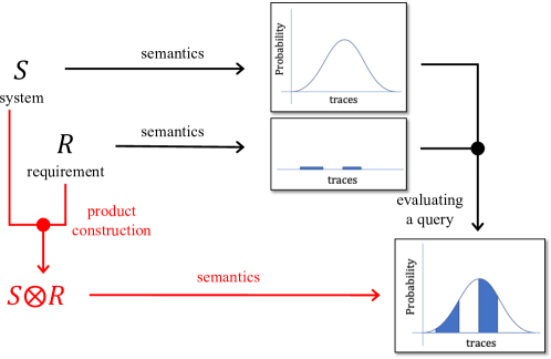
In many situations not only the output distribution is relevant, but also the observable behaviour during execution. In these settings, probabilistic programs describe distributions over system traces, which can be captured as formal languages or time series. Indeed, probabilistic programs are useful to describe the sequential executions of, e.g., network protocols (Smolka et al., 2017, 2019), computer hardware (Roberts et al., 2021), and planning problems (Sanner, 2010). Given a requirement, which describes the desirable traces in a formal language, the problem of temporal inference is then to determine the probability of program traces to meet the requirement (Fig. 1, black).

It is common to specify the requirement as a state machine, which can then be used as a monitor for the requirement to solve the temporal inference problem. However, marginalization of paths to the requirement is not trivial here and a particular challenge of temporal inference in this setting is that naively, the set of system traces is gigantic due to the combinatorial explosion.

Product constructions

Fortunately, even in this setting most temporal inference problems do not actually require analyzing (an approximation of) the full distribution of traces described by the program. Suppose, for instance, that we wish to infer the probability of two successive packets in a network being dropped. For this purpose it suffices to monitor whether the previous packet has been dropped and whether at some point two successive packets have been dropped. All other events that occur during traces can be ignored, leading to a massive reduction of the space of traces.

More generally, to answer a temporal inference query, it suffices to infer the (distribution of the) final status of the monitor, and use this to answer the original query. This powerful idea of analyzing a synchronous composition or product of a system and its monitor is illustrated in Fig. 1 (red). It is a fundamental idea in the verification of linear temporal logics (Pnueli, 1977; Vardi and Wolper, 1986) and has been reapplied for a variety of other properties in quantitative verification, such as resource-bounded reachability (Andova et al., 2003; Laroussinie and Sproston, 2005; Baier et al., 2014a; Hartmanns et al., 2020), timed traces on continuous-time Markov chains (Chen et al., 2009), and conditional probabilities (Baier et al., 2014b). These constructions are derived on a case-by-case basis. Our aim is a generic framework that describes product constructions and sufficient criteria that state for what types of queries inference on these product constructions is correct.

In this work, we assume that operationally, systems are captured by a weighted or probabilistic transition system and the requirement by finite automata. All these types of transitions systems are instances of coalgebras (Jacobs, 2016; Rutten, 2000), which we therefore choose to represent both systems and requirements. At this level of generality, we define a synchronous product of the operational models for (any) system $S$ and requirement $R$. The key idea here is commutation: it does not matter whether we first take the semantics of $S$ and $R$ and adequately combine them, or first take the product of $S$ and $R$ and compute the semantics for this product. The main theorem in this paper formalizes the requirements for which these approaches indeed commute.

A broad framework

Our framework applies to both well-understood and to less studied programs and queries. For probabilistic programs, we support almost-surely terminating programs that describe a distribution over finite traces, and regular specifications captured by DFAs. We also use this construction to support cost-bounded specifications that accumulate cost along every path. The restriction to almost-surely terminating programs can be lifted, and for such programs we support safety properties. Furthermore, our construction is not restricted to probabilistic programs. Indeed, temporal inference on a variety of weighted programs is supported and allows inference on travel costs and optimal resource utilization. We present the list of instances in Fig. 2.

Section System Requirement Inference on Product
Section 3,Section 4 Probabilistic Program that Almost-Surely Terminates RSP Terminating Probability
Section 5 Probabilistic Program with Reward RSP Partial Expected Reward
Section 6 Probabilistic Program that Almost-Surely Terminates Resource Terminating Probability
Section 7 Probabilistic Program that Never Terminates RSP Terminating Probability
Section 8 Weighted Program that Terminates RSP Shortest Path
Section 9 Weighted Program that Terminates Weighted RSP Shortest Path
Figure 2. Instances of coalgebraic inference with coalgebraic product construction. RSP denotes the regular safety property.

A stepping stone towards off-the-shelf temporal inference

The framework provides two algorithmic approaches for temporal inference. First, as a byproduct of our general product construction, we obtain a least fixed point characterization of the solution of a temporal inference problem. This characterization provides value-iteration-like (Puterman, 1994) iterative algorithms to approximate the solution. Furthermore, the fixed point characterization is a stepping stone to apply ideas such as inductive invariants (Kori et al., 2022; Chatterjee et al., 2022; Batz et al., 2023) to answer a variety of queries. Second, the product construction itself corresponds to the operational semantics of some product program, i.e., a program that incorporates the specification and adjusts its return type. These programs are amenable to any approximate or exact inference engine and the correctness of the construction is independent of the correctness of the inference engine. The Rubicon transpiler (Holtzen et al., 2021) exemplifies the creation of such product programs to infer finite-horizon reachability in Dice (Holtzen et al., 2020) programs.

Contributions.

To summarize, this paper presents a unifying framework for probabilistic and weighted temporal inference with temporal properties. Concretely, we contribute

  • a generic definition of temporal inference queries (in Section 3),

  • a generic approach to performing this type of inference, based on a coalgebraic product construction (in Section 4), together with a correctness criterion for this product construction, and

  • case studies of coalgebraic quantitative inference of variable complexity (in Sections 6, 5, 8, 9 and 7).

We use the correctness criterion to recover results on established (Sections 6, 5, 8 and 7) and new (Section 9) temporal inference queries. We start the paper with an overview that illustrates the various types of temporal inference and the product construction. We present related work in Section 10.

Notation

We write $\mathbf{2}$ for the set $\{\top,\bot\}$ of Boolean values. We write $\bot$ for the least element of a partial order, assuming it exists. Let $X$ be a set. The set $\mathcal{P}(X)$ contains the subsets of $X$ and the set $\mathcal{P}^{f}(X)$ the finite subsets of $X$. We write $\mathcal{D}(X)$ for the set of distributions on $X$ whose support is at most countable, and $\mathcal{D}_{\leq 1}(X)$ for the set of subdistributions on $X$ with countable support. For a subdistribution $\nu$, we write $\mathrm{supp}(\nu)$ for the set of supports of $\nu$. We write $\mathbb{N}^{\infty}$ for the set of integers and the positive infinity $\infty$. For a natural number $n\in\mathbb{N}$, we let $[n]:=\{1,\dots,n\}$. We write $(X\rightarrow Y)$ or $Y^{X}$ for the set of functions from $X$ to $Y$. For functions of the form $f\colon X\rightarrow(Y\rightarrow Z)$ we often write $f(x,y)$ instead of $f(x)(y)$, and similarly for functions of the form $P\colon X\rightarrow\mathcal{D}(Y)$ we write $P(x,y)$ instead of $P(x)(y)$. We write $\mathbf{1}_{f=g}$ for the value $1$ if $f=g$ holds, 00 otherwise.

2. Overview

The typical inference task in probabilistic programming languages is to infer (statistics of) the posterior distribution described by the program. In this overview, we highlight probabilistic and weighted programs where we perform inference not on the outcome of the program, but on the executions themselves, which we refer to as temporal inference, and demonstrate how we can use product constructions to reduce the problem to inference on the posterior.

These examples of temporal inference problems motivate the overall challenge addressed in this paper: to give a formal framework that captures the mathematical essence of such product constructions and their use for temporal inference. Moreover, this framework should be flexible and general enough to easily show the correctness of product constructions for a broad range of systems and temporal properties, including the various examples in this overview section.

2.1. Probabilistic Temporal Inference in Probabilistic Programs

Refer to caption
i = 5; j = 3; a = sand;
while (i > 1 or j > 1) {
{i <- max(i-1, 1)} [4/5]
{j <- max(j-1, 1)}
a <- label(i,j);
}

$y_{0}$ $y_{1}$ $y_{2}$ $y_{3}$rechargelakearidlakerecharge,vulcanovulcanovulcano

Figure 3. Robot moves in the $5\times 3$ grid world. The requirement of the robot is given by the DFA. The state $y_{0}$ is the initial state, and $y_{1}$ is the unique accepting state in the DFA. We omit all self-loops for readability.

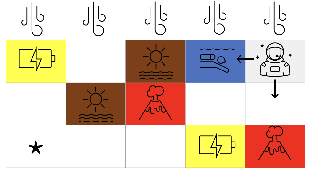
We start with a classical reach-avoid inference task, which we concretize with a robot in a small grid world, inspired by (Vazquez-Chanlatte et al., 2018, 2021). The grid world consists of cells, as displayed in Fig. 3. A cell contains either recharge stations (yellow), lakes (blue), arid areas (brown), or vulcanos (red). All other cells contain nothing but sand (white). As the robot moves, we observe the labels of the cell, which we denote A={sand,recharge,lake,arid,vulcano}𝐴sandrechargelakearidvulcanoA=\{\textsf{sand},\textsf{{\color[rgb]{0.5,0.5,0}\definecolor[named]{pgfstrokecolor}{rgb}{0.5,0.5,0}\pgfsys@color@cmyk@stroke{0}{0}{0.5}{0.5}\pgfsys@color@cmyk@fill{0}{0}{0.5}{0.5}recharge}},{\color[rgb]{0,0,0.5}\definecolor[named]{pgfstrokecolor}{rgb}{0,0,0.5}\textsf{lake}},{\color[rgb]{0.375,0.25,0.125}\definecolor[named]{pgfstrokecolor}{rgb}{0.375,0.25,0.125}\textsf{arid}},{\color[rgb]{0.5,0,0}\definecolor[named]{pgfstrokecolor}{rgb}{0.5,0,0}\textsf{vulcano}}\}. Any finite sequence of areas is thus representable in $A^{+}$. We consider the case where the robot follows a fixed plan that describes in every cell what direction it aims to go. However, the actual outcome of trying to move in that direction is probabilistic, due to, e.g., wind gusts from the north.111More realistic examples in probabilistic robots show that the outcome of an actuator action is often uncertain.

The (simplified) probabilistic program described in Fig. 3 is a possible implementation of the robot movement. The robot starts at $\langle i=5,j=3\rangle$, which is a sand cell. As long as the robot has not reached the lower left corner, it will move left with probability $\frac{4}{5}$ and move down otherwise. We explicitly store the label of the current cell with a function label which returns this label. We remark that this program almost-surely terminates — we consider programs that do not necessarily almost-surely terminate later in this section. The program then induces a distribution $\nu\in\mathcal{D}(A^{+})$ over traces which represent paths that the robot takes.

The aim of the robot is to reach a charging station, but this is subject to some rules: the robot should never travel over vulcanos; a wet robot should not recharge; a robot becomes wet when travelling through lakes; and a robot becomes dry when travelling through arid areas. Formally, these rules can be captured as a set $L\subseteq A^{+}$ of safe paths, which we refer to as the requirement. Such requirements can be encoded using regular expressions or using temporal logics such as (fragments of) (finitary) LTL. In this example, we assume that the requirement $L$ is given by a deterministic finite automaton (DFA) as in Fig. 3.

Generally, we want to find the probability that a trace generated by the program belongs to the set of traces specified in the requirement. More precisely, let $\nu\in\mathcal{D}(A^{+})$ be the trace distribution generated by the program and $L\subseteq A^{+}$ (or equivalently, $L\in\mathcal{P}({A}^{+})$) the language represented by the DFA for the requirement. Formally, our aim is to answer a (temporal) inference query, namely to compute $q(\nu,L)$ in:

$$q_{\mathsf{prob}}\colon\mathcal{D}(A^{+})\times\mathcal{P}({A}^{+})\rightarrow[0,1],\quad\text{where}\quad\!q_{\mathsf{prob}}(\nu,L)\coloneq\sum_{w\in L}\nu(w).$$

Such inference queries are heavily studied in the area of probabilistic model checking (Baier et al., 2018).222Model checking would typically define a models relation $\models$ such that, e.g., $\nu\models L$ if $q(\nu,L)\geq\frac{1}{2}$. Towards efficient inference, the key aim is to avoid computing $\nu$ and $L$ first, as the set $A^{+}$ is (countably) infinite. Instead, the standard approach is to construct a product of the operational semantics of the program and the requirement, given as a Markov chain (MC) and a DFA, respectively.

We give concrete (but simplified) operational semantics333The operational semantics of probabilistic programs can be defined as a Markov chain that includes the assignment to the variables but also the program counter (Gretz et al., 2014). We omit the program counter for simplicity. for the program in Fig. 3. The program halts in a dedicated state $\star$. The operational semantics is an MC with state labels, referred to below as the system. Formally, it is defined using (regular) states $X=\{(i,j)\mid i\in[1,5],j\in[1,3],(i>1\text{ or }j>1)\}$ where $[1,m]$ is the set $\{1,\dots,m\}$, terminating state $\star$, labels A={sand,recharge,lake,arid,vulcano}𝐴sandrechargelakearidvulcanoA=\{\textsf{sand},\textsf{{\color[rgb]{0.5,0.5,0}\definecolor[named]{pgfstrokecolor}{rgb}{0.5,0.5,0}\pgfsys@color@cmyk@stroke{0}{0}{0.5}{0.5}\pgfsys@color@cmyk@fill{0}{0}{0.5}{0.5}recharge}},{\color[rgb]{0,0,0.5}\definecolor[named]{pgfstrokecolor}{rgb}{0,0,0.5}\textsf{lake}},{\color[rgb]{0.375,0.25,0.125}\definecolor[named]{pgfstrokecolor}{rgb}{0.375,0.25,0.125}\textsf{arid}},{\color[rgb]{0.5,0,0}\definecolor[named]{pgfstrokecolor}{rgb}{0.5,0,0}\textsf{vulcano}}\}, initial state $(5,3)$, and the transition probability $P\colon X\rightarrow\mathcal{D}(X+\{\star\})$ with for $i>1$ or $j>1$,

$\displaystyle P\big{(}(i,j)\big{)}\big{(}(i^{\prime},j^{\prime})\big{)}$ $\displaystyle\coloneq\begin{cases}\frac{4}{5}&\text{ if $i^{\prime}=\mathrm{max}(i-1,\,1)$ and $j^{\prime}=j$,}\\ \frac{1}{5}&\text{ if $i^{\prime}=i$ and $j^{\prime}=\mathrm{max}(j-1,\,1)$,}\\ 0&\text{ otherwise.}\end{cases}$

Here, we regard the terminating state $\star$ as the grid $(1,1)$ in order to make the definition simpler.

Similarly, the DFA shown in Fig. 3, consists of states $Y=\{y_{0},y_{1},y_{2},y_{3}\}$, a set of accepting states $F=\{y_{3}\}$ and a labelled transition relation $T\subseteq Y\times A\times Y$ as indicated by the arrows in Fig. 3.

From the system and the requirement, the product construction yields a transition system whose states are pairs of states of the system and the requirement, and whose transitions are “synchronized” transitions. In this product, the labels do not explicitly appear anymore. Concretely, the product of the MC and the DFA given above is again a Markov chain, with two semantically different terminal states, i.e., the state space is $X\times Y+\mathbf{2}$. States are thus either a tuple of an MC state and DFA state, or a Boolean flag, which is used to indicate whether upon reaching $\star$ the execution is accepted by the DFA. For the original transition matrix $P$, we can define the new transition matrix $P^{\prime}$, using $[x]=\top$ iff $x$ evaluates to true, as follows:

$\displaystyle P^{\prime}\big{(}(x,y),\,(x^{\prime},y^{\prime})\big{)}$ $\displaystyle\coloneq\begin{cases}P\big{(}x,\,x^{\prime}\big{)}&\text{ if }(y,L(x^{\prime}),y^{\prime})\in T,\\ 0&\text{ otherwise,}\end{cases}$
$\displaystyle P^{\prime}\big{(}(x,y),\,[y\in F]\big{)}$ $\displaystyle\coloneq P\big{(}x,\,\star\big{)}.$

The temporal inference problem for the robot can now be answered by asking the probability of terminating while accepting, i.e., of reaching the state $\top$ or equivalently of returning $\top$. This probability coincides with $q(\nu,L)$ by construction as it keeps track of the path for reaching $\star$ is in $L$. Thus, the product construction enables temporal inference by applying inference methods that analyze the distribution of outputs from the product.

The essence of tractable solutions to temporal inference is to construct a synchronous product of the program and the requirement.

In the example above, the product of a MC with a terminal state and a DFA yields an MC with two terminal states (one accepting, one rejecting). There are thus three types of transition systems involved. We therefore propose to use coalgebras as a generic approach to describe transition systems of different types. A key challenge in this paper is that the type of the product transition system also varies, depending on the system, the requirement and the query itself. As we highlight in examples below, this essence reappears in a variety of temporal inference queries. We later show how the inference problem Section 3 and product construction Section 4 fits into our framework.

Markov chains and DFAs as coalgebras

Coalgebraically, we can capture an MC with a terminal state by a single function: $c\colon X\rightarrow\mathcal{D}(X+\{\star\})\times{A}$ given by $c(x)\coloneq\big{(}P(x),L(x)\big{)}$. We ignore the initial state in this representation. We present DFAs as coalgebras of the form $d\colon Y\rightarrow(Y\times\mathbf{2})^{A}$, where $Y$ is the set of states, and $A$ are the labels of the grids. Note that output is on transitions, as in Mealy machines; for each state $y\in Y$ and status $a\in A$, the value $b\in\mathbf{2}$ given by $(y^{\prime},b)\coloneq d(y)(a)$ is $\top$ if $y^{\prime}$ is the accepting state, i.e., $y^{\prime}=y_{1}$, and $\bot$ otherwise. The product transition system then has type $c\otimes d\colon X\times Y\rightarrow\mathcal{D}\big{(}X\times Y+\mathbf{2}\big{)}$. We write $\big{(}c\otimes d\big{)}\big{(}(x,y),\,(x^{\prime},y^{\prime})\big{)}$ instead of $\big{(}c\otimes d\big{)}\big{(}(x,y))((x^{\prime},y^{\prime})\big{)}$.

2.2. Extended Probabilistic Temporal Inference Queries

There exist plenty of inference queries where the requirement or query changes.

Partial expected rewards

Almost classical are partial expected rewards (rewards are also often referred to as costs) (Baier and Katoen, 2008; Baier et al., 2017). They have been studied, for instance, to determine the expected runtime of randomized algorithms (Kaminski et al., 2018). In terms of the earlier example, we may annotate every state with additional movement time that depends, e.g., on the type of surface. As a coalgebra, we would describe the system as $c\colon X\rightarrow\mathcal{D}(X+\{\star\})\times{\mathbb{N}\times A}$, i.e., with integer movement cost. A natural query is to ask what the expected arrival time is upon reaching a recharge station. In that case, the requirement remains the same DFA as above, which accepts the safe paths including a recharge station. As before, a query takes the system and the requirement, but is now defined to compute the weighted sum of probability times reward. We continue this discussion in Section 5.

Reward-bounded reachability

Rather than inferring the expected time to reach a cell, it is often relevant to determine the probability to reach a cell before some deadline. This is particularly relevant for limited resources, such as battery levels, where we want to compute the probability to reach a recharge station before the battery is empty or, in a different scenario, to compute the probability to reach the airport before a flight departs. These scenarios are instances of cost-bounded reachability problems (Andova et al., 2003; Baier et al., 2014a; Hartmanns et al., 2020). Intuitively, every path gets a finite resource cost, and we are interested in analyzing the probability that we obtain a path that meets a threshold on the cost of this path. Here, the main observation that is necessary is to realize that this requirement can be captured by finite automata. In fact, also more general notions with the potential to recharge the batteries, as formally captured using consumption Markov chains (Blahoudek et al., 2021) can be supported, see Section 6.

Conditional probabilities

We want to highlight that the provided queries can be building blocks towards even more generic queries. For example, conditional probability queries help to restrict a model to the behavior that corresponds to a set of observations. They can be supported using Bayes’ rule. Formally, the following query supports analyzing the probability of satisfying a requirement $L$ conditioned on satisfying a conditional observation $C$.

$$q_{\textsf{cond}}\colon\mathcal{D}(A^{+})\times\mathcal{P}({A}^{+})\times\mathcal{P}({A}^{+})\rightarrow[0,1],\quad q_{\textsf{cond}}(\nu,L,C)\coloneq\frac{q_{\mathsf{prob}}(\nu,L\cap C)}{q_{\mathsf{prob}}(\nu,C)}=\frac{\sum_{w\in L\cap C}\nu(w)}{\sum_{w\in C}\nu(w)},$$

where $q_{\mathsf{prob}}$ is the query from Section 2.1. The query can be used to define the probability that we reach a charging station conditioned on reaching an arid field. The partial expected rewards can also be used to compute conditional rewards, which will be clarified in Section 5.

Remark 2.1.

We assume here that the conditioning is given separately from the system. Many probabilistic programs allow to explicitly formulate the conditioning inside the program using observe statements (Olmedo et al., 2018). However, such programs can be seen as formulating both a distribution over paths (without conditioning) and a set of paths to use for conditioning.

2.3. Probabilistic Temporal Inference for Programs that do not Terminate

x = 5; y = 3; a = sand;
while (true) {
{x <- max(x-1,0)} [1/4] {y <- max(y-1,0)} [1/4]
{x <- min(x+1,5)} [1/4] {y <- min(y+1,3)};
a <- label(x,y);
}

$y_{0}$ $y_{1}$ $y_{2}$rechargevulcanoA{recharge,vulcano}𝐴rechargevulcanoA\setminus\{\textsf{{\color[rgb]{0.5,0.5,0}\definecolor[named]{pgfstrokecolor}{rgb}{0.5,0.5,0}\pgfsys@color@cmyk@stroke{0}{0}{0.5}{0.5}\pgfsys@color@cmyk@fill{0}{0}{0.5}{0.5}recharge}},{\color[rgb]{0.5,0,0}\definecolor[named]{pgfstrokecolor}{rgb}{0.5,0,0}\textsf{vulcano}}\}$A$ $A$

Figure 4. Reactive gridworld: Robot moves in the $5\times 3$ grid world in any direction, the program never halts. The requirement expresses that we want to reach a charging station without reaching a vulcano.

Above, we considered programs that almost-surely terminate. However, it is often useful to describe models that do not terminate. For instance, the program in Fig. 4 never halts: The robot continuously moves throughout the grid. Still, it is natural to ask for the probability of eventually reaching a charging station without reaching a vulcano before. We give this requirement using a simple DFA that captures the (finite, unbounded) executions that satisfy the requirement. We note that we are thus interested in paths that have a finite (but unbounded) prefix in the requirement, i.e., we consider regular safety properties.

Since the traces of the robot are now infinite, we need (limited) measure-theoretic tools, in particular, a cylinder set construction (Baier and Katoen, 2008). Consequentially, the query no longer takes a distribution over finite paths, but a specific $\sigma$-algebra as first argument. However, while the ingredients become more involved, the generic framework from before still applies. We formalize the construction in Section 7. We also show how we can express the inference in programs that almost-surely terminate to programs that never halt.

2.4. Inference Queries for Weighted Programs

We now consider a type of quantitative temporal inference different from the probabilistic examples. Weighted Programming (Cohen et al., 2011; Brunel et al., 2014; Gaboardi et al., 2021; Batz et al., 2022; Belle and Raedt, 2020) is an emerging paradigm that aims to model mathematical problems using syntax and semantics from programming languages. Probabilistic programs are a special instance of weighted programs where we multiply probabilities along paths and then sum over all paths. Weighted programs allow to parameterize the operations along paths and over all paths.

One instance of weighted programs is formed by optimization problems that attempt to minimize the costs expressed as weights along traces. Formally, these program use the tropical semiring $(\mathbb{N}^{\infty}=\mathbb{N}+\{\infty\},\min,+)$ to combine minimization and addition over the extended natural numbers: the program minimizes over all traces while summing the costs along the traces. We are interested in temporal inference that encodes a constrained optimization variant, in which we minimize only over traces that satisfy a given requirement.

t: town; nt: town, a: action;
t = "hometown";
min{
while (t != "destination") {
(nt, a) in possible_choice(t);
add{t <- move(nt, a)};
}
}
(a) Traveler’s move.

$y_{0}$ $y_{1}$TP,  B,  T

(b) Requirement $(\dagger)$.
Figure 5. Travelling problem. The functions ${\color[rgb]{1,.5,0}\definecolor[named]{pgfstrokecolor}{rgb}{1,.5,0}\mathrm{min}}$ and ${\color[rgb]{1,.5,0}\definecolor[named]{pgfstrokecolor}{rgb}{1,.5,0}\mathrm{add}}$ in the weighted program are the primary operations on the costs (or weights in general). The state $y_{0}$ is the initial state, and $y_{1}$ is the unique accepting state in the NFA $d$. The characters $\mathrm{P},\mathrm{B},\mathrm{T}$ correspond to taking a plane, a bus, and a train, respectively.

We exemplify the problem statement with a simple planning problem: the Travelling Problem. A scientist is about to leave home to travel to a conference using a variety of potential transportation means. The weighted program in Fig. 5(a) models the transfer of the scientist; traces of the program correspond to transfer histories, and fares along traces are accumulated as total costs. The scientist can provide a requirement with personal preferences. The scientist loves taking trains and wants to arrive by train at the destination $(\dagger)$. The nondeterministic finite automaton (NFA) in Fig. 5 captures this simple requirement.

The travelling problem can be formulated as the following temporal inference query: let (i) $T\in\mathcal{P}(A^{+}\times\mathbb{N})$ be the set of pairs $(w,m)$ of a trace $w\in A^{+}$ and a possible accumulated cost $m\in\mathbb{N}$ along the trace $w$, and (ii) $L\in\mathcal{P}({A}^{+})$ be the recognized language of the NFA. The inference query

$\displaystyle q\colon\mathcal{P}(A^{+}\times\mathbb{N})\times\mathcal{P}({A}^{+})\rightarrow\mathbb{N}^{\infty},\quad q(T,L)\coloneq\min\{m\mid w\in L,\,(w,m)\in T\}.$

naturally formalizes the requested quantity. However, computing the value $q(T,L)$ is not trivial as the sets $A^{+}$ and $\mathbb{N}$ are countably infinite.

The key to solving the Travelling Problem again lies in the construction of a product of the operational semantics of the program and the requirement, in a similar style to Section 2.1. The operational semantics of the weighted program shown in Fig. 5(a) is the weighted transition system $c\colon X\rightarrow\mathcal{P}\big{(}(X+\{\star\})\times A\times[M]\big{)}$, where (i) $X$ is the set of towns that can be used to transfer; (ii) $\star$ represents the destination; (iii) $A$ is the set of means of transport; and (iv) $[M]=\{1,\dots,M\}$ is the set of costs. For each town $x\in X$, the set $c(x)$ contains triples $(x^{\prime},a,m)$ where $x^{\prime}$ is the next town, $a$ its means of transport, and $m$ the associated cost. Requirements are captured by NFAs. As before, we take a variant of NFAs with output on transitions and formalize them as coalgebras of the form $d\colon Y\rightarrow\big{(}\mathcal{P}(Y\times\mathbf{2})\big{)}^{A}$, where $\mathbf{2}$ represents whether the next reaching state is accepting or not.

Then, the product $c\otimes d$ of the operational semantics of the program $c$ and the requirement $d$ is the “synchronized” transition system, which has the type $c\otimes d\colon X\times Y\rightarrow\mathcal{P}\big{(}(X\times Y+\mathbf{2})\times[M]\big{)}$. The Travelling Problem can then be solved as a simple shortest path problem on the product $c\otimes d$. Again, the product construction leads to an efficient solution by disregarding the individual steps. In Section 8 we show how weighted temporal inference fits into our framework.

In the Traveling Problem above, the costs are completely determined by the system. In fact, it is possible to add additional costs via the requirement. That can be used to penalize certain travel options and allows for additional flexibility for the user to specify constraints. We show such a generalization in Section 9.

2.5. Towards a Unifying Theory of Product Constructions

The range of quantitative temporal inference problems discussed above are broad, but share a common pattern: there is an underlying product construction which we may use to efficiently solve the original temporal inference problem. The challenge we address is to identify the mathematical essence of product constructions and their role in practical solutions for temporal inference. More precisely, let $\llbracket\cdot\rrbracket_{c}$ be the semantics of the system (e.g., an MC with labels), $\llbracket\cdot\rrbracket_{d}$ the semantics of the requirement (e.g., a DFA or an NFA), and let $\llbracket\cdot\rrbracket_{c\otimes d}$ of the product (e.g., an MC without labels); and let $q$ be the temporal inference query of interest. We aim for the following equality that states the “correctness” of the product for temporal inference:

(1) $$\llbracket x,y\rrbracket_{c\otimes d}=q(\llbracket x\rrbracket_{c}\times\llbracket y\rrbracket_{d}).$$

This equality is the starting point for our main question: How can we uniformly construct a product $c\otimes d$ from a system $c$ and a requirement $d$ and ensure that Eq. 1 holds? Towards an answer, we use coalgebras (see, e.g., (Jacobs, 2016)) as the foundation for our theory of temporal inference and product constructions. The theory of coalgebras provides us with a generic expression of transition systems that covers a wide variety of system types and a way of defining their semantics as least fixed points of suitable predicate transformers.

The theory of coalgebras is general enough to define both weighted and probabilistic systems, and requirements, which are often variations of finite automata. We observe that a product between system and requirement is induced by a distributive law between functors—these have been widely studied in, for instance, the theory of programming languages (e.g. (Turi and Plotkin, 1997; Aguirre and Birkedal, 2023; Goncharov et al., 2023)), and automata theory (e.g. (Jacobs, 2006; Silva et al., 2013; Jacobs et al., 2015; Klin and Rot, 2016)). This formulation naturally leads us to a definition of correctness, formalising Eq. 1. Our main result is a sufficient condition for correctness, referred to as our correctness criterion (Thm. 4.6). As we show in the second part of this paper, this simple theorem is powerful enough to cover a variety of temporal inference problems, including all examples discussed above.

3. Coalgebraic Inference

In this section, we introduce a generic framework, called coalgebraic inference, which unifies the temporal inference problems shown in the previous section. This framework relies on the generality of coalgebras as a mathematical notion of state-based system: we model both systems and requirements as coalgebras, and define the notion of query in this context.

3.1. Generic Semantics of Coalgebras

Intuitively, a coalgebra maps states $X$ to $F(X)$, which is a set that specifies (i) the type of transition, e.g., probabilistic or non-deterministic, and (ii) the information of a state $x\in X$, e.g., a label $a$ or a weight $m\in\mathbb{N}$ assigned to $x$. In $F(X)$, $F$ is a functor:

Definition 3.1 (functor).

A functor $F$ maps sets $X$ to sets $F(X)$ and functions $f\colon X\rightarrow Y$ to functions $F(f)\colon F(X)\rightarrow F(Y)$, such that:

  • $F$ preserves identities, i.e., for any set $X$, $F(\mathrm{id}_{X})=\mathrm{id}_{F(X)}$,

  • $F$ preserves composition, i.e., for functions $f\colon X\rightarrow Y$ and $g\colon Y\rightarrow Z$, $F(g\circ f)=F(g)\circ F(f)$.

Definition 3.2 (coalgebra).

A coalgebra for a functor $F$ and states $X$ is a function $c\colon X\rightarrow F(X)$.

Example 3.3 (coalgebras).

We list some coalgebras discussed in this paper:

  1. (1)

    A (labeled) Markov chain (MC) with a target state $\star$ is a pair of functions $(P,\,L)$, where $P\colon X\rightarrow\mathcal{D}{(X+\{\star\})}$ captures the probabilistic transitions, and $L\colon X\rightarrow A$ is a labelling of states. A Markov chain $(P,\,L)$ is indeed a coalgebra $c\colon X\rightarrow\mathcal{D}(X+\{\star\})\times{A}$ given by $c(x)\coloneq\big{(}P(x),\,L(x)\big{)}$ for each $x\in X$.

    The underlying functor $F$ is defined on a set $X$ by $F(X)=\mathcal{D}(X+\{\star\})\times{A}$. For a function $f\colon X\rightarrow Y$, the function $F(f)\colon F(X)\rightarrow F(Y)$ informally replaces all occurrences of elements $x\in X$ by $f(x)$, yielding again a distribution. More precisely, $F(f)(\nu_{X},a)=(\nu_{Y},a)\in\mathcal{D}(Y+\{\star\})\times{A}$ where $\nu_{Y}(y)\coloneq\sum_{x\in f^{-1}(y)}\nu_{X}(x)$, and $\nu_{Y}(\star)\coloneq\nu_{X}(\star)$.

  2. (2)

    A deterministic finite automaton (DFA) is a coalgebra $d\colon Y\rightarrow(Y\times\mathbf{2})^{A}$, where the underlying set $Y$ is finite. We note that the acceptance label is assigned to transitions, which can encode the standard definition where the acceptance label is assigned to states.

  3. (3)

    A Markov chain without the target state $\star$ is a coalgebra $c\colon X\rightarrow\mathcal{D}(X)\times{A}$.

  4. (4)

    A weighted transition system is a coalgebra $c\colon X\rightarrow\mathcal{P}\big{(}(X+\{\star\})\times A\times\mathbb{N}\big{)}$, where each non-deterministic transition provides a pair $(a,m)\in A\times\mathbb{N}$ of the label $a$ and the weight $m$.

We use a generic notion of semantics of coalgebras, characterised by a semantic domain and a modality. Examples of semantic domains in this paper are sub-distributions over traces, and languages over a fixed alphabet. We illustrate the modalities in examples below.

Definition 3.4 (semantic structure, predicate transformer).

A semantic structure for a functor $F$ is a tuple of an $\omega$-cpo444 see Appendix A for the definition of $\omega$-cpos $\mathbf{\Omega}\coloneq(\Omega,\preceq)$ and a modality $\tau\colon F(\Omega)\rightarrow\Omega$. We refer to an element $v\in\Omega$ as a semantic value. Given a coalgebra $c\colon X\rightarrow F(X)$, the induced predicate transformer $\Phi_{\tau,c}\colon\Omega^{X}\rightarrow\Omega^{X}$ is given by

$$\Phi_{\tau,c}(u)\coloneq\tau\circ F(u)\circ c.$$

If $\tau$ and $c$ are clear from the context we write $\Phi$ instead of $\Phi_{\tau,c}$.

Inducing predicate transformers by modalities is a standard technique in coalgebraic modal logic (e.g. (Kupke and Pattinson, 2011)). Informally, modalities explain how to combine semantic values of successor states into a single semantic value of the current state. For instance, for an unlabeled MC, we can take a semantic domain $\Omega$ as $[0,1]$. The reachability probability from the current state is computed by a weighted sum over the reachability probabilities from the successor states; this is modeled by the modality $\tau$. In a labeled MC, the semantic domain is the set $\mathcal{D}_{\leq 1}({A}^{+})$ of subdistributions over traces; we show this in Ex. 3.6. Throughout the paper, we only consider $\omega$-continuous predicate transformers $\Phi$.

Definition 3.5 (semantics of coalgebras).

Let $\Phi_{\tau,c}$ as above be an ($\omega$-continuous) predicate transformer. The semantics of the coalgebra $c$ is the least fixed point $\llbracket\cdot\rrbracket_{c}\colon X\rightarrow\Omega$ of $\Phi_{\tau,c}$ in Eq. 2.

(2) ${F(X)}$ ${F(\Omega)}$ ${X}$ ${\Omega}$ $\scriptstyle{F(\llbracket\cdot\rrbracket_{c})}$ ${=_{\mu}}$ $\scriptstyle{\tau}$ $\scriptstyle{c}$ $\scriptstyle{\llbracket\cdot\rrbracket_{c}}$

As $\Phi$ is $\omega$-continuous on $\omega$-cpo $\mathbf{\Omega}$, the least fixed point $\llbracket\cdot\rrbracket_{c}$ exists, and can be computed as the join $\bigvee_{n\in\mathbb{N}}\Phi^{n}(\bot)$, by the Kleene fixed point theorem (Cousot and Cousot, 1979; Baranga, 1991).

${\mathcal{D}(X+\{\star\})\times{A}}$ ${\mathcal{D}(\mathcal{D}_{\leq 1}({A}^{+})+\{\star\})\times{A}}$ ${X}$ ${\mathcal{D}_{\leq 1}({A}^{+})}$ $\scriptstyle{\mathcal{D}(\llbracket\cdot\rrbracket_{c}+\{\star\})\times{A}}$ ${=_{\mu}}$ $\scriptstyle{\tau_{S}}$ $\scriptstyle{c}$ $\scriptstyle{\llbracket\cdot\rrbracket_{c}}$
Figure 6. The semantics $\llbracket\cdot\rrbracket_{c}$ of a Markov chain (MC) $c\colon X\rightarrow\mathcal{D}(X+\{\star\})\times{A}$, where $\Phi(u)\coloneq\tau_{S}\circ\mathcal{D}(u+\{\star\})\times{A}\circ c$.
$x_{0},\textsf{sand}$ $x_{1},{\color[rgb]{0,0,0.5}\definecolor[named]{pgfstrokecolor}{rgb}{0,0,0.5}\textsf{lake}}$ $x_{2},\textsf{sand}$x3,rechargesubscript𝑥3rechargex_{3},\textsf{{\color[rgb]{0.5,0.5,0}\definecolor[named]{pgfstrokecolor}{rgb}{0.5,0.5,0}\pgfsys@color@cmyk@stroke{0}{0}{0.5}{0.5}\pgfsys@color@cmyk@fill{0}{0}{0.5}{0.5}recharge}}$x_{4},{\color[rgb]{0.5,0,0}\definecolor[named]{pgfstrokecolor}{rgb}{0.5,0,0}\textsf{vulcano}}$ $\star$ $\frac{4}{5}$ $\frac{1}{5}$ $1$ $\frac{4}{5}$ $\frac{1}{5}$ $1$ $1$
$y_{0}$ $y_{1}$ $y_{2}$ $y_{3}$rechargelakearidlakerecharge,vulcanovulcanovulcano
Figure 7. A (small) MC (on the left) and the DFA shown in Fig. 3 (on the right).

We exemplify such semantics for MCs and for DFAs. As running examples, we use (i) the MC presented in Fig. 7, which is a small variant of the MC in Fig. 3 with the same transition probabilities, and (ii) the DFA shown in Fig. 7 ( and also in Fig. 3).

Example 3.6 (MC).

We expect that the semantics from any state $s_{1}$ is the distribution $\sigma\in\mathcal{D}(A^{+})$ over the traces that eventually reach the target state $\star$. For instance, the semantics $\sigma$ of the MC in Fig. 7, from the initial state, should be the distribution given by

sandlakerecharge4/5,sandsandrecharge4/25,sandsandvulcano1/25.formulae-sequencemaps-tosandlakerecharge45formulae-sequencemaps-tosandsandrecharge425maps-tosandsandvulcano125\textsf{sand}\cdot{\color[rgb]{0,0,0.5}\definecolor[named]{pgfstrokecolor}{rgb}{0,0,0.5}\textsf{lake}}\cdot\textsf{{\color[rgb]{0.5,0.5,0}\definecolor[named]{pgfstrokecolor}{rgb}{0.5,0.5,0}\pgfsys@color@cmyk@stroke{0}{0}{0.5}{0.5}\pgfsys@color@cmyk@fill{0}{0}{0.5}{0.5}recharge}}\mapsto\nicefrac{{4}}{{5}},\quad\textsf{sand}\cdot\textsf{sand}\cdot\textsf{{\color[rgb]{0.5,0.5,0}\definecolor[named]{pgfstrokecolor}{rgb}{0.5,0.5,0}\pgfsys@color@cmyk@stroke{0}{0}{0.5}{0.5}\pgfsys@color@cmyk@fill{0}{0}{0.5}{0.5}recharge}}\mapsto\nicefrac{{4}}{{25}},\quad\textsf{sand}\cdot\textsf{sand}\cdot{\color[rgb]{0.5,0,0}\definecolor[named]{pgfstrokecolor}{rgb}{0.5,0,0}\textsf{vulcano}}\mapsto\nicefrac{{1}}{{25}}.

We show how to present this semantics of MCs as coalgebraic semantics. Let $c\colon X\rightarrow\mathcal{D}(X+\{\star\})\times{A}$, and $c(x)=\big{(}P(x),L(x)\big{)}$ for $x\in X$. Formally, for each $x\in X$ and $w\in A^{+}$, the semantics $\sigma(x)(w)$ is inductively given by

$\displaystyle\sigma(x)(w)\coloneq\begin{cases}P(x,\star)&\text{ if $w=L(x)$},\\ \sum_{x^{\prime}\in X}P(x,x^{\prime})\cdot\sigma(x^{\prime})(w^{\prime})&\text{ if $w=L(x)\cdot w^{\prime}$},\\ 0&\text{ otherwise. }\end{cases}$

This semantics can indeed be obtained as an instance of Def. 3.4. Consider the semantic structure $S=(\mathbf{\Omega}_{S},\tau_{S})$, where the semantic domain $\mathbf{\Omega}_{S}$ is given by $\Omega_{S}\coloneq\mathcal{D}_{\leq 1}({A}^{+})$, ordered pointwise555$\nu_{1}\preceq\nu_{2}$ if $\nu_{1}(w)\leq\nu_{2}(w)$ for any $w\in A^{+}$, and the modality $\tau_{S}\colon\mathcal{D}(\mathcal{D}_{\leq 1}({A}^{+})+\{\star\})\times{A}\rightarrow\mathcal{D}_{\leq 1}({A}^{+})$ is given by

$$\tau_{S}(\nu,a)(w)\coloneq\begin{cases}\nu(\star)&\text{ if }w=a,\\ \sum_{\nu^{\prime}\in\mathrm{supp}(\nu)\cap\mathcal{D}_{\leq 1}({A}^{+})}\nu(\nu^{\prime})\cdot\nu^{\prime}(w^{\prime})&\text{ if }w=a\cdot w^{\prime},\\ 0&\text{ otherwise. }\end{cases}$$

This modality $\tau_{S}$ can be exemplified as follows. Consider two distribution over traces,

ν1:lakerecharge1,ν2:sandrecharge4/5,sandvulcano1/5:subscript𝜈1maps-tolakerecharge1subscript𝜈2:formulae-sequencemaps-tosandrecharge45maps-tosandvulcano15\displaystyle\nu_{1}\colon{\color[rgb]{0,0,0.5}\definecolor[named]{pgfstrokecolor}{rgb}{0,0,0.5}\textsf{lake}}\cdot\textsf{{\color[rgb]{0.5,0.5,0}\definecolor[named]{pgfstrokecolor}{rgb}{0.5,0.5,0}\pgfsys@color@cmyk@stroke{0}{0}{0.5}{0.5}\pgfsys@color@cmyk@fill{0}{0}{0.5}{0.5}recharge}}\mapsto 1,\qquad\nu_{2}\colon\textsf{sand}\cdot\textsf{{\color[rgb]{0.5,0.5,0}\definecolor[named]{pgfstrokecolor}{rgb}{0.5,0.5,0}\pgfsys@color@cmyk@stroke{0}{0}{0.5}{0.5}\pgfsys@color@cmyk@fill{0}{0}{0.5}{0.5}recharge}}\mapsto\nicefrac{{4}}{{5}},\quad\textsf{sand}\cdot{\color[rgb]{0.5,0,0}\definecolor[named]{pgfstrokecolor}{rgb}{0.5,0,0}\textsf{vulcano}}\mapsto\nicefrac{{1}}{{5}}

which correspond to the semantics of $x_{1},x_{2}$, respectively. Now consider $\nu\colon\nu_{1}\mapsto\nicefrac{{4}}{{5}},\nu_{2}\mapsto\nicefrac{{1}}{{5}}$, which can be intuitively mapped to state $x_{0}$. The modality helps us to construct the semantics for $x_{0}$ from $\nu$, i.e., from the semantics for the successors of $x_{0}$, via the induced predicate transformer $\Phi$ on $\mathcal{D}_{\leq 1}({A}^{+})^{X}$, which is given by

$$\Phi(u)(x)(w)\coloneq\begin{cases}P(x,\star)&\text{ if $w=L(x)$, }\\ \sum_{x^{\prime}\in X}P(x,x^{\prime})\cdot u(x^{\prime},w^{\prime})&\text{ if $w=L(x)\cdot w^{\prime}$,}\\ 0&\text{ otherwise, }\end{cases}$$

for each $u\colon X\rightarrow\mathcal{D}_{\leq 1}({A}^{+})$, $x\in X$ and $w\in A^{+}$. Then, for each $x\in X$, the coalgebraic semantics $\llbracket x\rrbracket_{c}$ shown in Fig. 6 is exactly the semantics $\sigma(x)$ defined concretely above.

Example 3.7 (DFA).

We expect that the semantics of a state of a DFA is its recognized language $L\in\mathcal{P}({A}^{+})$ excluding the empty string $\epsilon$. Concretely, the semantics of the DFA shown in Fig. 3 represents the requirement for the robot, discussed before. For example, the semantics includes the trace w2=sandsandrechargesubscript𝑤2sandsandrechargew_{2}=\textsf{sand}\cdot\textsf{sand}\cdot\textsf{{\color[rgb]{0.5,0.5,0}\definecolor[named]{pgfstrokecolor}{rgb}{0.5,0.5,0}\pgfsys@color@cmyk@stroke{0}{0}{0.5}{0.5}\pgfsys@color@cmyk@fill{0}{0}{0.5}{0.5}recharge}}, but does not include the trace w1=sandlakerechargesubscript𝑤1sandlakerechargew_{1}=\textsf{sand}\cdot{\color[rgb]{0,0,0.5}\definecolor[named]{pgfstrokecolor}{rgb}{0,0,0.5}\textsf{lake}}\cdot\textsf{{\color[rgb]{0.5,0.5,0}\definecolor[named]{pgfstrokecolor}{rgb}{0.5,0.5,0}\pgfsys@color@cmyk@stroke{0}{0}{0.5}{0.5}\pgfsys@color@cmyk@fill{0}{0}{0.5}{0.5}recharge}}. We formulate this semantics for (coalgebraic) DFAs. Let $d\colon Y\rightarrow(Y\times\mathbf{2})^{A}$ be a DFA. Formally, for each $y\in Y$, the semantics $L(y)\colon A^{+}\rightarrow\mathbf{2}(\cong\mathcal{P}({A}^{+}))$ is inductively given by

$\displaystyle L(y)(w)\coloneq\begin{cases}\top&\text{ if $w=a$ and $d(y,a)=(\_,\top)$},\\ &\text{ or $w=a\cdot w^{\prime}$, $d(y,a)=(y^{\prime},\_)$, and $L(y^{\prime})(w^{\prime})=\top$, }\\ \bot&\text{ otherwise.}\end{cases}$

This is recovered through the semantic structure $R=(\mathbf{\Omega}_{R},\tau_{R})$, where the semantic domain $\mathbf{\Omega}_{R}$ is given by $\Omega_{R}\coloneq\mathcal{P}({A}^{+})$, and $T_{1}\preceq T_{2}$ if $T_{1}\subseteq T_{2}$ and the modality $\tau_{R}\colon(\mathcal{P}({A}^{+})\times\mathbf{2})^{A}\rightarrow\mathcal{P}({A}^{+})$,

$$\tau_{R}(\delta)\coloneq\{a\mid a\in A,\,\delta(a)=(\_,\top)\}\cup\{a\cdot w\mid a\in A,\,\delta(a)=(T,\_),\,w\in T\}.$$

The first part says that a single letter word $a$ is accepted if the transition output is $\top$, and a word of the form $a\cdot w\in A\cdot A^{+}$ is accepted if, after an $a$-transition, the word $w$ is accepted.

The induced predicate transformer $\Phi$ on $(\mathbf{2}^{A^{+}})^{Y}$ is given by

$$\Phi(u)(y)(w)\coloneq\begin{cases}\top&\text{ if $w=a$ and $d(y)(a)=(\_,\top)$},\\ &\text{ or $w=a\cdot w^{\prime}$, $d(y)(a)=(y^{\prime},\_)$, and $u(y^{\prime})(w^{\prime})=\top$, }\\ \bot&\text{ otherwise,}\end{cases}$$

for each $u\colon X\rightarrow 2^{A^{+}}$, $y\in Y$ and $w\in A^{+}$. Again, for each $y\in Y$, the semantics $\llbracket y\rrbracket_{d}$ coincides with the recognized language $L(y)$.

3.2. Coalgebraic Inference

The semantics of coalgebras can be used to define the observable behaviour of both the system and the requirements, coalgebras that typically have different functors. To formulate the inference problem, we need a last ingredient: queries. Queries define the semantics of the system and the requirement combined. Formally, a query is a function $q\colon\Omega_{S}\times\Omega_{R}\rightarrow\Omega$, taking semantic values for system and requirement respectively, and returning a semantic value in a third domain $\Omega$. If we infer a probability, then we may expect $\Omega=[0,1]$.

Definition 3.8 (coalgebraic inference).

Consider (i) a system $c\colon X\rightarrow F_{S}(X)$ with semantic domain $\Omega_{S}$, (ii) a requirement $d\colon Y\rightarrow F_{R}(Y)$ with semantic domain $\Omega_{R}$, and (iii) a query $q\colon\Omega_{S}\times\Omega_{R}\rightarrow\Omega$. The coalgebraic inference map is the composite

$$\big{(}q\circ\llbracket\cdot\rrbracket_{c}\times\llbracket\cdot\rrbracket_{d}\big{)}\colon X\times Y\rightarrow\Omega\,.$$

We refer to the computation of this function as (coalgebraic) inference. In particular, fixing an initial state $y\in Y$ of the requirement, the type of the function $\big{(}q\circ\llbracket\cdot\rrbracket_{c}\times\llbracket y\rrbracket_{d}\big{)}\colon X\rightarrow\Omega$ matches the notion of expectations as is common in verification calculi for probabilistic programs (Kozen, 1985; McIver and Morgan, 2005; Kaminski, 2019).

Example 3.9 (probabilistic inference).

For the MC and the DFA presented in Examples 3.6 and 3.7, the only accepting trace is w2=sandsandrechargesubscript𝑤2sandsandrechargew_{2}=\textsf{sand}\cdot\textsf{sand}\cdot\textsf{{\color[rgb]{0.5,0.5,0}\definecolor[named]{pgfstrokecolor}{rgb}{0.5,0.5,0}\pgfsys@color@cmyk@stroke{0}{0}{0.5}{0.5}\pgfsys@color@cmyk@fill{0}{0}{0.5}{0.5}recharge}}. Consequently, we expect that the result of probabilistic inference for the MC and the DFA is $\sigma(w_{2})\coloneq\frac{1}{5}\cdot\frac{4}{5}$. We see that this probabilistic inference is an instance of the coalgebraic inference defined in Def. 3.8. We have (i) system $c\colon X\rightarrow\mathcal{D}(X+\{\star\})\times{A}$ with $\Omega_{S}=\mathcal{D}_{\leq 1}({A}^{+})$, and (ii) requirement $d\colon Y\rightarrow(Y\times\mathbf{2})^{A}$ with $\Omega_{R}=\mathcal{P}({A}^{+})$ as before. For the inference problem from Section 2.1, $\Omega=[0,1]$ and we define the query as:

$\displaystyle q\colon\mathcal{D}_{\leq 1}({A}^{+})\times\mathcal{P}({A}^{+})\rightarrow[0,1]\,,\qquad q(\nu,L)\coloneq\sum_{w\in L}\nu(w).$

Then, for each state $y\in Y$, coalgebraic inference as given in Def. 3.8 is the map

$$q\big{(}\llbracket\cdot\rrbracket_{c},\,\llbracket y\rrbracket_{d}\big{)}\colon X\rightarrow[0,1],\quad q(\llbracket x\rrbracket_{c},\llbracket y\rrbracket_{d})\coloneq\sum_{w\in\llbracket y\rrbracket_{d}}\llbracket x\rrbracket_{c}(w).$$

4. Product Constructions for Coalgebraic Inference

In this section, we introduce a coalgebraic product construction. Critically, this allows us to reduce the problem of coalgebraic inference in Section 3.2 to that of computing the semantics on the product.

4.1. Coalgebraic Product

To define coalgebraic product constructions formally, we assume a functor $F_{S}$ representing the type of systems, a functor $F_{R}$ for requirements, and a third functor $F_{S\otimes R}$ which represents the type of coalgebras resulting from a product construction between systems and requirements. Examples of this setup are summarized in Fig. 8, with pointers to sections where they are discussed in detail.

System Requirement Product
Section $F_{S}$ $\Omega_{S}$ $F_{R}$ $\Omega_{R}$ $F_{S\otimes R}$ $\Omega_{S\otimes R}$
Section 3,Section 4,Section 6.1,Section 6.2 $\mathcal{D}(X+\{\star\})\times{A}$ $\mathcal{D}_{\leq 1}({A}^{+})$ $(Y\times\mathbf{2})^{A}$ $\mathcal{P}({A}^{+})$ $\mathcal{D}\big{(}X\times Y+\mathbf{2}\big{)}$ $[0,1]$
Section 5 $\mathcal{D}(X+\{\star\})\times{\mathbb{N}\times A}$ $\mathcal{D}_{\leq 1}(A^{+}\times\mathbb{N})$ $(Y\times\mathbf{2})^{A}$ $\mathcal{P}({A}^{+})$ $\mathcal{D}(X\times Y+\mathbf{2})\times\mathbb{N}$ $[0,1]\times^{\infty}_{\geq 0}$
Section 6.3 $\mathcal{D}(X+\{\star\})\times{A}$ $\mathcal{D}_{\leq 1}({A}^{+})$ $(Y\times[N]_{\bot}\times\mathbf{2})^{A}$ $\mathcal{P}({A}^{+})$ $\mathcal{D}\big{(}X\times Y+\mathbf{2}\big{)}$ $[0,1]$
Section 7 $\mathcal{D}(X)\times{A}$ $\mathbb{P}(\mathfrak{E}^{A})\cup\bigcup_{n\in\mathbb{N}}\mathcal{D}(A^{n})$ $(Y\times\mathbf{2})^{A}$ $\mathcal{P}({A}^{+})$ $\mathcal{D}\big{(}X\times Y+\{\star\}\big{)}$ $[0,1]$
Section 8 $\mathcal{P}\big{(}(X+\{\star\})\times A\times\mathbb{N}\big{)}$ $\mathcal{P}(A^{+}\times\mathbb{N})$ $\big{(}\mathcal{P}(Y\times\mathbf{2})\big{)}^{A}$ $\mathcal{P}({A}^{+})$ $\mathcal{P}\big{(}(X\times Y+\mathbf{2})\times\mathbb{N}\big{)}$ $\mathbb{N}^{\infty}$
Section 9 $\mathcal{P}\big{(}(X+\{\star\})\times A\times\mathbb{N}\big{)}$ $\mathcal{P}(A^{+}\times\mathbb{N})$ $\big{(}\mathcal{P}(Y\times\mathbf{2}\times\mathbb{N})\big{)}^{A}$ $\mathcal{P}(A^{+}\times\mathbb{N})$ $\mathcal{P}\big{(}(X\times Y+\mathbf{2})\times\mathbb{N}\big{)}$ $\mathbb{N}^{\infty}$
Figure 8. Coalgebraic inference and product. We write $\mathbb{P}(\mathfrak{E}^{A})$ for the set of probability measures on the smallest $\sigma$-algebra that contains all cylinder sets; see Def. 7.1 for the definition.
${F_{S}(X)\times F_{R}(Y)}$ ${F_{S}(U)\times F_{R}(V)}$ ${F_{S\otimes R}(X\times Y)}$ ${F_{S\otimes R}(U\times V)}$ $\scriptstyle{\lambda_{X,Y}}$ $\scriptstyle{F_{S}(f)\times F_{R}(g)}$ $\scriptstyle{\lambda_{U,V}}$ $\scriptstyle{F_{S\otimes R}(f\times g)}$
(a) The naturality of $\lambda$
$x_{0},y_{0}$ $x_{1},y_{0}$ $x_{2},y_{0}$ $x_{3},y_{2}$ $x_{3},y_{0}$ $\bot$ $\top$ $\cdots$ $\frac{4}{5}$ $1$ $\frac{1}{5}$ $\frac{4}{5}$ $1$ $1$
(b) A fragment of the product
Figure 9. Illustrations of (a) the naturality of a distributive law $\lambda$, and (b) a fragment of the product of the MC and the DFA shown in Fig. 7
Definition 4.1 (coalgebraic product).

Let $F_{S},F_{R}$ and $F_{S\otimes R}$ be functors. Let $c\colon X\rightarrow F_{S}(X)$ and $d\colon Y\rightarrow F_{R}(Y)$ be coalgebras, and assume a map $\lambda_{X,Y}\colon F_{S}(Y)\times F_{R}(X)\rightarrow F_{S\otimes R}(X\times Y)$. The coalgebraic product $c\otimes d$ is the coalgebra $c\otimes d\colon X\times Y\rightarrow F_{S\otimes R}(X\times Y)$, given by $c\otimes d\coloneq\lambda_{X,Y}\circ(c\times d)$:

${X\times Y}$ ${F_{S}(X)\times F_{R}(Y)}$ ${F_{S\otimes R}(X\times Y).}$ $\scriptstyle{c\times d}$ $\scriptstyle{\lambda_{X,Y}}$

The essence of the product construction is captured by the map $\lambda_{X,Y}$, which explains how to move from “behaviours” in $F_{S}$ and $F_{R}$ to a behaviour in the product type $F_{S\otimes R}$. It is independent of the coalgebras at hand, and in fact it should be defined uniformly for all sets $X$ and $Y$. We capture this uniformity by a suitable natural transformation, which we refer to as a distributive law:

Definition 4.2 (distributive law $\lambda$).

Let $F_{S},F_{R},F_{S\otimes R}$ be functors. A distributive law $\lambda$ from $F_{S}$ and $F_{R}$ to $F_{S\otimes R}$ is a collection of maps $\lambda_{X,Y}\colon F_{S}(X)\times F_{R}(Y)\rightarrow F_{S\otimes R}(X\times Y)$, one for each pair of sets $X$ and $Y$, which is natural in $X$ and $Y$. The naturality of $\lambda$ means that for any two functions $f\colon X\rightarrow U$ and $g\colon Y\rightarrow V$ the diagram that is shown in Fig. 9 commutes:

In the construction of coalgebraic products, we do not use the naturality of distributive laws. However, the naturality of distributive laws is essential for the proof of the main theorem (Thm. 4.6), which ensures the “correctness” of the coalgebraic product construction.

Example 4.3 (product of MCs and DFAs).

Consider the running examples shown in Ex. 3.6 and Ex. 3.7. A fragment of the traditional product (Baier and Katoen, 2008) of the MC and the DFA is illustrated in Fig. 9. Its states are pairs of a state in the original MC and a state in the DFA, the probability transition is the synchronization of the MC and the DFA by reading the labels on the MC. There are two sink states $\bot$ and $\top$ in the product, and the reachability probability to the sink state $\top$ coincides with the probabilistic inference of the MC and the DFA.

We formally recall the traditional product of MCs and DFAs. Let $c\colon X\rightarrow\mathcal{D}(X+\{\star\})\times{A}$ be an MC, and $d\colon Y\rightarrow(Y\times\mathbf{2})^{A}$ be a DFA. The product of $c$ and $d$ is the MC $f\colon X\times Y\rightarrow\mathcal{D}\big{(}X\times Y+\mathbf{2}\big{)}$ without labels defined as follows: for each $(x_{1},y_{1})\in X\times Y$, $f(x_{1},y_{1})\coloneq\nu$ such that

$\displaystyle\nu(x_{2},y_{2})$ $\displaystyle\coloneq\begin{cases}P(x_{1},x_{2})&\text{ if $c(x_{1})=\big{(}P(x_{1},\_),L(x_{1})\big{)}$, and $d(y_{1})(L(x_{1}))=(y_{2},\_)$},\\ 0&\text{ otherwise,}\end{cases}$
$\displaystyle\nu(b)$ $\displaystyle\coloneq\begin{cases}P(x_{1},\star)&\text{ if $c(x_{1})=\big{(}P(x_{1},\_),L(x_{1})\big{)}$, and $d(y_{1})(L(x_{1}))=(\_,b)$},\\ 0&\text{ otherwise,}\end{cases}$

for each $(x_{2},y_{2})\in X\times Y$. This product $f$ is precisely the coalgebraic product $c\otimes d$ with the distributive law below. The distributive law $\lambda_{X,Y}\colon\mathcal{D}(X+\{\star\})\times{A}\times(Y\times\mathbf{2})^{A}\rightarrow\mathcal{D}\big{(}X\times Y+\mathbf{2}\big{)}$ for MCs and DFAs is given by

$\displaystyle\lambda_{X,Y}(\nu,a,\delta)(x,y)$ $\displaystyle\coloneq\begin{cases}\nu(x)&\text{ if }\delta(a)=(y,\_),\\ 0&\text{ otherwise,}\end{cases}$ $\displaystyle\lambda_{X,Y}(\nu,a,\delta)(b)\coloneq\begin{cases}\nu(\star)&\text{ if }\delta(a)=(\_,b),\\ 0&\text{ otherwise.}\end{cases}$

4.2. Correctness of Product Constructions

The purpose of the product construction is to answer inference queries for a system $c$ and a requirement $d$ by computing semantics on the product $c\otimes d$. We formulate the correctness of this approach, i.e., that computing the semantics on the product indeed solves the actual inference problem. For instance, the reachability probability to the state $\top$ on the product of an MC and a DFA coincides with the probabilistic inference $q\big{(}\llbracket\cdot\rrbracket_{c},\,\llbracket\cdot\rrbracket_{d}\big{)}$ of the MC and the DFA defined in Ex. 3.9; this is the correctness of the product for MCs and DFAs w.r.t. the query $q$.

The key observation here is that the coincidence of the semantics of products and inferences can be captured by an equality between semantics of products and inferences: we formulate this property as correctness of the product construction.

Definition 4.4 (correctness).

Assume the following:

  • a (system) functor $F_{S}$ and semantic structure $(\mathbf{\Omega}_{S},\tau_{S})$, a (requirement) functor $F_{R}$ and semantic structure $(\mathbf{\Omega}_{R},\tau_{R})$, and a query $q\colon\Omega_{S}\times\Omega_{R}\rightarrow\Omega_{S\otimes R}$ (as in Def. 3.8),

  • a (coalgebraic product) functor $F_{S\otimes R}$ and semantic structure $(\mathbf{\Omega}_{S\otimes R},\tau_{S\otimes R})$,

  • a distributive law $\lambda$ from $F_{S}$ and $F_{R}$ to $F_{S\otimes R}$,

The product $c\otimes d$ induced by $\lambda$ is correct w.r.t. the query $q$ if

(3) $$\llbracket\cdot\rrbracket_{c\otimes d}\quad=\quad q\circ(\llbracket\cdot\rrbracket_{c}\times\llbracket\cdot\rrbracket_{d})$$

for all coalgebras $c\colon X\rightarrow F_{S}(X)$ and $d\colon X\rightarrow F_{R}(X)$.

Example 4.5 (semantic structure for the product of MCs and DFAs).

Recall the distributive law $\lambda_{X,Y}\colon\mathcal{D}(X+\{\star\})\times{A}\times(Y\times\mathbf{2})^{A}\rightarrow\mathcal{D}\big{(}X\times Y+\mathbf{2}\big{)}$ given in Ex. 4.3 for the coalgebraic product of MCs and DFAs. We define the semantic structure $\big{(}([0,1],\leq),\tau_{S\otimes R}\big{)}$ for the functor $F_{S\otimes R}\coloneq\mathcal{D}\big{(}-+\mathbf{2}\big{)}$ as follows. The modality $\tau_{S\otimes R}\colon\mathcal{D}\big{(}[0,1]+\mathbf{2}\big{)}\rightarrow[0,1]$ is given by

$\displaystyle\tau_{S\otimes R}(\nu)$ $\displaystyle\coloneq\nu(\top)+\sum_{p\in[0,1]}\nu(p)\cdot p,\text{ where the support $\mathrm{supp}(\nu)$ is at most countable. }$

Similar to Ex. 3.6, the informal intuition of the modality $\tau_{S\otimes R}$ is the following: the reachability probability from the current state to the state $\top$ is the sum of (i) the transiton probability to the state $\top$, and (ii) a weighted sum of reachability probabilities from the successor states $(p)$, weighted by the transition probabilities $\nu(p)$ to the successor states. Note that the successors are represented by their reachability probability $p$.

The predicate transformer $\Phi$ on $[0,1]^{X\times Y}$ is now given by

$\displaystyle\Phi(u)(x,y)$ $\displaystyle\coloneq\lambda_{X,Y}\big{(}c(x),d(y)\big{)}(\top)+\sum_{(x^{\prime},y^{\prime})\in X\times Y}\lambda_{X,Y}\big{(}c(x),d(y)\big{)}(x^{\prime},y^{\prime})\cdot u(x^{\prime},y^{\prime})$
$\displaystyle=P(x,\star)\cdot\mathbf{1}_{b_{y,L(x)}=\top}+\sum_{x^{\prime}\in X}P(x,x^{\prime})\cdot u(x^{\prime},n_{y,L(x)}),$

where $\big{(}P(x),L(x)\big{)}\coloneq c(x)$, and $(n_{y,L(x)},\,b_{y,L(x)})\coloneq d(y)\big{(}L(x)\big{)}$. Here, the semantics $\llbracket\cdot\rrbracket_{c\otimes d}$ induced by the predicate transformer $\Phi$ coincides with the inference.

As we illustrated in Section 2 for a range of examples, computing $\llbracket\cdot\rrbracket_{c\otimes d}$ is a practical solution for inference $q\circ\llbracket\cdot\rrbracket_{c}\times\llbracket\cdot\rrbracket_{d}$ if Eq. 3 holds. We now turn to a sufficient condition for correctness. In fact, there is a simple but powerful correctness criterion—the main theorem of the paper—that roughly is given as follows: a query $q$ (i) preserves the $\omega$-cpo structures, and (ii) makes a diagram, given below, commute. We observe that the diagram involves a distributive law $\lambda$ and the modalities. In the proof, the naturality of $\lambda$ is essential.

Theorem 4.6 (correctness criterion).

Consider the data from Def. 4.4, and assume the following:

  • $q$ preserves the least elements, i.e., $q(\bot,\bot)=\bot$,

  • $q$ is $\omega$-continuous, i.e., for all $\omega$-chains $(t_{i})_{i\in\mathbb{N}}$ and $(t^{\prime}_{j})_{j\in\mathbb{N}}$, the following equality holds:

    $$q\big{(}\bigvee_{i\in\mathbb{N}}t_{i},\,\bigvee_{j\in\mathbb{N}}t^{\prime}_{j}\big{)}=\bigvee_{k\in\mathbb{N}}q(t_{k},t^{\prime}_{k}),$$
  • the following diagram commutes:

    (4) ${F_{S}(\Omega_{S})\times F_{R}(\Omega_{R})}$ ${\Omega_{S}\times\Omega_{R}}$ ${F_{S\otimes R}(\Omega_{S}\times\Omega_{R})}$ ${F_{S\otimes R}(\Omega_{S\otimes R})}$ ${\Omega_{S\otimes R}}$ $\scriptstyle{\tau_{S}\times\tau_{R}}$ $\scriptstyle{\lambda_{\Omega_{S},\Omega_{R}}}$ $\scriptstyle{q}$ $\scriptstyle{F_{S\otimes R}(q)}$ $\scriptstyle{\tau_{S\otimes R}}$

Then, the product construction induced by $\lambda$ is correct w.r.t. $q$ (in the sense of Def. 4.4).

Proof.

Let $c\colon X\rightarrow F_{S}(X)$ and $d\colon Y\rightarrow F_{R}(Y)$ be coalgebras. Since $\Phi_{\tau_{S\otimes R},c\otimes d},\Phi_{\tau_{S},c},\Phi_{\tau_{R},d}$ are $\omega$-continuous, it is enough to prove that

$$\bigvee_{i\in\mathbb{N}}(\Phi_{\tau_{S\otimes R},c\otimes d})^{i}(\bot)=q\circ\big{(}\bigvee_{j\in\mathbb{N}}(\Phi_{\tau_{S},c})^{j}(\bot)\big{)}\times\big{(}\bigvee_{k\in\mathbb{N}}(\Phi_{\tau_{R},d})^{k}(\bot)\big{)}.$$

The query $q$ is $\omega$-continuous, therefore

$$q\circ\big{(}\bigvee_{j\in\mathbb{N}}(\Phi_{\tau_{S},c})^{j}(\bot)\big{)}\times\big{(}\bigvee_{k\in\mathbb{N}}(\Phi_{\tau_{R},d})^{k}(\bot)\big{)}=\bigvee_{n\in\mathbb{N}}q\circ\big{(}(\Phi_{\tau_{S},c})^{n}(\bot)\big{)}\times\big{(}(\Phi_{\tau_{R},d})^{n}(\bot)\big{)}.$$

Thus, it is suffice to prove the following equality for $n\in\mathbb{N}$ by induction:

$$(\Phi_{\tau_{S\otimes R},c\otimes d})^{n}(\bot)=q\circ\big{(}(\Phi_{\tau_{S},c})^{n}(\bot)\big{)}\times\big{(}(\Phi_{\tau_{R},d})^{n}(\bot)\big{)}.$$

For the base case $(n=0)$, the equality $\bot=q\circ\bot\times\bot$ holds, since $q$ preserves the least elements. For the step case $(n=k+1)$, suppose that the equality

$$(\Phi_{\tau_{S\otimes R},c\otimes d})^{k}(\bot)=q\circ\big{(}(\Phi_{\tau_{S},c})^{k}(\bot)\big{)}\times\big{(}(\Phi_{\tau_{R},d})^{k}(\bot)\big{)}$$

holds. Let

$$u_{S\otimes R}\coloneq(\Phi_{\tau_{S\otimes R},c\otimes d})^{k}(\bot),\quad u_{S}\coloneq(\Phi_{\tau_{S},c})^{k}(\bot),\quad\text{ and }u_{R}\coloneq(\Phi_{\tau_{R},d})^{k}(\bot).$$

Then, the following diagram commutes by the naturality of $\lambda$, the induction hypothesis, and Eq. 4:

${F_{S}(X)\times F_{R}(Y)}$ ${F_{S}(\Omega_{S})\times F_{R}(\Omega_{R})}$ ${\Omega_{S}\times\Omega_{R}}$ ${F_{S\otimes R}(X\times Y)}$ ${F_{S\otimes R}(\Omega_{S}\times\Omega_{R})}$ ${F_{S\otimes R}(\Omega_{S\otimes R})}$ ${\Omega_{S\otimes R}.}$ $\scriptstyle{F_{S}(u_{S})\times F_{R}(u_{R})}$ $\scriptstyle{\lambda_{X,Y}}$ $\scriptstyle{\tau_{S}\times\tau_{R}}$ $\scriptstyle{\lambda_{\Omega_{S},\Omega_{R}}}$ $\scriptstyle{q}$ $\scriptstyle{F_{S\otimes R}(u_{S}\times u_{R})}$ $\scriptstyle{F_{S\otimes R}(u_{S\otimes R})}$ $\scriptstyle{F_{S\otimes R}(q)}$ $\scriptstyle{\tau_{S\otimes R}}$

By definition of $\Phi_{\tau_{S\otimes R},c\otimes d}$, $\Phi_{\tau_{S},c}$, and $\Phi_{\tau_{R},d}$, we conclude that

$$(\Phi_{\tau_{S\otimes R},c\otimes d})^{k+1}(\bot)=q\circ\big{(}(\Phi_{\tau_{S},c})^{k+1}(\bot)\big{)}\times\big{(}(\Phi_{\tau_{R},d})^{k+1}(\bot)\big{)}.\qed$$
Example 4.7 (correctness for probabilistic inference).

We show that the query $q\colon\mathcal{D}_{\leq 1}({A}^{+})\times\mathcal{P}({A}^{+})\rightarrow[0,1]$ from Ex. 3.9 satisfies the correctness criterion. Recall that

$$q(\nu,L)\coloneq\sum_{w\in L}\nu(w).$$

It is straightforward to prove that $q$ is $\omega$-continuous by the monotone convergence theorem (see Lem. B.1 for details). The diagram shown in Eq. 4 for the query $q$ is the following:

${\mathcal{D}(\mathcal{D}_{\leq 1}({A}^{+})+\{\star\})\times{A}\times(\mathcal{P}({A}^{+})\times\mathbf{2})^{A}}$ ${\mathcal{D}_{\leq 1}({A}^{+})\times\mathcal{P}({A}^{+})}$ ${\mathcal{D}\big{(}\mathcal{D}_{\leq 1}({A}^{+})\times\mathcal{P}({A}^{+})+\mathbf{2}\big{)}}$ ${\mathcal{D}\big{(}[0,1]+\mathbf{2}\big{)}}$ ${[0,1]}$ $\scriptstyle{\tau_{S}\times\tau_{R}}$ $\scriptstyle{\lambda_{\mathcal{D}_{\leq 1}({A}^{+}),\mathcal{P}({A}^{+})}}$ $\scriptstyle{q}$ $\scriptstyle{\mathcal{D}(q+\mathbf{2})}$ $\scriptstyle{\tau_{S\otimes R}}$

where for $\nu\in\mathcal{D}\big{(}\mathcal{D}_{\leq 1}({A}^{+})\times\mathcal{P}({A}^{+})+\mathbf{2}\big{)}$, the value $\mathcal{D}(q+\mathbf{2})(\nu)$ can be concretely described by

$\displaystyle\mathcal{D}(q+\mathbf{2})(\nu)(p)\coloneq\sum_{q(\nu^{\prime},L)=p}\nu(\nu^{\prime},L)\,\text{ (for $p\in[0,1]$)},$ $\displaystyle\mathcal{D}(q+\mathbf{2})(\nu)(b)\coloneq\nu(b)\,\text{ (for $b\in\mathbf{2}$).}$

A direct calculation shows that the diagram actually commutes (see Lem. B.2), thus the coalgebraic product construction given by the distributive law Ex. 4.3 is correct.

5. Case Study I: Partial Expected Rewards in Probabilistic Programs

We show that the coalgebraic product construction also works for Markov reward models, where the inference problem is to compute partial expected rewards (Baier and Katoen, 2008; Baier et al., 2017) over the accepting traces determined by a DFA. This extension is useful, for example, for modelling of the computation time of randomized algorithms (Kaminski, 2019; Kaminski et al., 2018).

A Markov reward model is a coalgebra $c\colon X\rightarrow\mathcal{D}(X+\{\star\})\times{\mathbb{N}\times A}$. The semantic domain for Markov reward models is given by $\big{(}\mathcal{D}_{\leq 1}(A^{+}\times\mathbb{N}),\preceq\big{)}$, where $\preceq$ is defined pointwise. The semantics of a coalgebra $c$ thus is a map $\llbracket\cdot\rrbracket_{c}\colon X\rightarrow\mathcal{D}_{\leq 1}(A^{+}\times\mathbb{N})$, where the underlying set $A^{+}\times\mathbb{N}$ represents a pair of a trace $w\in A^{+}$, and one of the possible accumulated rewards $r\in\mathbb{N}$ along the corresponding trace $w$. We note that in general there are multiple different paths whose traces are the same and whose accumulated rewards are different. An informal description of the partial expected reward is to collect paths that reach the target state $\star$, and take the sum of the multiplications of the path probability of each such path by its accumulated sum of rewards. Importantly, unlike the standard expected reward, the partial expected reward is finite even if the probability of reaching the target state is strictly less than $1$. See (Baier and Katoen, 2008; Baier et al., 2017), for instance, for the definition of the partial expected reward. The semantics is equivalently defined in the appendix (Section B.2) in terms of a semantic structure.

We assume that the requirement for the Markov reward machine is given by the DFA $d\colon Y\rightarrow(Y\times\mathbf{2})^{A}$ defined in Ex. 3.3. We then define the query $q\colon\mathcal{D}_{\leq 1}(A^{+}\times\mathbb{N})\times\mathcal{P}({A}^{+})\rightarrow[0,1]\times^{\infty}_{\geq 0}$ for Markov reward models, where the semantic domain $[0,1]\times^{\infty}_{\geq 0}$ is a pair of the reachability probability and the partial expected reward to the target state; we have to compute reachability probabilities since we do not assume reachability probabilities are always $1$.

Definition 5.1.

The query $q:\mathcal{D}_{\leq 1}(A^{+}\times\mathbb{N})\times\mathcal{P}({A}^{+})\rightarrow[0,1]\times^{\infty}_{\geq 0}$ for Markov reward models is given by $q(\nu,L)\coloneq(p,r)$, where

$\displaystyle p$ $\displaystyle\coloneq\sum_{n\in\mathbb{N}}\nu\Big{(}\big{\{}(w,n)\mid w\in L\big{\}}\Big{)}\,,$ $\displaystyle r\coloneq\sum_{n\in\mathbb{N}}n\cdot\nu\Big{(}\big{\{}(w,n)\mid w\in L\big{\}}\Big{)}.$

We define the distributive law for Markov reward models with in a similar way as given in Ex. 4.3.

Definition 5.2.

The distributive law $\lambda$ for Markov reward models is given by $\lambda_{X,Y}:\mathcal{D}(X+\{\star\})\times{\mathbb{N}\times A}\times(Y\times\mathbf{2})^{A}\rightarrow\mathcal{D}(X\times Y+\mathbf{2})\times\mathbb{N}$, where $\lambda_{X,Y}(\nu_{1},m,a,\delta)\coloneq(\nu_{2},m)$ such that

$\displaystyle\nu_{2}(x,y)$ $\displaystyle\coloneq\begin{cases}\nu_{1}(x)&\text{ if }\delta(a)=(y,\_),\\ 0&\text{ otherwise,}\end{cases}$ $\displaystyle\nu_{2}(b)\coloneq\begin{cases}\nu_{1}(\star)&\text{ if }\delta(a)=(\_,b),\\ 0&\text{ otherwise.}\end{cases}$

The product induced by the distributive law $\lambda$ indeed satisfies the correctness criterion; thus the product is also correct. See Section B.2 for the proof.

Proposition 5.3.

The product induced by the distributive law $\lambda$ given in Def. 5.2 is correct with respect to the query $q$ given in Def. 5.1.

Remark 5.4.

As the query in Def. 5.1 computes the probability and the partial expected reward, it is straightforward to use the construction also for conditional rewards (see Section 2.2).

6. Case Study II: Resource-Sensitive Reachability of MCs

In this section, we present resource-sensitive reachability analyses of MCs. Firstly, we show that reachability analysis to the target state for resource-sensitive MCs—MCs with costs (Steinmetz et al., 2016; Hartmanns et al., 2020) (in Section 6.1) and consumption MCs (Blahoudek et al., 2020, 2021) (in Section 6.2)—are instances of our coalgebraic inference. We then introduce a resource-sensitive reachability analysis for MCs, where resources are induced by requirements (in Section 6.3); the resource-sensitive inference is again an instance of coalgebraic inference. We show that all of these instances meet the correctness criterion (Thm. 4.6), implying their product constructions are correct (by Props 6.3, 6.6 and 6.9).

6.1. Cost-Bounded Reachability

MCs with costs assign to every state a cost of entering that state, or alternatively, to every transition a cost of taking that transition. Given $M\in\mathbb{N}$, an MC with (bounded) costs and a target state is a coalgebra $c\colon X\rightarrow\mathcal{D}(X+\{\star\})\times{[M]}$. The requirement for cost-bounded reachability inline]SJ: why thus? Did we even clarify what cost-bounded reach is? Shouldnt we introduce the coalgebra for the requirement? tracks the sequences of the costs, where the specified bound for the accumulated sum of the sequences is given by a natural number $N$. Concretely, let $\nu\in\mathcal{D}_{\leq 1}([M]^{+})$ be the subdistribution of the sequence of costs, where the paths eventually reach the target state $\star$. The cost-bounded reachability is the inference

$$q_{cb}\colon\mathcal{D}_{\leq 1}([M]^{+})\times\mathbb{N}\rightarrow[0,1]\quad\text{ with }\quad q_{cb}(\nu,N)\coloneq\sum_{w\in\mathrm{supp}(\nu),\sum w<N}\nu(w),$$

where $\sum w$ denotes the accumulated sum of the costs on $w$.

We formulate the inference as the instance of our coalgebraic inference (Def. 3.8). The requirement is now given by the following DFA: inline]SJ: I dont understand why we formulate this as a DFA. Why not a as a coalgebra?

Definition 6.1 (requirement for MCs with costs).

Let $M,N\in\mathbb{N}$. The requirement $d$ is the coalgebra $d\colon[N]_{\bot}\rightarrow([N]_{\bot}\times\mathbf{2})^{[M]}$ given, for each $i\in[N]$ and $j\in[M]$, by

$\displaystyle d(i)(j)$ $\displaystyle\coloneq\begin{cases}\big{(}i-j,\top\big{)}&\text{ if }i-j>0,\\ \big{(}\bot,\bot\big{)}&\text{ otherwise,}\end{cases}\,$ $\displaystyle d(\bot)(j)\coloneq(\bot,\bot).$

Given a state $m\in[N]$ of the requirement $d$, the semantics $\llbracket m\rrbracket_{d}$ defined in Ex. 3.7 is the recognized language of the requirement $d$ from the state $m$, that is, the set $\{w\mid w\in[M]^{+}\text{ such that }\sum w<m\}\in\mathcal{P}({[M]}^{+})$ of the sequences of costs.

Definition 6.2 (coalgebraic inference of cost-bounded reachability).

The coalgebraic inference of cost-bounded reachability is given by

  • The system $c\colon X\rightarrow\mathcal{D}(X+\{\star\})\times{[M]}$ with semantic domain $\mathcal{D}_{\leq 1}([M]^{+})$

  • the requirement $d\colon[N]_{\bot}\rightarrow([N]_{\bot}\times\mathbf{2})^{[M]}$ defined in Def. 6.1 with semantic domain $\mathcal{P}({[M]}^{+})$(defined in Ex. 3.7)

  • The query $q\colon\mathcal{D}_{\leq 1}([M]^{+})\times\mathcal{P}({[M]}^{+})\rightarrow[0,1]$ given by $q(\nu,L)\coloneq\sum_{w\in L}\nu(w)$.

Since Def. 6.2 is the instance of the probabilistic inference defined in Ex. 3.9, we obtain the coalgebraic product with the distributive law $\lambda_{X,Y}\colon\mathcal{D}(X+\{\star\})\times{[M]}\times(Y\times\mathbf{2})^{[M]}\rightarrow\mathcal{D}\big{(}X\times Y+\mathbf{2}\big{)}$ shown in Ex. 4.3, and the same semantic structure shown in Ex. 4.5.

Proposition 6.3.

The coalgebraic product of the cost-bounded reachability meets the correctness criterion (Thm. 4.6); thus the coalgebraic product is correct, and $\llbracket(x,N)\rrbracket_{c\otimes d}=q(\llbracket x\rrbracket_{c},\llbracket N\rrbracket_{d})=q_{cb}(\llbracket x\rrbracket_{c},N)$.

In fact, the known method of unfolding (Andova et al., 2003; Laroussinie and Sproston, 2005) for computing cost-bounded reachability coincides with the coalgebraic product construction.

6.2. Reachability of Consumption MCs

Consumption MCs cater for the need to model replenishing resources, e.g., in rechargeable batteries. In particular, consumption MCs assume dedicated recharge states in which a battery is reset (Brázdil et al., 2012; Blahoudek et al., 2020). Given $M\in\mathbb{N}$, a consumption MC is a coalgebra $c\colon X\rightarrow\mathcal{D}(X+\{\star\})\times{[M]\times\mathbf{2}}$. inline]SJ: Should we remark that costs are more typically associated with transitions? The label $(m,b)\in[M]\times\mathbf{2}$ that is assigned to each state indicates (i) the cost $m$ assigned in the state, and (ii) whether the battery can be recharged in this state ($\top$), or not $(\bot)$. The requirement is that the battery never runs out. The battery will be recharged whenever possible.

Definition 6.4 (consumption condition).

Given a sequence $w\coloneq\big{(}(m_{1},b_{1}),\dots,(m_{n},b_{n})\big{)}\in\big{(}[M]\times\mathbf{2}\big{)}^{+}$ and a capacity $N\in\mathbb{N}$, we inductively define the sequence $(l_{1},\dots,l_{n})$ as follows: (i) $l_{1}\coloneq N-m_{1}$, (ii) $l_{j+1}\coloneq l_{j}-m_{j+1}$ if $b_{j+1}=\bot$, and (iii) $l_{j+1}\coloneq N-m_{j+1}$ if $b_{j+1}=\top$, for each $j\in[n-1]$. The sequence $w$ meets the consumtpion condition if $l_{j}>0$ for all $j\in[n]$.

Definition 6.5 (coalgebra for the requirement).

Let $c$ be a consumption MC with $M$, and $N$ be a capacity. The requirement $d$ is the coalgebra $d\colon[N]_{\bot}\rightarrow([N]_{\bot}\times\mathbf{2})^{[M]\times\mathbf{2}}$ given by

$\displaystyle d(i)(j,b)$ $\displaystyle\coloneq\begin{cases}\big{(}N-j,\top\big{)}&\text{ if }b=\top,\text{ and }N-j>0,\\ \big{(}\bot,\bot\big{)}&\text{ if }b=\top,\text{ and }N-j\leq 0,\\ \big{(}i-j,\top\big{)}&\text{ if }b=\bot,\text{ and }i-j>0,\\ \big{(}\bot,\bot\big{)}&\text{ if }b=\bot,\text{ and }i-j\leq 0,\end{cases}$ $\displaystyle d(\bot)(j,b)\coloneq(\bot,\bot),$

for each $i\in[N]$, $j\in[M]$, and $b\in\mathbf{2}$.

The recoginized language $\llbracket N\rrbracket_{d}$ is the set of sequences that meet the consumption condition defined in Def. 6.4. With the coalgebraic product that is used for the probabilistic inference (Ex. 4.3) and the cost-bounded reachability (in Section 6.1), we can infer the reachability of consumption MCs by the correctness:

Proposition 6.6.

The coalgebraic product for consumption MCs meets the correctness criterion (Thm. 4.6); thus the coalgebraic product is correct with respect to the consumption condition.

We note that the traditional unfolding for consumption MCs is again the coalgebraic product construction by the same argument of Section 6.1.

6.3. Costs Induced by Requirements

We consider another cost-bounded reachability problem: costs are induced by requirements. Given an MC, the inference problem is given by

$$q_{cr}\colon\mathcal{D}(A^{+})\times{(\mathbb{N}^{+})}^{A^{+}}\times\mathbb{N}\rightarrow[0,1],\quad q_{cr}(\nu,f,N)\coloneq\sum_{w\in\mathrm{supp}(\nu),\,\big{(}\sum f(w)\big{)}<N}\nu(w).$$

Here, the requiement gives an assignment $f$ and a bound $N$, and asks that the accumulated sum $\sum f(w)\coloneq f(w)_{1}+f(w)_{2}+\cdots$ of costs satisfies $\sum f(w)<N$ for each trace $w$. It is natural to assume that the assignment $f$ is finitely represented; here we define reward machines: a reward machine is a coalgebra $d\colon Y\rightarrow(Y\times[M])^{A}$. With the semantic domain ${([M]_{\bot}^{+})}^{A^{+}}$ where $[M]_{\bot}$ is the set $[M]\cup\{\bot\}$ with the least element $\bot$, we can easily define the semantics of the reward machines as the assignment of sequences of costs for each trace from each state $y$, where the partial order $\preceq$ on ${([M]_{\bot}^{+})}^{A^{+}}$ is given by $f\preceq f^{\prime}$ iff $f(w)=\bot$ or $f(w)=f(w)$ for each trace $w\in A^{+}$; see Section B.3 for the complete definitions of the semantics.

We impose the condition of the bound $N$ by the coalgebraic product construction for reward machines and DFAs as follows:

Definition 6.7.

Let $A$ and $B$ be finite sets, the distributive law $\lambda_{Y,Z}\colon(Y\times B)^{A}\times(Z\times\mathbf{2})^{B}\rightarrow(Y\times Z\times\mathbf{2})^{A}$ is given by $\lambda_{Y,Z}(\delta_{1},\delta_{2})(a)\coloneq(y,z,t)$, where $(y,b)\coloneq\delta_{1}(a)$, and $(z,t)\coloneq\delta_{2}(b)$.

Given a reward machine $d_{1}$ and the requirement $d_{2}$ for costs-bounded reachability defined in Def. 6.1, we obtain the following new requirement $d_{3}$ by the coalgebraic product construction with the distributive law $\lambda$, where $B\coloneq[M]$.

Definition 6.8 (requirement for reward machine and bound).

Given a reward machine $d_{1}$, and a bound $N$, the requirement $d_{3}\colon Y\times[N]_{\bot}\rightarrow(Y\times[N]_{\bot}\times\mathbf{2})^{A}$ is the DFA given by $d_{3}\coloneq d_{1}\otimes d_{2}$ with the distributive law $\lambda$, where the coalgebra $d_{2}\coloneq[N]_{\bot}\rightarrow([N]_{\bot}\times\mathbf{2})^{[M]}$ is defined in Def. 6.1. Concretely, the requirement $d_{3}$ is given by

$\displaystyle d_{3}(y,i)(a)$ $\displaystyle\coloneq\begin{cases}\big{(}y^{\prime},i-j,\top\big{)}&\text{ if }i-j>0,\\ \big{(}y^{\prime},\bot,\bot\big{)}&\text{ otherwise,}\end{cases}\,$ $\displaystyle d_{3}(y,\bot)(a)\coloneq(y^{\prime},\bot,\bot),$

where $(y^{\prime},j)\coloneq d_{1}(y)(a)$.

Then, the coalgebraic product with the MC $c\colon\mathcal{D}(X+\{\star\})\times{A}$ and the requirement $d_{3}\coloneq d_{1}\otimes d_{2}$ is correct w.r.t. the query $q_{cr}$ as follows.

Proposition 6.9.

The following equations hold:

$$\llbracket(x,y,N)\rrbracket_{c\otimes d_{3}}=q_{1}(\llbracket x\rrbracket_{c},\llbracket(y,N)\rrbracket_{d_{1}\otimes d_{2}})=q_{1}\big{(}\llbracket x\rrbracket_{c},q_{2}(\llbracket y\rrbracket_{d_{1}},\llbracket N\rrbracket_{d_{2}})\big{)}=q_{cr}(\llbracket x\rrbracket_{c},\llbracket y\rrbracket_{d_{1}},N),$$

where the query $q_{1}\colon\mathcal{D}_{\leq 1}(A^{+})\times\mathcal{P}({A}^{+})\rightarrow[0,1]$ is defined in Ex. 3.9, and the query $q_{2}\colon{([M]_{\bot}^{+})}^{A^{+}}\times\mathcal{P}({[M]}^{+})\rightarrow\mathcal{P}({A}^{+})$ is defined by $q_{2}(f,L)\coloneq\{w\in A^{+}\mid\ f(w)\in L\}$.

For the proof, it suffices to show that the coalgebraic product $d_{3}\coloneq d_{1}\otimes d_{2}$ satisfies the correctness criterion, concluding that $\llbracket(y,N)\rrbracket_{d_{3}}=q_{2}(\llbracket y\rrbracket_{d_{1}},\llbracket N\rrbracket_{d_{2}})$; see Section B.3 for the detail.

7. Case Study III: Quantitative Inference on Probabilistic Systems and Safety Properties over Infinite Traces

In this section, we consider probabilistic programs that do not terminate. Given a DFA as a requirement, we infer the likelihood of eventually accepting traces on probabilistic programs. Further, we show a translation from the quantitative inference of probabilistic programs that almost-surely terminate to that of probabilistic programs that do not terminate.

An MC without target states is a coalgebra $c\colon X\rightarrow\mathcal{D}(X)\times{A}$. We additionally assume that MCs are finite branching, that is, the support $\mathrm{supp}(P(x,\_))$ of the probabilisitic transition is finite for each $x\in X$. To formally define the semantics of MCs without target states, we introduce some measure-theoretic notions; we refer to (Baier and Katoen, 2008) as a gentle introduction to measure theory for MCs. The cylinder set $\mathrm{Cyl}(w)$ of finite string $w\coloneq a_{1}\cdots a_{m}$ over $A$ is the set of infinite strings defined by $\mathrm{Cyl}(w)\coloneq\{w^{\prime}\in A^{\omega}\mid w=a_{1}\cdots a_{m}\in\mathrm{pre}(w^{\prime})\}$, where $\mathrm{pre}(w^{\prime})$ is the set of prefixes of $w^{\prime}$.

Definition 7.1.

The $\sigma$-algebra $\mathfrak{E}^{A}$ associated with $A$ is the smallest $\sigma$-algebra that contains all cylinder sets $\mathrm{Cyl}(w)$. We write $\mathbb{P}(\mathfrak{E}^{A})$ for the set of probability measures on $\mathfrak{E}^{A}$.

The appropriate definition of the semantic domain is not straightforward. We define the semantic domain $\Omega$ by the union of the set $\mathbb{P}(\mathfrak{E}^{A})$ of probability measures on $\mathfrak{E}^{A}$ and the set $\bigcup_{n\in\mathbb{N}}\mathcal{D}(A^{n})$ of distributions. A non-trivial part of the semantics is the definition of the partial order $\preceq$ on the semantic domain $\Omega$: the partial order $\preceq$ on $\Omega$ is given by the marginalization.

Definition 7.2 (marginalization).

Let $m,n\in\mathbb{N}$ such that $m\leq n$, and $\sigma\in\mathcal{D}(A^{n})$. Suppose $\pi\colon A^{n}\rightarrow A^{m}$ is the projection of the prefix. We define the marginalization ${\left.\kern-1.2pt\sigma\vphantom{\big{|}}\right|_{m}}\in\mathcal{D}(A^{m})$ by ${\left.\kern-1.2pt\sigma\vphantom{\big{|}}\right|_{m}}(w)\coloneq\sum_{w^{\prime}\in A^{n}\land w\in\mathrm{pre}(w^{\prime})}\sigma(w^{\prime})$. Analogously, we define the marginalization ${\left.\kern-1.2pt\sigma\vphantom{\big{|}}\right|_{m}}\in\mathcal{D}(A^{m})$ for probability measures $\sigma\in\mathbb{P}(\mathfrak{E}^{A})$ as well.

Definition 7.3 (semantic domain).

The semantic domain $\Omega$ is the set given by $\Omega\coloneq\mathbb{P}(\mathfrak{E}^{A})\cup\bigcup_{n\in\mathbb{N}}\mathcal{D}(A^{n})$. The partial order $\preceq$ over $\Omega$ is defined by the so-called Kolmogorov consistency condition. Specifically, the order $\preceq$ is the smallest order that satisfies the following condition:

  • let $\sigma\in\mathcal{D}(A^{m})$, and $\sigma^{\prime}\in\mathcal{D}(A^{n})$ and $m<n$. If $\sigma={\left.\kern-1.2pt\sigma^{\prime}\vphantom{\big{|}}\right|_{m}}$, then $\sigma\prec\sigma^{\prime}$.

  • let $\sigma\in\mathcal{D}(A^{m})$, and $\sigma^{\prime}\in\mathbb{P}(\mathfrak{E}^{A})$. If $\sigma={\left.\kern-1.2pt\sigma^{\prime}\vphantom{\big{|}}\right|_{m}}$, then $\sigma\prec\sigma^{\prime}$.

The semantic domain forms an $\omega$-cpo with the least element by the Kolmogorov extension theorem. This is because the $\sigma$-algebra $(A,\mathcal{P}(A))$ is a Polish space (complete separable metric space); see e.g. (Klenke, 2013) or (Hairer and Li, 2020) for comprehensive references.

Definition 7.4 (modality for MCs).

The modality $\tau:\mathcal{D}(\Omega)\times{A}\rightarrow\Omega$ of MCs over $A$ is given as follows. Let $\nu\in\mathcal{D}(\Omega)$, $a\in A$, and $m\coloneq\min\big{(}\{n\mid\sigma\in\mathrm{supp}(\nu)\text{ and }\sigma\in\mathcal{D}(A^{n})\},\omega\big{)}$. If $m\in\mathbb{N}$, then we define the distribution $\sigma_{m+1}\in\mathcal{D}(A^{m+1})$ as follows:

$\displaystyle\sigma_{m+1}(w)\coloneq\begin{cases}\sum_{\sigma\in\mathrm{supp}(\nu)}\nu(\sigma)\cdot{\left.\kern-1.2pt\sigma\vphantom{\big{|}}\right|_{m}}(w^{\prime})&\text{ if $w=a\cdot w^{\prime}$,}\\ 0&\text{ if $a\not\in\mathrm{pre}(w)$.}\end{cases}$

The modality $\tau$ is then defined by $\tau(\nu,a)\coloneq\sigma_{m+1}$. If $m=\omega$, then we construct the sequence $(\sigma_{n})_{n\in\mathbb{N}}$ of distributions by the above construction. We define the modality $\tau$ by $\tau(\nu,a)\coloneq\bigvee(\sigma_{n})_{n\in\mathbb{N}}$; this is well-defined because the sequence $(\sigma_{n})_{n\in\mathbb{N}}$ is an $\omega$-chain (see Section B.4 for the detail).

We assume that the requirement is given by a DFA $d\colon Y\rightarrow(Y\times\mathbf{2})^{A}$. The query $q$ is defined by the partition, which is a standard technique in measure theory to obtain a monotone sequence.

Definition 7.5 (partition).

Let $T\in\mathcal{P}({A}^{+})$. For each $n\in\mathbb{N}\backslash\{0\}$, we inductively define the set $T^{n}\subseteq\mathcal{P}(A^{n})$ as follows: $T^{1}\coloneq\{w\in T\mid|w|=1\}$, and $T^{n+1}\coloneq\{w\in T\mid|w|=n+1\text{ and for any $w^{\prime}\in\mathrm{pre}(w)$, $w^{\prime}\not\in\cup_{i\in[1,n]}T^{i}$}\}$.

Definition 7.6 (query).

The query $q\colon\Omega\times\mathcal{P}({A}^{+})\rightarrow[0,1]$ is given by

$\displaystyle q\big{(}\sigma,T\big{)}\coloneq\begin{cases}\sum_{i\in[1,n]}{\left.\kern-1.2pt\sigma\vphantom{\big{|}}\right|_{i}}(T^{i})&\text{ if $\sigma\in\mathcal{D}(A^{n})$,}\\ \sigma(T^{\omega})&\text{ if $\sigma\in\mathbb{P}(\mathfrak{E}^{A})$,}\end{cases}$

where $T^{n}$ is defined in Def. 7.5, and $T^{\omega}\coloneq\bigcup_{l\in T}\mathrm{Cyl}(l)$.

The coalgebraic product that we can obtain naturally satisfies the correctness criterion; see Section B.4 for the proof.

Definition 7.7.

The distributive law $\lambda_{X,Y}\colon\mathcal{D}(X)\times{A}\times(Y\times\mathbf{2})^{A}\rightarrow\mathcal{D}\big{(}X\times Y+\{\star\}\big{)}$ is given by

$\displaystyle\lambda_{X,Y}(\nu,a,\delta)(x,y)$ $\displaystyle\coloneq\begin{cases}\nu(x)&\text{if $\delta(a)=(y,\bot)$,}\\ 0&\text{otherwise,}\end{cases}$ $\displaystyle\lambda_{X,Y}(\nu,a,\delta)(\star)\coloneq\begin{cases}1&\text{if $\delta(a)=(\_,\top)$,}\\ 0&\text{otherwise.}\end{cases}$
Proposition 7.8.

The product induced by the distributive law $\lambda$ given in Def. 7.7 is correct with respect to the query $q$ given in Def. 7.6.

We conclude this section by presenting a translation from the quantitative inference on MCs that almost surely terminates given in Section 3 to the quantitative inference on MCs that do not terminate.

Proposition 7.9.

Let $c\coloneq(P,L)\colon X\rightarrow\mathcal{D}(X+\{\star\})\times{A}$ be a finite branching MC with the target state and $d\colon Y\rightarrow(Y\times\mathbf{2})^{A}$ be a DFA. Consider the MC $c^{\prime}\coloneq(P^{\prime},L^{\prime})\colon X+\{\star\}\rightarrow\mathcal{D}(X+\{\star\})\times{(A+\{\star_{A}\})}$ and the DFA $d^{\prime}\colon(Y\times\mathbf{2})\rightarrow((Y\times\mathbf{2})\times\mathbf{2})^{(A+\{\star_{A}\})}$ such that

$\displaystyle P^{\prime}(z,z^{\prime})$ $\displaystyle\coloneq\begin{cases}P(z,z^{\prime})&\text{ if $z,z^{\prime}\in X$,}\\ P(z,\star)&\text{ if $z\in X,\,z^{\prime}=\star,$}\\ 1&\text{ if $z=z^{\prime}=\star$,}\\ 0&\text{ otherwise. }\end{cases}$ $\displaystyle L^{\prime}(z)\coloneq\begin{cases}L(z)&\text{ if $z\in X$,}\\ \star_{A}&\text{ if $z=\star$,}\end{cases}$
$\displaystyle d^{\prime}(z)(a)$ $\displaystyle\coloneq\begin{cases}\big{(}(y^{\prime},b),\bot\big{)}&\text{ if $a\in A,\,z=(y,\_),$ and $d(y)(a)=(y^{\prime},b)$, }\\ \big{(}(y,b),b\big{)}&\text{ if $a=\star_{A}$, and $z=(y,b)$, }\end{cases}$

where the new alphabet $\star_{A}$ is for the sink state $\star$. Then, the quantitative inference on $(c,d)$ can be reduced to the one on $(c^{\prime},d^{\prime})$, that is, $q\big{(}\llbracket x\rrbracket_{c},\,\llbracket y\rrbracket_{d}\big{)}=q\big{(}\llbracket x\rrbracket_{c^{\prime}},\,\llbracket(y,b)\rrbracket_{d^{\prime}}\big{)}$, where $b$ can be $\top$ or $\bot$.

Proof Sketch.

Since the product constructions for $(c,d)$ and $(c^{\prime},d^{\prime})$ are correct, it suffices to show that there is a bijective correspondence between the paths that reach the target state on products while preserving the path probability. This is easy to prove by the construction. ∎

8. Case Study IV: Optimization with Weighted Programs

In this section we show that optimization problems for weighted programs based on the tropical semiring, introduced in Section 2.4, are an instance of coalgebraic inference. We also show that the associated product construction is correct.

The operational semantics of weighted programs is presented in terms of suitably defined coalgebras; we call them weighted transition systems in this paper. Formally, a weighted transition system is a coalgebra $c\colon X\rightarrow\mathcal{P}\big{(}(X+\{\star\})\times A\times\mathbb{N}\big{)}$. The semantics domain of weighted transition systems is the set $\mathcal{P}(A^{+}\times\mathbb{N})$ of records consisting of (i) a trace $w\in A^{+}$ to the target state and (ii) a possible accumulated weight $r\in\mathbb{N}$ along the trace $w$. Note that each trace $w$ can correspond to multiple paths whose accumulated weights are different.

Definition 8.1 (semantic structure for weighted transition systems).

The semantic structure is $\big{(}(\mathcal{P}(A^{+}\times\mathbb{N}),\subseteq),\,\tau_{S}\big{)}$, where $\tau_{S}\colon\mathcal{P}\big{(}(\mathcal{P}(A^{+}\times\mathbb{N})+\{\star\})\times A\times\mathbb{N}\big{)}\rightarrow\mathcal{P}(A^{+}\times\mathbb{N})$ is given by

$\displaystyle\tau_{S}(T_{1})\coloneq\{(a,\,m)\mid(\star,a,m)\in T_{1}\}\cup\{(a\cdot w,\,m+n)\mid(T_{2},a,m)\in T_{1},\,(w,n)\in T_{2}\}.$

For inference with weighted programs, we use non-deterministic finite automata (NFAs) as the requirement; the weighted transition system has non-deterministic branching—unlike probabilistic branching—that is compatible not only with DFAs but also with NFAs. Formally, a non-deterministic finite automaton (NFA) is a coalgebra $d\colon Y\rightarrow\big{(}\mathcal{P}(Y\times\mathbf{2})\big{)}^{A}$, where the underlying set $Y$ is finite. The semantics of NFA is recognized languages of them excluding the empty string $\epsilon$, similar to the semantics of DFAs Ex. 3.7.

Definition 8.2 (semantic structure for NFAs).

The semantic structure is $\big{(}(\mathcal{P}({A}^{+}),\subseteq),\tau_{R}\big{)}$, where the modality $\tau_{R}\colon\big{(}\mathcal{P}(\mathcal{P}({A}^{+})\times\mathbf{2})\big{)}^{A}\rightarrow\mathcal{P}({A}^{+})$ is given by

$$\tau_{R}(\delta)\coloneq\{a\mid(\_,\top)\in\delta(a)\}\cup\{a\cdot w\mid(T,\_)\in\delta(a),\,w\in T\}.$$

The inference with weighted programs is computing the minimum cost to reach the target state along with a run accepted by the requirement; this is a coalgebraic inference (implicitly) induced by the tropical semiring $(\mathbb{N}^{\infty}=\mathbb{N}+\{\infty\},\min,+)$ (Pin, 1998).

Definition 8.3 (query for weighted transition systems and NFAs).

Let $T\in\mathcal{P}(A^{+}\times\mathbb{N})$ and $L\in\mathcal{P}({A}^{+})$. The query $q\colon\mathcal{P}(A^{+}\times\mathbb{N})\times\mathcal{P}({A}^{+})\rightarrow\mathbb{N}^{\infty}$ is given by $q(T,L)\coloneq\min\{m\mid w\in L,\,(w,m)\in T\}$. Here, we define $\min\emptyset\coloneq\infty$ as usual.

The coalgebraic product construction also works well for weighted inference.

Definition 8.4.

The distributive law $\lambda$ from $\mathcal{P}\big{(}(\_+\{\star\})\times A\times\mathbb{N}\big{)}$ and $\big{(}\mathcal{P}(\_\times\mathbf{2})\big{)}^{A}$ to $\mathcal{P}\big{(}(\_+\mathbf{2})\times\mathbb{N}\big{)}$ is:

$$\lambda_{X,Y}(T,\delta)\coloneq\big{\{}(b,m)\ \big{|}\ (\star,a,m)\in T\text{ and }(\_,b)\in\delta(a)\big{\}}\cup\big{\{}(x,y,m)\ \big{|}\ (x,a,m)\in T,\,(y,\_)\in\delta(a)\big{\}}.$$

The semantics of the coalgebraic product $c\otimes d$ induced by $\lambda$ directly computes the minimum cost to reach the target state without any requirements.

Definition 8.5.

Let $c$ be a weighted transition system, and $d$ be a NFA. The semantic structure is $\big{(}(\mathbb{N}^{\infty},\leq_{o}),\tau_{S\otimes R}\big{)}$, where the order $\leq_{o}$ is given by $m\leq_{o}n$ if $m\geq n$, and the modality $\tau_{S\otimes R}\colon\mathcal{P}\big{(}(\mathbb{N}^{\infty}+\mathbf{2})\times\mathbb{N}\big{)}\rightarrow\mathbb{N}^{\infty}$ is given by $\tau_{S\otimes R}(T)\coloneq\min\big{(}\{m\mid(\top,m)\in T\}\cup\{m+n\mid(n,m)\in T\}\big{)}$.

The coalgebraic product construction satisfies the correctness criterion shown in Thm. 4.6: the inference $q(\llbracket x\rrbracket_{c},\llbracket y\rrbracket_{d})$ in Def. 8.3 coincides with the semantics $\llbracket(x,y)\rrbracket_{c\otimes d}$, see Section B.5.

Proposition 8.6.

The product induced by the distributive law $\lambda$ given in Def. 8.4 is correct with respect to the query $q$ given in Def. 8.3.

9. Case Study V: Quantitative Inference with Weighted Regular Safety Properties

To demonstrate the generality of our approach, we present a new product construction of weighted transition systems introduced in Section 8 and weighted Mealy machines (WMMs), where the latter impose additional penalties on the traces. A weighted Mealy machine (WMM) is a coalgebra $d\colon Y\rightarrow\big{(}\mathcal{P}(Y\times\mathbf{2}\times\mathbb{N})\big{)}^{A}$, where the underlying set $Y$ is finite. The semantic domain of WMMs is the set $\mathcal{P}(A^{+}\times\mathbb{N})$ of records consisting of (i) an accepting (non-empty) trace $w\in A^{+}$, and (ii) a possible accumulated weight $r\in\mathbb{N}$ along the trace $w$.

Definition 9.1 (semantic structure for WMMs).

The semantic structure is $\big{(}(\mathcal{P}(A^{+}\times\mathbb{N}),\subseteq),\,\tau_{R}\big{)}$, where $\tau_{S}\colon\big{(}\mathcal{P}(\mathcal{P}(A^{+}\times\mathbb{N})\times\mathbf{2}\times\mathbb{N})\big{)}^{A}\rightarrow\mathcal{P}(A^{+}\times\mathbb{N})$ is given by

$\displaystyle\tau_{R}(\delta)$ $\displaystyle\coloneq\big{\{}(a,m)\,\big{|}\,(\_,\top,m)\in\delta(a)\big{\}}\cup\big{\{}(a\cdot w,m+n)\,\big{|}\,(T,\_,m)\in\delta(a),\,(w,n)\in T\big{\}}.$

Then, the quantitative inference, which is an extension of the one in Section 8, deals not only with the cost imposed by a given weighted transition system, but also with the penalty imposed by a WMM.

Definition 9.2 (query for weighted transition systems and WMMs).

Let $T,L\in\mathcal{P}(A^{+}\times\mathbb{N})$. The query $q\colon\mathcal{P}(A^{+}\times\mathbb{N})\times\mathcal{P}(A^{+}\times\mathbb{N})\rightarrow\mathbb{N}^{\infty}$ is given by $q(T,L)\coloneq\min\{m+n\mid(w,m)\in T,(w,n)\in L\}$.

The coalgebraic product construction integrates the costs on systems and the penalties on requirements: the following is the corresponding distributive law.

Definition 9.3.

The distributive law $\lambda$ from $\mathcal{P}\big{(}(\_+\{\star\})\times A\times\mathbb{N}\big{)}$ and $\big{(}\mathcal{P}(\_\times\mathbf{2}\times\mathbb{N})\big{)}^{A}$ to $\mathcal{P}\big{(}(\_+\mathbf{2})\times\mathbb{N}\big{)}$ is given by:

$\displaystyle\lambda_{X,Y}(T,\delta)$ $\displaystyle\coloneq\big{\{}(b,m+n)\ \big{|}\ (\star,a,m)\in T\text{ and }(\_,b,n)\in\delta(a)\big{\}}$
$\displaystyle\cup\big{\{}(x,y,m+n)\ \big{|}\ (x,a,m)\in T,\,(y,\_,n)\in\delta(a)\big{\}}.$

With the semantics of the coalgebraic product $c\otimes d$ induced by $\lambda$ presented in Def. 8.5, the coalgebraic product $c\otimes d$ induced by $\lambda$ satisfies the correctness criterion, and thus it is correct: see Section B.6 for the proof.

Proposition 9.4.

The product induced by the distributive law $\lambda$ given in Def. 9.3 is correct with respect to the query $q$ given in Def. 9.2.

10. Related Work

Below we discuss related work on (i) unifying framework for verification, and (ii) temporal inference in weighted programs. There is a wide variety of results and literature on probabilistic verification, which we do not cover here beyond what was mentioned in the introduction: our main distinguishing feature is the generality of our approach.

Unifying frameworks.

The theory of coalgebras brings a generic representation of transition systems. The techniques that we use fit into a tradition of coalgebraic definitions of trace semantics and determinization (e.g., (Hasuo et al., 2007; Silva et al., 2013; Jacobs et al., 2015; Bonsangue et al., 2013; Klin and Rot, 2016; Rot et al., 2021))—the idea to use distributive laws with three different functors is new, and is precisely the starting point of product constructions in the context of verification. We refer to (Jacobs, 2016) for an overview of the scope and applications of coalgebra, and restrict our attention to general coalgebraic frameworks related to verification.

Cîrstea proposes a coalgebraic approach to linear-time quantitative behaviour, including $\omega$-regular property (Cîrstea, 2014, 2017). The current paper instead focuses on the algorithmic perspective provided by product constructions, as a practical technique for solving inference queries; supporting $\omega$-regular property is a future work.

There are several lines of work based on coalgebras for verification on minimization (Wißmann et al., 2020; Jacobs and Wißmann, 2023), liveness checking (Urabe et al., 2017), $\omega$-regular automata (Urabe and Hasuo, 2018; Ciancia and Venema, 2019)progress measures (Hasuo et al., 2016)CTL (Kojima et al., 2024) and PDR (Kori et al., 2022, 2023), using lattice theory. Product constructions and their correctness at a coalgebraic level are an original contribution, to the best of our knowledge.

The work (Aguirre et al., 2022) gives a generic compositional framework for weakest preconditions via predicate transformers (Dijkstra, 1975). It is based on fibrations  (Jacobs, 2001); we use fibrations only implicitly. The recent work (Kori et al., 2024) shows a sufficient condition for compositionality of a general form of bisimilarity (so-called codensity bisimilarity) with respect to abstract parallel composition operators, defined as distributive laws of products over a behaviour functor $F$. Both the technical development and the examples differ significantly from the current paper. In particular, we do not make use of the codensity lifting but use a least fixed point semantics.

Temporal inference in weighted programs.

Concerning weighted systems, the work (Baier et al., 2014c) gives a theory of weighted inference with temporal logic and monitored weight assertions. They cover a variety of systems including MDPs, and they present an extended LTL with new operators that introduce constraints on accumulated weights along traces. In this paper, we deal with an inference based on the coalgebraic product construction with weighted systems and weighted requirements, where the weights induced by systems and requirements interact with each other.

The work (Droste and Rahonis, 2016) presents a general theory of weighted linear dynamic logic (weighted LDL) and prove that the equivalence problem for weighted LDL formulas is decidable by constructing equivalent weighted Büchi automata (Droste and Meinecke, 2012). Conducting inference with weighted $\omega$-regular specifications (Droste and Meinecke, 2012) based on product constructions indeed can be an interesting future work.

The work (Dodaro et al., 2022) studies weighted traces for $\mathrm{LTL}_{f}$ (Giacomo and Vardi, 2013), which is a temporal logic on finite traces. They introduce a generic weighted inference framework based on valuation structures that induce weighted structures.

11. Conclusion and Future work

We introduced a general coalgebraic framework for temporal inference. The key notion that of a product construction, defined via distributive laws, and its correctness. A correct product construction essentially allows us to reduce inference over the output traces of a program to inference on the output distribution, for which we can use efficient inference methods. Our framework is motivated by probabilistic programming, but due to the coalgebraic underpinnings it applies to a broad variety of systems—in particular, the framework led us to define a correct product construction for an original inference problem: that of weighted regular safety requirements in weighted programming.

Future work

Our current method works at the level of the operational semantics of probabilistic programs. The product with the requirement yields a (probabilistic) transition system. As discussed in the introduction, this provides a stepping stone to using off-the-shelf inference methods for probabilistic programs. What is still missing is a syntactic presentation of product programs. We envisage that such a presentation may follow by combining our framework with that of mathematical operational semantics (Turi and Plotkin, 1997; Klin, 2011), which uses distributive laws to present rule formats for operational semantics and is based on (co)algebras. An intermediate step is to work at the level of probabilistic control flow graphs (e.g., (Chatterjee et al., 2016; Takisaka et al., 2018; Agrawal et al., 2018; Hasuo et al., 2024)).

References

  • (1)
  • Agrawal et al. (2018) Sheshansh Agrawal, Krishnendu Chatterjee, and Petr Novotný. 2018. Lexicographic ranking supermartingales: an efficient approach to termination of probabilistic programs. Proc. ACM Program. Lang. 2, POPL (2018), 34:1–34:32.
  • Aguirre and Birkedal (2023) Alejandro Aguirre and Lars Birkedal. 2023. Step-Indexed Logical Relations for Countable Nondeterminism and Probabilistic Choice. Proc. ACM Program. Lang. 7, POPL (2023), 33–60.
  • Aguirre et al. (2022) Alejandro Aguirre, Shin-ya Katsumata, and Satoshi Kura. 2022. Weakest preconditions in fibrations. Math. Struct. Comput. Sci. 32, 4 (2022), 472–510. https://doi.org/10.1017/S0960129522000330
  • Andova et al. (2003) Suzana Andova, Holger Hermanns, and Joost-Pieter Katoen. 2003. Discrete-Time Rewards Model-Checked. In FORMATS (Lecture Notes in Computer Science, Vol. 2791). Springer, 88–104.
  • Baier et al. (2014a) Christel Baier, Marcus Daum, Clemens Dubslaff, Joachim Klein, and Sascha Klüppelholz. 2014a. Energy-Utility Quantiles. In NASA Formal Methods (Lecture Notes in Computer Science, Vol. 8430). Springer, 285–299.
  • Baier et al. (2018) Christel Baier, Luca de Alfaro, Vojtech Forejt, and Marta Kwiatkowska. 2018. Model Checking Probabilistic Systems. In Handbook of Model Checking. Springer, 963–999.
  • Baier and Katoen (2008) Christel Baier and Joost-Pieter Katoen. 2008. Principles of model checking. MIT Press.
  • Baier et al. (2014b) Christel Baier, Joachim Klein, Sascha Klüppelholz, and Steffen Märcker. 2014b. Computing Conditional Probabilities in Markovian Models Efficiently. In TACAS (Lecture Notes in Computer Science, Vol. 8413). Springer, 515–530.
  • Baier et al. (2014c) Christel Baier, Joachim Klein, Sascha Klüppelholz, and Sascha Wunderlich. 2014c. Weight monitoring with linear temporal logic: complexity and decidability. In CSL-LICS. ACM, 11:1–11:10.
  • Baier et al. (2017) Christel Baier, Joachim Klein, Sascha Klüppelholz, and Sascha Wunderlich. 2017. Maximizing the Conditional Expected Reward for Reaching the Goal. In TACAS (2) (Lecture Notes in Computer Science, Vol. 10206). 269–285.
  • Baranga (1991) Andrei Baranga. 1991. The contraction principle as a particular case of Kleene’s fixed point theorem. Discret. Math. 98, 1 (1991), 75–79.
  • Barthe et al. (2020) Gilles Barthe, Joost-Pieter Katoen, and Alexandra Silva. 2020. Foundations of probabilistic programming. Cambridge University Press.
  • Batz et al. (2023) Kevin Batz, Mingshuai Chen, Sebastian Junges, Benjamin Lucien Kaminski, Joost-Pieter Katoen, and Christoph Matheja. 2023. Probabilistic Program Verification via Inductive Synthesis of Inductive Invariants. In TACAS (2) (Lecture Notes in Computer Science, Vol. 13994). Springer, 410–429.
  • Batz et al. (2022) Kevin Batz, Adrian Gallus, Benjamin Lucien Kaminski, Joost-Pieter Katoen, and Tobias Winkler. 2022. Weighted programming: a programming paradigm for specifying mathematical models. Proc. ACM Program. Lang. 6, OOPSLA1 (2022), 1–30. https://doi.org/10.1145/3527310
  • Belle and Raedt (2020) Vaishak Belle and Luc De Raedt. 2020. Semiring programming: A semantic framework for generalized sum product problems. Int. J. Approx. Reason. 126 (2020), 181–201. https://doi.org/10.1016/j.ijar.2020.08.001
  • Blahoudek et al. (2020) Frantisek Blahoudek, Tomás Brázdil, Petr Novotný, Melkior Ornik, Pranay Thangeda, and Ufuk Topcu. 2020. Qualitative Controller Synthesis for Consumption Markov Decision Processes. In CAV (2) (Lecture Notes in Computer Science, Vol. 12225). Springer, 421–447.
  • Blahoudek et al. (2021) Frantisek Blahoudek, Murat Cubuktepe, Petr Novotný, Melkior Ornik, Pranay Thangeda, and Ufuk Topcu. 2021. Fuel in Markov Decision Processes (FiMDP): A Practical Approach to Consumption. In FM (Lecture Notes in Computer Science, Vol. 13047). Springer, 640–656.
  • Bonsangue et al. (2013) Marcello M. Bonsangue, Stefan Milius, and Alexandra Silva. 2013. Sound and Complete Axiomatizations of Coalgebraic Language Equivalence. ACM Trans. Comput. Log. 14, 1 (2013), 7:1–7:52. https://doi.org/10.1145/2422085.2422092
  • Brázdil et al. (2012) Tomás Brázdil, Krishnendu Chatterjee, Antonín Kucera, and Petr Novotný. 2012. Efficient Controller Synthesis for Consumption Games with Multiple Resource Types. In CAV (Lecture Notes in Computer Science, Vol. 7358). Springer, 23–38.
  • Brunel et al. (2014) Aloïs Brunel, Marco Gaboardi, Damiano Mazza, and Steve Zdancewic. 2014. A Core Quantitative Coeffect Calculus. In ESOP (Lecture Notes in Computer Science, Vol. 8410). Springer, 351–370.
  • Chatterjee et al. (2016) Krishnendu Chatterjee, Hongfei Fu, and Amir Kafshdar Goharshady. 2016. Termination Analysis of Probabilistic Programs Through Positivstellensatz’s. In CAV (1) (Lecture Notes in Computer Science, Vol. 9779). Springer, 3–22.
  • Chatterjee et al. (2022) Krishnendu Chatterjee, Amir Kafshdar Goharshady, Tobias Meggendorfer, and Dorde Zikelic. 2022. Sound and Complete Certificates for Quantitative Termination Analysis of Probabilistic Programs. In CAV (1) (Lecture Notes in Computer Science, Vol. 13371). Springer, 55–78.
  • Chen et al. (2009) Taolue Chen, Tingting Han, Joost-Pieter Katoen, and Alexandru Mereacre. 2009. Quantitative Model Checking of Continuous-Time Markov Chains Against Timed Automata Specifications. In LICS. IEEE Computer Society, 309–318.
  • Ciancia and Venema (2019) Vincenzo Ciancia and Yde Venema. 2019. Omega-Automata: A Coalgebraic Perspective on Regular omega-Languages. In CALCO (LIPIcs, Vol. 139). Schloss Dagstuhl - Leibniz-Zentrum für Informatik, 5:1–5:18.
  • Cîrstea (2014) Corina Cîrstea. 2014. A Coalgebraic Approach to Linear-Time Logics. In FoSSaCS (Lecture Notes in Computer Science, Vol. 8412). Springer, 426–440.
  • Cîrstea (2017) Corina Cîrstea. 2017. From Branching to Linear Time, Coalgebraically. Fundam. Informaticae 150, 3-4 (2017), 379–406. https://doi.org/10.3233/FI-2017-1474
  • Cohen et al. (2011) Shay B. Cohen, Robert J. Simmons, and Noah A. Smith. 2011. Products of weighted logic programs. Theory Pract. Log. Program. 11, 2-3 (2011), 263–296. https://doi.org/10.1017/S1471068410000529
  • Cousot and Cousot (1979) Patrick Cousot and Radhia Cousot. 1979. Constructive versions of Tarski’s fixed point theorems. Pacific journal of Mathematics 82, 1 (1979), 43–57.
  • Dijkstra (1975) Edsger W. Dijkstra. 1975. Guarded Commands, Nondeterminacy and Formal Derivation of Programs. Commun. ACM 18, 8 (1975), 453–457. https://doi.org/10.1145/360933.360975
  • Dodaro et al. (2022) Carmine Dodaro, Valeria Fionda, and Gianluigi Greco. 2022. LTL on Weighted Finite Traces: Formal Foundations and Algorithms. In IJCAI. ijcai.org, 2606–2612.
  • Droste and Meinecke (2012) Manfred Droste and Ingmar Meinecke. 2012. Weighted automata and weighted MSO logics for average and long-time behaviors. Inf. Comput. 220 (2012), 44–59. https://doi.org/10.1016/j.ic.2012.10.001
  • Droste and Rahonis (2016) Manfred Droste and George Rahonis. 2016. Weighted Linear Dynamic Logic. In GandALF (EPTCS, Vol. 226). 149–163.
  • Filieri et al. (2014) Antonio Filieri, Corina S. Pasareanu, and Willem Visser. 2014. Reliability Analysis in Symbolic Pathfinder: A brief summary. In Software Engineering (LNI, Vol. P-227). GI, 39–40.
  • Gaboardi et al. (2021) Marco Gaboardi, Shin-ya Katsumata, Dominic Orchard, and Tetsuya Sato. 2021. Graded Hoare Logic and its Categorical Semantics. In ESOP (Lecture Notes in Computer Science, Vol. 12648). Springer, 234–263.
  • Giacomo and Vardi (2013) Giuseppe De Giacomo and Moshe Y. Vardi. 2013. Linear Temporal Logic and Linear Dynamic Logic on Finite Traces. In IJCAI. IJCAI/AAAI, 854–860.
  • Goncharov et al. (2023) Sergey Goncharov, Stefan Milius, Lutz Schröder, Stelios Tsampas, and Henning Urbat. 2023. Towards a Higher-Order Mathematical Operational Semantics. Proc. ACM Program. Lang. 7, POPL (2023), 632–658. https://doi.org/10.1145/3571215
  • Goodman et al. (2008) Noah D. Goodman, Vikash K. Mansinghka, Daniel M. Roy, Kallista A. Bonawitz, and Joshua B. Tenenbaum. 2008. Church: a language for generative models. In UAI. AUAI Press, 220–229.
  • Gordon et al. (2014) Andrew D. Gordon, Thomas A. Henzinger, Aditya V. Nori, and Sriram K. Rajamani. 2014. Probabilistic programming. In FOSE. ACM, 167–181.
  • Gretz et al. (2014) Friedrich Gretz, Joost-Pieter Katoen, and Annabelle McIver. 2014. Operational versus weakest pre-expectation semantics for the probabilistic guarded command language. Perform. Evaluation 73 (2014), 110–132.
  • Hairer and Li (2020) Martin Hairer and Xue-Mei Li. 2020. Markov processes. Course Notes, Imperial College London (2020).
  • Hartmanns et al. (2020) Arnd Hartmanns, Sebastian Junges, Joost-Pieter Katoen, and Tim Quatmann. 2020. Multi-cost Bounded Tradeoff Analysis in MDP. J. Autom. Reason. 64, 7 (2020), 1483–1522. https://doi.org/10.1007/s10817-020-09574-9
  • Hasuo et al. (2007) Ichiro Hasuo, Bart Jacobs, and Ana Sokolova. 2007. Generic Trace Semantics via Coinduction. Log. Methods Comput. Sci. 3, 4 (2007). https://doi.org/10.2168/LMCS-3(4:11)2007
  • Hasuo et al. (2024) Ichiro Hasuo, Yuichiro Oyabu, Clovis Eberhart, Kohei Suenaga, Kenta Cho, and Shin-ya Katsumata. 2024. Control-data separation and logical condition propagation for efficient inference on probabilistic programs. J. Log. Algebraic Methods Program. 136 (2024), 100922.
  • Hasuo et al. (2016) Ichiro Hasuo, Shunsuke Shimizu, and Corina Cîrstea. 2016. Lattice-theoretic progress measures and coalgebraic model checking. In POPL. ACM, 718–732.
  • Holtzen et al. (2020) Steven Holtzen, Guy Van den Broeck, and Todd D. Millstein. 2020. Scaling exact inference for discrete probabilistic programs. Proc. ACM Program. Lang. 4, OOPSLA (2020), 140:1–140:31.
  • Holtzen et al. (2021) Steven Holtzen, Sebastian Junges, Marcell Vazquez-Chanlatte, Todd D. Millstein, Sanjit A. Seshia, and Guy Van den Broeck. 2021. Model Checking Finite-Horizon Markov Chains with Probabilistic Inference. In CAV (2) (Lecture Notes in Computer Science, Vol. 12760). Springer, 577–601.
  • Jacobs (2001) Bart Jacobs. 2001. Categorical Logic and Type Theory. Studies in logic and the foundations of mathematics, Vol. 141. North-Holland. http://www.elsevierdirect.com/product.jsp?isbn=9780444508539
  • Jacobs (2006) Bart Jacobs. 2006. A Bialgebraic Review of Deterministic Automata, Regular Expressions and Languages. In Essays Dedicated to Joseph A. Goguen (Lecture Notes in Computer Science, Vol. 4060). Springer, 375–404.
  • Jacobs (2016) Bart Jacobs. 2016. Introduction to Coalgebra: Towards Mathematics of States and Observation. Cambridge Tracts in Theoretical Computer Science, Vol. 59. Cambridge University Press. https://doi.org/10.1017/CBO9781316823187
  • Jacobs et al. (2015) Bart Jacobs, Alexandra Silva, and Ana Sokolova. 2015. Trace semantics via determinization. J. Comput. Syst. Sci. 81, 5 (2015), 859–879. https://doi.org/10.1016/j.jcss.2014.12.005
  • Jacobs and Wißmann (2023) Jules Jacobs and Thorsten Wißmann. 2023. Fast Coalgebraic Bisimilarity Minimization. Proc. ACM Program. Lang. 7, POPL (2023), 1514–1541. https://doi.org/10.1145/3571245
  • Kaminski (2019) Benjamin Lucien Kaminski. 2019. Advanced weakest precondition calculi for probabilistic programs. Ph. D. Dissertation. RWTH Aachen University, Germany.
  • Kaminski et al. (2018) Benjamin Lucien Kaminski, Joost-Pieter Katoen, Christoph Matheja, and Federico Olmedo. 2018. Weakest Precondition Reasoning for Expected Runtimes of Randomized Algorithms. J. ACM 65, 5 (2018), 30:1–30:68. https://doi.org/10.1145/3208102
  • Klenke (2013) Achim Klenke. 2013. Probability theory: a comprehensive course. Springer Science & Business Media.
  • Klin (2011) Bartek Klin. 2011. Bialgebras for structural operational semantics: An introduction. Theor. Comput. Sci. 412, 38 (2011), 5043–5069. https://doi.org/10.1016/j.tcs.2011.03.023
  • Klin and Rot (2016) Bartek Klin and Jurriaan Rot. 2016. Coalgebraic trace semantics via forgetful logics. Log. Methods Comput. Sci. 12, 4 (2016). https://doi.org/10.2168/LMCS-12(4:10)2016
  • Kojima et al. (2024) Ryota Kojima, Corina Cîrstea, Koko Muroya, and Ichiro Hasuo. 2024. Coalgebraic CTL: Fixpoint Characterization and Polynomial-time Model Checking. to appear in CMCS 2024.
  • Kori et al. (2023) Mayuko Kori, Flavio Ascari, Filippo Bonchi, Roberto Bruni, Roberta Gori, and Ichiro Hasuo. 2023. Exploiting Adjoints in Property Directed Reachability Analysis. In CAV (2) (Lecture Notes in Computer Science, Vol. 13965). Springer, 41–63.
  • Kori et al. (2022) Mayuko Kori, Natsuki Urabe, Shin-ya Katsumata, Kohei Suenaga, and Ichiro Hasuo. 2022. The Lattice-Theoretic Essence of Property Directed Reachability Analysis. In CAV (1) (Lecture Notes in Computer Science, Vol. 13371). Springer, 235–256.
  • Kori et al. (2024) Mayuko Kori, Kazuki Watanabe, Jurriaan Rot, and Shin-ya Katsumata. 2024. Composing Codensity Bisimulations. In LICS. ACM, 52:1–52:13.
  • Kozen (1985) Dexter Kozen. 1985. A Probabilistic PDL. J. Comput. Syst. Sci. 30, 2 (1985), 162–178.
  • Kupke and Pattinson (2011) Clemens Kupke and Dirk Pattinson. 2011. Coalgebraic semantics of modal logics: An overview. Theor. Comput. Sci. 412, 38 (2011), 5070–5094. https://doi.org/10.1016/j.tcs.2011.04.023
  • Laroussinie and Sproston (2005) François Laroussinie and Jeremy Sproston. 2005. Model Checking Durational Probabilistic Systems. In FoSSaCS (Lecture Notes in Computer Science, Vol. 3441). Springer, 140–154.
  • McIver and Morgan (2005) Annabelle McIver and Carroll Morgan. 2005. Abstraction, Refinement and Proof for Probabilistic Systems. Springer.
  • Olmedo et al. (2018) Federico Olmedo, Friedrich Gretz, Nils Jansen, Benjamin Lucien Kaminski, Joost-Pieter Katoen, and Annabelle McIver. 2018. Conditioning in Probabilistic Programming. ACM Trans. Program. Lang. Syst. 40, 1 (2018), 4:1–4:50.
  • Pin (1998) Jean-Eric Pin. 1998. Tropical semirings. Idempotency (Bristol, 1994) (1998), 50–69.
  • Pnueli (1977) Amir Pnueli. 1977. The Temporal Logic of Programs. In FOCS. IEEE Computer Society, 46–57.
  • Puterman (1994) Martin L. Puterman. 1994. Markov Decision Processes: Discrete Stochastic Dynamic Programming. Wiley.
  • Roberts et al. (2021) Riley Roberts, Benjamin Lewis, Arnd Hartmanns, Prabal Basu, Sanghamitra Roy, Koushik Chakraborty, and Zhen Zhang. 2021. Probabilistic Verification for Reliability of a Two-by-Two Network-on-Chip System. In FMICS (Lecture Notes in Computer Science, Vol. 12863). Springer, 232–248.
  • Rot et al. (2021) Jurriaan Rot, Bart Jacobs, and Paul Blain Levy. 2021. Steps and traces. J. Log. Comput. 31, 6 (2021), 1482–1525. https://doi.org/10.1093/logcom/exab050
  • Rutten (2000) Jan J. M. M. Rutten. 2000. Universal coalgebra: a theory of systems. Theor. Comput. Sci. 249, 1 (2000), 3–80. https://doi.org/10.1016/S0304-3975(00)00056-6
  • Sanner (2010) Scott Sanner. 2010. Relational dynamic influence diagram language (rddl): Language description. Australian National University 32 (2010), 27.
  • Silva et al. (2013) Alexandra Silva, Filippo Bonchi, Marcello M. Bonsangue, and Jan J. M. M. Rutten. 2013. Generalizing determinization from automata to coalgebras. Log. Methods Comput. Sci. 9, 1 (2013).
  • Smolka et al. (2017) Steffen Smolka, Praveen Kumar, Nate Foster, Dexter Kozen, and Alexandra Silva. 2017. Cantor meets Scott: semantic foundations for probabilistic networks. In POPL. ACM, 557–571.
  • Smolka et al. (2019) Steffen Smolka, Praveen Kumar, David M. Kahn, Nate Foster, Justin Hsu, Dexter Kozen, and Alexandra Silva. 2019. Scalable verification of probabilistic networks. In PLDI. ACM, 190–203.
  • Steinmetz et al. (2016) Marcel Steinmetz, Jörg Hoffmann, and Olivier Buffet. 2016. Goal Probability Analysis in Probabilistic Planning: Exploring and Enhancing the State of the Art. J. Artif. Intell. Res. 57 (2016), 229–271.
  • Susag et al. (2022) Zachary Susag, Sumit Lahiri, Justin Hsu, and Subhajit Roy. 2022. Symbolic execution for randomized programs. Proc. ACM Program. Lang. 6, OOPSLA2 (2022), 1583–1612.
  • Takisaka et al. (2018) Toru Takisaka, Yuichiro Oyabu, Natsuki Urabe, and Ichiro Hasuo. 2018. Ranking and Repulsing Supermartingales for Reachability in Probabilistic Programs. In ATVA (Lecture Notes in Computer Science, Vol. 11138). Springer, 476–493.
  • Turi and Plotkin (1997) Daniele Turi and Gordon D. Plotkin. 1997. Towards a Mathematical Operational Semantics. In LICS. IEEE Computer Society, 280–291.
  • Urabe et al. (2017) Natsuki Urabe, Masaki Hara, and Ichiro Hasuo. 2017. Categorical liveness checking by corecursive algebras. In LICS. IEEE Computer Society, 1–12.
  • Urabe and Hasuo (2018) Natsuki Urabe and Ichiro Hasuo. 2018. Categorical Büchi and Parity Conditions via Alternating Fixed Points of Functors. In CMCS (Lecture Notes in Computer Science, Vol. 11202). Springer, 214–234.
  • van de Meent et al. (2018) Jan-Willem van de Meent, Brooks Paige, Hongseok Yang, and Frank Wood. 2018. An Introduction to Probabilistic Programming. CoRR abs/1809.10756 (2018). arXiv:1809.10756 http://arxiv.org/abs/1809.10756
  • Vardi and Wolper (1986) Moshe Y. Vardi and Pierre Wolper. 1986. Automata-Theoretic Techniques for Modal Logics of Programs. J. Comput. Syst. Sci. 32, 2 (1986), 183–221.
  • Vazquez-Chanlatte et al. (2018) Marcell Vazquez-Chanlatte, Susmit Jha, Ashish Tiwari, Mark K. Ho, and Sanjit A. Seshia. 2018. Learning Task Specifications from Demonstrations. In NeurIPS. 5372–5382.
  • Vazquez-Chanlatte et al. (2021) Marcell Vazquez-Chanlatte, Ameesh Shah, Gil Lederman, and Sanjit A. Seshia. 2021. Demonstration Informed Specification Search. CoRR abs/2112.10807 (2021). arXiv:2112.10807 https://arxiv.org/abs/2112.10807
  • Wißmann et al. (2020) Thorsten Wißmann, Ulrich Dorsch, Stefan Milius, and Lutz Schröder. 2020. Efficient and Modular Coalgebraic Partition Refinement. Log. Methods Comput. Sci. 16, 1 (2020).

Appendix A Omitted Definitions

Definition A.1 ($\omega$-cpo).

An $\omega$-cpo is a partially ordered set $(\Omega,\leq)$ such that (i) there is a least element $\bot$, and (ii) for each sequence $(t_{i})_{i\in\mathbb{N}}$ such that $t_{i}\leq t_{i+1}$ for $i\in\mathbb{N}$ (also called $\omega$-chain), a supremum $\bigvee_{i\in\mathbb{N}}t_{i}$ exists in $\Omega$.

Definition A.2 ($\omega$-continuous).

Let $(\Omega,\leq)$ be an $\omega$-cpo. A function $f:\Omega\rightarrow\Omega$ is $\omega$-continuous if for each $\omega$-chain $(t_{i})_{i\in\mathbb{N}}$, the equality $\bigvee_{i\in\mathbb{N}}(f(t_{i}))=f\big{(}\bigvee_{i\in\mathbb{N}}t_{i}\big{)}$ holds.

Note that every $\omega$-continuous function $f$ is monotone, that is, for any $t,t^{\prime}$, if $t\leq t^{\prime}$, then $f(t)\leq f(t^{\prime})$.

Appendix B Omitted Propositions and Proofs

B.1. MCs and DFAs

Lemma B.1.

The query $q\colon\mathcal{D}_{\leq 1}({A}^{+})\times\mathcal{P}({A}^{+})\rightarrow[0,1]$ for MCs and DFAs is $\omega$-continuous.

Proof.

Let $(\nu_{i})_{i\in\mathbb{N}}$ and $(T_{j})_{j\in\mathbb{N}}$ be $\omega$-chains in $\mathcal{D}_{\leq 1}({A}^{+})$ and $\mathcal{P}({A}^{+})$. Then, we need to prove the following equality:

$$q\Big{(}\big{(}\bigvee_{i\in\mathbb{N}}\nu_{i}\big{)},\big{(}\bigvee_{j\in\mathbb{N}}T_{j}\big{)}\Big{)}\coloneq(\bigvee_{i\in\mathbb{N}}\nu_{i})\big{(}\bigvee_{j\in\mathbb{N}}T_{j}\big{)}=\bigvee_{k\in\mathbb{N}}q(\nu_{k},T_{k})\coloneq\bigvee_{k\in\mathbb{N}}\nu_{k}(T_{k}).$$

By definition,

$\displaystyle(\bigvee_{i\in\mathbb{N}}\nu_{i})\big{(}\bigvee_{j\in\mathbb{N}}T_{j}\big{)}=\lim_{i\rightarrow\infty}\nu_{i}\big{(}\bigcup_{j\in\mathbb{N}}T_{j}\big{)},$ $\displaystyle\bigvee_{k\in\mathbb{N}}\nu_{k}(T_{k})=\lim_{k\rightarrow\infty}\nu_{k}(T_{k}).$

By mototone convergence theorem,

$$\lim_{i\rightarrow\infty}\nu_{i}\big{(}\bigcup_{j\in\mathbb{N}}T_{j}\big{)}=\lim_{i\rightarrow\infty}\lim_{j\rightarrow\infty}\nu_{i}(T_{j}).$$

Since $\big{(}\nu_{i}(T_{j})\big{)}_{(i,j)\in\mathbb{N}\times\mathbb{N}}$ is a monotone double sequence, we conclude that

$$(\bigvee_{i\in\mathbb{N}}\nu_{i})\big{(}\bigvee_{j\in\mathbb{N}}T_{j}\big{)}=\lim_{i\rightarrow\infty}\lim_{j\rightarrow\infty}\nu_{i}(T_{j})=\lim_{k\rightarrow\infty}\nu_{k}(T_{k})=\bigvee_{k\in\mathbb{N}}\nu_{k}(T_{k}).$$

Lemma B.2.

Let $S=\big{(}(\mathcal{D}_{\leq 1}({A}^{+}),\preceq),\tau_{S}\big{)}$, $R=\big{(}(\mathcal{P}({A}^{\ast}),\subseteq),\tau_{R}\big{)}$ be semantic structures given in Examples 3.6 and 3.7, and $q$ be the query given in Ex. 3.9. The following diagram commutes:

${\mathcal{D}(\mathcal{D}_{\leq 1}({A}^{+})+\{\star\})\times{A}\times(\mathcal{P}({A}^{+})\times\mathbf{2})^{A}}$ ${\mathcal{D}_{\leq 1}({A}^{+})\times\mathcal{P}({A}^{+})}$ ${\mathcal{D}\big{(}\mathcal{D}_{\leq 1}({A}^{+})\times\mathcal{P}({A}^{+})+\mathbf{2}\big{)}}$ ${\mathcal{D}\big{(}[0,1]+\mathbf{2}\big{)}}$ ${[0,1]}$ $\scriptstyle{\tau_{S}\times\tau_{R}}$ $\scriptstyle{\lambda_{\mathcal{D}_{\leq 1}({A}^{+}),\,\mathcal{P}({A}^{+})}}$ $\scriptstyle{q}$ $\scriptstyle{\mathcal{D}\big{(}q+\mathbf{2}\big{)}}$ $\scriptstyle{\tau_{S\otimes R}}$
Proof.

Let $(\nu,a,\delta)\in\mathcal{D}(\mathcal{D}_{\leq 1}({A}^{+})+\{\star\})\times{A}\times(\mathcal{P}({A}^{+})\times\mathbf{2})^{A}$, and $(T,b)\coloneq\delta(a)$. We prove the statement by the following direct calculations:

$\displaystyle\big{(}q\circ\tau_{S}\times\tau_{R}\big{)}(\nu,a,\delta)$
$\displaystyle=\sum_{a^{\prime}\in\tau_{R}(\delta)}\tau_{S}(\nu,a)(a^{\prime})+\sum_{a^{\prime}\cdot w\in\tau_{R}(\delta)}\tau_{S}(\nu,a)(a^{\prime}\cdot w)$
$\displaystyle=\nu(\star)\cdot\mathbf{1}_{b=\top}+\sum_{\nu^{\prime}\in\mathrm{supp}(\nu)}\nu(\nu^{\prime})\cdot\nu^{\prime}(T),\text{ and }$
$\displaystyle\big{(}\tau_{S\otimes R}\circ\mathcal{D}\big{(}q+\mathbf{2}\big{)}\circ\lambda_{\mathcal{D}_{\leq 1}({A}^{+}),\,\mathcal{P}({A}^{+})}\big{)}(\nu,a,\delta)$
$\displaystyle=\big{(}\mathcal{D}\big{(}q+\mathbf{2}\big{)}\circ\lambda_{\mathcal{D}_{\leq 1}({A}^{+}),\,\mathcal{P}({A}^{+})}\big{)}(\nu,a,\delta)(\top)+\sum_{r\in[0,1]}\Big{(}\big{(}\mathcal{D}\big{(}q+\mathbf{2}\big{)}\circ\lambda_{\mathcal{D}_{\leq 1}({A}^{+}),\,\mathcal{P}({A}^{+})}\big{)}(\nu,a,\delta)(r)\Big{)}\cdot r$
$\displaystyle=\nu(\star)\cdot\mathbf{1}_{b=\top}+\sum_{r\in[0,1]}\big{(}\mathcal{D}\big{(}q+\mathbf{2}\big{)}\circ\lambda_{\mathcal{D}_{\leq 1}({A}^{+}),\,\mathcal{P}({A}^{+})}(\nu,a,\delta)(r)\big{)}\cdot r$
$\displaystyle=\nu(\star)\cdot\mathbf{1}_{b=\top}+\sum_{(\nu^{\prime},T^{\prime})\in\mathcal{D}_{\leq 1}({A}^{+})\times\mathcal{P}({A}^{+})}\big{(}\lambda_{\mathcal{D}_{\leq 1}({A}^{+}),\,\mathcal{P}({A}^{+})}(\nu,a,\delta)(\nu^{\prime},T^{\prime})\big{)}\cdot\nu^{\prime}(T^{\prime})$
$\displaystyle=\nu(\star)\cdot\mathbf{1}_{b=\top}+\sum_{\nu^{\prime}\in\mathrm{supp}(\nu)}\nu(\nu^{\prime})\cdot\nu^{\prime}(T).$

B.2. Markov Reward Models

Definition B.3.

The semantic structure for MCs with rewards is given as follows:

  • a semantic domain $\mathbf{\Omega}\coloneq(\mathcal{D}_{\leq 1}(A^{+}\times\mathbb{N}),\preceq)$, ordered pointwise,

  • a modality $\tau_{S}:\mathcal{D}\big{(}\mathcal{D}_{\leq 1}(A^{+}\times\mathbb{N})\times\mathbb{N}\times A+\{\star\}\big{)}\times\mathbb{N}\times A\rightarrow\mathcal{D}_{\leq 1}(A^{+}\times\mathbb{N})$ is given by

    $\displaystyle\tau_{S}(\nu,n,a)(w,m)$ $\displaystyle\coloneq\begin{cases}\nu(\star)&\text{ if $w=a$ and $n=m$,}\\ \sum_{\nu^{\prime}\in\mathrm{supp}(\nu)}\nu(\nu^{\prime})\cdot\nu^{\prime}(w^{\prime},m-n)&\text{ if $w=a\cdot w^{\prime}$ and $n\leq m$,}\\ 0&\text{ otherwise, }\end{cases}$
Definition B.4.

The semantic structure for the product for MCs with rewards is given as follows:

  • a semantic domain $\mathbf{\Omega}\coloneq([0,1]\times^{\infty}_{\geq 0},\leq\times\leq)$,

  • a modality $\tau_{S\otimes R}:\mathcal{D}([0,1]\times^{\infty}_{\geq 0}+\mathbf{2})\times\mathbb{N}\rightarrow[0,1]\times^{\infty}_{\geq 0}$ is given by $\tau_{S\otimes R}(\nu,n)\coloneq(p,r)$, where

    $\displaystyle p$ $\displaystyle\coloneq\nu(\top)+\sum_{(p^{\prime},r^{\prime})\in\mathrm{supp}(\nu)}\nu(p^{\prime},r^{\prime})\cdot p^{\prime}$
    $\displaystyle r$ $\displaystyle\coloneq n\cdot\nu(\top)+\sum_{\begin{subarray}{c}(p^{\prime},r^{\prime})\in\mathrm{supp}(\nu)\end{subarray}}\nu(p^{\prime},r^{\prime})\cdot\big{(}p^{\prime}\cdot n+r^{\prime}\big{)}$
Proposition B.5.

The product for MCs with rewards is correct.

Proof.

The query $q$ preserves the least elements trivially. Let $(\nu_{i})_{i\in\mathbb{N}}$ and $(L_{j})_{j\in\mathbb{N}}$ be $\omega$-chains on $\mathcal{D}_{\leq 1}(A^{+}\times\mathbb{N})$ and $\mathcal{P}({A}^{+})$. We prove the following equality:

$\displaystyle\sum_{n\in\mathbb{N}}(\lim_{i\rightarrow\infty}\nu_{i})\Big{(}\big{\{}(w,n)\mid w\in\cup_{j\in\mathbb{N}}L_{j}\big{\}}\Big{)}=\lim_{k\rightarrow\infty}\sum_{n\in\mathbb{N}}\nu_{k}\Big{(}\big{\{}(w,n)\mid w\in L_{k}\big{\}}\Big{)}.$

Since $\lim_{i\rightarrow\infty}\nu_{i}$ is sub-distribution, the following equation holds by the monotone convergence theorem:

$\displaystyle\sum_{n\in\mathbb{N}}(\lim_{i\rightarrow\infty}\nu_{i})\Big{(}\big{\{}(w,n)\mid w\in\cup_{j\in\mathbb{N}}L_{j}\big{\}}\Big{)}=\sum_{n\in\mathbb{N}}\lim_{j\rightarrow\infty}(\lim_{i\rightarrow\infty}\nu_{i})\Big{(}\big{\{}(w,n)\mid w\in L_{j}\big{\}}\Big{)}.$

By monotonicity,

$\displaystyle\sum_{n\in\mathbb{N}}\lim_{j\rightarrow\infty}(\lim_{i\rightarrow\infty}\nu_{i})\Big{(}\big{\{}(w,n)\mid w\in L_{j}\big{\}}\Big{)}$ $\displaystyle=\lim_{j\rightarrow\infty}\sum_{n\in\mathbb{N}}(\lim_{i\rightarrow\infty}\nu_{i})\Big{(}\big{\{}(w,n)\mid w\in L_{j}\big{\}}\Big{)}$
$\displaystyle=\lim_{j\rightarrow\infty}\lim_{i\rightarrow\infty}\nu_{i}\Big{(}\big{\{}(w,n)\mid w\in L_{j},\,n\in\mathbb{N}\big{\}}\Big{)}$
$\displaystyle=\lim_{k\rightarrow\infty}\nu_{k}\Big{(}\big{\{}(w,n)\mid w\in L_{k},\,n\in\mathbb{N}\big{\}}\Big{)}$
$\displaystyle=\sum_{n\in\mathbb{N}}\lim_{k\rightarrow\infty}\nu_{k}\Big{(}\big{\{}(w,n)\mid w\in L_{k}\big{\}}\Big{)}.$

Next, we prove the following equality:

$\displaystyle\sum_{n\in\mathbb{N}}n\cdot(\lim_{i\rightarrow\infty}\nu_{i})\Big{(}\big{\{}(w,n)\mid w\in\cup_{j\in\mathbb{N}}L_{j}\big{\}}\Big{)}=\lim_{k\rightarrow\infty}\sum_{n\in\mathbb{N}}n\cdot\nu_{k}\Big{(}\big{\{}(w,n)\mid w\in L_{k}\big{\}}\Big{)}.$

By monotone convergence theorem and monotonicity,

$\displaystyle\sum_{n\in\mathbb{N}}n\cdot(\lim_{i\rightarrow\infty}\nu_{i})\Big{(}\big{\{}(w,n)\mid w\in\cup_{j\in\mathbb{N}}L_{j}\big{\}}\Big{)}$ $\displaystyle=\sum_{n\in\mathbb{N}}\lim_{j\rightarrow\infty}n\cdot(\lim_{i\rightarrow\infty}\nu_{i})\Big{(}\big{\{}(w,n)\mid w\in L_{j}\big{\}}\Big{)}$
$\displaystyle=\lim_{j\rightarrow\infty}\sum_{n\in\mathbb{N}}n\cdot(\lim_{i\rightarrow\infty}\nu_{i})\Big{(}\big{\{}(w,n)\mid w\in L_{j}\big{\}}\Big{)}$
$\displaystyle=\lim_{j\rightarrow\infty}\sum_{n\in\mathbb{N}}n\cdot\sum_{w\in L_{j}}\lim_{i\rightarrow\infty}\nu_{i}(w,n)$
$\displaystyle=\lim_{j\rightarrow\infty}\lim_{i\rightarrow\infty}\sum_{n\in\mathbb{N}}n\cdot\sum_{w\in L_{j}}\nu_{i}(w,n)$
$\displaystyle=\lim_{k\rightarrow\infty}\sum_{n\in\mathbb{N}}n\cdot\sum_{w\in L_{k}}\nu_{k}(w,n).$

Next, we prove that the following diagram commutes:

${\mathcal{D}(\mathcal{D}_{\leq 1}(A^{+}\times\mathbb{N})+\{\star\})\times\mathbb{N}\times A\times(\mathcal{P}({A}^{+})\times\mathbf{2})^{A}}$ ${\mathcal{D}_{\leq 1}({A}^{+})\times\mathcal{P}({A}^{+})}$ ${\mathcal{D}(\mathcal{D}_{\leq 1}(A^{+}\times\mathbb{N})\times\mathcal{P}({A}^{+})+\mathbf{2})\times\mathbb{N}}$ ${\mathcal{D}([0,1]\times^{\infty}_{\geq 0}+\mathbf{2})\times\mathbb{N}}$ ${[0,1]\times^{\infty}_{\geq 0}}$ $\scriptstyle{\tau_{S}\times\tau_{R}}$ $\scriptstyle{\lambda_{\mathcal{D}_{\leq 1}(A^{+}\times\mathbb{N}),\mathcal{P}({A}^{+})}}$ $\scriptstyle{q}$ $\scriptstyle{\mathcal{D}(q+\mathbf{2})\times\mathbb{N}}$ $\scriptstyle{\tau_{S\otimes R}}$

For $(\nu,n,a,\delta)\in\mathcal{D}(\mathcal{D}_{\leq 1}(A^{+}\times\mathbb{N})+\{\star\})\times\mathbb{N}\times A\times(\mathcal{P}({A}^{+})\times\mathbf{2})^{A}$, $q\circ(\tau_{S}\times\tau_{R})(\nu,n,a,\delta)=(p_{1},r_{1})$, where

$\displaystyle p_{1}$ $\displaystyle=\sum_{m\in\mathbb{N}}\tau_{S}(\nu,n,a)\Big{(}\big{\{}(w,m)\mid w\in\tau_{R}(\delta)\big{\}}\Big{)}$
$\displaystyle=\nu(\star)\cdot\mathbf{1}_{\delta(a)=(\_,\top)}+\sum_{m\in\mathbb{N}}\sum_{\nu^{\prime}\in\mathrm{supp}(\nu)}\nu(\nu^{\prime})\cdot\nu^{\prime}\Big{(}\big{\{}(w,m-n)\mid\delta(a)=(T,\_),\,w\in T\big{\}}\Big{)}$
$\displaystyle=\nu(\star)\cdot\mathbf{1}_{\delta(a)=(\_,\top)}+\sum_{m\in\mathbb{N}}\sum_{\nu^{\prime}\in\mathrm{supp}(\nu)}\nu(\nu^{\prime})\cdot\nu^{\prime}\Big{(}\big{\{}(w,m)\mid\delta(a)=(T,\_),\,w\in T\big{\}}\Big{)},$
$\displaystyle r_{1}$ $\displaystyle=\sum_{m\in\mathbb{N}}m\cdot\tau_{S}(\nu,n,a)\Big{(}\big{\{}(w,m)\mid w\in\tau_{R}(\delta)\big{\}}\Big{)}$
$\displaystyle=n\cdot\nu(\star)\cdot\mathbf{1}_{\delta(a)=(\_,\top)}+\sum_{m\in\mathbb{N}}\sum_{\nu^{\prime}\in\mathrm{supp}(\nu)}m\cdot\nu(\nu^{\prime})\cdot\nu^{\prime}\Big{(}\big{\{}(w,m-n)\mid\delta(a)=(T,\_),\,w\in T\big{\}}\Big{)}$
$\displaystyle=n\cdot\nu(\star)\cdot\mathbf{1}_{\delta(a)=(\_,\top)}+\sum_{m\in\mathbb{N}}\sum_{\nu^{\prime}\in\mathrm{supp}(\nu)}(m+n)\cdot\nu(\nu^{\prime})\cdot\nu^{\prime}\Big{(}\big{\{}(w,m)\mid\delta(a)=(T,\_),\,w\in T\big{\}}\Big{)},$

and $\tau_{S\otimes R}\circ\mathcal{D}(q+\mathbf{2})\times\mathbb{N}\circ\lambda_{\mathcal{D}_{\leq 1}(A^{+}\times\mathbb{N}),\mathcal{P}({A}^{+})}(\nu,n,a,\delta)=(p_{2},r_{2})$ and $\lambda_{\mathcal{D}_{\leq 1}(A^{+}\times\mathbb{N}),\mathcal{P}({A}^{+})}(\nu,n,a,\delta)=(\mu,n)$, where

$\displaystyle p_{2}$ $\displaystyle=\mu(\top)+\sum_{(\nu^{\prime},L^{\prime})\in\mathrm{supp}(\mu)}\mu(\nu^{\prime},L^{\prime})\cdot\pi_{0}\big{(}q(\nu^{\prime},L^{\prime})\big{)}$
$\displaystyle=\nu(\star)\cdot\mathbf{1}_{\delta(a)=(\_,\top)}+\sum_{\nu^{\prime}\in\mathrm{supp}(\nu)}\nu(\nu^{\prime})\cdot\Big{(}\sum_{m\in\mathbb{N}}\nu^{\prime}\Big{(}\big{\{}(w,m)\mid\delta(a)=(T,\_),\,w\in T\big{\}}\Big{)}\Big{)}$
$\displaystyle=\nu(\star)\cdot\mathbf{1}_{\delta(a)=(\_,\top)}+\sum_{m\in\mathbb{N}}\sum_{\nu^{\prime}\in\mathrm{supp}(\nu)}\nu(\nu^{\prime})\cdot\nu^{\prime}\Big{(}\big{\{}(w,m)\mid\delta(a)=(T,\_),\,w\in T\big{\}}\Big{)},$
$\displaystyle r_{2}$ $\displaystyle=n\cdot\mu(\top)+\sum_{(\nu^{\prime},L^{\prime})\in\mathrm{supp}(\mu)}\mu(\nu^{\prime},L^{\prime})\cdot\Big{(}\pi_{0}\big{(}q(\nu^{\prime},L^{\prime})\big{)}\cdot n+\pi_{1}\big{(}q(\nu^{\prime},L^{\prime})\big{)}\Big{)}$
$\displaystyle=n\cdot\mu(\top)+\sum_{\nu^{\prime}\in\mathrm{supp}(\nu)}\nu(\nu^{\prime})\cdot\Big{(}\pi_{0}\big{(}q(\nu^{\prime},L^{\prime})\big{)}\cdot n+\pi_{1}\big{(}q(\nu^{\prime},L^{\prime})\big{)}\Big{)}$
$\displaystyle=n\cdot\mu(\top)+\sum_{\nu^{\prime}\in\mathrm{supp}(\nu)}\nu(\nu^{\prime})\cdot\Big{(}\sum_{m_{1}\in\mathbb{N}}\nu^{\prime}\Big{(}\big{\{}(w,m_{1})\mid\delta(a)=(T,\_),\,w\in T\big{\}}\Big{)}\cdot n$
$\displaystyle+\Big{(}\sum_{m_{2}\in\mathbb{N}}m_{2}\cdot\nu^{\prime}\Big{(}\big{\{}(w,m_{2})\mid\delta(a)=(T,\_),\,w\in T\big{\}}\Big{)}\Big{)}$
$\displaystyle=n\cdot\mu(\top)+\sum_{\nu^{\prime}\in\mathrm{supp}(\nu)}\nu(\nu^{\prime})\cdot\Big{(}\sum_{m\in\mathbb{N}}\big{(}m+n\big{)}\cdot\nu^{\prime}\big{(}\big{\{}(w,m)\mid\delta(a)=(T,\_),\,w\in T\big{\}}\big{)}\Big{)}$
$\displaystyle=n\cdot\nu(\star)\cdot\mathbf{1}_{\delta(a)=(\_,\top)}+\sum_{m\in\mathbb{N}}\sum_{\nu^{\prime}\in\mathrm{supp}(\nu)}(m+n)\cdot\nu(\nu^{\prime})\cdot\nu^{\prime}\Big{(}\big{\{}(w,m)\mid\delta(a)=(T,\_),\,w\in T\big{\}}\Big{)},$

B.3. Costs Induced by Requirements

Definition B.6 (modality for the reward machine).

The modaility $\tau$ is given by $\tau\colon\big{(}(B^{+}_{\bot})^{A^{+}}\times B\big{)}^{A}\rightarrow(B^{+}_{\bot})^{A^{+}}$, where

$\displaystyle\tau(\delta)(w)\coloneq\begin{cases}\pi_{2}(\delta(a))&\text{ if $w=a$,}\\ \pi_{2}(\delta(a))\cdot\pi_{1}(\delta(a))(w^{\prime})&\text{ if $w=a\cdot w^{\prime}$, and $\pi_{1}(\delta(a))(w^{\prime})\in B^{+}$,}\\ \bot&\text{ otherwise. }\end{cases}$
Lemma B.7.

The predicate tranformer $\Phi\colon\big{(}(B^{+}_{\bot})^{A^{+}}\big{)}^{Y}\rightarrow\big{(}(B^{+}_{\bot})^{A^{+}}\big{)}^{Y}$ is $\omega$-continuous.

Proof.

Let $(c_{n})$ be an $\omega$-chain.

$\displaystyle\Phi(\vee(c_{n}))(y)(w)$
$\displaystyle=\begin{cases}\pi_{2}(d(y)(a))&\text{ if $w=a$,}\\ \pi_{2}(d(y)(a))\cdot\Big{(}\vee(c_{n})\big{(}\pi_{1}(d(y)(a))\big{)}(w^{\prime})\Big{)}&\text{ if $w=a\cdot w^{\prime}$, and $\vee(c_{n})\big{(}\pi_{1}(d(y)(a))\big{)}(w^{\prime})\in B^{+}$,}\\ \bot&\text{ otherwise. }\end{cases}$
$\displaystyle=\begin{cases}\pi_{2}(d(y)(a))&\text{ if $w=a$,}\\ \pi_{2}(d(y)(a))\cdot c_{m}\big{(}\pi_{1}(d(y)(a))\big{)}(w^{\prime})&\text{ if $w=a\cdot w^{\prime}$, and $\exists m.c_{m}\big{(}\pi_{1}(d(y)(a))\big{)}(w^{\prime})\in B^{+}$,}\\ \bot&\text{ otherwise. }\end{cases}$
$\displaystyle=\vee\big{(}\Phi(c_{n})\big{)}(y)(w).$

Definition B.8 (inference for reward machines and bounds).

The inference $q$ is given by $q\colon(B^{+}_{\bot})^{A^{+}}\times\mathcal{P}({B}^{+})\rightarrow\mathcal{P}({A}^{+})$ by

$\displaystyle q(f,L)\coloneq\{w\in A^{+}\mid f(w)\in L\}.$
Definition B.9 (distributive law for reward machines and bounds).

The distributive law $\lambda$ for reward machines and bounds is given by $\lambda_{Y,Z}\colon(Y\times B)^{A}\times(Z\times\mathbf{2})^{B}\rightarrow(Y\times Z\times\mathbf{2})^{A}$, where

$\displaystyle\lambda_{Y,Z}(\delta_{1},\delta_{2})(a)$ $\displaystyle\coloneq(y,z,t),$

where $(y,b)\coloneq\delta_{1}(a)$, and $(z,t)\coloneq\delta_{2}(b)$.

Lemma B.10.

The coalgebraic product $d_{1}\otimes d_{2}$ meets the correctness criterion.

Proof.

The query $q$ preserves the least elements and $\omega$-chains, and the following diagram commutes:

${\big{(}(B^{+}_{\bot})^{A^{+}}\times B\big{)}^{A}\times(\mathcal{P}({B}^{+})\times\mathbf{2})^{B}}$ ${(B^{+}_{\bot})^{A^{+}}\times\mathcal{P}({B}^{+})}$ ${((B^{+}_{\bot})^{A^{+}}\times\mathcal{P}({B}^{+})\times\mathbf{2})^{A}}$ ${(\mathcal{P}({A}^{+})\times\mathbf{2})^{A}}$ ${\mathcal{P}({A}^{+})}$ $\scriptstyle{\tau_{S}\times\tau_{R}}$ $\scriptstyle{\lambda_{(B^{+}_{\bot})^{A^{+}},\,\mathcal{P}({B}^{+})}}$ $\scriptstyle{q}$ $\scriptstyle{(q\times\mathbf{2})^{A}}$ $\scriptstyle{\tau_{S\otimes R}}$
$\displaystyle\big{(}q\circ\tau_{S}\times\tau_{R}\big{)}(\delta_{1},\delta_{2})$
$\displaystyle=\{w\mid w\in A^{+},\tau_{S}(\delta_{1})(w)\in B^{+},\text{ and }\tau_{S}(\delta_{1})\in\tau_{R}(\delta_{2})\}$
$\displaystyle=\{a\mid(\_,b)=\delta_{1}(a),\,(\_,\top)=\delta_{2}(b)\}\bigcup\{a\cdot w_{1}\mid(w_{2},b)=\delta_{1}(a),\,(L,\_)=\delta_{2}(b),\,w_{2}\in L\}$
$\displaystyle\big{(}\tau_{S\otimes R}\circ(q\times\mathbf{2})^{A}\circ\lambda_{(B^{+}_{\bot})^{A^{+}},\,\mathcal{P}({B}^{+})}\big{)}(\delta_{1},\delta_{2})$
$\displaystyle=\{a\mid(\_,b)=\delta_{1}(a),\,(\_,\top)=\delta_{2}(b)\}\bigcup\{a\cdot w_{1}\mid(w_{2},b)=\delta_{1}(a),\,(L,\_)=\delta_{2}(b),\,w_{2}\in L\}$

B.4. MCs without Target States and Safety Property

Definition B.11.

The modality $\tau$ defined in Def. 7.4 is well-defined.

Proof.

Let $\nu\in\mathcal{D}(\Omega)$, $a\in A$, and $m\coloneq\min\big{(}\{n\mid\sigma\in\mathrm{supp}(\nu)\text{ and }\sigma\in\mathcal{D}(A^{n})\},\omega\big{)}$. It suffices to prove that the modality $\tau$ is well-defined when $m=\omega$. For each $m,n\in\mathbb{N}$, we prove that $m<n$ implies $\sigma_{m}\prec\sigma_{n}$. For any $w\in A^{m}$,

$\displaystyle\sigma_{m}(w)$ $\displaystyle\coloneq\begin{cases}\sum_{\sigma\in\mathrm{supp}(\nu)}\nu(\sigma)\cdot{\left.\kern-1.2pt\sigma\vphantom{\big{|}}\right|_{m-1}}(w^{\prime})&\text{ if $w=a\cdot w^{\prime}$,}\\ 0&\text{ if $a\not\in\mathrm{pre}(w)$.}\end{cases}$
$\displaystyle=\begin{cases}\sum_{\sigma\in\mathrm{supp}(\nu)}\nu(\sigma)\cdot\sigma(\mathrm{Cyl}(w^{\prime}))&\text{ if $w=a\cdot w^{\prime}$,}\\ 0&\text{ if $a\not\in\mathrm{pre}(w)$.}\end{cases}$
$\displaystyle{\left.\kern-1.2pt\sigma_{n}\vphantom{\big{|}}\right|_{m}}(w)$ $\displaystyle\coloneq\sum_{w_{2}\in A^{n}\land w\in\mathrm{pre}(w_{2})}\sigma_{n}(w_{2})$
$\displaystyle=\sum_{a\cdot w_{3}\in A^{n}\land w\in\mathrm{pre}(a\cdot w_{3})}\sum_{\sigma\in\mathrm{supp}(\nu)}\nu(\sigma)\cdot\sigma(\mathrm{Cyl}(w_{3}))$
$\displaystyle=\begin{cases}\sum_{\sigma\in\mathrm{supp}(\nu)}\nu(\sigma)\cdot\sigma(\mathrm{Cyl}(w^{\prime}))&\text{ if $w=a\cdot w^{\prime}$,}\\ 0&\text{ if $a\not\in\mathrm{pre}(w)$.}\end{cases}$

Lemma B.12.

The predicate transformer $\Phi_{\tau,c}$ on $\Omega^{X}$ is $\omega$-continuous, where the semantic domain $\Omega$ is defined in Def. 7.3.

Proof.

Let $u,v\in\Omega^{X}$ and $u\preceq v$. For each $x\in X$ and $c(x)=\big{(}P(x,\_),L(x)\big{)}$, let $m=\min\{u(x^{\prime})\mid x^{\prime}\in\sup(P(x,\_))\}$ and $n=\min\{u(x^{\prime})\mid x^{\prime}\in\sup(P(x,\_))\}$. Since $u\preceq v$, $m\leq n$, and $\Phi_{\tau,c}(u)(x)\preceq\Phi_{\tau,c}(v)(x)$.

Let $(u_{n})_{n\in\mathbb{N}}$ be an $\omega$-chain. For each $x\in X$, we assume that there is $x_{1}\in\mathrm{supp}\big{(}P(x,\_)\big{)}$ such that $u_{n}(x_{1})\in\bigcup_{m\in\mathbb{N}}\mathcal{D}(A^{m})$ for any $n\in\mathbb{N}$, and $\big{(}\bigvee(u_{n})_{n\in\mathbb{N}}\big{)}(x_{2})\in\mathbb{P}(\mathfrak{E}^{A})$ for any $x_{2}\in\mathrm{supp}(P(x,\_))$; otherwise, it is trivial that the predicate transformer $\Phi_{\tau,c}$ preserves the join. Under the assupmtion, there is an $\omega$-chain $(v_{n})_{n\in\mathbb{N}}$ such that $v_{n}(x_{1})\in\mathcal{D}(A^{n})$ for any $x_{1}\in\mathrm{supp}\big{(}P(x,\_)\big{)}$, and $\Phi_{\tau,c}(\bigvee_{n\in\mathbb{N}}v_{n})(x)=\Phi_{\tau,c}(\bigvee_{n\in\mathbb{N}}u_{n})(x)$ and $\bigvee_{n\in\mathbb{N}}\Phi_{\tau,c}(u_{n})(x)=\bigvee_{n\in\mathbb{N}}\Phi_{\tau,c}(v_{n})(x)$. Then, it suffices to prove that $\Phi_{\tau,c}(\bigvee_{n\in\mathbb{N}}v_{n})(x)=\bigvee_{n\in\mathbb{N}}\Phi_{\tau,c}(v_{n})(x)$. This equality holds by the definition of the modality $\tau$. ∎

Lemma B.13.

The query $q$ is $\omega$-continuous.

Proof.

Let $(\sigma_{n})_{n\in\mathbb{N}}$ and $T_{n}$ be $\omega$-chains. We assume that $\bigvee_{n\in\mathbb{N}}\sigma_{n}\in\mathbb{P}(\mathfrak{E}^{A})$; otherwise it is easy to prove that the query is $\omega$-continuous. We prove the statement by the following calculation:

$\displaystyle\bigvee_{n\in\mathbb{N}}\sigma_{n}\big{(}(\bigvee_{m\in\mathbb{N}}T_{m})^{\omega}\big{)}$ $\displaystyle=\lim_{k\rightarrow\infty}\sum_{i\leq k}\sigma_{n_{i}}(\bigvee_{m\in\mathbb{N}}T_{m})^{i}$
$\displaystyle=\lim_{k\rightarrow\infty}\lim_{m\rightarrow\infty}\sum_{i\leq k}\sigma_{n_{i}}(T_{m})^{i}$
$\displaystyle=\lim_{k\rightarrow\infty}\sum_{i\leq k}\sigma_{n_{i}}(T_{k})^{i}$
$\displaystyle=\bigvee_{n\in\mathbb{N}}q(\sigma_{n},T_{n}).$

Lemma B.14.

The data commutes the diagram shown in Thm. 4.6.

Proof.

If $\delta(a)=(\_,\top)$, then $\big{(}q\circ\tau_{S}\times\tau_{R}\big{)}(\nu,a,\delta)=1$ and $\big{(}\tau_{S\otimes R}\circ\mathcal{D}\big{(}q+\{\star\}\big{)}\circ\lambda_{\Omega,\,\mathcal{P}({A}^{+})}\big{)}(\nu,a,\delta)=1$. Suppose that $\delta(a)=(y,\bot)$, and the minimum dimension in $\mathrm{supp}(\sigma)$ is $\omega$: the case for $n\in\mathbb{N}$ is easy.

$\displaystyle\big{(}q\circ\tau_{S}\times\tau_{R}\big{)}(\nu,a,\delta)$
$\displaystyle=\sum_{\sigma\in\mathrm{supp}(\nu)}\nu(\sigma)\cdot\sigma(\bigcup_{a\cdot w\in\tau_{R}(\delta)}\mathrm{Cyl}(w))$
$\displaystyle\big{(}\tau_{S\otimes R}\circ\mathcal{D}\big{(}q+\{\star\}\big{)}\circ\lambda_{\Omega,\,\mathcal{P}({A}^{+})}\big{)}(\nu,a,\delta)$
$\displaystyle=\sum_{r\in[0,1]}r\cdot\mathcal{D}\big{(}q+\{\star\}\big{)}\circ\lambda_{\Omega,\,\mathcal{P}({A}^{+})}(\nu,a,\delta)(r)+\mathcal{D}\big{(}q+\{\star\}\big{)}\circ\lambda_{\Omega,\,\mathcal{P}({A}^{+})}(\nu,a,\delta)(\star)$
$\displaystyle=\sum_{\sigma\in\mathrm{supp}(\mu)}q\Big{(}\sigma,\pi_{1}\big{(}\delta(a)\big{)}\Big{)}\cdot\nu(\sigma)$
$\displaystyle=\sum_{\sigma\in\mathrm{supp}(\nu)}\nu(\sigma)\cdot\sigma(\bigcup_{a\cdot w\in\tau_{R}(\delta)}\mathrm{Cyl}(w))$

B.5. Weighted transition systems and NFAs

Proposition B.15.

The query $q$ given in Def. 8.3 is $\omega$-continuous and preserves the least elements, and makes the following diagram commute:

${\mathcal{P}\big{(}(\mathcal{P}(A^{+}\times\mathbb{N})+\{\star\})\times A\times\mathbb{N}\big{)}\times\big{(}\mathcal{P}(\mathcal{P}({A}^{+})\times\mathbf{2})\big{)}^{A}}$ ${\mathcal{P}(A^{+}\times\mathbb{N})\times\mathcal{P}({A}^{+})}$ ${\mathcal{P}\big{(}(\mathcal{P}(A^{+}\times\mathbb{N})\times\mathcal{P}({A}^{+})+\mathbf{2})\times\mathbb{N}\big{)}}$ ${\mathcal{P}\big{(}(\mathbb{N}^{\infty}+\mathbf{2})\times\mathbb{N}\big{)}}$ ${\mathbb{N}^{\infty}}$ $\scriptstyle{\tau_{S}\times\tau_{R}}$ $\scriptstyle{\lambda_{\mathcal{P}(A^{+}\times\mathbb{N}),\mathcal{P}({A}^{+})}}$ $\scriptstyle{q}$ $\scriptstyle{\mathcal{P}\big{(}(q+\mathbf{2})\times\mathbb{N}\big{)}}$ $\scriptstyle{\tau_{S\otimes R}}$
Proof.

Firstly, we prove the query $q$ is $\omega$-continuous. Let $(S_{i})_{i\in\mathbb{N}}$ and $(T_{j})_{j\in\mathbb{N}}$ be $\omega$-chains on $\mathcal{P}(A^{+}\times\mathbb{N})$ and $\mathcal{P}({A}^{+})$. We prove the following equation:

$\displaystyle\min\Big{\{}m\ \Big{|}\ w\in\bigvee_{j\in\mathbb{N}}T_{j},\,(w,m)\in\bigvee_{i\in\mathbb{N}}S_{i}\Big{\}}=\bigvee_{k\in\mathbb{N}}\min\Big{\{}m\ \Big{|}\ w\in T_{k},\,(w,m)\in S_{k}\Big{\}}.$

The following inequality is trivial, thus we prove the opposite inequality:

$\displaystyle\min\Big{\{}m\ \Big{|}\ w\in\bigvee_{j\in\mathbb{N}}T_{j},\,(w,m)\in\bigvee_{i\in\mathbb{N}}S_{i}\Big{\}}\geq_{o}\bigvee_{k\in\mathbb{N}}\min\Big{\{}m\ \Big{|}\ w\in T_{k},\,(w,m)\in S_{k}\Big{\}}.$

Let $w\in\bigvee_{j\in\mathbb{N}}T_{j}$ and $(w,m)\in\bigvee_{i\in\mathbb{N}}S_{i}$ such that $m=\min\Big{\{}m\ \Big{|}\ w\in\bigvee_{j\in\mathbb{N}}T_{j},\,(w,m)\in\bigvee_{i\in\mathbb{N}}S_{i}\Big{\}}$. Then, there is $j\in\mathbb{N}$ and $i\in\mathbb{N}$ such that $w\in T_{j}$ and $(w,m)\in S_{i}$. If we take $k\coloneq\max(i,j)$, then $w\in T_{k}$ and $(w,m)\in S_{k}$. Thus, we obtain the following inequality:

$\displaystyle\min\Big{\{}m\ \Big{|}\ w\in\bigvee_{j\in\mathbb{N}}T_{j},\,(w,m)\in\bigvee_{i\in\mathbb{N}}S_{i}\Big{\}}=\min\Big{\{}m\ \Big{|}\ w\in T_{k},\,(w,m)\in S_{k}\Big{\}}\leq_{o}\bigvee_{k\in\mathbb{N}}\min\Big{\{}m\ \Big{|}\ w\in T_{k},\,(w,m)\in S_{k}\Big{\}}.$

Preserving the least elements is trivial, thus we finish the proof by showing the diagram commutes.

$\displaystyle\big{(}q\circ\tau_{S}\times\tau_{R}\big{)}(S,\delta)\coloneq\min\big{\{}m\ \big{|}\ w\in\tau_{R}(\delta),\,(w,m)\in\tau_{S}(S)\big{\}}$
$\displaystyle=\min\Big{(}\big{\{}\ m\ \big{|}\ (\_,\top)\in\delta(a),\,(\star,a,m)\in S\big{\}}\cup\big{\{}\ m+n\ \big{|}\ w\in A^{+},\,(T_{2},\_)\in\delta(a),\,w\in T_{2},\,(T_{1},a,m)\in S,\,(w,n)\in T_{1}\big{\}}\Big{)}$
$\displaystyle\Big{(}\tau\circ\mathcal{P}\big{(}(q+\mathbf{2})\times\mathbb{N}\big{)}\circ\lambda_{\mathcal{P}(A^{+}\times\mathbb{N})\times\mathcal{P}({A}^{+})}\Big{)}(S,\delta)$
$\displaystyle=\Big{(}\tau\circ\mathcal{P}\big{(}(q+\mathbf{2})\times\mathbb{N}\big{)}\Big{)}\big{(}\big{\{}(b,m)\ \big{|}\ (\star,a,m)\in S\text{ and }(\_,b)\in\delta(a)\big{\}}\cup\big{\{}(T_{1},T_{2},m)\ \big{|}\ (T_{1},a,m)\in S,\,(T_{2},\_)\in\delta(a)\big{\}}\big{)}$
$\displaystyle=\tau\big{(}\big{\{}(b,m)\ \big{|}\ (\star,a,m)\in S\text{ and }(\_,b)\in\delta(a)\big{\}}\cup\big{\{}(q(T_{1},T_{2}),m)\mid(T_{1},a,m)\in S,\,(T_{2},\_)\in\delta(a)\big{\}}\big{)}$
$\displaystyle=\min\Big{(}\big{\{}\ m\ \big{|}\ (\_,\top)\in\delta(a),\,(\star,a,m)\in S\big{\}}\cup\big{\{}\ m+n\ \big{|}\ w\in A^{+},\,(T_{2},\_)\in\delta(a),\,w\in T_{2},\,(T_{1},a,m)\in S,\,(w,n)\in T_{1}\big{\}}\Big{)}.$

B.6. Weighted transition systems and WMAs

Proposition B.16.

The query $q$ given in Def. 9.2 is $\omega$-continuous and preserves the least elements, and makes the following diagram commute:

${\mathcal{P}\big{(}(\mathcal{P}(A^{+}\times\mathbb{N})+\{\star\})\times A\times\mathbb{N}\big{)}\times\big{(}\mathcal{P}(\mathcal{P}(A^{+}\times\mathbb{N})\times\mathbf{2}\times\mathbb{N})\big{)}^{A}}$ ${\mathcal{P}(A^{+}\times\mathbb{N})\times\mathcal{P}(A^{+}\times\mathbb{N})}$ ${\mathcal{P}\big{(}(\mathcal{P}(A^{+}\times\mathbb{N})\times\mathcal{P}(A^{+}\times\mathbb{N})+\mathbf{2})\times\mathbb{N}\big{)}}$ ${\mathcal{P}\big{(}(\mathbb{N}^{\infty}+\mathbf{2})\times\mathbb{N}\big{)}}$ ${\mathbb{N}^{\infty}}$ $\scriptstyle{\tau_{S}\times\tau_{R}}$ $\scriptstyle{\lambda_{\mathcal{P}(A^{+}\times\mathbb{N}),\mathcal{P}(A^{+}\times\mathbb{N})}}$ $\scriptstyle{q}$ $\scriptstyle{\mathcal{P}\big{(}(q+\mathbf{2})\times\mathbb{N}\big{)}}$ $\scriptstyle{\tau_{S\otimes R}}$
Proof.

Firstly, we prove the query $q$ is $\omega$-continuous. Let $(S_{i})_{i\in\mathbb{N}}$ and $(T_{j})_{j\in\mathbb{N}}$ be $\omega$-chains on $\mathcal{P}(A^{+}\times\mathbb{N})$. We prove the following equation:

$\displaystyle\min\Big{\{}m+n\ \Big{|}\ (w,m)\in\bigvee_{j\in\mathbb{N}}S_{j},\,(w,n)\in\bigvee_{i\in\mathbb{N}}T_{i}\Big{\}}=\bigvee_{k\in\mathbb{N}}\min\Big{\{}m+n\ \Big{|}\ (w,m)\in S_{k},\,(w,n)\in T_{k}\Big{\}}.$

The following inequality is trivial, thus we prove the opposite inequality:

$\displaystyle\min\Big{\{}m+n\ \Big{|}\ (w,m)\in\bigvee_{j\in\mathbb{N}}S_{j},\,(w,n)\in\bigvee_{i\in\mathbb{N}}T_{i}\Big{\}}\geq_{o}\bigvee_{k\in\mathbb{N}}\min\Big{\{}m+n\ \Big{|}\ (w,m)\in S_{k},\,(w,n)\in T_{k}\Big{\}}.$

Let $(w,m)\in\bigvee_{j\in\mathbb{N}}S_{j}$ and $(w,n)\in\bigvee_{i\in\mathbb{N}}T_{i}$ such that $m+n=\min\Big{\{}m+n\ \Big{|}\ (w,m)\in\bigvee_{j\in\mathbb{N}}S_{j},\,(w,n)\in\bigvee_{i\in\mathbb{N}}T_{i}\Big{\}}$. Then, there is $j\in\mathbb{N}$ and $i\in\mathbb{N}$ such that $(w,m)\in S_{j}$ and $(w,n)\in T_{i}$. If we take $k\coloneq\max(i,j)$, then $(w,m)\in S_{k}$ and $(w,n)\in T_{k}$. Thus, we obtain the following inequality:

$\displaystyle\min\Big{\{}m+n\ \Big{|}\ (w,m)\in\bigvee_{j\in\mathbb{N}}S_{j},\,(w,n)\in\bigvee_{i\in\mathbb{N}}T_{i}\Big{\}}$ $\displaystyle=\min\Big{\{}m+n\ \Big{|}\ (w,m)\in S_{k},\,(w,n)\in T_{k}\Big{\}}$
$\displaystyle\leq_{o}\bigvee_{k\in\mathbb{N}}\min\Big{\{}m+n\ \Big{|}\ (w,m)\in S_{k},\,(w,n)\in T_{k}\Big{\}}.$

Preserving the least elements is trivial, thus we finish the proof by showing the diagram commutes.

$\displaystyle\big{(}q\circ\tau_{S}\times\tau_{R}\big{)}(S,\delta)\coloneq\min\big{\{}m+n\ \big{|}\ (w,m)\in\tau_{S}(S),\,(w,n)\in\tau_{R}(\delta)\big{\}}$
$\displaystyle=\min\Big{(}\big{\{}\ m+n\ \big{|}\ (\star,a,m)\in S,(\_,\top,n)\in\delta(a)\big{\}}$
$\displaystyle\bigcup\big{\{}\ m_{1}+m_{2}+n_{1}+n_{2}\ \big{|}\ w\in A^{+},\,(T_{2},\_,n_{1})\in\delta(a),\,(w,n_{2})\in T_{2},\,(T_{1},a,m_{1})\in S,\,(w,m_{2})\in T_{1}\big{\}}\Big{)}$
$\displaystyle\Big{(}\tau\circ\mathcal{P}\big{(}(q+\mathbf{2})\times\mathbb{N}\big{)}\circ\lambda_{\mathcal{P}(A^{+}\times\mathbb{N})\times\mathcal{P}(A^{+}\times\mathbb{N})}\Big{)}(S,\delta)$
$\displaystyle=\Big{(}\tau\circ\mathcal{P}\big{(}(q+\mathbf{2})\times\mathbb{N}\big{)}\Big{)}\Big{(}\big{\{}(b,m+n)\ \big{|}\ (\star,a,m)\in S\text{ and }(\_,b,m)\in\delta(a)\big{\}}$
$\displaystyle\bigcup\big{\{}(T_{1},T_{2},m+n)\ \big{|}\ (T_{1},a,m)\in S,\,(T_{2},\_,n)\in\delta(a)\big{\}}\Big{)}$
$\displaystyle=\tau\big{(}\big{\{}(b,m+n)\ \big{|}\ (\star,a,m)\in S\text{ and }(\_,b,n)\in\delta(a)\big{\}}\cup\big{\{}(q(T_{1},T_{2}),m+n)\mid(T_{1},a,m)\in S,\,(T_{2},\_,n)\in\delta(a)\big{\}}\big{)}$
$\displaystyle=\min\Big{(}\big{\{}\ m+n\ \big{|}\ (\_,\top,n)\in\delta(a),\,(\star,a,m)\in S\big{\}}$
$\displaystyle\bigcup\big{\{}\ m_{1}+n_{1}+m_{2}+n_{2}\ \big{|}\ w\in A^{+},\,(T_{2},\_,n_{1})\in\delta(a),\,(w,n_{2})\in T_{2},\,(T_{1},a,m_{1})\in S,\,(w,m_{2})\in T_{1}\big{\}}\Big{)}.$