Multibeam Satellite Communications with Massive MIMO: Asymptotic Performance Analysis and Design Insights
Abstract
Multibeam satellite communication systems are promising to achieve high throughput. To achieve high performance without substantial overheads associated with channel state information (CSI) of ground users, we consider a fixed-beam precoding approach, where a satellite forms multiple fixed-beams without relying on CSI, then select a suitable user set for each beam. Upon this precoding method, we put forth a satellite equipped with massive multiple-input multiple-output (MIMO), by which inter-beam interference is efficiently mitigated by narrowing corresponding beam width. By modeling the ground users’ locations via a Poisson point process, we rigorously analyze the achievable performance of the presented multibeam satellite system. In particular, we investigate the asymptotic scaling laws that reveal the interplay between the user density, the number of beams, and the number of antennas. Our analysis offers critical design insights for the multibeam satellite with massive MIMO: i) If the user density scales in power with the number of antennas, the considered precoding can achieve a linear fraction of the optimal rate in the asymptotic regime. ii) A certain additional scaling factor for the user density is needed as the number of beams increases to maintain the asymptotic optimality.
Index Terms:
Multibeam satellite communications, massive MIMO, multi-user diversity, Poisson point processI Introduction
The rapid growth in demand for broadband high throughput satellite (HTS) communication services, such as internet access, video streaming, and multimedia content delivery, has driven the need for aggressive spectrum reuse in satellite communications. As a solution for this challenge, multibeam satellites have been mainly considered [1, 2, 3], wherein multiple payloads are sent through multiple number of feeds, so that independent information is simultaneously delivered to each spot beam on the ground. The multibeam satellite communications resemble terrestrial multiple-input multiple-output (MIMO) communication systems with spatial multiplexing. As well known in the literature, by encoding independent streams and combining them with precoding, spatial multiplexing gains are achieved while suppressing inter-stream interference in conventional terrestrial MIMO systems [4]. Similar to this, the multibeam satellites achieve significant spatial multiplexing gains by sending an individual frame for each spot beam.
Unfortunately, in the multibeam satellite communications, it is infeasible to completely prevent the signal transmitted from a certain beam from radiating to other adjacent beams. This results in the inter-beam interference, severely limiting the achievable performance of multibeam satellite communications. A promising approach to address this problem is applying MIMO precoding techniques at the satellites [2, 4, 3]. To be specific, by leveraging channel state information (CSI) obtained from ground users, satellite MIMO precoding vectors are designed so as to mitigate the inter-beam interference.
Several prior works have been conducted in the context of MIMO precoding for the multibeam satellite communications. For instance, a very simple regularized zero-forcing (RZF) precoding method was presented in [5]. Pursuing more elaborated precoding designs, in [6], a MIMO precoding optimization problem was formulated to minimize a difference between the predefined rate and the achievable rate in a a forward-link bent-pipe multibeam satellite system. To resolve the non-convexity of the formulated problem, a second-order cone programming (SOCP) based iterative algorithm was proposed. In [7], considering a multigroup multicast setup for DVB-S2X, a heuristic iterative precoding optimization technique that maximizes the sum rate was developed. In [8], assuming a multigroup multicast setup as in [7], a two-stage low complexity precoding method was proposed and impacts on inaccurate CSI was also studied. In [9], signal-to-interference-plus-noise ratio (SINR) was characterized by incorporating impacts of outdated CSI, and a minimum mean square error (MMSE) based precoding method that is independent to short-term fading was developed. In [10], a MIMO fixed satellite system was studied under line-of-sight (LoS) satellite channels. In [11], a satellite MIMO precoding method to reduce multiple gateways cooperation was proposed. A comprehensive survey on the state-of-art precoding techniques for multibeam satellites is found in [3].
Despite the significant gains offered by the aforementioned MIMO precoding approaches, applying these precoding strategies in practice can be challenging for several obstacles. First, accurate CSI is necessary. It is well known that MIMO spatial multiplexing gains are eroded by CSI aquisition error [12, 13, 14]. In the multibeam satellite communications, however, obtaining precise CSI of ground users is difficulty due to a harsh environment such as long distance and significant attenuation. Second, high computational complexity inherent in precoding optimization is unavoidable. Even when considering a simple precoder such as RZF, matrix inversion is still required. As the computational complexity of matrix inversion typically grows cubically with the matrix size, it is burdensome for satellites. More advanced iterative precoding techniques, such as SOCP, further compound the computational complexity. Third, joint gateway processing is needed. The MIMO precoding design takes into account the CSI of the ground users simultaneously. This joint operation necessitates the precoding computation be performed either within a single gateway or through on-board processing on the satellites. The joint gateway processing not only can introduce additional signal processing delay, but also require more bandwidth to share the CSI between gateways.
To mitigate the inter-beam interference while circumventing the above obstacles, an appealing approach is to employ fixed-beams predefined at the satellite and carefully select the ground users. This approach has several different names, but we refer this as a fixed-beam precoding approach to avoid confusion. The fixed-beam precoding approach is closely relevant to a concept of random beamforming [15, 16] in the MIMO literature, which pursues to obtain the multi-user diversity. A key principle of the multi-user diversity is that, although the inter-beam interference is unavoidable with predefined beams, it is feasible to achieve near-optimal performance by selecting a set of users well-suited for those beams, provided that there is sufficiently large number of users. Motivated by this, in [17], an improved multibeam opportunistic precoding method was proposed, that only requires partial CSI. In [18], it was assumed that a satellite uses a fixed precoder and selects the ground users by exploiting the signal-to-noise ratio (SNR). Upon this, modeling the spatial locations of the ground users by using a Poisson point process (PPP), the coverage probability was analyzed with tools of stochastic geometry.
In the fixed-beam precoding approach, the beam width primarily determines the inter-beam interference levels. Specifically, narrower beams reduce interference, while wider beams increase it between adjacent beams. From this point of view, massive MIMO technology [19, 20] is particularly beneficial when used with the fixed-beam precoding approach in multibeam satellite systems. The large-scale antenna array enables the creation of extremely narrow beams, which is useful for mitigating the inter-beam interference [21]. Motivated by this, [22] proposed to adopt massive MIMO into a multibeam satellite system, and presented a switchable fixed multibeam strategy. Despite the promising potential of massive MIMO in the multibeam satellite communications, there remains a paucity of rigorous performance analyses that offer comprehensive analytical insights into the system’s behavior in the massive MIMO regime. Crucially, the interplay between the array size and the spatial density of ground users has yet to be fully captured and elucidated. Such an in-depth analysis is of paramount importance, as it would provide invaluable design guidelines for the successful deployment of massive MIMO technology in multibeam satellite communication systems. This paper aims to fill this knowledge gap by conducting a comprehensive performance analysis of the multibeam satellite communications equipped with massive MIMO.
In this paper, we consider a geostationary orbit (GEO) downlink (i.e., forward link) multibeam satellite communication system equipped with massive MIMO. In the considered setup, we assume that a GEO satellite serves multiple ground users, by sending independent information for each spot beam. Our contributions are summarized as follows.
-
•
Fixed-beam precoding approach: We put forth the fixed-beam precodinng approach for the considered multibeam satellite communication systems. In this approach, the GEO satellite forms multiple fixed-beams using a large-scale antenna array. We note that no CSI is necessary in this precoding process. Incorporating the fixed multiple beams, we select a proper set of ground users, one per each spot beam. In this user selection process, we only exploit the spatial location of the ground users, which is corresponding to the long-term CSI of the ground users.
-
•
Ergodic rate analysis: Upon the considered multibeam satellite communication system, we model the spatial locations of the ground users by a PPP. Then, exploiting tools of stochastic geometry, we characterize the ergodic rate achievable to the selected user as a function of the system parameters, chiefly by the number of antennas, the number of beams, the user density, and the channel fading parameters.
-
•
Asymptotic scaling law analysis: We rigorously study the scaling laws of the ergodic rate in an asymptotical regime, where the number of antennas and the user density increase. To be specific, we characterize the ergodic rate of a single beam where the user density scales with the number of antennas with the function of user density. For the multibeam case, we investigate the probability that the interference from a nearby fixed-beam remains below a particular level. Additionally, we characterize the asymptotic sum rate of multibeam performance with fixed-beams.
From our analysis, we draw valuable design insights for multibeam satellite systems with massive MIMO: i) if the user density scales in power with the number of antennas, the fixed-beam precoding approach with location-based user selection achieves a linear fraction of the optimal performance even without CSI of ground users. Moreover, if the user density has the same scale with the number of antennas, it shows that the fixed-beam method achieves the same scaling as the optimal rate. ii) In multibeam scenarios, inter-beam spacing is of importance. We provide the probability that interference is below a certain level based on beam spacing and user density, along with the necessary conditions for this. iii) The user density requires an additional scaling factor to compensate the interference in the multibeam scenario. Even in multibeam, we find that the fixed-beam approach method achieves asymptotic optimal rate where the user density scales with same rate as the number of antennas. From this, necessary conditions for achieving the fraction of optimal performance are provided, which offers crucial system design guidelines for operating fixed-beam in multibeam satellites with massive MIMO.
Our work is relevant to several prior work that studied performance of satellite communication systems [18, 23, 24, 25, 26]. For clarification, we explain our distinguishable contributions compared the existing work. In [25, 26, 23, 24], a low Earth orbit (LEO) satellite network was modeled by using stochastic geometry, where each LEO satellite’s spatial location was distributed according to a PPP. Upon this, the rate coverage probability was characterized by counting the inter-satellite interference. Different from this, our interest is rather on revealing the ergodic rate of the multibeam satellite communications by accounting for the inter-beam interference in GEO satellite communications. In this sense, [18] has the similar scope of our work. Compared to [18], our unique contribution is a rigorous scaling law analysis. This analysis sheds light on the system behavior as the array size and the user density increase, an aspect not explored in the prior work. We note that a similar scaling law analysis was conducted in [16], but it assumed a 2D terrestrial network with uniform linear array (ULA). This approach cannot be extended to a 3D network case, which is relevant to multibeam satellite communications. To the best of authors’ knowledge, no prior work has provided an asymptotic performance analysis by considering a 3D network scenario applicable to GEO satellite communications.
II System model
We consider a downlink GEO multibeam satellite communication system, where the satellite is equipped with uniform planar arrays (UPAs) that consist of number of antennas arranged along the x-axis and number of antennas along the y-axis. We assume , thereby the total number of antennas is . For explanations regarding the considered array model, we refer to Remark 2. The satellite forms number of beams, wherein number of single-antenna users are served by each beam, i.e., a single user per beam. Later, we discuss how to extend this to multiple users per beam case. We also assume that each beam shares the same time-frequency resource, i.e., full frequency reuse. The more detailed setup is as follows.
II-A Network Model
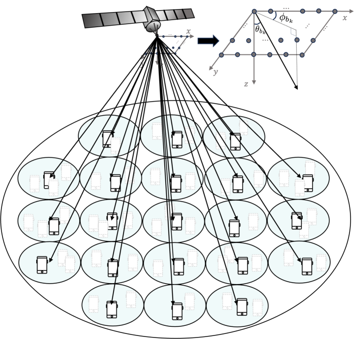
We assume that the ground users are spatially distributed by a homogeneous PPP denoted by with an uniform intensity . Denoting that the whole coverage region of the considered satellite as a disk with radius , follows the Poisson distribution with mean . For convenience, we let the whole coverage region be . Additionally, we also assume that each beam covers a designated region denoted as , and the coverage region of the -th beam is a disk with radius for . Accordingly, the average number of users included in the -th beam’s coverage region is . Our network model is illustrated in Fig. 1.
II-B Channel Model
We describe the large-scale fading, the small-scale fading, and the array steering vector as follows.
Large-scale fading: For user , the large-scale path-loss gain is given by
| (1) |
where and denote the speed of light and the carrier frequency. Also, is the distance from the satellite to user .
| Shadowing Scenario | |||
|---|---|---|---|
| Frequent heavy shadowing | 0.063 | 0.739 | |
| Infrequent light shadowing | 1.29 | 0.158 | 19.4 |
| Average shadowing | 0.835 | 0.126 | 10.1 |
Small-scale fading: We let the small-scale fading drawn from the Shadowed-Rician (SR) distribution. Note that the SR distribution is known to suitably reflect the satellite propagation environments as shown in [27, 18, 28]. For , the fading power is denoted as whose probability density function (pdf) is given by
| (2) |
as presented in [29]. In (2), is a confluent hypergeometric function of the first kind, is the average power of scatter component, is the average power of LoS component and is the Nakagami parameter. For different shadowing scenario, we use the SR fading parameters specified in Table I, as referred in [18, 30].
Array steering vector: Considering the UPA, we define the array steering vector as
denotes the Kronecker product and the is given by
and
| (3) |
Here, and are the inter-antenna spacing and the carrier wavelength, respectively. We adopt the half-wavelength antenna spacing, i.e., . Given that the GEO satellite is geostationarily positioned at the nadir of the center of the coverage region, and are elevation angle and azimuth angle of the user respectively, as depicted Fig. 1
Combining the large-scale fading, the small-scale fading, and the array steering vector, the propagation channel for user is modeled as
| (4) |
where is the large-scale fading defined in (1) and is the small-scale fading defined in (2). Notice that a LoS propagation environment is considered in (4). This is because if a propagation distance significantly exceeds a region of reflection reaching a user, the reflected path length becomes negligible, effectively resulting in LoS channel. We also note that this assumption has been adopted in several prior works such as [6, 22].
II-C Precoding Model
Next, we explain the precoding model. By incorporating the beam pattern of the UPA [31], we divide the coverage area into an uniform grid and place the beam centers at each grid point. For example, the center point of the -th beam is configured as
| (5) |
where and and are elevation angle and azimuth angle of the -th beam, respectively. is a parameter that adjusts the beam spacing. By increasing , the beam spacing becomes narrower, and by decreasing , the beam spacing becomes wider. Specifically, when , each beam is positioned at the first null point of the adjacent beam’s pattern, where each beam covers the region of a disk with radius where is the altitude of the GEO satellite. A detailed analysis of beam spacing and interference levels will be conducted in Section IV. According to this beam construction, the precoding vector for the -th beam, denoted as , is formed as
| (6) |
We clarify that the precoding vectors do not change depending on the CSI of the ground users. Without loss of generality, we denote the coverage region corresponding to the -th beam as , so that , where . Notice that we consider digital precoding, so that multiple payloads are precoded and sent simultaneously.
Subsequently, we describe the user selection. In order to select a user for -th beam, we first extract the users located within and form a candidate set . In , we select the user whose distance to the corresponding beam center is minimum, i.e.,
| (7) |
where is the spatial location of the -th beam on the ground in (5). After selecting a user per beam, the satellite sends the messages through the predefined precoding vectors . Since we only select the users by exploiting the spatial locations, no instantaneous CSI feedback is required in this stage.111 The user selection process may favor only users located in specific spatial regions, especially those located close to the corresponding beam center. To address this, it is possible to design multiple precoder sets, each with beam centers directed towards different spatial locations. Then these sets are used alternatively across time-frequency resources, enabling the satellite to provide ubiquitous coverage. This approach is particularly suitable to the considered UPA since it is very flexible in forming diverse beam patterns. In contrast, a parabolic reflector array requires to physically adjust the reflector, which hinders to form various beams.
Remark 1 (Multi-user diversity with small overheads).
As mentioned earlier, our transmission strategy is closely connected to the multi-user diversity [15, 16]. Similar to our method, [15, 16] also formed multiple fixed-beams and selected a proper user to obtain the multi-user diversity gains. In [15, 16], to select suitable users, all the users compute the individual SINR based on the predefined beams and send the SINR feedback to a transmitter. Then, a transmitter chooses the user that has the maximum SINR. Using such a user selection method in the considered satellite communications, however, is not practical since the feedback amount increases with the total number of users (not the number of beams) in the coverage region. By considering very large number of users in the total coverage region and long link distance between the satellite and the ground users, it induces tremendous overheads. On the contrary to that, in our case, we only exploit the spatial locations of the users, which is slowly varying and easy to obtain. For this reason, it is feasible to select the users without sending extremely large amount of feedback to the satellite. With the assistance of terrestrial networks, it is also possible to completely eliminate the feedback sent to the satellite associated with user selection. Assume that the terrestrial networks can track the spatial locations of all ground users. Since the predetermined beams used at the satellite remain unchanged, their center points also can be known to the terrestrial network. Consequently, suitable user sets can be determined by calculating (7) and then reported to the satellite through the gateway.
Remark 2 (Satellite array model).
In this remark, we compare the parabolic reflector array commonly considered in the previous studies on GEO multibeam satellites, with the phased array, which is the primary focus of this paper. The parabolic reflector array is one of the most classic type of directive antennas. It uses a parabolic-shaped reflector to focus the propagated signals, by which it achieves high beam gain with low complexity and low power consumption. Thanks to this benefit, the parabolic reflector array has been commonly used in multibeam satellite systems [18, 6]. Nonetheless, since its beam steering should rely on physically moving the reflector, the parabolic reflector array has limited flexibility in generating and adjusting multiple beams. For instance, considering a single feed per beam case, number of reflectors are needed to make spot beams [32]. Additionally, the reflector can be bulky and heavy, which is a significant drawback for satellite payloads.
On contrary to that, the phased arrays are composed of a large number of small discrete antenna elements arranged in a certain grid, where each element has its own feed and they are controlled electronically. Because of this feature, the beam steering in the phased array is done by electronically adjusting the phase and amplitude of the signals of each antenna element, allowing rapid and precise beam steering without physically moving the aperture. The phased array was not popular for satellite communications due to high complexity and cost. However, with recent advancements in phased array hardware and their powerful beam steering capabilities, the phased array is increasingly considered a viable and beneficial option. This applies not only to LEO satellite communications [33, 34], but also to GEO satellite communications as demonstrated in several studies [35, 36, 37, 38]. This justifies our consideration.
To make it more understandable, we compare the beam gain functions between the parabolic reflector array and the phased array. In the reflector array, we assume to use the tapered-aperture feed reflector [17, 39, 27]. With the nadir-pointing beam, we denote the associated user whose the distance from beam center to the user is and the azimuth angle is . Then, the beam gain of the parabolic reflector array is approximated as [40, 39]
| (8) |
where and are the first-kind Bessel function of order 1 and 3, respectively. In addition, , where and is the altitude of satellite. is a constant angle associated to the corresponding beam’s 3dB angle. Under the same assumption, the beam gain of the phased array is
| (9) |
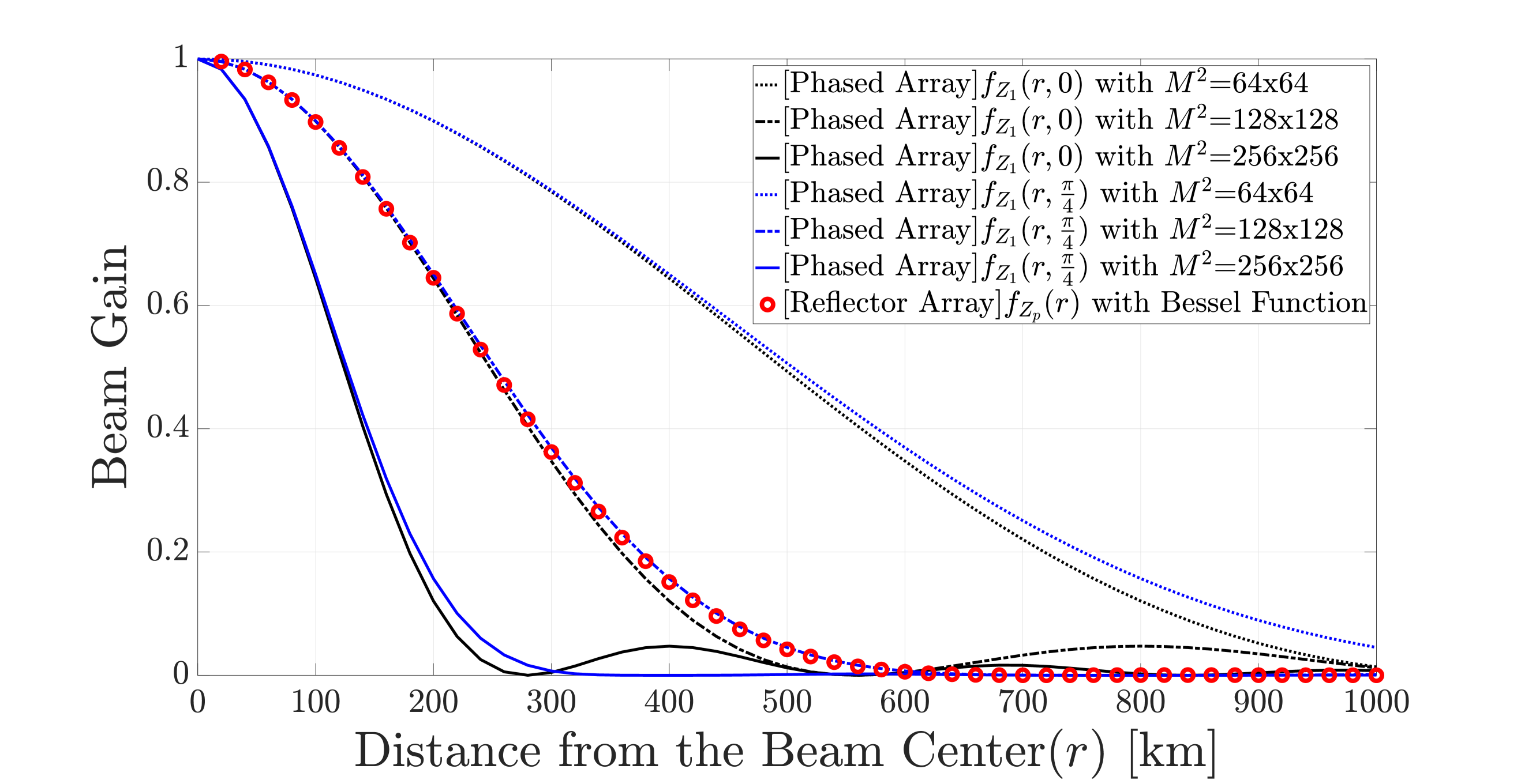
where (a) follows that the inner product of two array response vector is represented as Fejér kernel with in [16] and . The beam gain, which indicates how well the precoding vector aligns with the associated user’s channel, has a value between 0 and 1. The comparison of the beam gain of a reflector array and a phased array with different azimuth angle and is depicted in Fig. 2.
Remark 3 (Rain attenuation).
Rain attenuation is one of the factors affecting satellite communication performance. It typically exhibits spatial correlation over tens of kilometers and changes very slowly [6]. Since our fixed-beam precoding approach selects the user for beam within the coverage region , it is feasible to assume that the candidate users in experience identical rain attenuation. For this reason, rain attenuation remains constant and does not influence the asymptotic scaling analysis. This assumption aligns with the approach taken in [18].
III A Single Beam Case
In this section, we first focus on a single beam case, i.e., and analyze the rate performance. We extend this setup to a multiple beam case in the next section.
III-A Achievable Rate Analysis
The satellite operates a single beam and selects the user based on the distance from the beam. Here, the beam is a nadir-pointing fixed-beam. Without loss of generality, the selected user is assigned the index . The reason we analyze the nadir-pointing fixed-beam and the corresponding user is that it causes the largest variation in beam gain for the same distance . Then, the received SNR for user is given by
| (10) |
where and denote the transmit and receiver antenna gains. Additionally, where is the transmit power of the satellite, is Boltzmann constant and is bandwidth, respectively. We also note that the fading power is drawn from the PDF (2). is a beam gain function defined as (9) with the nadir-pointing beam, i.e., . By leveraging this, we derive the achievable rate of the user in the following theorem.
| (11) |
Theorem 1.
In a single beam case, we define the achievable ergodic rate as
| (12) |
where the expectation is regarding the randomness associated with the fading power and the spatial locations of the ground users. Then is obtained as in (11).
Proof.
Assuming a random variable where , we have
where (a) follows [41]
| (13) |
and (b) follows the moment generating function (MGF) of given by [29]
| (14) |
Now we obtain the PDF of and . Recalling that , we get the conditional PDF of as
| (15) |
The proof of (15) is straightforward in proof of Lemma 2, especially (27). Here, is independent to which is calculated in isolation by . Then, by putting , this completes the proof. ∎
| Parameter | Value |
|---|---|
| Satellite height | km |
| Link frequency band | GHz (Ka) |
| Beam bandwidth | MHz |
| Noise temperature | K |
| Boltzmann constant | |
| User antenna gain | 41.7 dBi |
| Satellite antenna gain | 52 dBi |
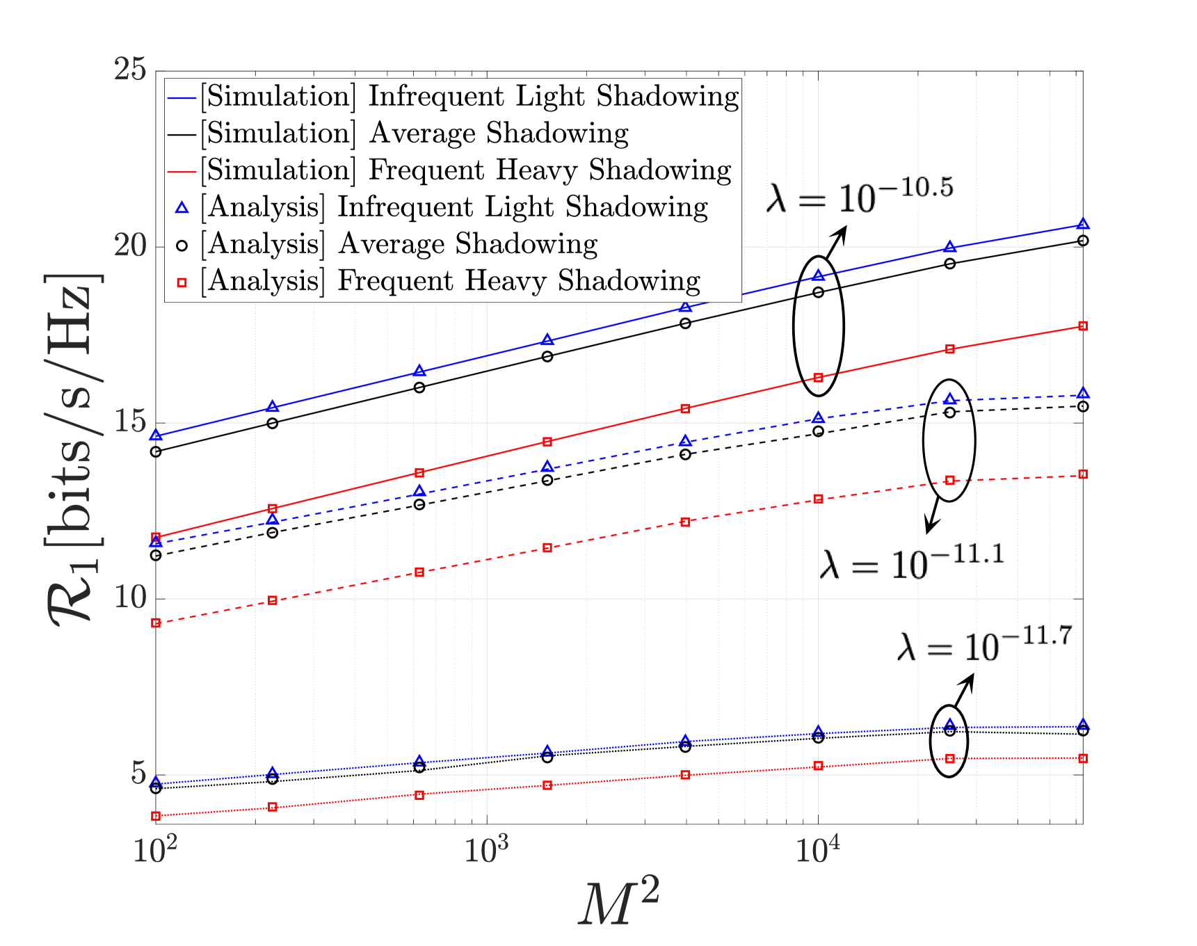
Now we validate our analysis by comparing to the simulation result. The SR fading parameters and the used simulation parameters are are in listed in Table I and Table II, respectively. We also clarify that Table II is referred from [6, 18, 30]. Fig. 3 shows for different as increasing with whose beam width is typically used in GEO satellite. The result indicates that the analytical results are well matched to the numerical simulations. One interesting observation of Fig. 3 is that the scaling behavior of the ergodic rate with is different depending on . That is to say, when is sufficiently large, increases with , while is relatively small, the growth of rather slows down. In particular, when , increasing does not necessarily increase ; but rather decreases as increases. The rationale behind this is as follows. Recall that we employ the fixed-beam precoding approach, in which the precoding vectors are not adjusted depending on CSI. As a result, it is possible that the selected user is not located at the exact beam center point, causing a beam mismatch. As illustrated in Fig. 2, this beam mismatch results in a reduction of the beam gain. Now, let’s assume that increases asymptotically. If the user is exactly at the beam center, the SNR also increases asymptotically thanks to the boosted array gain. On the contrary, if the beam mismatch occurs in the fixed-beam precoding approach, increasing leads to narrower beam width; thereby the selected user tends to be located outside of the main beam width. For instance, , the main-lobe beam width also goes to and this makes the corresponding beam gain for constant . To prevent this, should scale up with . In summary, to ensure non-vanishing ergodic rate in the multibeam satellite communication with massive MIMO where is very large, should increase with at a certain scaling parameter, i.e., (here, implies ). Identifying the scaling parameter is crucial in understanding and designing the considered satellite communication system. In the next subsection, we reveal this scaling law.
III-B Asymptotical Scaling Law Analysis
We analyze the scaling behavior as and increase. The following theorem is a main result of this subsection.
Theorem 2.
Let for any and with arbitrarily small . Then, we have asymptotic upper and lower bounds of as
| (16) |
Proof.
Please see Appendix A. ∎
From the upper and lower bounds in Theorem 2, we get . This implies that, if , then the achievable ergodic rate achieves a positive gain as . Otherwise goes to , i.e., it is infeasible to provide stable ergodic rate in the satellite communication with massive MIMO. Since the number of the antennas on the UPA is , corresponds to the square root of the number of antennas. This implies that the ground user density should scale with at least the square root of the number of UPA antennas. If , i.e., the user density scales with the same rate as the number of antennas, the achievable rate scales with , which indicates the ideal ergodic rate when perfect CSI is given to the satellite. In the following corollary, we further reveal this.
Corollary 1.
For with for with arbitrarily small , we have
| (17) |
Proof.
See Appendix B. ∎
In (17), the denominator corresponds to the ideal ergodic rate by matching the beam center to the corresponding user’s location, i.e., . To this end, the selected user needs to send the CSI feedback to the satellite, then the satellite aligns its precoding vector to the received CSI. Since the fixed-beam precoding approach does not adjust the precoding vector to the ground user, the ideal ergodic rate is consistently larger than the achievable ergodic rate . For this reason, the ratio in (17) is interpreted as the extent of performance degradation caused by not sending the CSI feedback. As shown in Corollary 1, the fixed-beam precoding approach achieves the fraction of of the ideal rate when . From this, we find that is necessary for achieving non-vanishing ergodic rate as observed in Theorem 2. If , i.e., , then the fixed-beam precoding approach asymptotically achieves the ideal ergodic rate, implying that no CSI is needed to achieve the optimal rate.
IV A Multiple-Beam Case
In this section, we extend our analysis by incorporating a multiple beam case. We consider that the satellite forms number of beams to serve spot regions. For the -th spot region , we select a user according to (7) and use the precoder as described in (6). Without loss of generality, we denote the user index selected for beam as and beam is the nadir-pointing located at the center of the coverage region. Similar to the single beam case, we first characterize the achievable ergodic rate as a function of the system parameters and study the scaling laws.
IV-A Achievable Rate Analysis
In the multibeam scenario, it is of importance to properly account for the amount of inter-beam interference. To this end, we denote as the beam gain that user receives from the -th fixed-beam. Accordingly, indicates the amount of interfering beam gain from the -th beam with . With this, the signal-to-interference-plus-noise-ratio (SINR) of user is given by
| (18) |
where the allocated transmit power is divided by as , is the large-scale fading of user as in (1) and is the fading power drawn from the PDF (2). The sum ergodic rate of the multiple beam case is defined by
| (19) |
Now we analyze the achievable ergodic rate in the multibeam case. In this analysis, we focus on user ’s ergodic rate as a representative case.
Theorem 3.
In the multibeam case, we define the ergodic rate of user as
where the expectation is about the randomness associated with the fading power, spatial locations of ground users. Then, the is obtained in (20).
| (20) |
Proof.
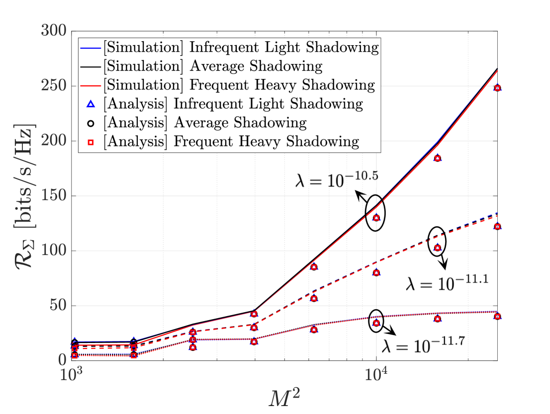
The rationale for choosing user as a representative case is as follows: First, since spot beam , which is a nadir-pointing beam as shown in Fig. 1, is surrounded by other beams, user is most susceptible to inter-beam interference, thus representing the lower bound of network performance. Second, if extending to large networks with multiple satellites that each cover their own area, users at the edge of each coverage may experience inter-satellite interference. Although we analyze a single satellite here, it is reasonable to investigate the performance of user using the wrap-around technique to understand the overall system performance. This is observed in Fig. 4, which compares the simulation and analysis of the ergodic sum rate for different and SR parameters. The parameters used in Fig. 4 are listed in Table I and Table II. The analysis results are obtained by multiplying the analytical result of in (20) by the total number of beams . Consistent with our intuition, the analytical sum rate using serves as a lower bound for the obtained simulation sum rate.
Understanding the asymptotic behavior between the user density , the number of beams , and the number of antennas is crucial for gaining design insights into the multibeam satellite communication system. However, analyzing the multiple beam case is more complicated compared to the single beam case due to the challenge of capturing inter-beam interference. In the next subsection, we clarify the difficulty and put forth our idea to resolve this.
IV-B Asymptotical Scaling Law Analysis
In this subsection, we study the scaling laws between , , and . A key hindrance of the analysis is characterizing the amount of inter-beam interference in a tractable manner. The amount of inter-beam interference is mainly determined by the inter-beam spacing and the beam width. To capture this, we recall that the inter-beam spacing is controlled by the parameter as outlined in the beam configuration (5), wherein we examine within the range in the analysis. It is clear increasing narrows the inter-beam spacing, leading to higher inter-beam interference. However, this allows for more beam multiplexing gains are attained by using more beams. Conversely, decreasing alleviates the inter-beam interference, while limiting the beam multiplexing gains.
As a key ingredient of the scaling law analysis in the multiple beam case, we comprehend the inter-beam interference experienced by user from another fixed-beam in relation to . Since the number of spot beams that can be packed in is scaled with , we assume where is obtained by solving a circle packing problem for given inter-beam spacing. Obtaining for given specific and is interesting yet beyond the scope of our paper. In an asymptotic regime of our interest, it is possible to choose because the inter-beam spacing becomes sufficiently small as increases, so that number of beams can be packed within . We characterize the inter-bream in the following lemma.
Lemma 1.
For such that , we have
| (22) |
where .
Proof.
Please see Appendix C. ∎
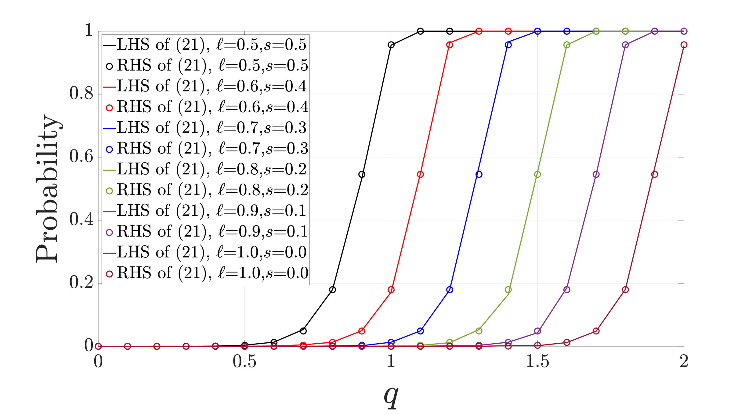
Fig. 5 shows the probability that the interference from a adjacent beam (where and in (5)) is below a certain level, i.e., . As shown in Fig. 5, the left-hand-side (LHS) of Lemma 1 is followed by the right-hand-side (RHS) of Lemma 1. The results validates the result of Lemma 1.
To explore Lemma 1 deeply, we introduce an auxiliary variable such that . If increases, then decreases. In this case, the beam spacing becomes narrow, which leads to increase interference level. Nevertheless, to ensure the interference remains to be below certain level, more user density is required to compensate for the reduced beam spacing according to , which is denoted as . Conversely, if decreases then increases, which means the beam spacing widens, allowing for less interference. Because the numerator of is equivalent to of the single beam case which achieves a fraction of the optimal performance a single beam when . Therefore, from the perspective of beam matching for each user, achieving alignment equivalent to that of a single beam is possible in Lemma 1 under the condition . By using this, we derive following theorem.
Theorem 4.
For with and such that , and , the expected rate of user with multiple-beam is given by
| (23) |
as .
Proof.
Please see Appendix D. ∎
Now we elucidate Theorem 4. To achieve non-vanishing performance in multiple fixed-beam, larger density such that is required, which contrasts to the single beam case that requires . In other words, in multi-beam scenarios, it is necessary to boost the user density by to compensate the impact of interference. We extend Theorem 4 to the sum rate in the following corollary.
Corollary 2.
For with such that , and , we have
| (24) |
Proof.
Please refer to Appendix E. ∎
The denominator denotes the ideal ergodic rate for user by perfectly eliminating the interference, provided that precoding is used with perfect CSI. To be specific, implies that the considered fixed-beam precoding method achieves such a fraction of the optimal performance, while for implies the multiplexing gain. In this point of view, when focusing on single beam with interference, it requires an additional user density of compared to a single beam without interference. However, with the additional required , a multiplexing gain of can be achieved. Moreover, when the user density scales with the number of antennas, i.e., q=2, the asymptotic optimal sum rate can be achieved regardless of . On the other hand, when the number of beam , i.e., , the result of Corollary 2 is reduced to , which matches well with the result of Corollary 1 for a single beam case. Furthermore, the sum rate exhibits different slopes with respect to as increases. This aligns with the results with Fig. 4.
Remark 4 (Extension to multicast scenario).
In a certain satellite communication scenario such as DVB-S2X, serving multiple users per beam, i.e., multicast, is desirable. If a satellite serves users per beam, the considered fixed-beam precoding approach can be extended to a scenario that the satellite communicates with the nearest users in each beam with a PPP with density . Assuming that the users in each beam are indexed in order of proximity as , the rate achievable by the beam is determined by user . This is because minimum of SNRs for users per beam should be carried on for multicasting. Thus, the probability of the distance between user and the corresponding beam center, denoted by , is obtained by
| (25) |
It is interesting to extend our analytical framework by incorporating (25) in Lemma 2.
V Conclusion
In this paper, we have considered a fixed-beam precoding approach for massive MIMO multibeam satellite communication systems combined with a location based user-selection strategy. Upon this, we have provided a performance analysis, that sheds light on the asymptotical interplay between the density of ground users, the number of beams and the number of antennas. Our major findings are that when the user density is scaling at the identical rate with the number of antennas, then the fixed-beam precoding is able to provide enough beam gain even without CSI while the beam mismatch becomes negligible. In the multiple beam case, we have found that the scale of the interference is adjusted by the beam spacing, while providing the probability of the interference scale as a function of user density. Moreover, the the fixed-beam precoding, when user density scales with the number of antennas, achieves the asymptotic optimal sum rate regardless of the beam spacing. The current analysis is based on a single user per beam approach, and extending this analysis to a multicast scenario remains future work.
Appendix A Proof of Theorem 2
Before proving the Theorem 2, we introduces the useful lemma to use the subsequent proofs.
Lemma 2.
We denote the homogeneous PPP where follows the PPP with average number . Then, the probability that the distance of the nearest user from the nadir-pointing beam is in range between and is given by
| (26) |
where .
Proof.
The probability of which is the distance from the beam to nearest user within the range between and where is given by
For the case , the probability about equals to 0. Then, we have
| (27) |
where is the independent PPP for excluding the region of . This is the end of proof. ∎
To prove of Theorem 2, we investigate defined as
| (28) |
where . To do this, we analyze the event conditioned on two case for : when and when .
Case 1 (): The event is given by
which is equal to
The sufficient conditions for for small are given by
| (29) |
and
| (30) |
Using the fact that for small , the sufficient conditions for are
which can be reformulated as
Also, by using the fact for , the sufficient condition for (30) is denoted as
which is reformulated as
Thus, the sufficient condition for the event is given by
| (31) |
where is the constant for the given . Substituting the , the range of satisfying (31) is written as
| (32) |
Thus, the probability of is lower bounded with the probability of (32) by using Lemma 2 as
| (33) | |||
where (a) holds for the region .
Case 2 (): We obtain the and from (II-B) when . Then, the event is given by
| (34) |
We can find the sufficient conditions of (34) as
and
From the sufficient condition, we obtain the bound of using the same approach when as
| (35) |
with the , the range of satisfying (35)
Thus, the probability of the event when is lower bounded as
where (a) holds when . We note that is always satisfied with .
From these results, we obtain lower and upper bounds on where ranges within (32) as
| (36) |
where and are the lower and upper bound of , respectively. We have to note that as for . Here, by setting , the lower bound is derived as
By setting , we obtain the upper bound as
where (a) is from the fact that by using (33), we know that for . Then, we have
We can modify this result into
| (37) |
where is independent to the distance . From the fact where and , the lower bound of for with for is obtained by
| (38) |
where (a) holds from (37) by letting , (b) is from properties of log, (c) is the definition of expectation where is in (2) and (d) holds when is the constant independent to . The upper bound is obtained by similar approach such as
| (39) |
where with for . This proof refers to [16]. Then, the derived lower and upper bound of is given by
| (40) |
As , we conclude the proof.
Appendix B Proof of Corollary 1
Appendix C Proof of Lemma 1
For , the event is equivalent to
| (43) |
where . We have the two sufficient conditions for (43) as
| (44) |
and
| (45) |
Here, focusing on (44), we have
| (46) |
By using , we have
| (47) |
From the fact that for , we have
| (48) |
and with and
| (49) |
Relaxing in terms of absolute value, we have
where are coordinates of user in the nadir-pointing beam’s coverage and is always located at the point outside the nadir-pointing beam’s coverage. (b) comes from . Then, we have
| (50) |
and for with sufficiently large
| (51) |
The procedure of sufficient condition (45) is almost similar with (44) and given by
| (52) |
which is corresponding to (49). And, the result is equal to (51). Therefore, the probability of (43) is given by
| (53) |
where (a) is and (b) is using Lemma 2. This is the end of proof.
Appendix D Proof of Theorem 4
The lower bound of is given by
| (54) |
where (a) comes from with . (b) holds by the Jensen’s inequality, (c) is Lemma 1 for and such that , (d) holds for sufficiently large , and (e) is straightforward referring to (38). The upper bound is obtained with similar approach as
| (55) |
where (a) comes from with . (b) holds by ignoring the interference, (c) is also from (39). The derivation is straightforward referring to (54). Then, the bound of is given by
| (56) |
where is the constant independent to . For with small positive , we conclude the proof.
Appendix E Proof of Corollary 2
References
- [1] M. A. Vazquez, A. Perez-Neira, D. Christopoulos, S. Chatzinotas, B. Ottersten, P.-D. Arapoglou, A. Ginesi, and G. Taricco, “Precoding in multibeam satellite communications: Present and Future Challenges,” IEEE Wireless Commun., vol. 23, no. 6, pp. 88–95, 2016.
- [2] A. I. Perez-Neira, M. A. Vazquez, M. B. Shankar, S. Maleki, and S. Chatzinotas, “Signal processing for high-throughput satellites: Challenges in new interference-limited scenarios,” IEEE Signal Process. Mag., vol. 36, no. 4, pp. 112–131, 2019.
- [3] M. Khammassi, A. Kammoun, and M.-S. Alouini, “Precoding for high-throughput satellite communication systems: A survey,” IEEE Commun. Surveys & Tutorials, vol. 26, no. 1, pp. 80–118, 2024.
- [4] P.-D. Arapoglou, K. Liolis, M. Bertinelli, A. Panagopoulos, P. Cottis, and R. De Gaudenzi, “MIMO over satellite: A review,” IEEE Commun. Surveys & Tutorials, vol. 13, no. 1, pp. 27–51, 2011.
- [5] S. Chatzinotas, G. Zheng, and B. Ottersten, “Energy-efficient MMSE beamforming and power allocation in multibeam satellite systems,” in Proc. of Asilomar Conf. on Signal, Systems and Computers, 2011, pp. 1081–1085.
- [6] G. Zheng, S. Chatzinotas, and B. Ottersten, “Generic optimization of linear precoding in multibeam satellite systems,” IEEE Trans. Wireless Commun., vol. 11, no. 6, pp. 2308–2320, 2012.
- [7] D. Christopoulos, S. Chatzinotas, and B. Ottersten, “Multicast multigroup precoding and user scheduling for frame-based satellite communications,” IEEE Trans. Wireless Commun., vol. 14, no. 9, pp. 4695–4707, 2015.
- [8] V. Joroughi, M. A. Vázquez, and A. I. Pérez-Neira, “Generalized multicast multibeam precoding for satellite communications,” IEEE Trans. Wireless Commun., vol. 16, no. 2, pp. 952–966, 2017.
- [9] M. A. Vazquez, M. R. B. Shankar, C. I. Kourogiorgas, P.-D. Arapoglou, V. Icolari, S. Chatzinotas, A. D. Panagopoulos, and A. I. Perez-Neira, “Precoding, scheduling, and link adaptation in mobile interactive multibeam satellite systems,” IEEE J. Sel. Areas Commun., vol. 36, no. 5, pp. 971–980, 2018.
- [10] R. T. Schwarz, T. Delamotte, K.-U. Storek, and A. Knopp, “MIMO applications for multibeam satellites,” IEEE Trans. Broadcasting, vol. 65, no. 4, pp. 664–681, 2019.
- [11] V. Joroughi, M. A. Vazquez, and A. I. Perez-Neira, “Precoding in multigateway multibeam satellite systems,” IEEE Trans. Wireless Commun., vol. 15, no. 7, pp. 4944–4956, 2016.
- [12] J. Park, N. Lee, J. G. Andrews, and R. W. Heath, “On the optimal feedback rate in interference-limited multi-antenna cellular systems,” IEEE Trans. Wireless Commun., vol. 15, no. 8, pp. 5748–5762, 2016.
- [13] N. Jindal, “MIMO broadcast channels with finite-rate feedback,” IEEE Trans. Inf. Theory, vol. 52, no. 11, pp. 5045–5060, 2006.
- [14] I. Ahmad, K. D. Nguyen, N. Letzepis, G. Lechner, and V. Joroughi, “Zero-forcing precoding with partial CSI in multibeam high throughput satellite systems,” IEEE Trans. Veh. Technol., vol. 70, no. 2, pp. 1410–1420, 2021.
- [15] M. Sharif and B. Hassibi, “On the capacity of MIMO broadcast channels with partial side information,” IEEE Trans. Inf. Theory, vol. 51, no. 2, pp. 506–522, 2005.
- [16] G. Lee, Y. Sung, and J. Seo, “Randomly-directional beamforming in millimeter-wave multiuser MISO downlink,” IEEE Trans. Wireless Commun., vol. 15, no. 2, pp. 1086–1100, 2016.
- [17] N. Zorba, M. Realp, and A. I. Perez-Neira, “An improved partial CSIT random beamforming for multibeam satellite systems,” in Proc. Int. Workshop on Signal Process. for Space Commun., 2008, pp. 1–8.
- [18] D.-H. Na, K.-H. Park, Y.-C. Ko, and M.-S. Alouini, “Performance analysis of satellite communication systems with randomly located ground users,” IEEE Trans. Wireless Commun., vol. 21, no. 1, pp. 621–634, 2022.
- [19] E. G. Larsson, O. Edfors, F. Tufvesson, and T. L. Marzetta, “Massive MIMO for next generation wireless systems,” IEEE Commun. Mag, vol. 52, no. 2, pp. 186–195, 2014.
- [20] F. Rusek, D. Persson, B. K. Lau, E. G. Larsson, T. L. Marzetta, O. Edfors, and F. Tufvesson, “Scaling up MIMO: Opportunities and challenges with very large arrays,” IEEE Signal Process. Mag., vol. 30, no. 1, pp. 40–60, 2013.
- [21] H. Q. Ngo, E. G. Larsson, and T. L. Marzetta, “Aspects of favorable propagation in massive MIMO,” in European Signal Process. Conf. (EUSIPCO), 2014, pp. 76–80.
- [22] P. Angeletti and R. De Gaudenzi, “A pragmatic approach to massive MIMO for broadband communication satellites,” IEEE Access, vol. 8, pp. 132 212–132 236, 2020.
- [23] J. Park, J. Choi, and N. Lee, “A tractable approach to coverage analysis in downlink satellite networks,” IEEE Trans. Wireless Commun., vol. 22, no. 2, pp. 793–807, 2023.
- [24] D. Kim, J. Park, and N. Lee, “Coverage analysis of dynamic coordinated beamforming for LEO satellite downlink networks,” IEEE Trans. Wireless Commun., pp. 1–1, 2024.
- [25] N. Okati, T. Riihonen, D. Korpi, I. Angervuori, and R. Wichman, “Downlink coverage and rate analysis of low earth orbit satellite constellations using stochastic geometry,” IEEE Trans. Commun., vol. 68, no. 8, pp. 5120–5134, 2020.
- [26] N. Okati and T. Riihonen, “Nonhomogeneous stochastic geometry analysis of massive LEO communication constellations,” IEEE Trans. Commun., vol. 70, no. 3, pp. 1848–1860, 2022.
- [27] A. Talgat, M. A. Kishk, and M.-S. Alouini, “Stochastic geometry-based uplink performance analysis of IoT over LEO satellite communication,” IEEE Trans. Aerosp. Electron. Syst, pp. 1–15, 2024.
- [28] M. Sellathurai, S. Vuppala, and T. Ratnarajah, “User selection for multi-beam satellite channels: A stochastic geometry perspective,” in Proc. of Asilomar Conf. on Signal, Systems and Computers, 2016, pp. 487–491.
- [29] A. Abdi, W. Lau, M.-S. Alouini, and M. Kaveh, “A new simple model for land mobile satellite channels: first- and second-order statistics,” IEEE Trans. Wireless Commun., vol. 2, no. 3, pp. 519–528, 2003.
- [30] J. Wang, L. Zhou, K. Yang, X. Wang, and Y. Liu, “Multicast precoding for multigateway multibeam satellite systems with feeder link interference,” IEEE Trans. Wireless Commun., vol. 18, no. 3, pp. 1637–1650, 2019.
- [31] H. L. Van Trees, Optimum array processing: Part IV of detection, estimation, and modulation theory. John Wiley & Sons, 2002.
- [32] M. Schneider, C. Hartwanger, and H. Wolf, “Antennas for multiple spot beam satellites,” CEAS Space Journal, vol. 2, no. 1, pp. 59–66, 2011.
- [33] D. Kim, S. Cho, W. Shin, J. Park, and D. K. Kim, “Distributed precoding for satellite-terrestrial integrated networks without sharing CSIT: A rate-splitting approach,” ArXiv, 2024. [Online]. Available: https://arxiv.org/abs/2309.06325
- [34] L. You, K.-X. Li, J. Wang, X. Gao, X.-G. Xia, and B. Ottersten, “Massive MIMO transmission for LEO satellite communications,” IEEE J. Sel. Areas Commun., vol. 38, no. 8, pp. 1851–1865, 2020.
- [35] B. Tian, Y. Li, M. Cai, H. Liu, and Y. Luo, “Design of Ka-band active phased-array antenna for GEO communication satellite payloads,” in Proc. Int. Applied Computational Electromagnetics Society Symposium (ACES), 2017, pp. 1–2.
- [36] J. B. L. Rao, R. Mital, D. P. Patel, M. G. Parent, and G. Tavik, “Low-cost multibeam phased array antenna for communications with GEO satellites,” IEEE Aerospace and Electronic Systems Mag., vol. 28, no. 6, pp. 32–37, 2013.
- [37] J. Warshowsky, C. Kulisan, and D. Vail, “20 GHz phased array antenna for GEO satellite communications,” in Proc. IEEE Military Commun. Conf. (MILCOM), vol. 2, 2000, pp. 1187–1191 vol.2.
- [38] L. Yu, J. Wan, K. Zhang, F. Teng, L. Lei, and Y. Liu, “Spaceborne multibeam phased array antennas for satellite communications,” IEEE Aerospace and Electronic Systems Mag., vol. 38, no. 3, pp. 28–47, 2023.
- [39] J. Arnau, D. Christopoulos, S. Chatzinotas, C. Mosquera, and B. Ottersten, “Performance of the multibeam satellite return link with correlated rain attenuation,” IEEE Trans. Wireless Commun., vol. 13, no. 11, pp. 6286–6299, 2014.
- [40] C. Caini, G. Corazza, G. Falciasecca, M. Ruggieri, and F. Vatalaro, “A spectrum- and power-efficient ehf mobile satellite system to be integrated with terrestrial cellular systems,” IEEE J. Sel. Areas Commun., vol. 10, no. 8, pp. 1315–1325, 1992.
- [41] K. A. Hamdi, “A useful lemma for capacity analysis of fading interference channels,” IEEE Trans. Commun., vol. 58, no. 2, pp. 411–416, 2010.