Gaussian Processes for extrapolative inference:
A powerful tool for addressing model-dependency and uncertainty
Inference at the data’s edge: Gaussian processes for modeling and inference under model-dependency, poor overlap, and extrapolation ††thanks: Authorship order alphabetical for the first two authors; Hazlett is senior co-author. All authors contributed equally. We thank members of the Practical Causal Inference lab’s learning group for their insightful comments and feedback.
Abstract
The Gaussian Process (GP) is a highly flexible non-linear regression approach that provides a principled approach to handling our uncertainty over predicted (counterfactual) values. It does so by computing a posterior distribution over predicted point as a function of a chosen model space and the observed data, in contrast to conventional approaches that effectively compute uncertainty estimates conditionally on placing full faith in a fitted model. This is especially valuable under conditions of extrapolation or weak overlap, where model dependency poses a severe threat. We first offer an accessible explanation of GPs, and provide an implementation suitable to social science inference problems. In doing so we reduce the number of user-chosen hyperparameters from three to zero. We then illustrate the settings in which GPs can be most valuable: those where conventional approaches have poor properties due to model-dependency/extrapolation in data-sparse regions. Specifically, we apply it to (i) comparisons in which treated and control groups have poor covariate overlap; (ii) interrupted time-series designs, where models are fitted prior to an event by extrapolated after it; and (iii) regression discontinuity, which depends on model estimates taken at or just beyond the edge of their supporting data.
Keywords: causal inference, gaussian process regression, regression discontinuity, interrupted time-series
1 Introduction
When models are fitted on an observed dataset and extended to areas with few observations—or even past the edge of the data—the result will be highly dependent on both the choice of model and the particular data used. Further, conventional modeling approaches rely on choosing a fitted model, then estimating model uncertainty conditional on that model, despite our knowledge that either a different choice of specification or slight alterations to the training data could have altered that model. Thus, uncertainty estimates typically no longer reflect model uncertainty. This can have, as we illustrate, disastrous consequences for uncertainty estimates and inferences we make under approaches that rely on models that go near, to, or beyond the edge of the data. In a seminal paper on this theme King and Zeng, (2006) term these challenges and the risks these pose as the “dangers of extreme counterfactuals”.
This problem is not mitigated—and can be exacerbated—by using more flexible models. For example, if the outcome is fitted by a cubic polynomial of a predictor , then even if the true model is cubic, the fitted model can fluctuate wildly near and beyond the edges of the data. The fact that the underlying model may not be correct only exacerbates this. More generally, in parametric models (e.g. a linear model of the form , for features given by ), the model standard errors will appear to expand as we move away from the data. However, this is only because the estimated variance of will have the form ). While this grows with the amplitude of , it does not respect any information about where the data are dense or sparse. Another interesting example is kernel regularized least squares (KRLS, Hainmueller and Hazlett, 2014), which has the feature that, as we move away from the training data, the estimates of return towards . This is not unreasonable, but unfortunately the uncertainty estimates also become smaller as we move away from the data, because the model is increasingly certain to move towards the overall in these regions. By contrast, intuition suggests that our uncertainty estimates would expand as we move away from the support of the data, as we should be less certain about predicted values where we have less data. These behaviors can be catastrophic in settings where the point and uncertainty estimates depend on model behavior at or near the edge of their support data. As we show below, causal inference problems with poor covariate overlap, interrupted time-series, and regression discontinuity provide a few examples of such circumstances.
In this paper, we explore the use of Gaussian Processes (GPs) as a natural, principled solution to quantifying prediction/counterfactual uncertainty when faced with this danger. GPs have emerged as versatile and powerful tools in various scientific domains. However, they remain relatively underutilized in the realm of social sciences, perhaps due to the difficulty of understanding how they work and software implementations ill-suited for social science applications. To remedy this, we offer an accessible explanation of how GPs work, which requires only a rudimentary background in probability to understand. We also develop a simple and powerful GP implementation that better fits the needs of social scientists. In particular, it reduces the number of hyperparameters that must be chosen or tuned manually from three in most implementations down to zero in ours, without a loss in performance. It also rescales some of the values involved to correspond to values familiar to researchers, such as the .
We then illustrate the potential value of GPs in three settings where investigators need to make inferences near, at, or beyond the edge of the data. First, we consider a common setting where treated and control units that have poor covariate overlap. In this case, we show how a GP (fitted to the treated and controls separately, as for imputation/g-computation/T-learner) correctly accounts for the added uncertainty for the outcome under treatment (control) moving into areas where there were fewer treated (control) units. As a result, pointwise and conditional ATE/ATT/ATC estimates show correct coverage when estimated this way, but catastrophic coverage when using a fixed parametric model (e.g. OLS) or BART.
Second, we briefly demonstrated ways in which GP can be applied to interrupted time-series (ITS), in which the investigator must carry a predictive model for trained on a pre-treatment time-series into the post-treatment era for comparison. The GP is again useful in this setting for its ability to incorporate additional uncertainty we should have as we move away from the training data. Here we face an additional complication that the model space (choice of kernel) becomes paramount, encoding what the investigator is or is not willing to assume about how “extreme” the extrapolation might be.
Third, in regressions discontinuity (RD), the task is to model units from below the cutoff all the way up until the value of the cutoff. The ultimate effect estimate depends on point and uncertainty estimates learned right up to (and possibly very slightly beyond) the edge of the data that support them. Such models would ideally show additional uncertainty as they “run out of data”. GP does this naturally and we show that the results are similar to approaches such as rdrobust (Calonico et al., 2015) while providing slightly better coverage rates, with similar or slightly smaller intervals. We also explore how in some RD settings, “causal assumptions” (from outside the data) can be integrated into the GP procedures rather than relying on data to guide bandwidth selection or data trimming, which may lead to including points far from the cutoff.
2 The GP framework
We now describe the GP framework. While suitable technical introductions are available (see e.g. Rasmussen et al., 2006), our hope is to offer a step-wise and accessible explanation for social scientists not familiar with similar approaches. We do so through the following steps:
A distributional outcome.
The first requirement is to imagine that the outcome variable, , across the observations ( is itself drawn from a multivariate normal distribution, i.e. . That is, we recognize each observation as draws from a distribution that has certain mean and covariance properties. We defer for the moment how and will be determined.
Smoothness, covariance, and functional form.
The second step is to consider a special role for information about covariance between the values of any pair of observations, and more broadly for any proposed pair of points. To start, for two observations and , make the supposition that and should be more similar to each other if and are more similar. In other words, there are many vectors we could have drawn, and many possible shapes for the function , but we can expect that in cases where two observations have similar covariates, they will have similar outcomes. Thus, across the vectors we could have drawn, we can rely on to be high when is nearer to .
More formally, we choose a kernel function that governs the relationship between covariance of with and the distance between and . We write . This can be given a particular form, such as (the Gaussian kernel) whereby observations and will have maximal covariance () when , but the covariance drops towards zero as the Euclidean distance increases between and . However, other kernel functions can be applied to various purposes we discuss below.111The name “Gaussian process” refers to the (Normal) distributional assumption, not the choice of kernel function. Consider the kernel matrix , containing all the pairwise kernel evaluations, i.e. . As this describes the full variance-covariance matrix of the vector , we now have the model
noting that this formulation would allow us to add any additional observation and compute its covariance relative to all others.
In practice, it will be necessary to allow for a role of noise, such that there is additional variance in the values of the observations, changing our model to:
We simplify this by proposing to demean , and to rescale it to have variance 1. We then use (the zero vector) and , arriving at222The assumption of is not a strong one claiming the conditional expectation function is everywhere ; it is an assumption about what we can expect absent any data. The reasoned beliefs we have about the conditional expectation of given (the mode of our posterior belief) given the data will emerge below.
As the overall variance of is now 1, has the additional interpretive value of being the “fraction of not explained by ”, i.e. one minus the we would get if used the conditional expectation function to predict each . We will discuss how (and any parameters of the kernel function) are chosen below.
Conditioning on the data.
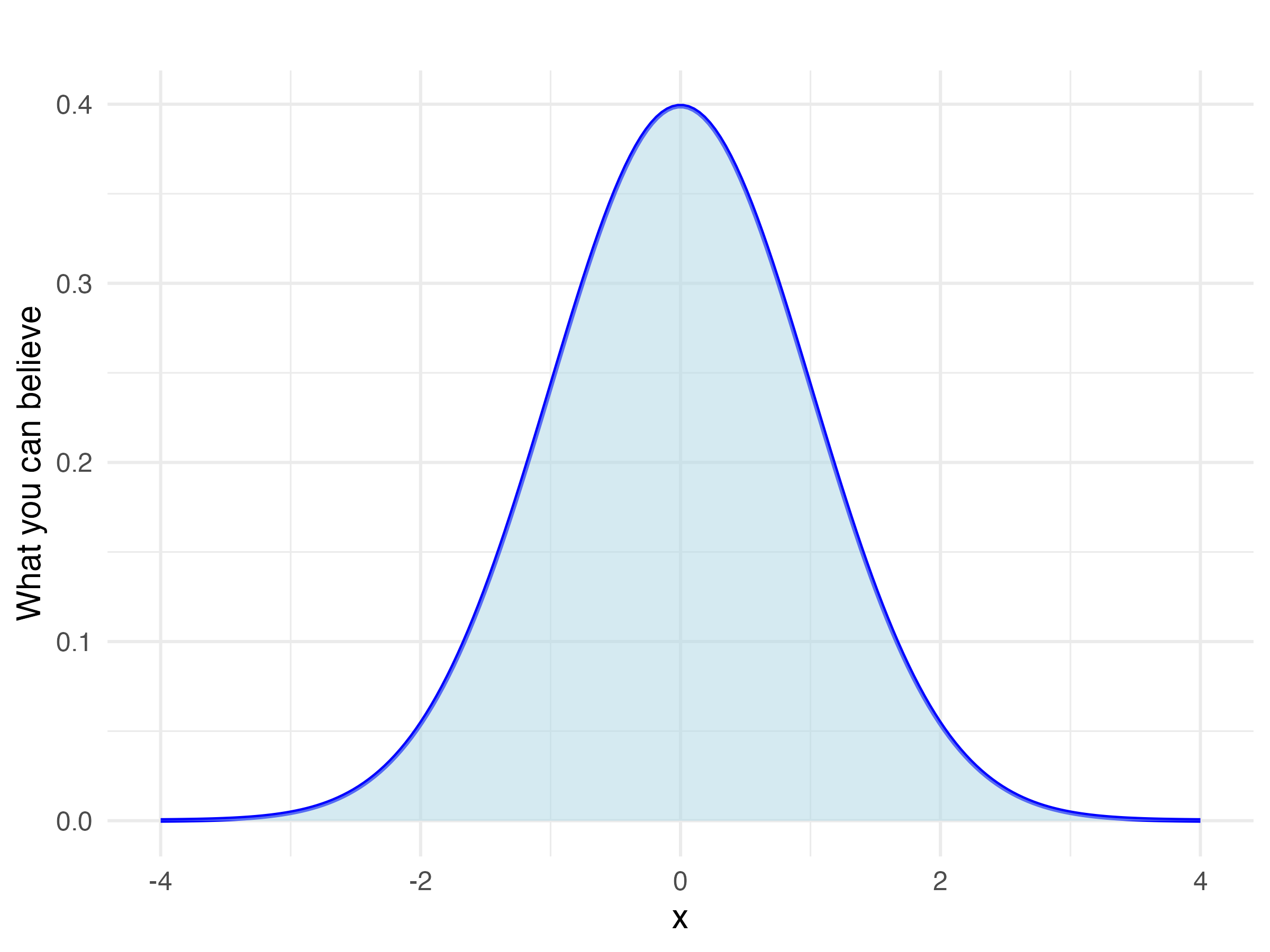
Consider what it means to observe and at some values, for our beliefs about the distribution of at other locations in the covariate space, given just this model. If we are given only, and asked to guess , we can only guess is distributed ; i.e. we are maximally ignorant within the assumptions of our model. See Figure 1, left.
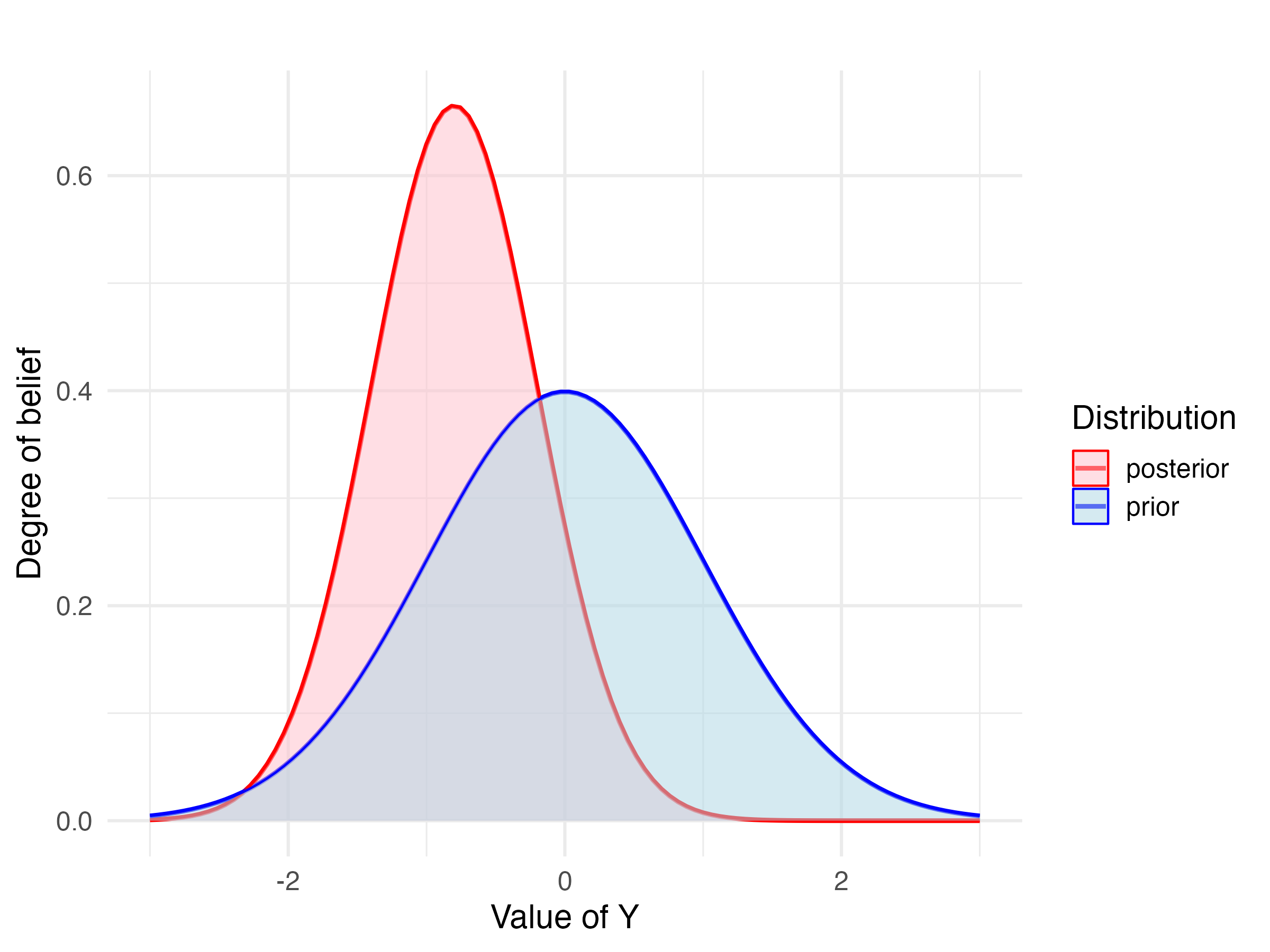
Suppose we then observe another unit, . The distance between and (or more properly, ) tells use how and will covary. If is close to , we can guess that is more likely to be close in value to . By this process, we can construct the (posterior) distribution for the unobserved . Intuitively, if takes a large value, for example, we can expect to be larger, and this information somewhat reduces our uncertainty (variance). This process is referred to as conditioning on the observations. See Figure 1, right. Scaling this logic to a set of multiple unknowns with observed covariates , and a dataset of observations , our beliefs about the distribution of the vector of for the test points is then given by
| (1) |
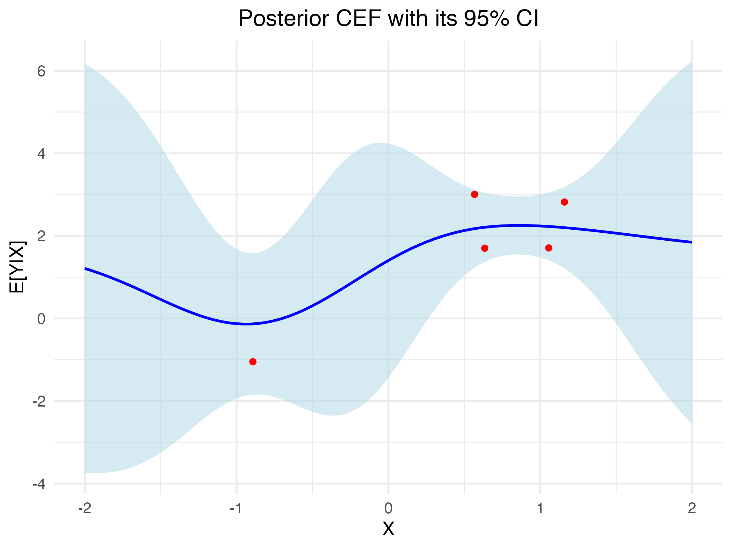
We defer derivations to Rasmussen et al., (2006) or other sources. Expression 1 can be labeled a posterior distribution for the of the test points given the data (and the choice of kernel). Further, since the normal distribution has identical mean and mode, the mean argument in posterior () is both the conditional expectation function (CEF) and the maximum a posteriori (MAP) estimator. The consequences of this expression are illustrated in Figure 2. For values of closer to observations in the data, the covariance of with the corresponding observed in the data will be higher, providing more information to revise our guess of (reduced uncertainty), whereas uncertainty will balloon farther from observed data.
Note that while such a posterior distribution could be obtained by through a markov chain sampling procedure, the entire posterior distribution for any point is available in closed-form, making such sampling procedures unnecessary. Note also that the variance in Expression 1 describes what we can believe about a point , i.e. it relates to the “predictive interval” or the standard deviation for at a point. In some contexts we are interested instead in quantifying uncertainty in the conditional expectation function (or posterior mode/MAP function), as in the standard error. The expression for the variance of this quantity is less by because it does not include that additional irreducible error.
In summary this approach shows what we should reasonably believe about the distribution of some variable with some covariates , if we (i) assume a multivariate normal distribution for the vector, a covariance structure structure that depends on as specific in the kernel function; and (ii) condition on the observed data.
Finally, to avoid confusion, we note that the model fitting procedure just described characterizes a gaussian process, but the inferential procedures invokes when using this approach will often involve additional steps. Specifically, we will use GPs in tasks that require (i) creating separate models for treated and control units for further inference; (ii) fitting models on each side of the cutoff in a regression discontinuity; or (iii) fitting data in a pre-treatment period to extrapolate into a post-treatment (test) period.
2.1 Interpretation and relationship to other approaches
To reduce notational complexity, let us look to the use of this model to fit data in a given training set without extending the predictions to new (test) locations.
| (2) |
While the left hand side describes a whole distribution, the CEF (or MAP) can be read from the mean function on the right hand side: where . This is precisely the CEF employed by kernel ridge regression techniques such as kernel regularized least squares (KRLS, Hainmueller and Hazlett, 2014). Accordingly, we can understand the functional form of the CEF using the interpretations offered by Hainmueller and Hazlett, (2014). Briefly, for example, we see that the conditional expectation of is linear, not in , but in the columns of . This implies recoding the data so that observations is understood not as but as the vector . This in turn means we are modeling as a linear function of “[similarity of unit to unit 1, …, similarity of unit to unit . As with KRLS, regularization is induced here through the . We can similarly understand it by placing a Gaussian kernel over every observation, then choosing coefficients that rescale these kernels, such that they sum up to form the CEF surface. We refer readers to Hainmueller and Hazlett, (2014) for more extensive interpretation of this function space.
The coefficients of the model linear in the kernel, i.e. the in the model , are equal to here, but denoted as in Hainmueller and Hazlett, (2014). The in that setting arises strictly as a tuning parameter governing the degree of regularization, to be chosen by a cross-validation procedure. Here it is replaced by , which has a substantive meaning (in our rescaled version) as the fraction of variance in that remains unexplained by the CEF. Further, we fit it using a marginal likelihood approach rather than cross-validation.
2.2 Outcome uncertainty estimation under model uncertainty and dependence
The key feature of this approach that makes it attractive for many inferential tasks is its ability to report uncertainty over test point outcomes or for the conditional expectation function without first committing to a single, fitted model. This mitigates model dependency concerns, subject to the modeling assumptions still made above. In this way, the GP is a useful tool to manage the dangers of extreme counterfactuals that can be highly problematic in other settings.
Backing up, conventional approaches to uncertainty estimation are constructed given a fitted model. While the variance of the estimated parameters of that model remains relevant, the model choice and fit are taken as fixed. For example, for a model linear in , the classical (spherical) variance estimate for the coefficients will be . The value of is proportional to , i.e. the sum of the squared fitted residuals.333Alternative variance estimators will have a more complex form, such as any sandwich estimator of the form , where is constructed according to some choice of assumption on the covariance structure. This does not change the fact that is constructed using fitted coefficients and residuals, so the problem remains.
Consequently, the estimated variance of the predicted value of the CEF at some point will be . Mechanically, this quantity will be larger for farther from the mean of the data. While this is somewhat fortunate insofar as we should have greater uncertainty far from the data (see King and Zeng, 2006), estimating the variance in this way has nothing to do with a principled approach of considering how uncertain we should be based on our proximity to observed data and how it informs our beliefs about at a test point. Rather, given a fixed mean and covariance of the data, the OLS-based uncertainty estimation will provide the same apparent uncertainty for a point whether it happens to be an observed point, an unobserved point near one or many observed points, or an unobserved point relatively far from any observed points.
Nor is the problem due to the rigidity of the linear model, which we can note by comparison to KRLS. While GP does provide a CEF (identical to that of KRLS), under KRLS uncertainty estimates collapse as test points are examined farther from the core of the available data. This is because the functional form of the CEF is constructed so that it will move always back towards the mean as we leave the support of the data. While this a reasonable choice for the CEF, an approach that takes the fitted model as granted and computes uncertainty estimates based on this has serious drawbacks: we will be ever more certain that the prediction of at some point far from the data is near the mean, and so uncertainty intervals will collapse. By contrast, GP does not construct estimates conditionally on the fitted CEF; it merely characterizes what we should believe about the entire joint distribution of given the observed data and choice of kernel. This result will reflect increasing uncertainty about the value of points as they move away from the core of the testing data, at least for any kernel function that is decreasing in the distance between its two arguments (i.e. those that assign lower covariance to the values of units whose covariates are farther apart, as in the Gaussian kernel). As the covariates of test points go farther from the covariates in the training data, our posterior variance for will approach . Again, the variance-covariance matrix given in Expression 1 is for the actual values of that might be drawn from such a distribution, i.e. the “predictive interval”. This is different from the variance of the CEF, given by .
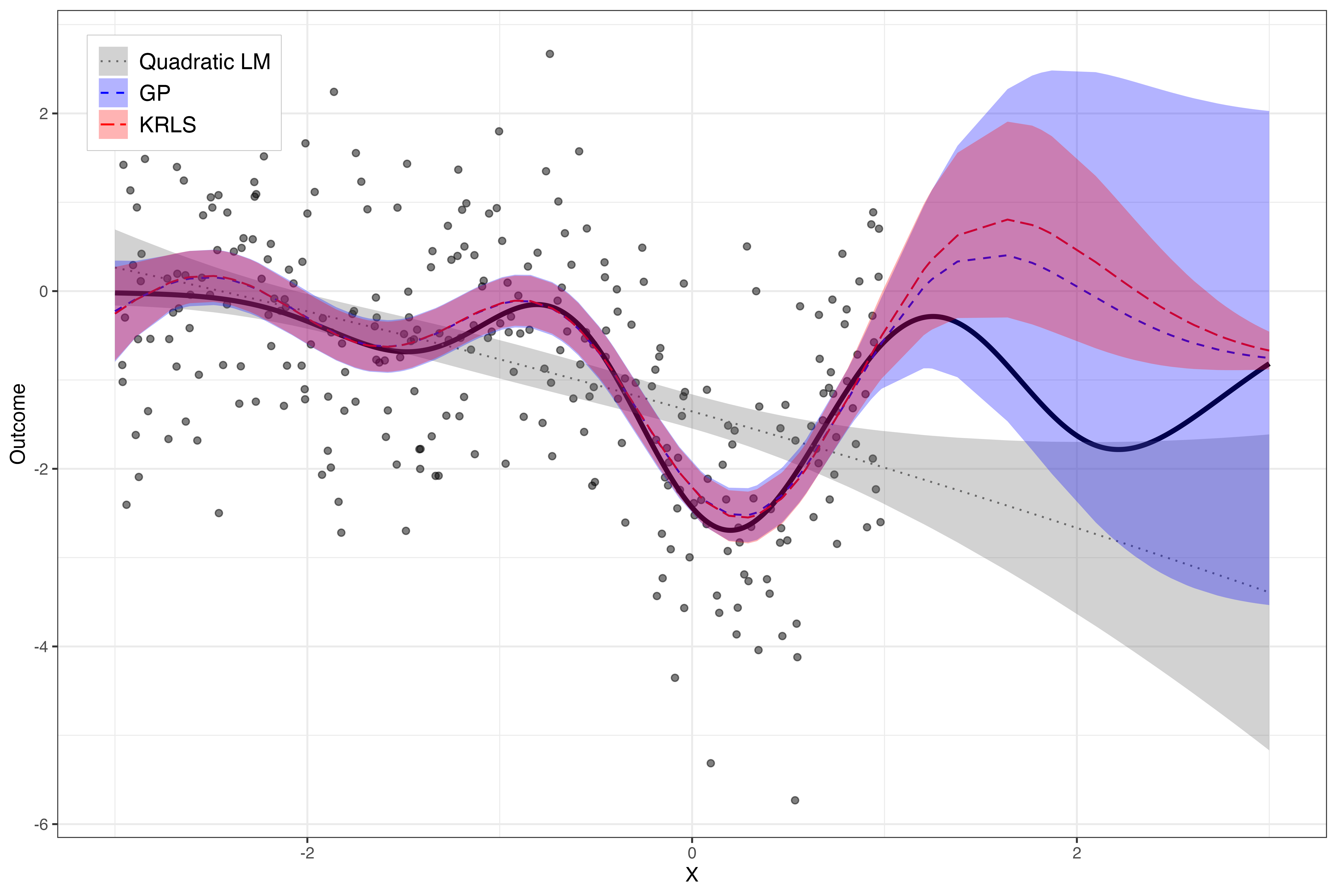
Figure 3 demonstrates these uncertainty estimation behaviors for the CEF when using OLS, KRLS, and GP as we move away from the training data. The true CEF used in the simulation is shown in black. The linear (here, quadratic in ) model shows increased uncertainty as we move away from the mean of , but this is a mechanical function of increasing the value of , and does not reflect any information related to the degree of extrapolation. Consequently, there is no reason it should expand in a way that will contain the true CEF, and indeed it does not. GP and KRLS produce nearly identical fitted CEFs with 95% CIs over the training data (). Slight differences are due only to changes in how hyperparameters are selected. Over the range of observed data. However they have similar uncertainty intervals over the range of observed data, and both contain the true CEF effectively. However, extrapolating beyond the training data to , the KRLS confidence band collapses, as described above. For GP, by contrast, our uncertainty about the value of the CEF moves back towards the “full ignorance” value as we move away from the data needed to otherwise inform it. The confidence band reflects this, growing as we extrapolate. Of the three models, only the uncertainty band for GP contains the true function throughout the extrapolated range.
2.3 Additional details
We return briefly to a number of details that are operationally important, if theoretically less interesting.
Demeaning and rescaling.
We center and scale the covariates to have unit variance. This is common for kernel approaches, and avoids dependency on unit-of-measure decisions (see e.g. Hainmueller and Hazlett, 2014). We also center and scale to have unit variance. This avoids the need for a separate hyperparameter that must be set/learned to capture this variance. Note that the variance used for rescaling can only be known from the observed sample, and the variance of the in question may be different in the range targeted for later prediction. However, this would be similarly problematic if the variance of was parameterized and to be fitted from the observed sample.
Setting .
We choose the residual variance term, , by maximizing the log marginal likelihood (Rasmussen et al., 2006)
| (3) |
Informally, this appears to perform very well empirically, in that across simulations we find the estimates is very close to 1- in the simulated DGP. That is, suppose a simulation chooses some function and data distribution , then formulates according to for each point. Then is the non-parametric for that simulation.
Kernel choice.
Kernel choice is a complicated topic, with two main domains: (i) choosing the “bandwidth” or other hyperparameters in a given kernel, and (ii) choosing among various kernel shapes.
On the first, for the Gaussian kernel , we must choose the bandwidth or “length-scale”, . There are numerous strategies for doing so. We prefer those that do not depend on the outcome data or otherwise invoking a search over fitted results for three reasons. First, they are computationally demanding. Second, there can be tradeoffs between this parameter and others in a model (such as here) such that the “optimal” value of is poorly identified. Third, we encourage thinking of this as effectively a “feature extraction” choice, which can be made on the basis of the values of without consulting . Several strategies have been proposed for choosing in the Gaussian kernel. One reasonable approach is to set equal to (or proportional to) the number of dimensions of of , which that the result does not explode or go to zero as the number of dimensions changes. In practice, this performs well. We follow the proposal of Hartman et al., (2021) to choose so as to maximize the variance of , of the variance of absent the diagonal. This simply ensures that the columns of stand to be highly informative rather than having approach the identify matrix (if is too small) or a block of ones (if is too large). In practice, this also performs well.444The way in which binary and categorical data are encoded in a kernel matrix is not always obvious. We follow developments describes in Hartman et al., (2021), which one-hot encodes all categorical values (without omitting one level) and rescales them to have appropriate standard deviations relative to continuous variables.
Regarding the kernel function itself, throughout this paper we principally rely on the Gaussian kernel because (i) it directly works with the logic that observations with more similar values should have greater covariance while covariance should drop to zero as observations grow far apart in the covariate space; (ii) it is widely considered the work-horse kernel for many machine learning approaches involving kernels; and (iii) it is an example of a “universal kernel” for the continuous functions, meaning that given sufficient data it can represent any continuous function (Micchelli et al., 2006). That said, a key feature of the Gaussian kernel is that it produces models that interpolate smoothly over the support of the training data, but drift back towards the mean near and beyond the edge of the data. In some settings, this is not advisable. For example, in a time-series extrapolation problem, we may be willing to entertain function spaces that (i) have periodic behavior, and or (ii) that can extend out linearly, quadratically, or in some other way beyond the edge of the data. We revisit these concerns in section 3.2 below, where we combine kernels so that they can employ the smoothing of a Gaussian kernel, the periodicity of a periodic kernel, and the non-stationarity of a polynomial kernel.
3 Use cases for GP
In this section we illustrate the useful properties of GPs in three settings where inferences depend on understanding uncertainty that arises from model-dependency as we move towards or beyond the edge of the observed data.
3.1 Comparing groups with poor overlap
We begin with a simple illustration relevant to covariate adjustment strategies. In cross-sectional comparisons between treated and control groups, we often need to compare the two groups as if they had the same distribution on covariates. For example, if we have an observed confounder and assume the absence of unobserved confounders (as in selection on observables/conditional ignorability), we wish to make comparisons between treated and control units conditionally on/ adjusting for .
Adjustment strategies of all kinds are vulnerable to model dependency when there are regions of that see only treated units or only control units (poor overlap). Here we consider such a condition: treated units have values of between -3 and 1, whereas control units have values of between -2 and 3. This leaves two regions with poor overlap (below -2 and above 1). The implications of this can be seen by considering a model for the outcome under treatment, and a model for the outcome under control. The model for the treatment outcome must be extrapolated in areas with few or no treated units () and the model for the control outcome must be extrapolated in areas with few or no control units (. Treatment effect estimates can be made by comparing, for each observation at its covariate location , the value of the treatment model minus the control model (i.e. g-computation, t-learner, regression imputation, etc.) For the units located in areas of poor overlap, the estimated effects may be problematic owing to the fragility of the model extrapolation.
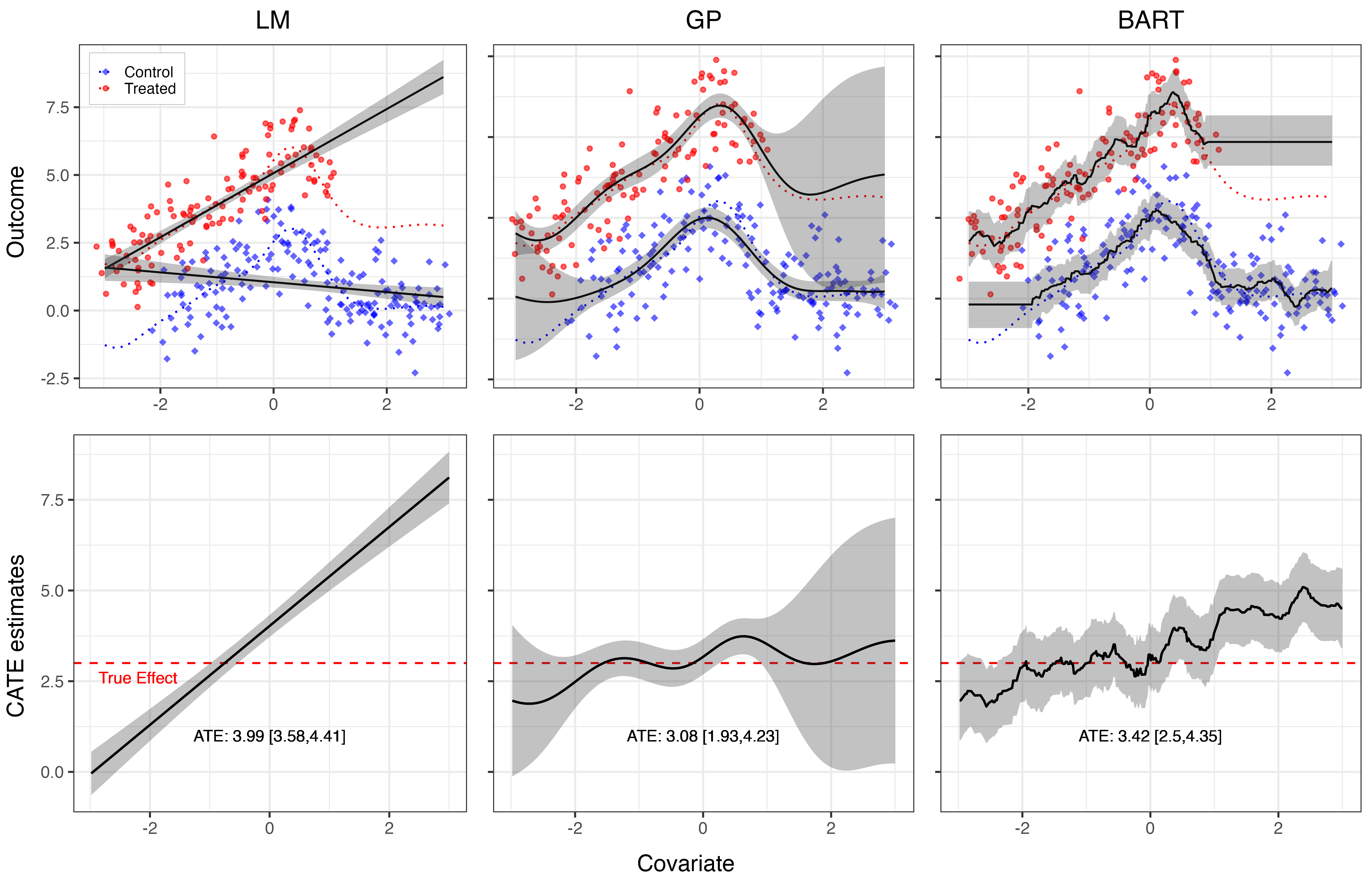
Figure 4 illustrates this concern, and the simulation setting. First, on each iteration of the simulation, we first draw a random function to serve as the CEF of given , and another for the CEF of given . Each of these is created by choosing 10 “knots” with values given by . We then choose “coefficients” according to and set “bandwidth” to . A Gaussian kernel equal is constructed over each knot point, and the random function takes the value . For the CEF of , a constant value of 3 is added to that of , so that the true average treatment effect is 3, as is the conditional average treatment effect at all values of . Following this, “observed” samples are drawn from each of these CEFs () with the addition of noise, distributed normally and with variance calibrated to ensure an overall true (between and CEF, not between and ) of 0.3. 555We set this to 0.3 in our simulations, but in Figure 4 is 0.8 to visualize our setting better.
Figure 4 shows a single example of a drawn random function from this space (black line) and simulated data under treatment (red) and control (blue). The three models tested fit the data similarly well in the region of common support (). In the regions with poor overlap ( and ), however, there are two problems: the result is highly sensitive to the choice of modeling approach, and the uncertainty estimates for LM and BART fail to show sufficient uncertainty to accommodate this model dependency with poor overlap. The bottom row of Figure 4 shows what these estimated CEFs and uncertainty intervals imply for conditional average treatment effects (CATE) and the average treatment effect (ATE). As the CATE should be constant in this setting, the apparently linear change in the treatment effect as a function of for the OLS model (left) is erroneous. This is a byproduct of the poor overlap, which led to fitted models with very different clops for the treated group versus control group. For BART, the problem is less severe, but the uncertainty estimation is still insufficient due to its underlying tree structure to accommodate model dependency in regions of poor overlap. Notice that the uncertainty over the CATE remains nearly constant for BART across areas of good overlap and poor overlap, which is concerning as well. For GP, while the fitted model shows some drift, the uncertainty estimation appropriately accounts for potential model dependency and our limited knowledge of what happens outside the range of common support. Notice that this additional uncertainty is not global—the GP result is fairly precise over the region with common support while exploding where there is poor overlap.
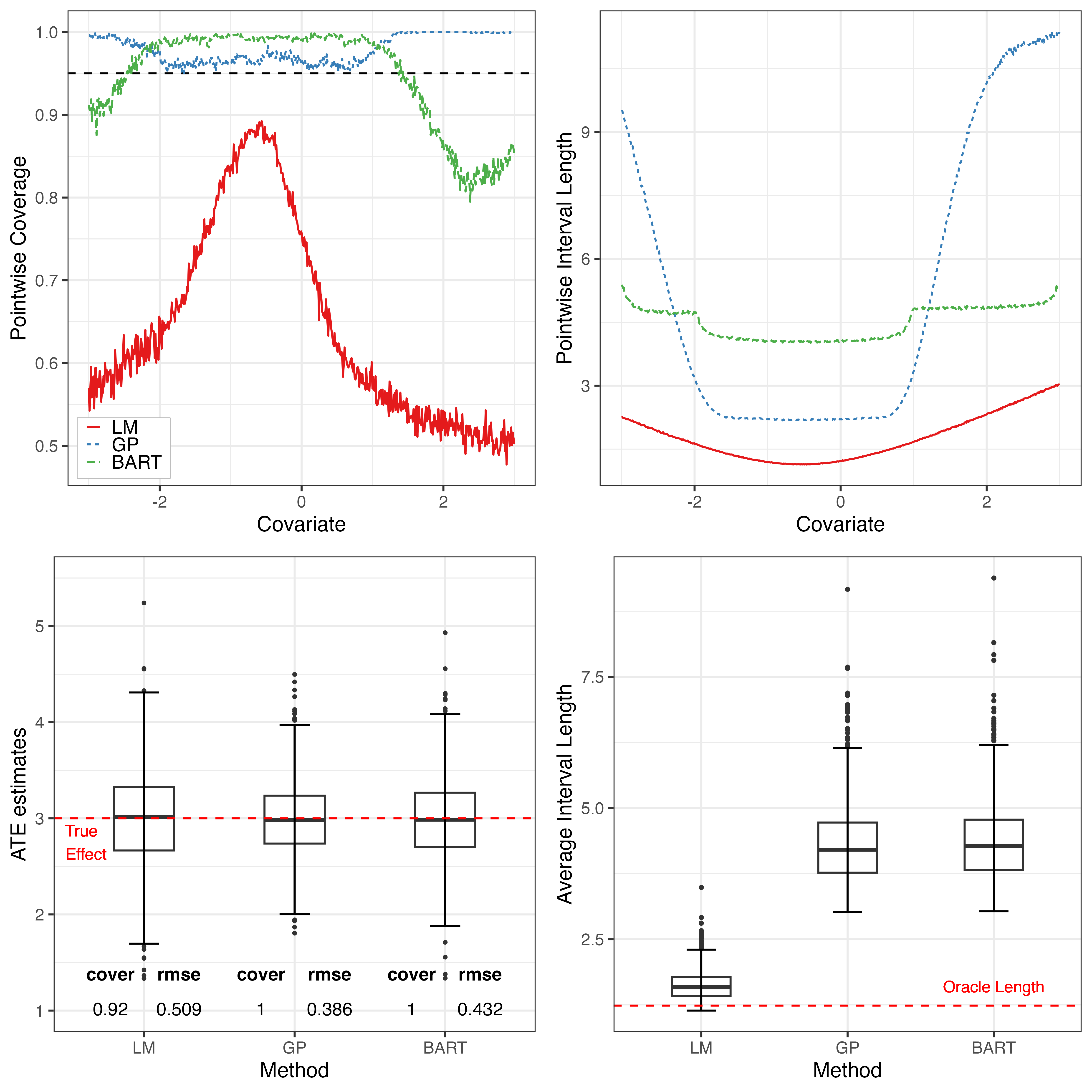
We then repeat this process over many different random functions that could be drawn in this way. Figure 5 demonstrates the behaviors of each method across 1,000 iterations, generating separate random functions each time, with sample sizes of 500 according to the description above. The coverage rate for the CATE at each possible value of (top left) is problematic for the linear model at all values of . BART has over-coverage in the area of common support, but under-coverage in areas of poor overlap. The GP approach produces nearly nominal coverage in the area of good common support then transitions into over-coverage in areas of poor overlap. This is perhaps desirable, conservative behavior for many purposes. The interval lengths required to achieve this (top right) are also of interest. The drastic under-coverage of LM results from inappropriately short intervals at locations in . BART has moderate (almost constant) interval lengths throughout. GP has narrow intervals in the region of good overlaps, despite achieving nominal coverage there. The interval lengths grow wide, as expected, to achieve the over-coverage observed in areas of poor overlap. We also examine the implications of these approaches for the ATE estimates themselves. Across iterations, the RMSE of the ATE estimates for GP is only 76% as large as that of LM, and 89% as large as that of BART (lower left). Both BART and GP over-cover the ATE, whereas LM has under-coverage. This comes at the cost of larger intervals (lower right).
3.2 Interrupted Time-Series with GP
Background.
The ITS design is used in social science and public health studies to assess the effect of events or shocks experienced by everyone after a given time (Box and Tiao, 1975; Box and Jenkins, 1976; Bernal et al., 2017). In the interrupted time-series setting, we observe a time-series for some variable () beginning prior to some event of interest. The outcomes at these times can be regarded as non-treatment outcomes, . At time , an event occurs, such that all outcomes measured after that time are treatment potential outcomes, . We suggest a simple imputation approach to the ITS design. A model for the non-treatment outcome is trained on the pre-treatment outcomes then extrapolated to the post-treatment era for imputing non-treatment counterfactual outcome, where it can be compared to the observed (treatment) outcome in order to attempt a causal claim. The GP approach is promising in this arena for several reasons. First, it naturally encompasses auto-correlation in the outcomes. Second, as we will show, the covariance function (kernel) can be designed to accommodate not only the “smoothness” implied by expecting observations closer in time to have higher covariance, but also secular trends that will continue on over time and periodic trends such as seasonality. Third and most relevant to our discussion, a central difficulty with ITS is that it always requires extrapolating well beyond the support of the data, and so is highly vulnerable to model dependency. Hence, the management of uncertainty in GPs is desirable, in contrast to approaches that compute uncertainty estimates conditionally on the residuals from a fitted model.
Combining kernels.
The covariance function (kernel) encodes our expectations about the regularities of a function we wish to learn. For instance, a linear kernel makes assumptions about linear relationships, a periodic kernel encodes cyclical patterns, and a Gaussian kernel models smooth trends. Multiple kernels can be combined via addition (or multiplication) operations to produce new valid kernels with different properties (Schulz et al., 2017). This allows us to incorporate as much high-level structure as necessary into our models. We will use a combined kernel that adds a linear, periodic, and Gaussian kernel in order to identify a combination of temporal patterns in our data, i.e., a long-term linear trend with some obvious seasonality and local deviations. In doing so we attempt to explicitly model the data as a sum of independent processes (Duvenaud et al., 2013). We will limit the maximum number of base kernels to three and do not allow for repeated use of base kernels for tractability and reliability of hyperparameter tuning.
Causality.
The difference between observed post-treatment outcomes and extrapolated non-treatment outcomes at a given time can only be interpreted as the causal effect of that event insofar as the predicted values closely represent what would have truly happened absent treatment. This can be understood as requiring two constituent assumptions. The first is that the (possibly high-ordered) trend information required to effectively model in the post-treatment period was available in the pre-treatment period and sufficiently well picked up and utilized by the model. The second is that no “other event” relevant to the outcome occurs within the comparison period after treatment. That is, if some event not considered the event of interest occurs and influences the outcome, it will influence , and a proper causal contrast would utilize the so affected. However, since this information was not available in the pre-treatment outcome, it cannot be added into the estimate of . Although it is a substantive and untestable question, we will limit our attention to short-term post-treatment periods to minimize the concern.
Illustrative application.
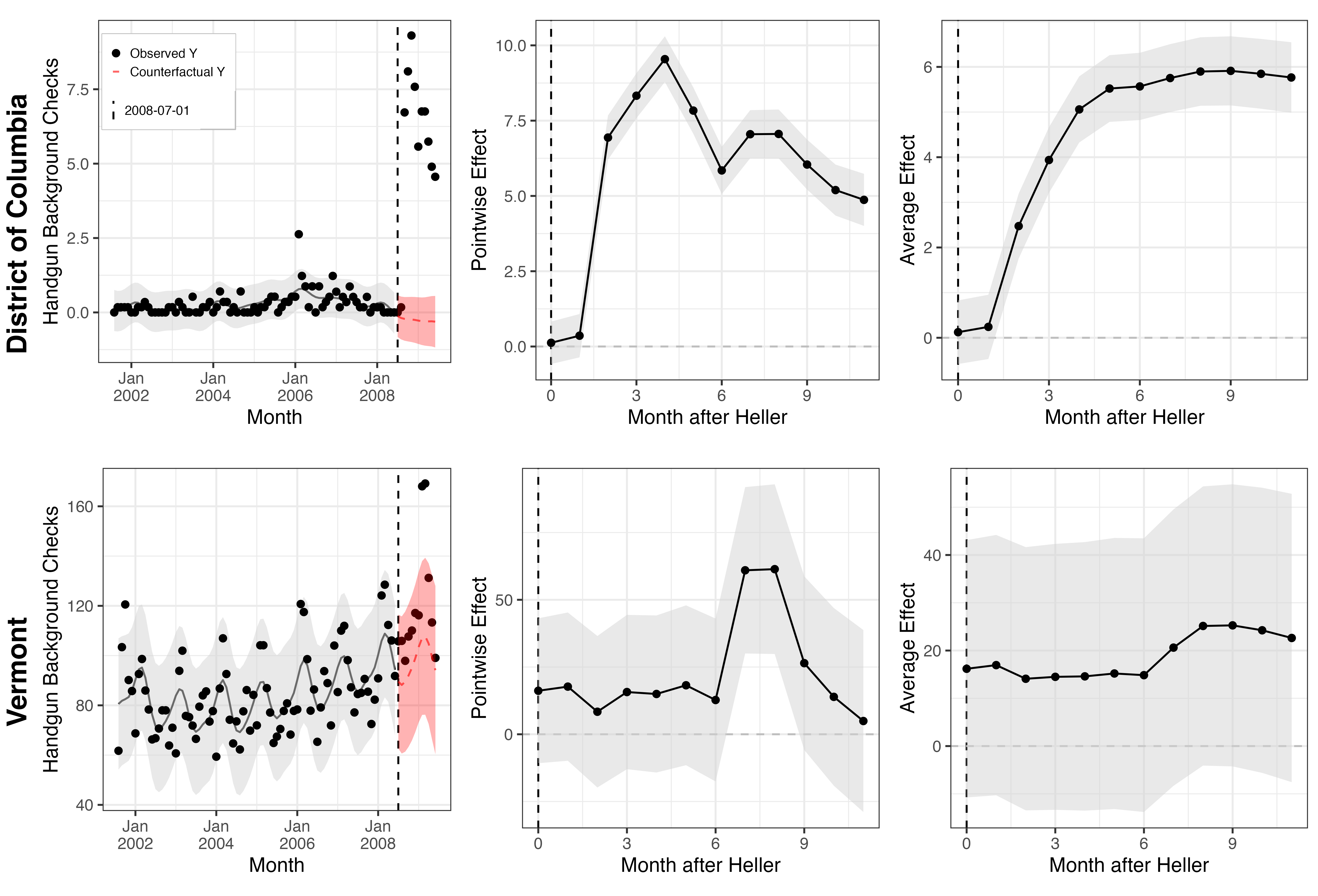
In June 2008, the Supreme court ruling in District of Columbia v. Heller, 554 U.S. 570 (2008) affirmed the individual’s right to keep and bear arms for self-defense and other purposes, striking down DC’s prior ban. We examine how the number of handgun background checks per 100,000 population (as a proxy for handgun sales) may have responded to this decision.666Thanks to Jack Kappelman for these data.
Figure 6 shows results for DC and Vermont, learning the pre-treatment trajectory from seven years of data (July 2001 to June 2008), and showing one year of post-treatment outcomes (July 2008 to June 2009). In DC, the increase in background checks immediately after Heller is substantial compared to the expectations suggested by the GP model, even given the additional uncertainty due to extrapolation. Again, this should be regarded as causal only subject to the assumptions noted above, and notably that “nothing else new and of interest happened” in this post-treatment period that is therefore missing form our model for . One cause for concern is the inauguration of President Barack Obama in January 2009, which may have also influenced handgun purchasing. That said, the increase in sales seems to pre-date either the inauguration or the November 2008 election result, while closely fitting the timing of the Heller decision.
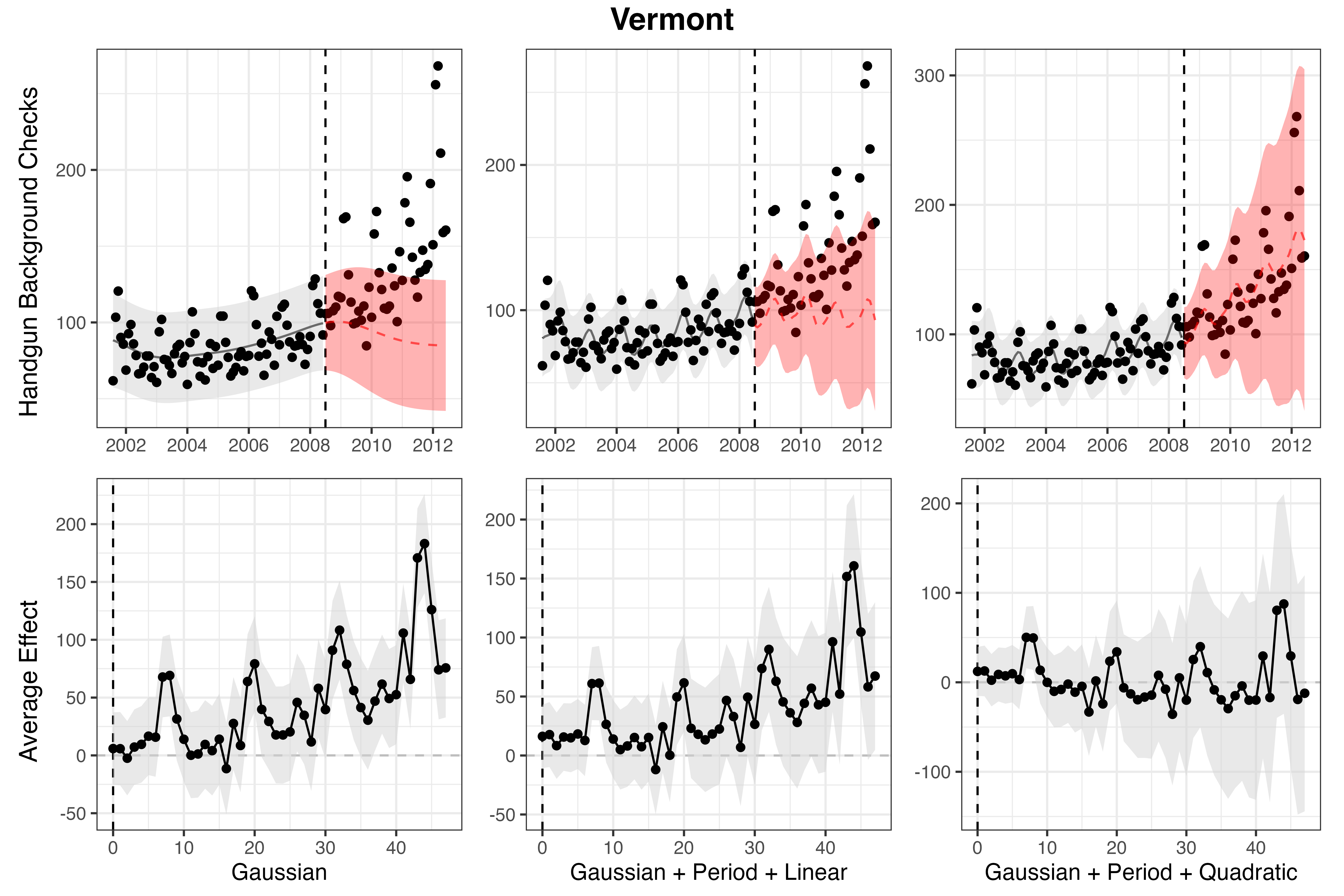
In the case of Vermont, the results are not as clear. In Figure 6, many but not all points in the post-treatment period fall within the interval expected post-treatment, leaving to some time points that show significant effect estimates while many others do not (bottom, center). Further, Figure 7 emphasizes that the conclusions one reaches depend on what one is willing to assume about the function space used to extrapolate forward. Building on the Gaussian plus periodic kernel (with one year cycles), then even adding a linear (non-stationary) component to the kernel function still suggests that many of the post-treatment observations would be unexpected under the anticipated distribution of in the post-treatment period (middle column). However, if we cannot rule out quadratic growth in the underlying trend, then we cannot rule out the posterior distribution over time shown in the right-most column of Figure 7. The lesson we seek to emphasize here is that assumptions made about how may evolve over time (i.e. linear versus quadratic) are causal assumptions from outside the data, and the conclusions we can make and defend depend upon such assumptions. We argue that GP is then suitable technology for showing us the reasoned implications about such an assumption for our beliefs about the distribution of the post-treatment outcomes under any choice of such assumptions.
3.3 Regression discontinuity
The regression discontinuity (RD) design is now widely used in the social sciences. This approach applies where decisions about treatment turn on a sharp cutoff in some variable, often referred to as the running or forcing variable. This comparison of units just below this cutoff to just above it may retain some bias due to differences in that and other characteristics, but near enough to the threshold, should be dominated by any effect of treatment. Classic examples include the use of sharp cutoffs in test scores to determine scholarship eligibility (e.g. Thistlethwaite and Campbell, 1960), or the use of electoral margin of victories to determine who wins an election (e.g. Lee, 2008). We refer readers to existing sources such as Cattaneo and Titiunik, (2022) for recent reviews of this approach.
The RD approach is unusual in that the identifying assumptions it requires are relatively weak and credible in many settings, but the estimation challenges are non-trivial. On identification, a suitable assumption is that (the conditional expectation function of) the potential outcomes is continuous in at the cutoff (). See Hahn et al., 2001 for seminal work on this, together with more recent reviews such as Cattaneo and Titiunik, (2022). While this is untestable, it is more credible than the identification assumptions on which most strategies rest, so long as no treatment other than that of interest occurs at the same cutoff. However, estimation challenges remain. Through the lens of this paper, the principal challenge is that the RD framework always requires making a prediction from the “edge” of the data. One model is needed for the outcome expected at the cutoff based on data below the cutoff, and another for the outcome expected at the cutoff based on data above the cutoff. Data very near the cutoff may be sparse. Difficult decisions must be made regarding the bias-variance tradeoff in such models: how much should we benefit from data that is not as near to the cutoff, given that including such data can bias our estimate? Even when optimizing this choice by some criterion, the consequent bias must be dealt with when estimating uncertainty. Stommes et al., (2023) reviews varied approaches to dealing with this bias and its implications for inference. Among such approaches, Calonico et al., (2014) provides a now standard approach to optimal bandwidth selection, bias-adjustment of the point estimate, and bias-adjusted inference, which we refer to by the name of the subsequent software, rdrobust Calonico et al., (2015, 2017).
In this paper, we examine the usefulness of GP approaches when quantities of interest require making estimates at or beyond the edge of the supporting data, making RD a natural application. The GP approach is attractive as an alternative to local polynomial fits with bandwidth optimization or other approaches because (i) with a flexible kernel (e.g. the Gaussian) it makes only weak assumptions about the smoothness of the conditional expectation functions, and (ii) it accounts for uncertainty (over the expected outcome at the cutoff from each model) by asking what we can rationally believe about its distribution given the nearby information, within the commitments of the GP framework. In this way, it again breaks with approaches that fit a particular model, with or without a bandwidth/model selection procedure, and employs the fitted residuals directly. While conventional approaches thus omit uncertainty related to model/bandwidth selection once that model/bandwidth is chosen, the GP approach simply offers to tell us what we can believe about the predicted outcome at the cutoff, given the presumed normal distribution and choice of kernel/covariance function.
We expect that approaches such as rdrobust are ideal when their requirements of relatively large sample sizes, as noted by Calonico et al., (2014), are met. Unfortunately, in practice investigators may be limited to smaller sample sizes. In political science in particular, relying on elections can be limiting depending on the number of electoral units and cycles, compounding by the potential scarcity of the close elections on which the estimates depend most heavily. Stommes et al., (2023) find that, indeed, political science studies RD may be pathologically under-powered and show evidence of inappropriately narrow confidence intervals. The GP approach may thus be useful as an alternative that produces well-founded inference when samples are smaller than hoped for in RD studied, within the constraints of the GP framework (i.e. given a kernel function and the Gaussian distribution assumed). Below, we consider several simulation and real data applications to examine the behavior of the GP approach to RD estimation. We find that in these settings GP generally performs very well and is comparable to rdrobust in medium to large samples, albeit with slightly more conservative coverage rates whilst also maintaining lower RMSE. In smaller samples, it appears to be far more reliable, as anticipated.
RD case 1: Total random simulation.
As an initial investigation, we consider the simple “total random case”, in which the running variable () and the outcome () are both drawn independently at random. This ensures no treatment effect for any unit. Specifically, for each of 1000 simulations, we draw a sample of size 500, with , and . The value of is varied from near zero up to 3, reflecting various possible scaled of the outcome variable relative to the forcing variable. We use a cutoff of 0 for to determine treatment eligibility status. The rdrobust estimate employs the software defaults and utilizes the “robust” estimates, meaning the bias-adjusted point estimates with the robust choice of confidence intervals. To compute the GP estimate, GPrd we
-
•
use our GP function with defaults to model given using only the data from (the “control” sample) and separate from data where (the “treated” sample).
-
•
use each of these models to predict at precisely
-
•
the difference between these two point predictions is the estimated treatment effect.
-
•
the standard error for this estimate can be computed by calculating the square root of the sum of the variances of the two predicted outcomes.
(a) True effect of zero,
(b) True effect of three,
(c) True effect of zero,
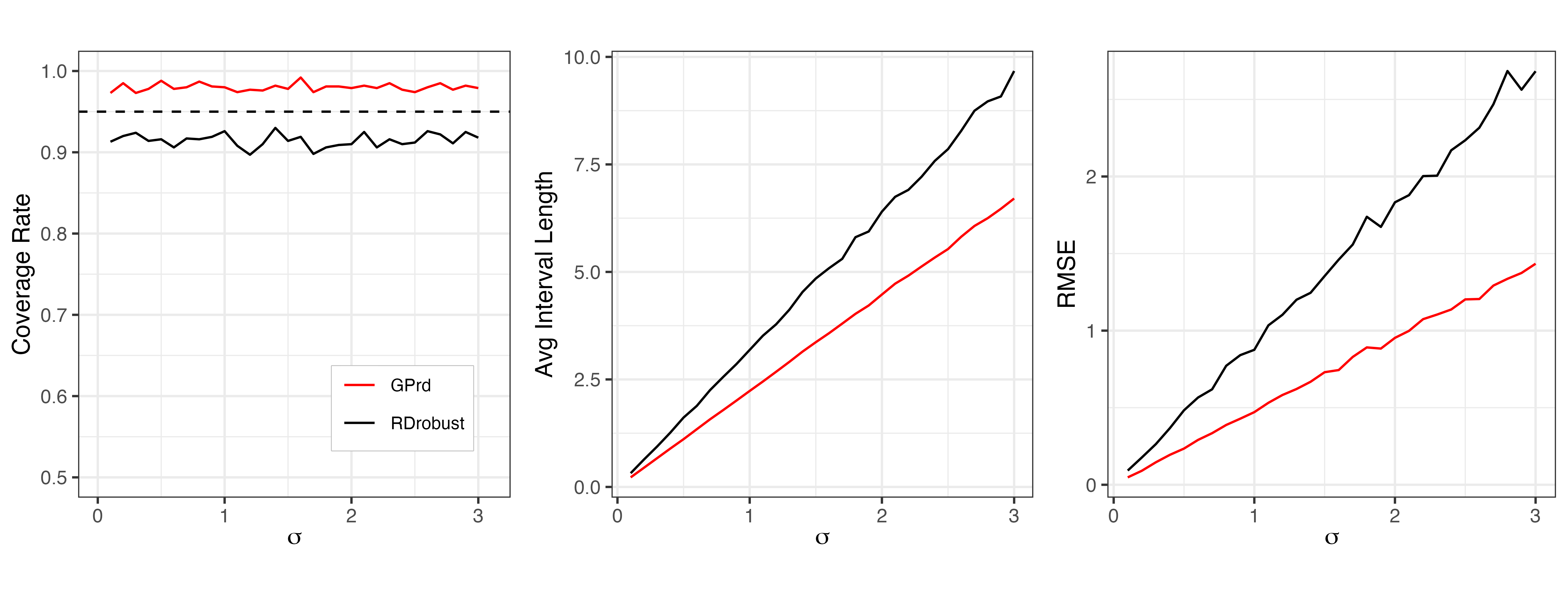
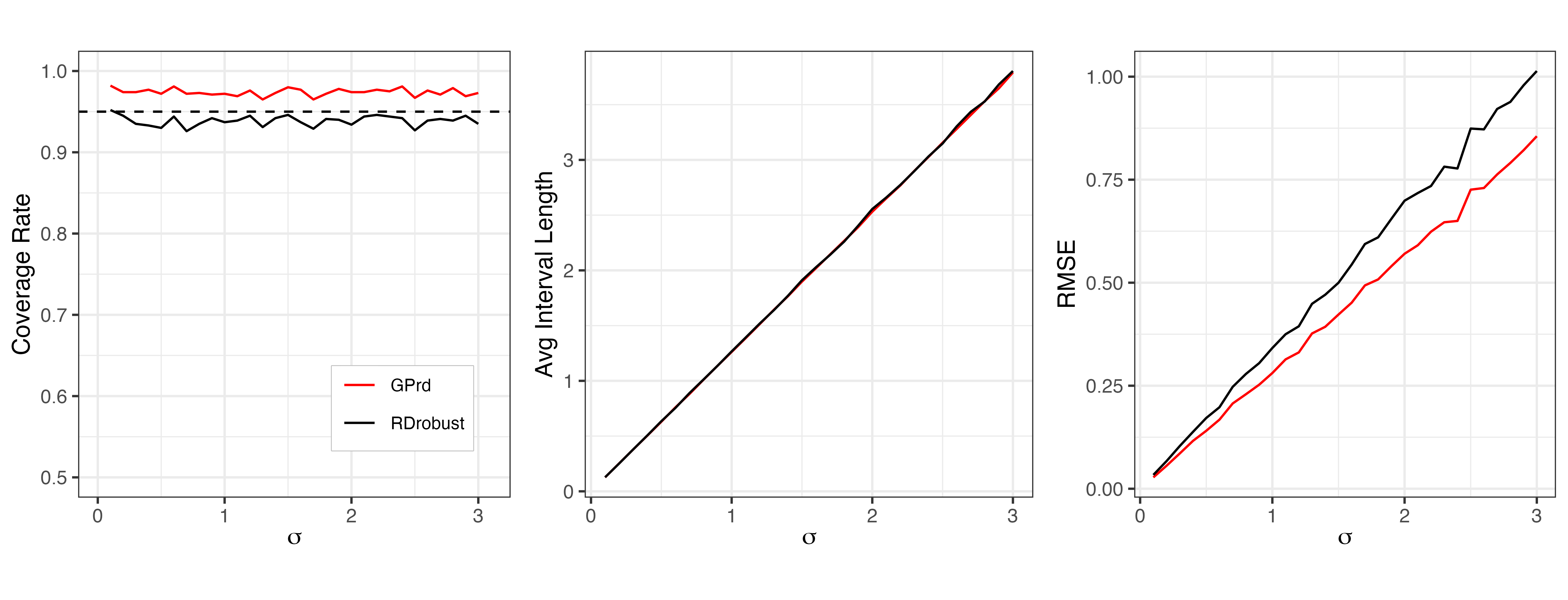
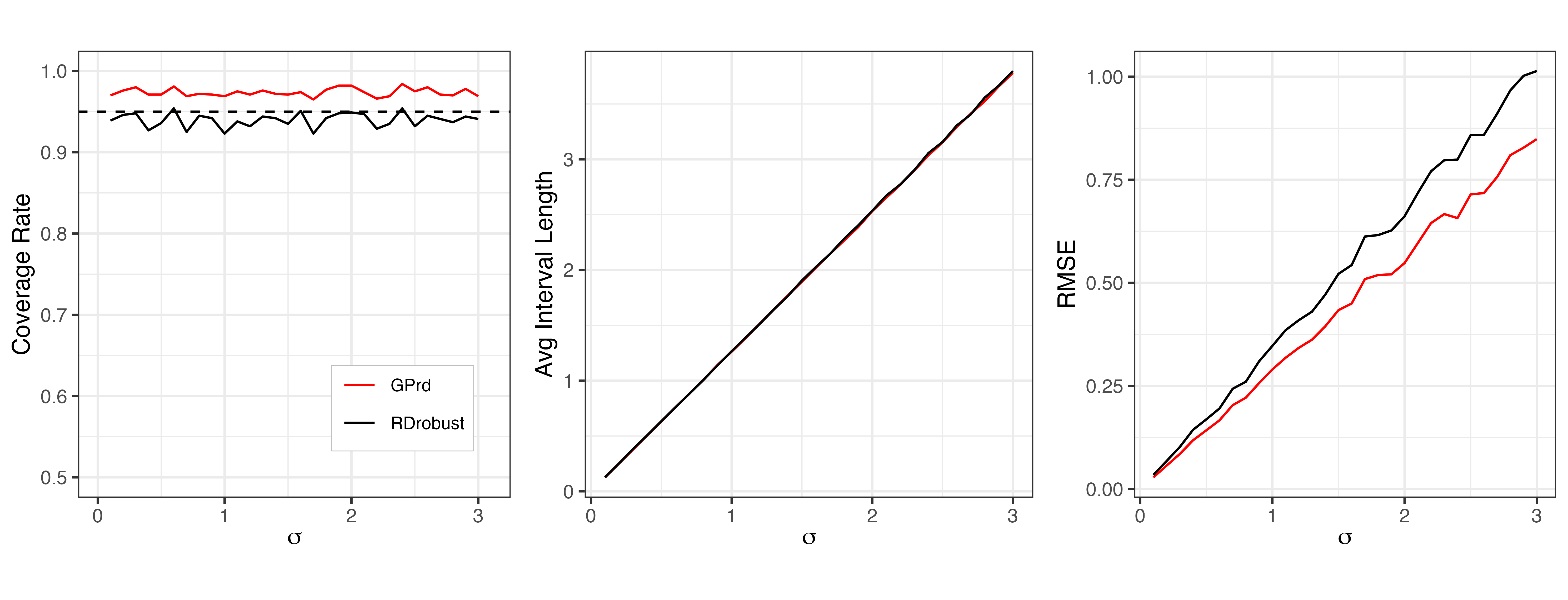
Figure 8 shows the summary of simulation results. Looking first to the upper row (where the true effect is zero), we see that GPrd has a higher coverage rate than rdrobust across different levels of variance of relative to (indicated by on the horizontal axis). For GPrd, the coverage rate is between 97% and 99%, while rdrobust has a coverage rate between 91% and 94%. The two approaches have essentially identical interval sizes, which appropriately scale linearly with (middle). Despite having the same interval length, GPrd also shows smaller RMSE across the 1000 simulations. This combination suggests lower average bias of GPrd compared to rdrobust. One concern this raised is that perhaps GPrd is biased towards zero, thus producing superior performance on a simulation where the truth was zero. We thus repeated the simulation but adding to all treatment outcomes so that the true effect size would be non-zero. This produces the same conclusions (Figure 8, middle row).
Finally, we repeat the analysis reducing the sample size to to exacerbate the small sample concern (Figure 8 bottom row). Again GPrd shows sufficient coverage with smaller interval lengths and roughly half the RMSE of rdrobust, making it a potentially useful approach in settings where the sample size is inappropriate for existing approaches.
RD case 2: Latent variable confounding simulation.
The total random case is a useful starting point, but may not produce sufficient risk of bias because there is no relationship between and on either side of the cutoff such that incorporating information farther from the cutoff risks adding bias to the estimate. To better simulate this concern we consider a latent confounding formulation. In each of 1000 replications, we generate a random sample with size 500 according to the following:
-
1.
Draw a latent variable: .
-
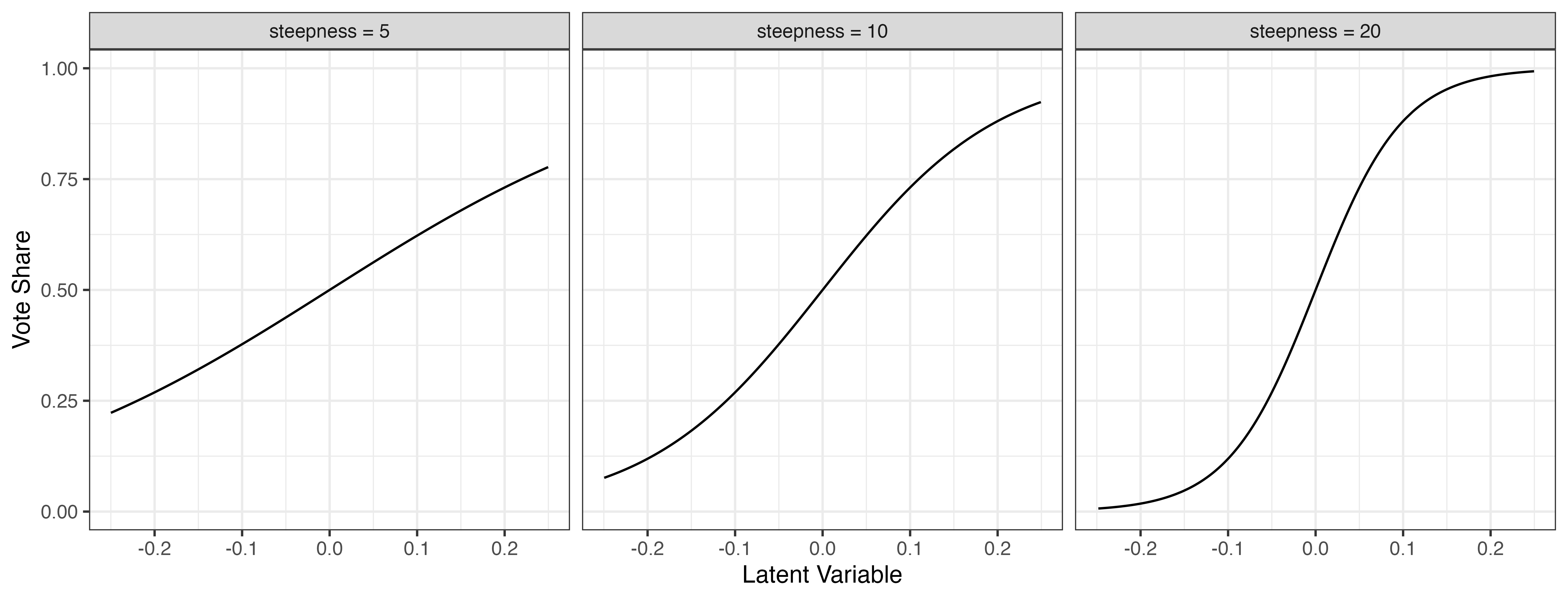
2.
Create our running variable, , representing vote share in an electoral RD as a sigmoidal function of , with . The parameter represents a varying degree of steepness of this sigmoid, such that larger values produce a steeper sigmoid, increasing the risk of bias due to misspecification. See Figure 9.
-
3.
The treatment is winning the election, , coded as 1 if the vote share is greater than 0.5, and 0 if less than or equal to 0.5.
-
4.
Generate the outcome where . This indicates a true treatment effect of three. The will be varied by simulation setting to explore a range of realistic signal to noise ratios.
With such simulated date we consider additional estimators. The first is the same GPrd approach described above. However, we also consider here whether the estimation approach should itself involve causal assumptions, i.e. those from outside the data. In any purely data-driven approach, such as GPrd or bandwidth optimization as in rdrobust, it is possible that choices are made that will put considerable weight on data farther from the cutoff than an investigator would believe is credible if our aim is to exploit the sharp cutoff. An alternative is to integrate an assumption about “how far is too far” into the estimation process. To this end we consider options that set the bandwidth or trim the sample (or both) based on outside assumptions:
-
•
gp_causal: The investigator uses substantive knowledge to manually set the bandwidth of the kernel function, i.e. the covariance of as a function of the running variable. In our close vote election simulation, for example, it might be reasonable to propose the correlation two points whose vote shares are 2% away may be correlated highly, e.g. at 0.9. This implies a surprisingly small value for b at 0.005.777. Correlations equal covariances here due to the rescaling of the outcome. The running variable is not rescaled, so that the 0.02 in the numerator remains correct.
-
•
gp_causaltrim: After choosing a bandwidth as in gp_causal, trim the data set so that regions that are effectively irrelevant to estimation at the cutoff are removed. This aids in transparency, but is also useful because the residual variance term in the GP () is a single global parameter, so trimming the data first ensures it is determined over the range of the sample that is relevant, whereas including data far from the cutoff may produce skew the value if outcomes are much more or less noisy in those regions. In our simulation, we remove observations with vote shares below 0.4 or above 0.6, on the premise that users would likely argue that data outside this range are of no value to modeling what happens at the cutoff.
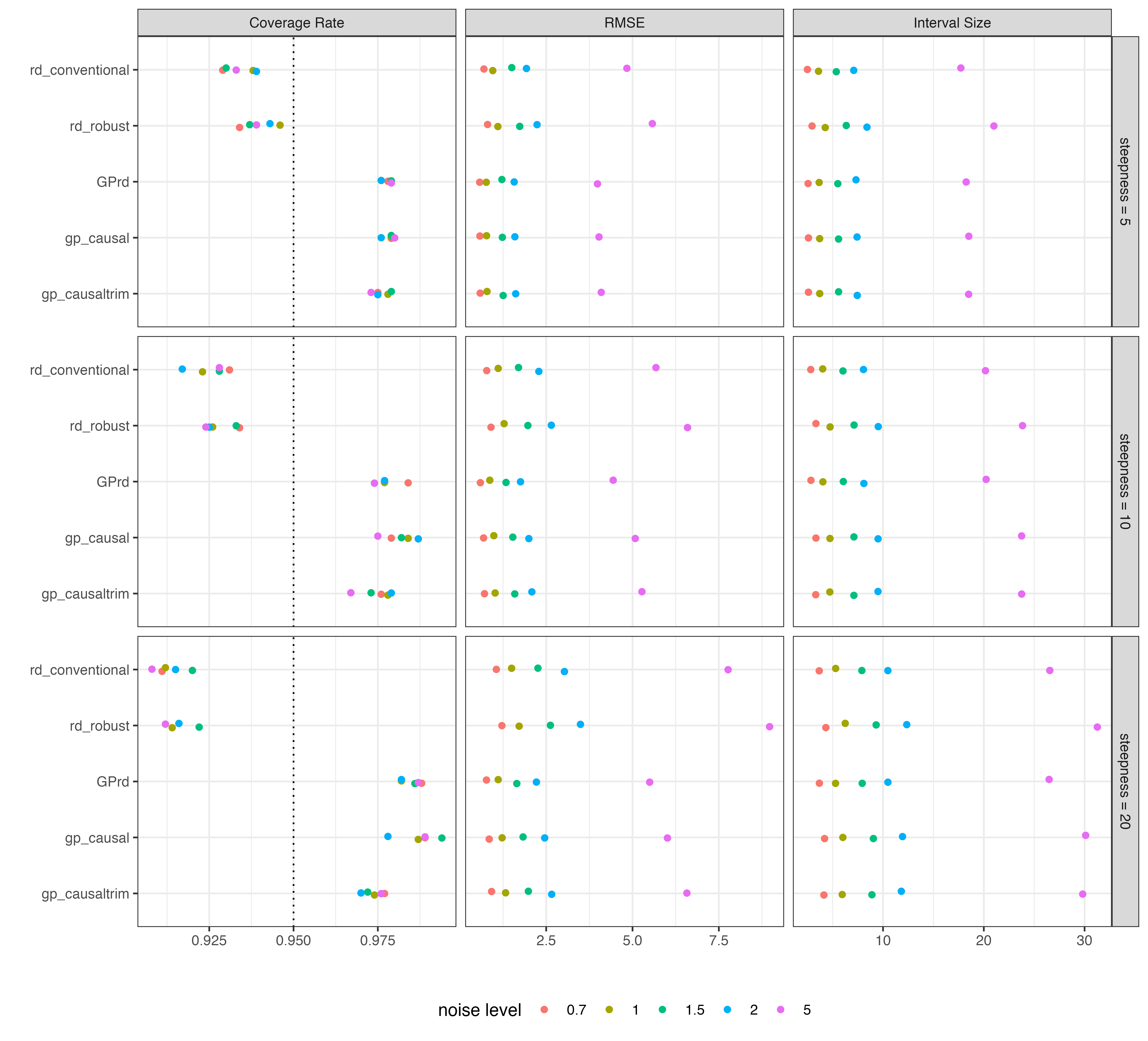
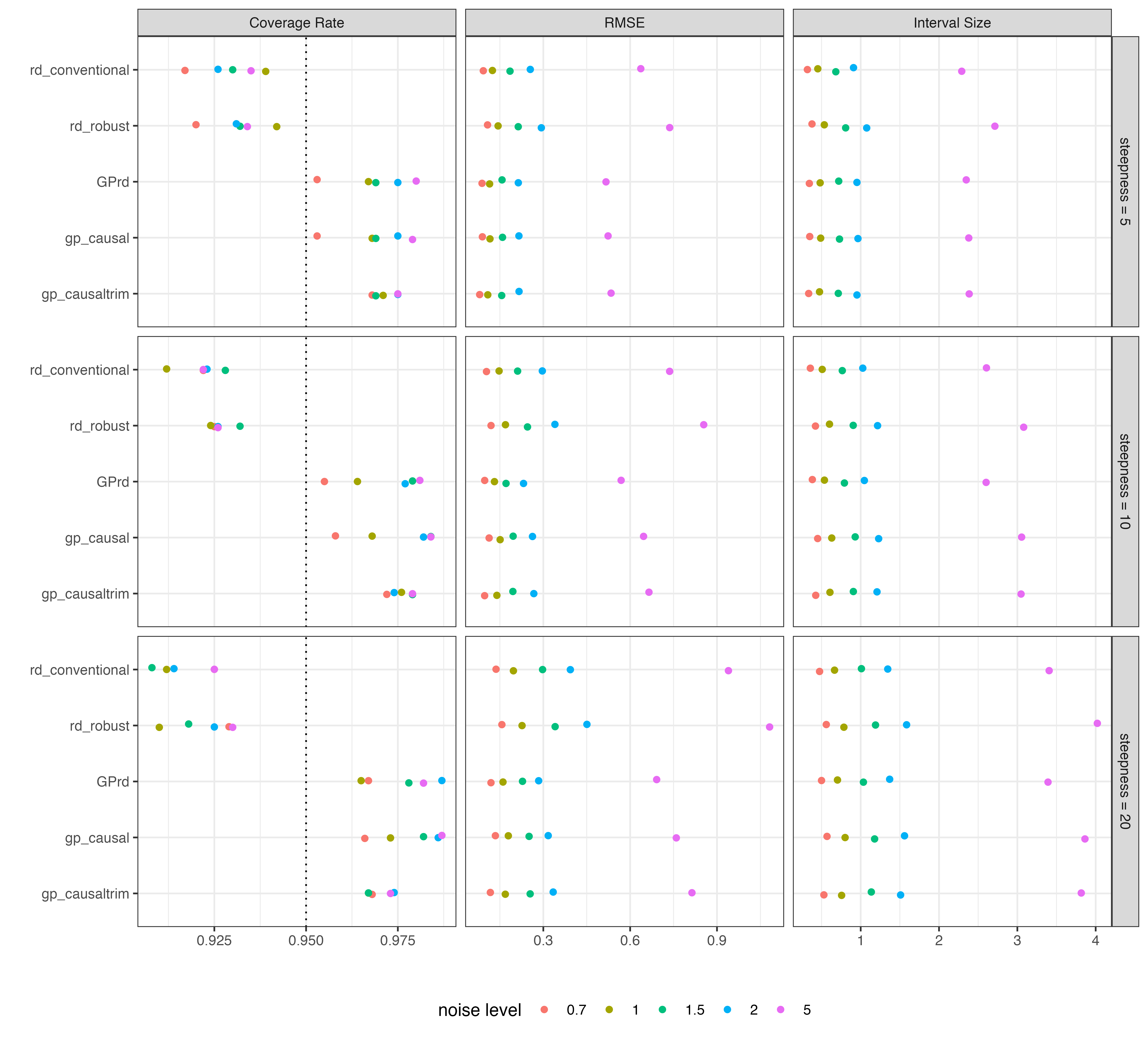
Figure 10 summarizes the results over 1000 iterations at each choice for the steepness () of the latent relationship between and and at five different noise levels that vary the true and thus the influence of on . The pattern is consistent across these settings: all the approaches show similar interval sizes and RMSE, but the rdrobust approaches (conventional and robust) generally undercover slightly, while the GP-based approaches slightly over-cover. There is little difference between the various GP-based approaches. gp_causaltrim is appealing in that provides clarity and transparency in what data are employed and the presumed covariance as a function of the distance between points.
RD case 3: Empirical application with benchmarking by placebo cutoff
Finally, we seek to study performance on real data, but in a case where the true correct estimate is known. To do so, we consider the data from Lee et al., (2004), in which the forcing variable is Democrats’ (two-party) vote share in US House Election (1948 - 1990), and the outcome of interest is a measure of how liberal each representative’s vote record is assessed to be, called the ADA score. We consider not only the actual effect estimate, but also a series of eight placebo estimates formed by pretending the cutoff on two-party vote share to win is something other than 0.5. In each such analysis, data are included only from below 0.5 or above it, but not from both, in order to avoid skewing the result due to a real treatment effect. At these placebo cutoffs, we hope to find no discontinuity effect of crossing those cutoffs, and finding such an effect would be troubling.
We consider three estimators: the GP estimator at defaults (GPrd), the GP approach with additional “causal” assumptions on the bandwidth and trimming (gp_causaltrim), and the rdrobust approach with the “robust” choice of estimates (rdrobust).
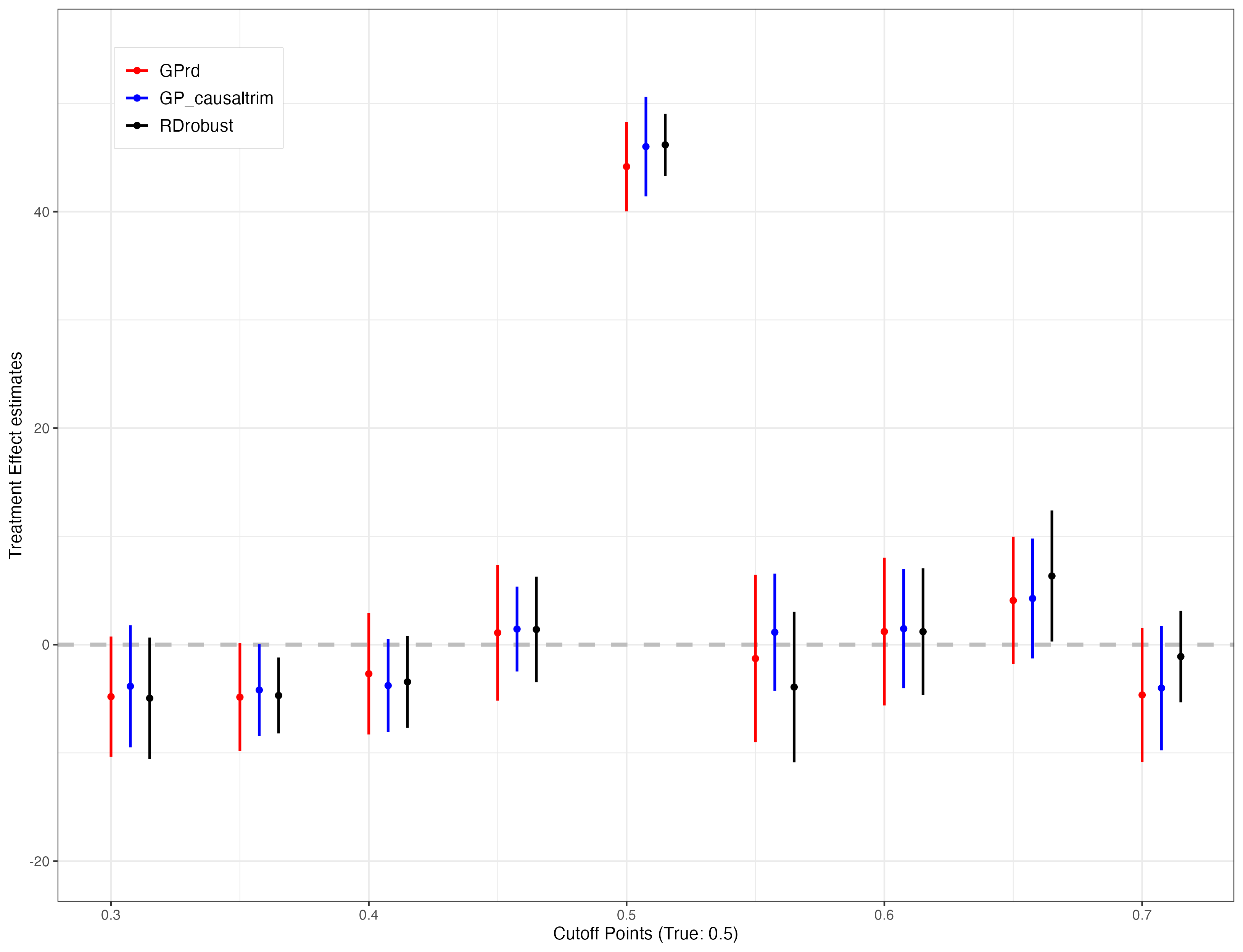
Figure 12 shows results with the full data. As shown, the choice of estimator matters little here to the answer obtained at the true cutoff (0.5), though GPrd and gp_causaltrim are somewhat more cautious in their confidence intervals. Looking at the eight placebo cutoffs, the differences are relatively small and while rdrobust suggests a statistically significant estimate at the cutoff of 0.35, GPrd and gp_causaltrim very nearly do as well. At the cutoff of 0.65, the rdrobust interval again excludes zero, while the intervals for the GP approaches do not, but the difference is again relatively small.
However, the Lee et al., (2004) data initially contains 13,577 observations without missingness on the running variable and outcome. While each of the placebo cutoff analyses uses only a subset of these points, there are still thousands of observations available to each of these estimates. The similarity of the GP and rdrobust approaches in this context is reassuring. Of greater interest in our analysis is the question of whether GP provides a suitable approach to RD in sample sizes that may be too small for the rdrobust or similar approaches. We thus use the same data as the basis for a second analysis in which we examine much smaller sub-samples. Specifically, we
-
•
fix a (placebo) cutoff point: 0.3, 0.4, 0.5, 0.6, 0.7 (0.5 is the true cutoff)
-
•
limit the data to just 0.1 above and below the cutoff in question (e.g., for cut=0.4, data with are used) to maintain symmetry and comparability across cutoff estimates
-
•
sub-sample 200 observations (without replacement) from the remaining eligible observations
-
•
estimate treatment effect using various models
We repeat this 2000 times. The resulting estimates can be used to demonstrate the distribution of point estimates under resampling in this way. We also report coverage and RMSE, in both cases taking the “full sample” estimates above as the true/long-run target.
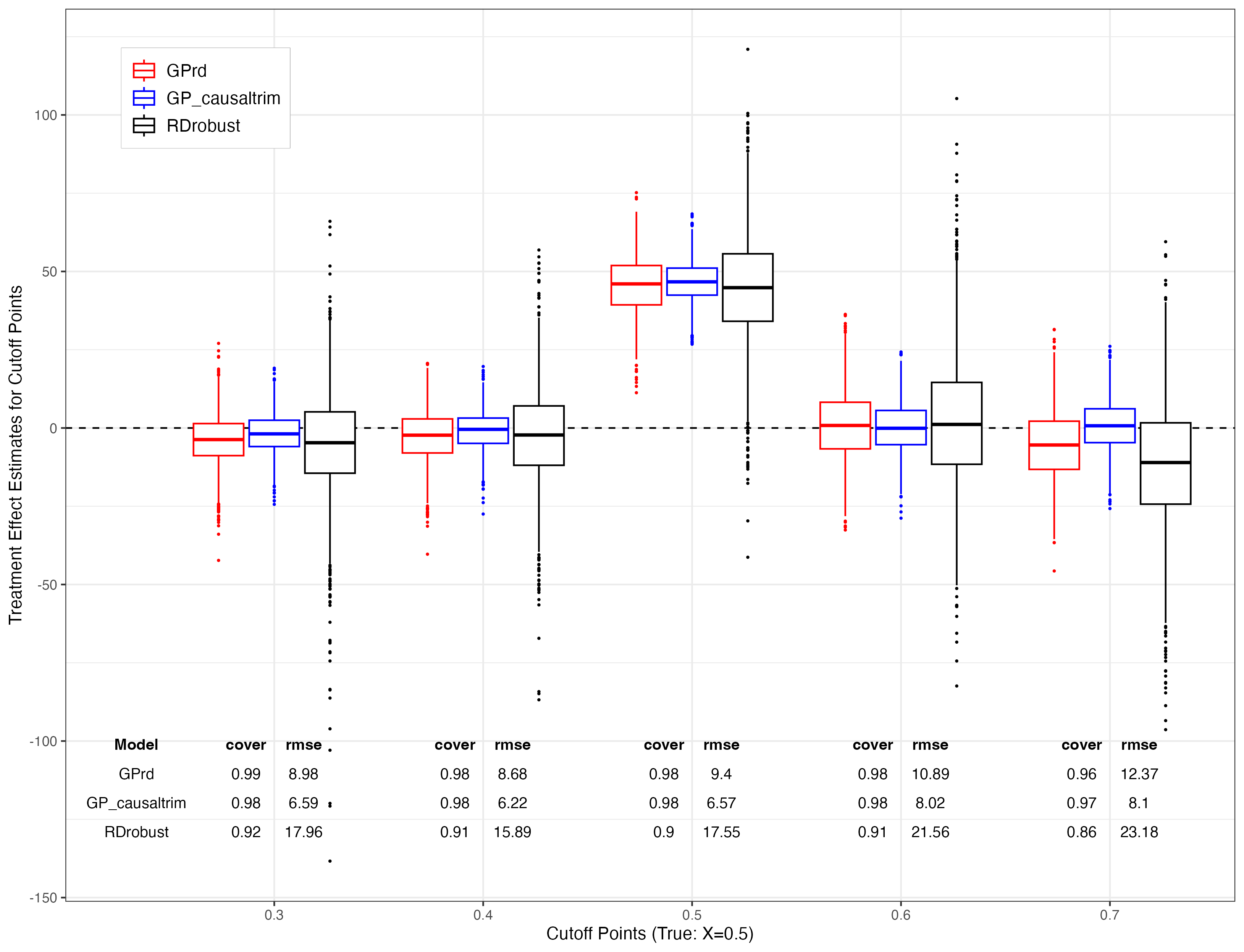
Figure 13 shows the results. In general, the GP approaches are similar, with gp_causaltrim showing somewhat narrower distributions. As this approach makes stricter (and arguably transparency- and credibility-improving) choices, it is fortunate to also find it has this desirable behavior at least in this setting. The rdrobust approach is not expected to have optimal performance in such small samples, and indeed it shows occasional erratic estimates, as well as a greater dispersion of the estimates nearer the central mass of each distribution.
4 Discussion
Our first intended contribution is to emphasize the “dangers of extreme counterfactuals” (King and Zeng, 2006) and its relationship to conventional model-fitting and uncertainty estimation approaches. In conventional use, no matter how carefully a model is chosen, once fitted, the uncertainty estimates take the fitted model as granted with certainty, so uncertainty due to the choice of models is lost. This is problematic in cases where we must make inferences near, at, or beyond the edge of the data, as those estimates will depend heavily on the choice of model while the observed data are not able to distinguish between the quality of those models. GPs begin with a different task, answering the question: if we are willing to make the GP assumptions (normal errors and a certain covariance for as a function of similarity in covariates), then the data we observe directly lead us to a reasoned belief about the distribution of the outcome at hitherto unseen points in the covariate space. In doing so, the posterior mode (and conditional expectation function) is identical to that of KRLS, but the management of uncertainty is markedly different. In particular, for new observations that are not near to existing observations in the covariate space, we will report greater uncertainty, because the prediction at those points is less informed by the existing data. This provides a reasoned approach to managing uncertainty.
Where the predictions in question relate to counterfactual outcomes, this gives us a quantitative gauge for the “counterfactual uncertainty” we should have about these predictions, subject to the GP assumptions. This uncertainty is then easily incorporated into the standard errors and confidence intervals of our subsequent estimates. We note that this approach provides a middle ground between those that either neglect model uncertainty and the risks of extrapolation, and those that bound the worst-case uncertainty about predictions from a fitted model by only restricting the class of functions permitted, as in King and Zeng, (2006). In so doing, it provides a less extreme view of how much uncertainty we should have for extrapolated predictions, and on that depends as it should on not only an observations distance from the center or edge of the data, but on the amount of locally available data and the amount of signal in the data to begin with. In this sense, it tames the danger of extreme counterfactuals, turning it into reasoned inferences for observations in data-sparse regions, for the cost of the GP assumptions.
Our second contribution is to make GPs more accessible and effectively available. We pursue this through our explanation of the approach and its benefits, the simplifications and automation we propose to the fitting procedure, and our software. In particular, existing software implementations have typically not been suited to the social sciences. For example, the parameter in many implementations is regarded merely as a means of improving the conditioning of , without recognizing its fundamental connection to the residual variance in not explainable by , i.e. (one minus) the true/non-parametric . Many investigators have likely been delayed in adopting GPs by the resulting difficulties in tuning these hyperparameters. Our reparameterization and scaling procedures simplify the use of GPs, eliminating user-driven hyperparameter selection entirely. Our software, currently under development, is available at http://doeunkim.org/gpss.
Our third contribution is to demonstrate the effectiveness of the GP approach for reliable inference in settings where poor overlap or model extrapolation poses the greatest risks. Here, we specifically consider cases of poor covariate overlap, interrupted time-series, and regression discontinuity.
Our work has several limitations and leaves various problems for future research. First, the sample sizes at which GPs are feasible are currently limited to the thousands. Beyond this, construction of the kernel matrix and operations on it can be time-consuming. Fortunately, a rapidly evolving literature on kernel methods suggests solutions to this problem, such as Nystrom or random sampling of the data or “kernel sketching” (see e.g. Chang and Goplerud, 2024). Second, throughout this paper, we have utilized scenarios with just one covariate. The suitability of this approach as a function of the number of covariates remains under-studied.888See Appendix showing that GPs at our default settings provide excellent performance in recovering the experimental benchmark from observational data in LaLonde, (1986). Finally, while we have begun to explore how GP compares to other approaches in domains such as RD, we offer only introductory comparisons as proof of principle. These are large literature with many possible options to consider. Future work will be helpful in better delineating how these approaches compare both theoretically and in practice across a more diverse range of settings.
References
- Bernal et al., (2017) Bernal, J. L., Cummins, S., and Gasparrini, A. (2017). Interrupted time series regression for the evaluation of public health interventions: a tutorial. International journal of epidemiology, 46(1):348–355.
- Box and Jenkins, (1976) Box, G. E. and Jenkins, G. M. (1976). Time series analysis forecasting and control.
- Box and Tiao, (1975) Box, G. E. and Tiao, G. C. (1975). Intervention analysis with applications to economic and environmental problems. Journal of the American Statistical association, 70(349):70–79.
- Calonico et al., (2017) Calonico, S., Cattaneo, M. D., Farrell, M. H., and Titiunik, R. (2017). rdrobust: Software for regression-discontinuity designs. The Stata Journal, 17(2):372–404.
- Calonico et al., (2014) Calonico, S., Cattaneo, M. D., and Titiunik, R. (2014). Robust nonparametric confidence intervals for regression-discontinuity designs. Econometrica, 82(6):2295–2326.
- Calonico et al., (2015) Calonico, S., Cattaneo, M. D., and Titiunik, R. (2015). Rdrobust: an r package for robust nonparametric inference in regression-discontinuity designs. R J., 7(1):38.
- Cattaneo and Titiunik, (2022) Cattaneo, M. D. and Titiunik, R. (2022). Regression discontinuity designs. Annual Review of Economics, 14(1):821–851.
- Chang and Goplerud, (2024) Chang, Q. and Goplerud, M. (2024). Generalized kernel regularized least squares. Political Analysis, 32(2):157–171.
- Duvenaud et al., (2013) Duvenaud, D., Lloyd, J., Grosse, R., Tenenbaum, J., and Zoubin, G. (2013). Structure discovery in nonparametric regression through compositional kernel search. In International Conference on Machine Learning, pages 1166–1174. PMLR.
- Hahn et al., (2001) Hahn, J., Todd, P., and Van der Klaauw, W. (2001). Identification and estimation of treatment effects with a regression-discontinuity design. Econometrica, 69(1):201–209.
- Hainmueller and Hazlett, (2014) Hainmueller, J. and Hazlett, C. (2014). Kernel regularized least squares: Reducing misspecification bias with a flexible and interpretable machine learning approach. Political Analysis, 22(2):143–168.
- Hartman et al., (2021) Hartman, E., Hazlett, C., and Sterbenz, C. (2021). Kpop: A kernel balancing approach for reducing specification assumptions in survey weighting. arXiv preprint arXiv:2107.08075.
- King and Zeng, (2006) King, G. and Zeng, L. (2006). The dangers of extreme counterfactuals. Political analysis, 14(2):131–159.
- LaLonde, (1986) LaLonde, R. J. (1986). Evaluating the econometric evaluations of training programs with experimental data. The American economic review, pages 604–620.
- Lee, (2008) Lee, D. S. (2008). Randomized experiments from non-random selection in us house elections. Journal of Econometrics, 142(2):675–697.
- Lee et al., (2004) Lee, D. S., Moretti, E., and Butler, M. J. (2004). Do voters affect or elect policies? Evidence from the US House. The Quarterly Journal of Economics, 119(3):807–859.
- Micchelli et al., (2006) Micchelli, C. A., Xu, Y., and Zhang, H. (2006). Universal kernels. Journal of Machine Learning Research, 7(12).
- Rasmussen et al., (2006) Rasmussen, C. E., Williams, C. K., et al. (2006). Gaussian processes for machine learning, volume 1. Springer.
- Schulz et al., (2017) Schulz, E., Tenenbaum, J. B., Duvenaud, D., Speekenbrink, M., and Gershman, S. J. (2017). Compositional inductive biases in function learning. Cognitive psychology, 99:44–79.
- Stommes et al., (2023) Stommes, D., Aronow, P., and Sävje, F. (2023). On the reliability of published findings using the regression discontinuity design in political science. Research & Politics, 10(2):20531680231166457.
- Thistlethwaite and Campbell, (1960) Thistlethwaite, D. L. and Campbell, D. T. (1960). Regression-discontinuity analysis: An alternative to the ex post facto experiment. Journal of Educational psychology, 51(6):309.