Perpendicular Diffusion Effect of Cosmic Ray Dipole Anisotropy

Abstract

Anisotropy is very important to understand cosmic ray (CR) source and interstellar environment. The theoretical explanation of cosmic rays anisotropy from experiments remains challenging and even puzzling for a long time. In this paper, by following the ideas of Jokipii 2007, we use a simple analytical model to study the CR dipole anisotropy amplitude, considering that CRs diffuse only in perpendicular direction, with the ratio between the secondary and primary cosmic rays omnidirectional particle distribution function as an input. We make power law fitting of the observed B/C ratio and use it as the input of the anisotropy model. We show that the modeling results can roughly describe the general trend of the observational data in energy range from $6\times 10^{1}$ to $3\times 10^{11}$ GeV. It is suggested that the perpendicular diffusion may play a significant role in CR anisotropy in the wide energy range.

1 Introduction

The cosmic rays (CRs) are primarily composed of charged nuclei that undergo diffusion by the galactic magnetic field with turbulence, a phenomenon known as the random walk of CRs (Jokipii, 1966). Over the extended period of the propagation from their sources to the heliosphere, CRs experience significant scatterings in the interstellar media, losing directional information from the sources and becoming highly isotropic. However, as early as in the 1930s, there were signs of the subtle CR anisotropy even with significant systematic and statistical uncertainty in data (Wollan, 1939). The confirmation of weak anisotropy was not possible before the emergence of large underground muon detectors and extended air shower arrays in the 1950s, which allowed people to obtain a large amount of reliable data (Di Sciascio & Iuppa, 2014). With the rapid development of observation technology, precise CR data have been obtained with a wide energy range spanning from GeV to nearly ZeV. One has reached the following conclusions based on years of accumulated observation data (Deligny, 2016). Generally, the anisotropy of particles increases with energy. Specifically, particles at the TeV energy level exhibit an anisotropy of approximately $10^{-3}-10^{-4}$, with a local decrease observed at $100$ TeV. Meanwhile, particles at the EeV energy level demonstrate an anisotropy of approximately $10^{-2}$, with a local decrease observed at a few EeV.

The anisotropy is a powerful tool for investigating CR sources and interstellar magnetic field information, so it has attracted much attention from researchers. Compton & Getting (1935) derived the Compton-Getting anisotropy based on the observer’s motion relative to the rest frame of the isotropic CRs. Compton-Getting anisotropy is independent of energy and clearly inconsistent with observations. To account for the faint anisotropy observed in CRs after the diffusion process, Berezinskii et al. (1990) proposed a simple isotropic diffusion model, which, however, is inconsistent with observations in the TeV-PeV energy range. Additionally, there are three parameters in this simple model that still require investigation: the diffusion coefficient, the CR density, and its gradient. To address this problem, some researchers (e.g., Jones et al., 2001; Erlykin & Wolfendale, 2006; Blasi & Amato, 2012; Pohl & Eichler, 2013) have augmented the standard isotropic diffusion model by taking into account properties of CR sources. But the predicted dipole anisotropy amplitude over TeV energy still significantly exceeds observations. Others have put forth more innovative perspectives, which have only partially reduced the disparity between results and observations. For instance, Zirakashvili (2005) provided a method to reduce the diffusion coefficient in the solar magnetic field; Evoli et al. (2012) considered the diffusion coefficient varying with changes in the turbulent sources of the interstellar magnetic field in space; Mertsch & Funk (2015) studied the discrepancy between the regular magnetic field and the CR density gradient; Particularly, both Qiao et al. (2019) and Zhang et al. (2022) investigated the CR anisotropies of different mass groups on the setting of many free parameters to obtain the dipole anisotropy, which is almost consistent with observations. The former employed a spatially-dependent propagation model while the later utilized a three-component model. However, to confirm these interesting speculations one need further observations. Overall, these new models, in order to address the parameters of the standard isotropic diffusion model, often adopt additional parameters and employ more complicated numerical methods. Furthermore, several CR anisotropy models different from the standard diffusion theory have also been proposed, to provide quantitative results regarded as an order of magnitude estimation, as the uncertainties in the parameters used in the calculations. For instance, considering the galactic CR streaming and the galactic halo magnetic structures, Qu et al. (2012) created a global galactic CR stream model; Zhang et al. (2014) proposed a local origin model and suggested the ultimate source of TeV CR anisotropy seen at Earth is the inhomogeneity of CR distribution function in the local interstellar medium, which can give rise to three types of anisotropies; Schlickeiser et al. (2019) derived two types of CR anisotropy from the Fokker-Planck equation based on quasilinear diffusion because of the resonant interactions with slab waves; Zhang et al. (2022) discussed the inertial anisotropy and shear anisotropy generated by non-uniform convection in the Bhatnagar–Gross–Krook approximation.

In the workshop presentation, Jokipii (2007) suggested that CR escape time $\tau_{\mathrm{e}}$, the time taken by CRs to escape in the direction perpendicular to the galactic disk, can be propotional to the ratio between the secondary and primary nuclei omnidirectional particle distribution function, $f_{\mathrm{s}}/f_{\mathrm{p}}\propto\tau_{\mathrm{e}}$, and that $\tau_{\mathrm{e}}$ is approximately $20$ Myr at GeV energies from observations. In addition, Jokipii (2007) asserted that CR dipole anisotropy amplitude, $\delta$, can be obtained from the diffusion approximation with the leaky-box model, $\delta\approx 3L/(\tau_{\mathrm{e}}c)$, where $L$ is the macroscopic scale, so $\delta\approx 10^{-4}$ for GeV energies. In this work, following Jokipii (2007), we show a simple analytical model of the CR dipole anisotropy amplitude based on the leaky-box model with the observations of B/C ratio as the input. The derivation of the dipole anisotropy amplitude model is given in Section 2. The modeling results and their comparison with the observations in the energy range from tens of GeV to hundreds of EeV are presented in Section 3. Section 4 is devoted to conclusion and discussion.

2 Approach and Method

As suggested by Jokipii (2007), we use the simple and effective leaky-box model to describe the propagation of CRs (Cesarsky, 1980). We assume that the galactic disk has a radius $R$ which is much larger than the half thickness $h$ in $z$ direction, $R\gg h$. It is also assumed that $h=100$ pc and the gas number density is $n_{\mathrm{d}}$. In addition, a galactic halo, with a half thickness $H$ and mean gas number density $\bar{n}$, is supposed to be around the galactic disk (Blasi, 2013). The magnetic field is generally perpendicular to the z-direction. The CRs are considered to escape only in the $z$ (perpendicular) direction with escape time $\tau_{\mathrm{e}}$ since the perpendicular escape time can be assumed much smaller than the parallel one (Evoli et al., 2012). Therefore, the leaky-box model assumes that the halo is a closed-box defined by a boundary with a finite escape probability in $z$ direction, in which CRs are confined for some time, $\tau_{\mathrm{e}}$, before escaping into the intergalactic space with perpendicular diffusion.

It is known that the perpendicular diffusion coefficient of CRs, $D_{\perp}(E)$, is a function of energy per nucleon $E$, but it is nearly independent of the CR species (Jokipii, 1966; Matthaeus et al., 2003). We can use the escape (also confinement) time that is defined by

$$\tau_{\mathrm{e}}=\frac{{H^{2}}}{{2D_{\perp}(E)}}$$ (1)

to characterize the finite escape probability. The escape time $\tau_{\mathrm{e}}$ is thus supposed to be independent of the CR species. When high-energy CRs slowly escape from the Galaxy, one expects to detect anisotropies on large angular scales. For simplicity let us consider the case of the dipole anisotropy amplitude characterized by the angular-dependent CR intensity. In the approximation of the Fick’s diffusion law, the CR dipole anisotropy amplitude $\delta$ can be shown as (Berezinskii et al., 1990)

$$\delta=\frac{{3D_{\perp}(E)}}{{nv}}\left|\frac{\partial n}{\partial z}\right|,$$ (2)

where $n$ is the CR number density, and CR speed $v=c$ for high energy particles. Note that $z$ is supposedly in the perpendicular direction. We assume that the galactic halo with half thickness $H$ is the characteristic scale of z-axis direction, so that the CR density gradient $\nabla n\sim\frac{{\partial n}}{{\partial z}}\sim\frac{n}{H}$. Considering Equations (1) and (2), the CR dipole anisotropy amplitude $\delta$ can be rewritten as

$$\delta=\frac{{3H}}{{2c\tau_{\mathrm{e}}}}.$$ (3)

Jokipii (2007) suggested similar results considering the macroscopic scale $L$.

In order to estimate the dipole anisotropy amplitude $\delta$, we need to evaluate the CR escape time $\tau_{\mathrm{e}}$. Since the CR sources are assumed to be located in the galactic disk, the mean density can be estimated as (Blasi, 2013)

$$\bar{n}=n_{\mathrm{d}}\frac{h}{H}.$$ (4)

Under the stationary condition, Gloeckler & Jokipii (1969) used the leaky-box model with the equilibrium equation to describe propagation of CRs. In this work, neglecting other processes such as convection, re-acceleration, and fragmentation, one can obtain a simplified leaky-box model,

$$\frac{{\partial f}}{{\partial t}}\approx 0\approx-\frac{f}{\tau_{\mathrm{e}}}+Q,$$ (5)

where $f$ is the omnidirectional particle distribution function, $t$ is the time, and $Q$ is the source of particles. In the Galaxy, primary CRs with stable nuclei such as H, He, C, O, and Fe can undergo inelastic collisions (spallation) with the interstellar medium during propagation, producing secondary CRs with lighter nuclei such as Li, Be, B, and F. For the secondaries, Equation (5) can be written as

$$f_{\mathrm{s}}=Q_{\mathrm{s}}\tau_{\mathrm{es}}.$$ (6)

As noted with Equation (1), the escape time is independent of CR species, so the escape time of secondary CRs $\tau_{\mathrm{es}}=\tau_{\mathrm{e}}$. In addition, the source term can be given by (e.g., Reeves et al., 1970; Ptuskin & Soutoul, 1990; Berezhko et al., 2003)

$$Q_{\mathrm{s}}=\bar{n}v\sigma_{\mathrm{p}\mathrel{\mathchoice{\mkern 2.0mu\clipbox{{.50pt}000}{\displaystyle\vphantom{+}{\shortrightarrow}}}{\mkern 2.0mu\clipbox{{.50pt}000}{\textstyle\vphantom{+}{\shortrightarrow}}}{\mkern 2.0mu\clipbox{{.50pt}000}{\scriptstyle\vphantom{+}{\shortrightarrow}}}{\mkern 2.0mu\clipbox{{.50pt}000}{\scriptscriptstyle\vphantom{+}{\shortrightarrow}}}}\mathrm{s}}f_{\mathrm{p}},$$ (7)

where $v=c$ is the speed of particles, $\sigma_{\mathrm{p}\mathrel{\mathchoice{\mkern 2.0mu\clipbox{{.50pt}000}{$\displaystyle\vphantom{+}{\shortrightarrow}$}}{\mkern 2.0mu\clipbox{{.50pt}000}{$\textstyle\vphantom{+}{\shortrightarrow}$}}{\mkern 2.0mu\clipbox{{.50pt}000}{$\scriptstyle\vphantom{+}{\shortrightarrow}$}}{\mkern 2.0mu\clipbox{{.50pt}000}{$\scriptscriptstyle\vphantom{+}{\shortrightarrow}$}}}\mathrm{s}}$ is the primary spallation cross-section, and $f_{\mathrm{p}}$ is the particle distribution function of primary CRs. Considering Equations (4), (6), and (7), the escape time $\tau_{\mathrm{e}}$ becomes

$$\tau_{\mathrm{e}}=\frac{f_{\mathrm{s}}}{f_{\mathrm{p}}}\frac{1}{{cn_{\mathrm{d}}\sigma_{\mathrm{p}\mathrel{\mathchoice{\mkern 2.0mu\clipbox{{.50pt}000}{\displaystyle\vphantom{+}{\shortrightarrow}}}{\mkern 2.0mu\clipbox{{.50pt}000}{\textstyle\vphantom{+}{\shortrightarrow}}}{\mkern 2.0mu\clipbox{{.50pt}000}{\scriptstyle\vphantom{+}{\shortrightarrow}}}{\mkern 2.0mu\clipbox{{.50pt}000}{\scriptscriptstyle\vphantom{+}{\shortrightarrow}}}}\mathrm{s}}}}\frac{H}{h}.$$ (8)

Note that Jokipii (2007) also suggested that $\frac{f_{\mathrm{s}}}{f_{\mathrm{p}}}$ is propotional to the escape time.

According to Equations (3) and (8), the dipole anisotropy amplitude becomes

$$\delta=\frac{3}{2}hn_{\mathrm{d}}\sigma_{\mathrm{p}\mathrel{\mathchoice{\mkern 2.0mu\clipbox{{.50pt}000}{\displaystyle\vphantom{+}{\shortrightarrow}}}{\mkern 2.0mu\clipbox{{.50pt}000}{\textstyle\vphantom{+}{\shortrightarrow}}}{\mkern 2.0mu\clipbox{{.50pt}000}{\scriptstyle\vphantom{+}{\shortrightarrow}}}{\mkern 2.0mu\clipbox{{.50pt}000}{\scriptscriptstyle\vphantom{+}{\shortrightarrow}}}}\mathrm{s}}\left(\frac{f_{\mathrm{s}}}{f_{\mathrm{p}}}\right)^{-1}.$$ (9)

Here, we need the secondary-to-primary ratio of CRs, $\frac{f_{\mathrm{s}}}{f_{\mathrm{p}}}$, and the corresponding cross-section, $\sigma_{\mathrm{p}\mathrel{\mathchoice{\mkern 2.0mu\clipbox{{.50pt}000}{$\displaystyle\vphantom{+}{\shortrightarrow}$}}{\mkern 2.0mu\clipbox{{.50pt}000}{$\textstyle\vphantom{+}{\shortrightarrow}$}}{\mkern 2.0mu\clipbox{{.50pt}000}{$\scriptstyle\vphantom{+}{\shortrightarrow}$}}{\mkern 2.0mu\clipbox{{.50pt}000}{$\scriptscriptstyle\vphantom{+}{\shortrightarrow}$}}}\mathrm{s}}$. We choose the observation of the B and C as the secondary and primary CRs, respectively, since B/C ratio is found to be the most abundant and accurate among all the available secondary-to-primary ratios. Hereafter, we use B/C ratio to represent $\frac{f_{\mathrm{s}}}{f_{\mathrm{p}}}$. Correspondingly, the spallation cross-section, $\sigma_{\mathrm{C}\mathrel{\mathchoice{\mkern 2.0mu\clipbox{{.50pt}000}{$\displaystyle\vphantom{+}{\shortrightarrow}$}}{\mkern 2.0mu\clipbox{{.50pt}000}{$\textstyle\vphantom{+}{\shortrightarrow}$}}{\mkern 2.0mu\clipbox{{.50pt}000}{$\scriptstyle\vphantom{+}{\shortrightarrow}$}}{\mkern 2.0mu\clipbox{{.50pt}000}{$\scriptscriptstyle\vphantom{+}{\shortrightarrow}$}}}\mathrm{B}}$, is used for $\sigma_{\mathrm{p}\mathrel{\mathchoice{\mkern 2.0mu\clipbox{{.50pt}000}{$\displaystyle\vphantom{+}{\shortrightarrow}$}}{\mkern 2.0mu\clipbox{{.50pt}000}{$\textstyle\vphantom{+}{\shortrightarrow}$}}{\mkern 2.0mu\clipbox{{.50pt}000}{$\scriptstyle\vphantom{+}{\shortrightarrow}$}}{\mkern 2.0mu\clipbox{{.50pt}000}{$\scriptscriptstyle\vphantom{+}{\shortrightarrow}$}}}\mathrm{s}}$. Finally, the Equations (9) becomes

$$\delta=\frac{3}{2}hn_{\mathrm{d}}\sigma_{\mathrm{C}\mathrel{\mathchoice{\mkern 2.0mu\clipbox{{.50pt}000}{\displaystyle\vphantom{+}{\shortrightarrow}}}{\mkern 2.0mu\clipbox{{.50pt}000}{\textstyle\vphantom{+}{\shortrightarrow}}}{\mkern 2.0mu\clipbox{{.50pt}000}{\scriptstyle\vphantom{+}{\shortrightarrow}}}{\mkern 2.0mu\clipbox{{.50pt}000}{\scriptscriptstyle\vphantom{+}{\shortrightarrow}}}}\mathrm{B}}\left(\frac{B}{C}\right)^{-1}.$$ (10)

It is noted that this is an analytical model.

3 Modeling Results

In the following, we get the numerical results of the CR dipole anisotropy amplitude with Equation (10). According to the current generation of CR experiments (Génolini et al., 2018), $\sigma_{\mathrm{C}\mathrel{\mathchoice{\mkern 2.0mu\clipbox{{.50pt}000}{$\displaystyle\vphantom{+}{\shortrightarrow}$}}{\mkern 2.0mu\clipbox{{.50pt}000}{$\textstyle\vphantom{+}{\shortrightarrow}$}}{\mkern 2.0mu\clipbox{{.50pt}000}{$\scriptstyle\vphantom{+}{\shortrightarrow}$}}{\mkern 2.0mu\clipbox{{.50pt}000}{$\scriptscriptstyle\vphantom{+}{\shortrightarrow}$}}}\mathrm{B}}$ is set to $30.0$ mbarn. The typical gas density of the galactic disk that consists of $90\%$ H and $10\%$ He, $n_{\mathrm{d}}$, is set to $1$ atom/cm³ (Blasi, 2013). The latest observational CR data of the B/C ratio, which have reached $4\times 10^{3}$ GeV/n, are obtained from the CRDB Website (https://lpsc.in2p3.fr/crdb). In addition, from the same website we also get the latest observational dipole anisotropy amplitude, which are in the total energy $E_{\mathrm{tot}}$ range from $6\times 10^{1}$ to $3\times 10^{11}$ GeV. Note that, the observations of B/C ratio are as a function of energy per nucleon $E$, so the model of the CR dipole anisotropy amplitude with Equation (10) shows a function of energy per nucleon $E$, instead of total energy $E_{\mathrm{tot}}$. However, the observed CRs are mostly protons, so we ignore the difference between the total energy $E_{\mathrm{tot}}$ and the energy per nucleon $E$ for observations and model results, respectively, considering the CR dipole anisotropy amplitude $\delta$.

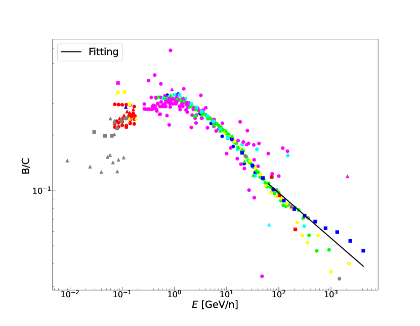
Figure 1: The B/C ratio as a function of energy per nucleon, $E$. Colored symbols indicate the observational data with different experiments. Colored symbols indicate the observational data with different experiments, as shown in Table 1. Black solid line shows the fitting results of the observational data for energies above $60$ GeV/n.

Figure 1 shows all the observational data available for the B/C ratio, as a function of energy per nucleon, $E$, with various colors and symbols indicating the corresponding experiments as shown in Table 1. It is shown that there is a peak at about $1$ GeV/n for B/C ratio, and a power law may be fitted in high energy (Blasi, 2013). One can suggest that CRs are not significantly influenced by solar modulation if their energies are above $10$ GeV/n (e.g., Strauss & Potgieter, 2014; Qin & Shen, 2017). In this work, with energy range from $6\times 10^{1}$ to $4\times 10^{3}$ GeV/n we fit B/C ratio with a power law

$$\left(\frac{B}{C}\right)=k\left(\frac{E}{E_{0}}\right)^{-\psi},$$ (11)

where $E_{0}=1$ GeV/n, and $k$ and $\psi$ are fitting parameters. The solid line in Figure 1 shows the fitting results with parameters $k\approx 0.31$ and $\psi\approx 0.25$. Here, we set the lower limit of the fitting energy range to be $6\times 10^{1}$ GeV/n to align it with the lower limit of the energy range for anisotropy observations.

Figure 2 shows the CR dipole anisotropy amplitude $\delta$ as a function of total energy $E_{\mathrm{tot}}$. The colored symbols indicate the observational data for different experiments, with error bars showing the total experimental errors of the data. The colored symbols indicate the observational data for different experiments, with error bars showing the total experimental errors of the data, as shown in Table 2. The black solid line indicates the modeling results from Equation (10), with B/C ratio from the fitting results Equation (11). Here, we ignore the difference between the total energy and energy per nucleon for CR anisotropy. It is noted that the fitting of the observational data of B/C ratio are in the energy range $6\times 10^{1}-4\times 10^{3}$ GeV/n, but to obtain the modeling results of the dipole anisotropy amplitude, the fitting results of B/C ratio are used in the energy range $6\times 10^{1}-3\times 10^{11}$ GeV. From Figure 2 we can see that, generally, the observational data and modeling results of the dipole anisotropy amplitude have the similar increasing trend with a power law in the whole energy range, $6\times 10^{1}-3\times 10^{11}$ GeV, apart from the two declining regions around $10^{5}$ GeV and $10^{9}$ GeV in observations. Note that the data uncertainty in the ultra-high energy range is more significant.

4 Conclusions and Discussion

In this work, we follow Jokipii (2007) to derive a model of the CR dipole anisotropy amplitude. We use the simple and effective leaky-box model to describe the propagation of CRs. In the model, the galactic disk is assumed to have a radius which is much larger than the half thickness in $z$ direction. In addition, a galactic halo is supposed to be around the galactic disk. The CRs are considered to escape into the intergalactic space in the $z$ (perpendicular) direction with escape time $\tau_{\mathrm{e}}$ with perpendicular diffusion, assuming the perpendicular escape time much smaller than the parallel one. In addition, we assume the dipole anisotropy amplitude characterized by the angular-dependent CR intensity, considering the high-energy CRs slowly escaping from the Galaxy, in the approximation of the Fick’s diffusion law. To estimate the dipole anisotropy amplitude, we also evaluate the CRs escape time using the simplified leaky-box model considering the secondaries of CRs for the inelastic collisions of the primaries. Note that the escape time is assumed to be independent of CR species. Thus, the CR dipole anisotropy amplitude model is obtained with the ratio between the secondary and primary CRs omnidirectional particle distribution function as an input. To get the modeling results of the CR dipole anisotropy amplitude, we fit the B/C ratio with a power law with energy range from $6\times 10^{1}$ to $4\times 10^{3}$ GeV/n. Using the fitting results of the power law B/C ratio, we get the modeling results of the dipole anisotropy amplitude. It is shown that the observational data and modeling results of the dipole anisotropy amplitude have the similar increasing trend with a power law in the whole energy range from $6\times 10^{1}$ to $3\times 10^{11}$ GeV. Therefore, we suggest that the perpendicular diffusion may play a significant role in CR anisotropy in the energy range.

Typically, researchers have employed more complex models that incorporate various effects when studying cosmic-ray anisotropy, and their results can be well-fitted to the observational data of cosmic rays, even to the extent of reproducing some of the finer details. However, their models and the computation are often complex, which also requires various tuning factors to improve the model outcomes. The model we adopt is relatively simple, hence the agreement between our model predictions and observations is only consistent in the broad energy range in terms of general trends, and our model does not agree with the observations in detail, e.g., there are the two declining regions around $10^{5}$ GeV and $10^{9}$ GeV in observations, which are not shown in the modeling results. On the other hand, the simplicity and analytical nature of our model allows for analytical calculations, and there is no need for much tuning factors in our model, which only requires power law fitting of B/C ratio observations and a few basic parameters for the Galaxy, e.g., the half thickness $h$, gas number density $n_{\mathrm{d}}$, of the galactic disk, and the spallation cross-section $\sigma_{\mathrm{C}\mathrel{\mathchoice{\mkern 2.0mu\clipbox{{.50pt}000}{$\displaystyle\vphantom{+}{\shortrightarrow}$}}{\mkern 2.0mu\clipbox{{.50pt}000}{$\textstyle\vphantom{+}{\shortrightarrow}$}}{\mkern 2.0mu\clipbox{{.50pt}000}{$\scriptstyle\vphantom{+}{\shortrightarrow}$}}{\mkern 2.0mu\clipbox{{.50pt}000}{$\scriptscriptstyle\vphantom{+}{\shortrightarrow}$}}}\mathrm{B}}$. In addition, the modeling of the dipole anisotropy amplitude $\delta$ shows to varying with the CRs energy per nucleon, but observational data of $\delta$ vary with the total energy. We ignore the difference between the total energy and the energy per nucleon, considering the fact that the observed CRs are mostly protons. In addition, The fitting of the observational data of B/C ratio are in the energy range from tens of GeV/n to several TeV/n, but to obtain the modeling results of the dipole anisotropy amplitude, the fitting results of B/C ratio are used in the energy range from tens of GeV to hundreds of EeV. These could all introduce differences between modeling results and observations.

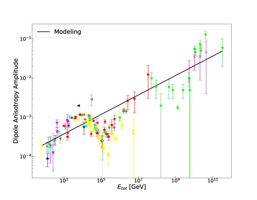
Figure 2: Dipole anisotropy amplitude as a function of total energy, $E_{\mathrm{tot}}$. Colored symbols indicate the observational data with different experiments. Colored symbols indicate the observational data with different experiments, as shown in Table 2. Error bars show the total experimental errors. Black solid line shows the modeling results.

Table 1: Experiments used for B/C data

Experiments	Symbols	Experiments	Symbols	Experiments	Symbols
ACE	${\color[rgb]{1,0,0}\bullet}$	CRN-Spacelab2	${\color[rgb]{1,0,0}\blacksquare}$	ISEE3-HKH	${\color[rgb]{1,0,0}\blacktriangle}$
ASM01	${\color[rgb]{0,0,1}\bullet}$	DAMPE	${\color[rgb]{0,0,1}\blacksquare}$	OGO1	${\color[rgb]{0,0,1}\blacktriangle}$
ASM02	${\color[rgb]{0,1,0}\bullet}$	Gemini11	${\color[rgb]{0,1,0}\blacksquare}$	PAMELA	${\color[rgb]{0,1,0}\blacktriangle}$
ATIC02	${\color[rgb]{0,1,1}\bullet}$	HEAO3-C2	${\color[rgb]{0,1,1}\blacksquare}$	RICH-I	${\color[rgb]{0,1,1}\blacktriangle}$
Balloon	${\color[rgb]{1,0,1}\bullet}$	IMP5	${\color[rgb]{1,0,1}\blacksquare}$	TRACER	${\color[rgb]{1,0,1}\blacktriangle}$
CALET	${\color[rgb]{1,1,0}\bullet}$	IMP7	${\color[rgb]{1,1,0}\blacksquare}$	Ulysses-HET	${\color[rgb]{1,1,0}\blacktriangle}$
CREAM-I	${\color[rgb]{.5,.5,.5}\bullet}$	IMP7	${\color[rgb]{.5,.5,.5}\blacksquare}$	Voyager	${\color[rgb]{.5,.5,.5}\blacktriangle}$

Table 2: Experiments used for the data of dipole anisotropy amplitude

Experiments	Symbols	Experiments	Symbols	Experiments	Symbols
ARGO	${\color[rgb]{1,0,0}\bigstar}$	IceCube	${\color[rgb]{1,1,0}\blacklozenge}$	Mt. Norikura	${\color[rgb]{0,1,1}\blacktriangleleft}$
Artyomovsk	${\color[rgb]{0,0,1}\bigstar}$	IceTop	${\color[rgb]{.5,.5,.5}\blacklozenge}$	Musala	${\color[rgb]{1,0,1}\blacktriangleleft}$
Auger	${\color[rgb]{0,1,0}\bigstar}$	KASCADE	${\color[rgb]{1,0,0}\blacktriangledown}$	Nagoya	${\color[rgb]{1,1,0}\blacktriangleleft}$
Baksan	${\color[rgb]{0,1,1}\bigstar}$	Kamiokande	${\color[rgb]{0,0,1}\blacktriangledown}$	Plateau Rosa	${\color[rgb]{.5,.5,.5}\blacktriangleleft}$
Bolivia	${\color[rgb]{1,0,1}\bigstar}$	LHAASO	${\color[rgb]{0,1,0}\blacktriangledown}$	Poatina	${\color[rgb]{1,0,0}\times}$
Budapest	${\color[rgb]{1,1,0}\bigstar}$	Liapootah	${\color[rgb]{0,1,1}\blacktriangledown}$	Sakashita	${\color[rgb]{0,0,1}\times}$
Carpet	${\color[rgb]{.5,.5,.5}\bigstar}$	London	${\color[rgb]{1,0,1}\blacktriangledown}$	Socorro	${\color[rgb]{0,1,0}\times}$
EAS-TOP	${\color[rgb]{1,0,0}\blacklozenge}$	MACRO	${\color[rgb]{1,1,0}\blacktriangledown}$	Super-Kamiokande	${\color[rgb]{0,1,1}\times}$
EmbudoCave	${\color[rgb]{0,0,1}\blacklozenge}$	Matsushiro	${\color[rgb]{.5,.5,.5}\blacktriangledown}$	Telescope Array	${\color[rgb]{1,0,1}\times}$
HAWC	${\color[rgb]{0,1,0}\blacklozenge}$	Mayflower	${\color[rgb]{1,0,0}\blacktriangleleft}$	Tibet	${\color[rgb]{1,1,0}\times}$
Hobart	${\color[rgb]{0,1,1}\blacklozenge}$	Milagro	${\color[rgb]{0,0,1}\blacktriangleleft}$	Yakutsk	${\color[rgb]{.5,.5,.5}\times}$
Honkong	${\color[rgb]{1,0,1}\blacklozenge}$	Misato	${\color[rgb]{0,1,0}\blacktriangleleft}$

References

- (1)
- (2)
- (3)
- (4)
- (5)
- Berezhko et al. (2003) Berezhko, E. G., Ksenofontov, L. T., Ptuskin, V. S., Zirakashvili, V. N., & Völk, H. J. 2003, A&A, 410, 189
- Berezinskii et al. (1990) Berezinskii, V. S., Bulanov, S. V., Dogiel, V. A., Ginzburg, G. L., & Pstuskin, V. S. 1990, Astrophysics of Cosmic Rays (Amsterdam: North Holland)
- Blasi (2013) Blasi, P. 2013, A&A Rev., 21, 70
- Blasi & Amato (2012) Blasi, P., & Amato, E. 2012, JCAP, 1201, 011
- Cesarsky (1980) Cesarsky, C. J. 1980, ARA&A, 18, 289
- Compton & Getting (1935) Compton, A. H., & Getting, I. A. 1935, PhRv, 47, 817
- Deligny (2016) Deligny, O. 2016, arXiv:1612.08002
- Di Sciascio & Iuppa (2014) Di Sciascio, G., & Iuppa, R. 2014, arXiv:1407.2144
- Erlykin & Wolfendale (2006) Erlykin, A. D., & Wolfendale, A. W. 2006, APh, 25, 183
- Evoli et al. (2012) Evoli, C., Gaggero, D., Grasso, D., & Maccione, L. 2012, PhRvL, 108, 211102
- Génolini et al. (2018) Génolini, Y., Maurin, D., Moskalenko, I. V., & Unger, M. 2018, Phys. Rev. C, 98, 034611
- Gloeckler & Jokipii (1969) Gloeckler, G., & Jokipii, J. R. 1969, Phys. Rev. Lett., 22, 1448
- Jokipii (1966) Jokipii, J. R. 1966, ApJ, 146, 480
- Jokipii (2007) Jokipii, J. R. 2007, New insights into the acceleration and transport of cosmic rays in the galaxy or some simple considerations, presented at the Aspen Workshop on Cosmic-Ray Physics, Aspen, Colorado, April, 18, 2007, https://slideplayer.com/slide/3876575/
- Jones et al. (2001) Jones, F. C., Lukasiak, A., Ptuskin, V., & Webber, W. 2001, ApJ, 547, 264
- Matthaeus et al. (2003) Matthaeus, W. H., Qin, G., Bieber, J. W., & Zank, G. P. 2003, ApJ, 590, L53
- Mertsch & Funk (2015) Mertsch, P., & Funk, S. 2015, Phys. Rev. Lett., 114, 021101
- Pohl & Eichler (2013) Pohl, M., & Eichler, D. 2013, ApJ, 766, 4
- Ptuskin & Soutoul (1990) Ptuskin, V. S., & Soutoul, A. 1990, A&A, 237, 445
- Qiao et al. (2019) Qiao, B.-Q., Liu, W., Guo, Y.-Q., & Yuan, Q. 2019, J. Cosmology Astropart. Phys, 12, 007
- Qin & Shen (2017) Qin, G., & Shen, Z.-N. 2017, ApJ, 846, 56
- Qu et al. (2012) Qu, X.-B., Zhang, Y., Xue, L., Liu, C., & Hu, H.-B. 2012, ApJ, 750, L17
- Reeves et al. (1970) Reeves, H., Fowler, W. A., & Hoyle, F. 1970, Nature, 226, 727
- Schlickeiser et al. (2019) Schlickeiser, R., Oppotsch1, J., Zhang, M., & Pogorelov, N. V. 2019, ApJ, 879, 29
- Strauss & Potgieter (2014) Strauss, R. D., & Potgieter, M. S. 2014, AdSpR, 53, 1015
- Wollan (1939) Wollan, E. O. 1939, RvMP, 11, 160
- Zhang et al. (2014) Zhang, M., Zuo, P.-B, & Pogorelov, N. V. 2014, ApJ, 790, 5
- Zhang et al. (2022) Zhang, Y.-R, Liu, S.-M, & Zeng, H.-D. 2022, MNRAS, 511, 6218
- Zhang et al. (2022) Zhang, Y.-R., Liu, S.-M., & Wu, D.-J. 2022, ApJ, 938, 106
- Zirakashvili (2005) Zirakashvili, V. N. 2005, IJMPA, 20, 6858