A Semi-Empirical Formula for Two-Neutrino Double-Beta Decay

Abstract

We propose a semi-empirical formula for calculating the nuclear matrix elements for two-neutrino double-beta decay. The proposed model (PM) dependence on the proton and neutron numbers, the pairing, isospin, and deformation properties of the initial and final nuclei is inspired by the insights offered by nuclear many-body methods. Compared with the previous phenomenological and nuclear models, the PM yields the best agreement with the experimental data. Its stability and predictive power are cross-validated, and predictions for nuclear systems of experimental interest are provided.

Introduction.—In 1935, about a year after the Fermi weak interaction theory was introduced Fermi (1934), Wigner drew attention to the two-neutrino double-beta decay ($2\nu\beta\beta$-decay):

$$(A,Z)\rightarrow(A,Z+2)+e^{-}+e^{-}+\overline{\nu}_{e}+\overline{\nu}_{e}.$$ (1)

In this process, two neutrons in the nucleus are converted into two protons while emitting two electrons and two electron antineutrinos. Goeppert-Mayer estimated the half-life of $2\nu\beta\beta$-decay to be $10^{17}$ years by assuming a $Q$-value of about 10 MeV Goeppert-Mayer (1935). In 1939, after Majorana formulated the theory of Majorana neutrinos Majorana (1937), Furry proposed the concept of neutrinoless double-beta decay ($0\nu\beta\beta$-decay) Furry (1939),

$$(A,Z)\rightarrow(A,Z+2)+e^{-}+e^{-}.$$ (2)

This process involves two subsequent $\beta$ decays of neutrons connected via the exchange of virtual neutrinos Racah (1937). There are other modes of double-beta decay transforming the $(A,Z+2)$ nucleus into the $(A,Z)$ nucleus Doi and Kotani (1992, 1993): the double-positron emitting ($2\nu/0\nu\beta^{+}\beta^{+}$) mode, the atomic electron capture with coincident positron emission ($2\nu/0\nu\textrm{EC}\beta^{+}$) mode, and the double electron capture ($2\nu/0\nu\textrm{ECEC}$) mode. These processes are less favored due to smaller $Q$-value, small overlap of the bound electron wave function with the nucleus, and Coulomb repulsion on positrons.

The primary focus is on studying $0\nu\beta\beta$-decay, which is not allowed by the Standard Model of particle physics. Thus, it can provide insight into neutrinos’ Majorana nature, masses, and CP properties by violating the total lepton number Schechter and Valle (1982); Sujkowski and Wycech (2004); Pascoli et al. (2006); Bilenky and Giunti (2015); Vergados et al. (2016); Girardi et al. (2016); Šimkovic (2021). To date, the $0\nu\beta\beta$-decay has not been observed. The best lower limit on the half-life of this process is approximately $T_{1/2}^{0\nu}\gtrsim 10^{26}$ years for ⁷⁶Ge Agostini et al. (2020) and ¹³⁶Xe Abe et al. (2023). The discovery of $0\nu\beta\beta$-decay would have far-reaching implications for particle physics and fundamental symmetries.

The first direct observation of $2\nu\beta\beta$-decay, allowed by the SM, was achieved for ⁸²Se in 1987 Elliott et al. (1987); Moe (2014). Nowadays, the $2\nu\beta\beta$-decay has been detected in direct counter experiments in nine different nuclei, including decays into two excited states. In addition to laboratory experiments, geochemical and radiochemical observations of $2\nu\beta\beta$-decay transitions have been recorded Barabash (2020) (and references therein). Furthermore, there are some positive indications of the $2\nu\textrm{ECEC}$ mode for ¹³⁰Ba and ¹³²Ba from geochemical measurements Barabash and Saakyan (1996a); Meshik et al. (2001a); Pujol et al. (2009) and for ⁷⁸Kr Gavrilyuk et al. (2013); Ratkevich et al. (2017a) and, recently, the first direct observation of the $2\nu\textrm{ECEC}$ process in ¹²⁴Xe have been claimed Aprile et al. (2019, 2022a). The measurement of $2\nu\beta\beta$-decay yields valuable insights into nuclear structure physics, which can be used in $0\nu\beta\beta$-decay calculations and the search for new physics beyond the SM.

The inverse $2\nu\beta\beta$-decay half-life is commonly presented as

$$\left(T^{2\nu}_{1/2}\right)^{-1}=\left|M^{2\nu}\right|^{2}\leavevmode\nobreak\ G^{2\nu},$$ (3)

where $G^{2\nu}$ is the phase-space factor (PSF), and

$$M^{2\nu}=g^{2}_{A}M^{2\nu}_{GT}-g_{V}^{2}M^{2\nu}_{F},$$ (4)

is the nuclear matrix element (NME) governing the transition. $g_{A}$ and $g_{V}=1$ are the axial-vector and vector coupling constants, respectively. The impulse approximation for nucleon current and only $s_{1/2}$ wave states of emitted electrons are considered. The Fermi $M_{F}^{2\nu}$ and Gamow-Teller (GT) $M_{GT}^{2\nu}$ matrix elements are governed by the Fermi and GT operators, which are generators of isospin SU(2) and spin-isospin SU(4) symmetries, respectively. The isospin is known to be a good approximation in nuclei. Thus, it is assumed that $M^{2\nu}_{F}$ is negligibly small, and the main contribution is given by $M^{2\nu}_{GT}$, which takes the form

$$M^{2\nu}_{GT}=m_{e}\sum_{n}\frac{M_{n}}{E_{n}-(E_{i}+E_{f})/2},$$ (5)

with

$$M_{n}=\langle 0^{+}_{f}\|\sum_{m}\tau^{-}_{m}\sigma_{m}\|1^{+}_{n}\rangle\langle 1^{+}_{n}\|\sum_{m}\tau^{-}_{m}\sigma_{m}\|0^{+}_{i}\rangle.$$ (6)

Here, $|0^{+}_{i}\rangle$ ($|0^{+}_{f}\rangle$) is the ground state of the initial (final) even-even nuclei with energy $E_{i}$ ($E_{f}$), and the summations run overall $|1^{+}_{n}\rangle$ states the intermediate odd-odd nucleus with energies $E_{n}$ and overall nucleons $m$ inside the nucleus.

The phase-space part of the decay rate can be accurately computed with a relativistic description of the emitted (captured) electrons in a realistic potential of the final (initial) atomic system. The most precise PSFs computed within the self-consistent Dirac-Hartree-Fock-Slater method, including radiative and atomic exchange corrections Niţescu et al. (2023, 2024), are presented in Table 1. On the other hand, the computation of the NMEs is a challenging and long-standing problem in this field. Due to the growing interest in detecting neutrinoless modes, there have been significant reductions in the uncertainties of half-lives for two-neutrino modes (see $T^{2\nu{\rm-exp}}_{1/2}$ form Table 1) and consequently of the experimental NMEs, i.e., $M^{2\nu-\textrm{exp}}=(T^{2\nu{\rm-exp}}_{1/2}G^{2\nu})^{-1/2}$ (see Tables 2 and 3). The spread and structure of the experimental NMEs are still poorly understood. A model that aligns with the current experimental NMEs could provide realistic recommendations for future experiments across the nuclear chart.

Table 1: The decay properties for various $2\nu\beta\beta$-decays (right arrow) and $2\nu\textrm{ECEC}$ processes (left arrow). $T_{f}$ represents the total isospin of the final nucleus. $\Delta_{p}$ and $\Delta_{n}$ denote experimental proton and neutron pairing gaps in units of MeV, respectively. $\beta^{\rm Z,Z+2}$ is the deformation parameter deduced from the corresponding B(E2) transition. $G^{2\nu}$ in $\textrm{yr}^{-1}$ is the most precise PSF computed in this work for $2\nu\beta\beta$ cases and taken from Niţescu et al. (2024a) (⁷⁸Kr, ¹⁰⁶Cd, ¹³⁰Ba, and ¹³²Ba) and Niţescu et al. (2024b) (¹²⁴Xe) for the $2\nu\textrm{ECEC}$ cases. $T_{1/2}^{2\nu{\rm-ph}}$ and $T_{1/2}^{2\nu{\rm-exp}}$ are the half-lives evaluated with the PM and the experimental half-lives with the smallest uncertainties, respectively. The ⁷⁸Kr data are for double electron capture from $K$ orbital. For ¹²⁸Te, the experimental half-life is obtained using the ratio $T^{2\nu{\rm-exp}}_{1/2}(^{130}\textrm{Te})/T^{2\nu{\rm-exp}}_{1/2}(^{128}\textrm{Te})=\left(3.52\pm 0.11\right)\times 10^{-4}$ Bernatowicz et al. (1993). The transitions under the ”Fitted” label are used as input for the PM, while those under the ”Predicted” label are its predictions.

Nuclear transition	$T_{f}$	$\Delta^{\rm Z}_{p}$	$\Delta^{\rm Z}_{n}$	$\Delta^{\rm Z+2}_{p}$	$\Delta^{\rm Z+2}_{n}$	$\beta^{Z}$	$\beta^{Z+2}$	$G^{2\nu}$	$T^{2\nu{\rm-ph}}_{1/2}$	$T^{2\nu{\rm-exp}}_{1/2}$
Fitted
${{}^{48}_{20}{\rm Ca}_{28}}\rightarrow{{}^{48}_{22}{\rm Ti}_{26}}$	2	2.179	1.688	1.896	1.564	0.107	0.262	$1.58\times 10^{-17}$	$1.2\times 10^{20}$	$6.4^{+1.3}_{-1.1}\times 10^{19}$Arnold et al. (2016a)
${{}^{76}_{32}{\rm Ge}_{44}}\rightarrow{{}^{76}_{34}{\rm Se}_{42}}$	4	1.561	1.535	1.751	1.710	0.188	0.219	$5.07\times 10^{-20}$	$1.8\times 10^{21}$	$2.022^{+0.042}_{-0.042}\times 10^{21}$Agostini et al. (2023)
${{}^{82}_{34}{\rm Se}_{48}}\rightarrow{{}^{82}_{36}{\rm Kr}_{46}}$	5	1.401	1.544	1.734	1.644	0.194	0.203	$1.68\times 10^{-18}$	$9.1\times 10^{19}$	$8.69^{+0.10}_{-0.07}\times 10^{19}$Azzolini et al. (2023)
${{}^{96}_{40}{\rm Zr}_{56}}\rightarrow{{}^{96}_{42}{\rm Mo}_{54}}$	6	1.539	0.846	1.528	1.034	0.060	0.172	$7.24\times 10^{-18}$	$3.4\times 10^{19}$	$2.35^{+0.21}_{-0.21}\times 10^{19}$Argyriades et al. (2010)
${{}^{100}_{42}{\rm Mo}_{58}}\rightarrow{{}^{100}_{44}{\rm Ru}_{56}}$	6	1.612	1.358	1.548	1.296	0.231	0.215	$3.47\times 10^{-18}$	$7.2\times 10^{18}$	$7.07^{+0.11}_{-0.11}\times 10^{18}$Augier et al. (2023)
${{}^{116}_{48}{\rm Cd}_{68}}\rightarrow{{}^{116}_{50}{\rm Sn}_{66}}$	8	1.493	1.377	1.763	1.204	0.135	0.112	$2.91\times 10^{-18}$	$2.3\times 10^{19}$	$2.63^{+0.11}_{-0.12}\times 10^{19}$Barabash et al. (2018)
${{}^{130}_{52}{\rm Te}_{78}}\rightarrow{{}^{130}_{54}{\rm Xe}_{76}}$	11	1.104	1.180	1.307	1.248	0.118	0.128	$1.62\times 10^{-18}$	$7.5\times 10^{20}$	$8.76^{+0.17}_{-0.18}\times 10^{20}$Adams et al. (2021, 2023)
${{}^{136}_{54}{\rm Xe}_{82}}\rightarrow{{}^{136}_{56}{\rm Ba}_{80}}$	12	1.009	1.436	1.265	1.031	0.091	0.125	$1.52\times 10^{-18}$	$2.5\times 10^{21}$	$2.17^{+0.06}_{-0.06}\times 10^{21}$Albert et al. (2014)
${{}^{150}_{60}{\rm Nd}_{90}}\rightarrow{{}^{150}_{62}{\rm Sm}_{88}}$	13	1.224	1.046	1.444	1.193	0.285	0.193	$3.85\times 10^{-17}$	$2.5\times 10^{19}$	$9.3^{+0.7}_{-0.6}\times 10^{18}$Arnold et al. (2016b)
${{}^{238}_{92}{\rm U}_{146}}\rightarrow{{}^{238}_{94}{\rm Pu}_{144}}$	25	0.813	0.606	0.662	0.589	0.289	0.285	$1.65\times 10^{-19}$	$9.1\times 10^{21}$	$2.0^{+0.6}_{-0.6}\times 10^{21}$Turkevich et al. (1991)
Predicted
${{}^{110}_{46}{\rm Pd}_{64}}\rightarrow{{}^{110}_{48}{\rm Cd}_{62}}$	7	1.422	1.442	1.479	1.362	0.257	0.172	$1.46\times 10^{-19}$	$3.1\times 10^{20}$	$>10^{18}$Winter (1952)
${{}^{124}_{50}{\rm Sn}_{74}}\rightarrow{{}^{124}_{52}{\rm Te}_{72}}$	10	1.671	1.314	1.248	1.343	0.0952	0.170	$6.00\times 10^{-19}$	$1.9\times 10^{21}$	–
${{}^{128}_{52}{\rm Te}_{76}}\rightarrow{{}^{128}_{54}{\rm Xe}_{74}}$	10	1.129	1.280	1.319	1.265	0.135	0.202	$3.00\times 10^{-22}$	$1.5\times 10^{24}$	$2.49^{+0.09}_{-0.09}\times 10^{24}$
${{}^{134}_{54}{\rm Xe}_{80}}\rightarrow{{}^{134}_{56}{\rm Ba}_{78}}$	11	1.134	1.029	1.329	1.176	0.115	0.163	$2.25\times 10^{-23}$	$4.0\times 10^{25}$	$>2.8\times 10^{22}$Yan et al. (2024)
Fitted
${{}^{78}_{34}{\rm Se}_{44}}\leftarrow{{}^{78}_{36}{\rm Kr}_{42}}$	5	1.442	1.637	1.577	1.691	0.270	0.256	$5.20\times 10^{-22}$	$1.7\times 10^{23}$	$1.9^{+1.3}_{-0.8}\times 10^{22}$Ratkevich et al. (2017b)
${{}^{124}_{52}{\rm Te}_{72}}\leftarrow{{}^{124}_{54}{\rm Xe}_{70}}$	10	1.249	1.344	1.357	1.339	0.170	0.223	$1.83\times 10^{-20}$	$2.0\times 10^{22}$	$1.10^{+0.22}_{-0.22}\times 10^{22}$Aprile et al. (2022b)
Predicted
${{}^{106}_{46}{\rm Pd}_{60}}\leftarrow{{}^{106}_{48}{\rm Cd}_{58}}$	7	1.472	1.401	1.460	1.338	0.162	0.168	$5.54\times 10^{-21}$	$2.1\times 10^{21}$	$>4.7\times 10^{20}$Belli et al. (2020)
${{}^{130}_{54}{\rm Xe}_{76}}\leftarrow{{}^{130}_{56}{\rm Ba}_{74}}$	11	1.308	1.248	1.351	1.298	0.128	0.215	$1.57\times 10^{-20}$	$6.0\times 10^{22}$	$2.2^{+0.5}_{-0.5}\times 10^{21}$Meshik et al. (2001b)
${{}^{132}_{54}{\rm Xe}_{78}}\leftarrow{{}^{132}_{56}{\rm Ba}_{76}}$	12	1.240	1.181	1.390	1.236	0.141	0.185	$4.09\times 10^{-23}$	$1.0\times 10^{26}$	$>2.2\times 10^{21}$Barabash and Saakyan (1996b)

Table 2: The $2\nu\beta\beta$-decay NMEs obtained with the proposed model (PM), the ones from the SSD hypothesis, and the most recent calculations from various nuclear structure models. The ”Fitted” and ”Predicted” nuclei (see caption of Table 1) are delimited by ”$\chi^{2}/N$” displaying the chi-squared divided by the number of available data for each set.

	$M^{2\nu-\textrm{th}}$										$M^{2\nu-{\rm ph}}$
	pn-QRPA	pn-QRPA	IBM	IBM	IBM	NSM	NSM	PHFB	ET		PM	SSD
Nucleus	Pirinen and Suhonen (2015)	Šimkovic et al. (2018)	Nomura (2024)	Nomura (2022)	Barea et al. (2015)	Patel et al. (2024)	Caurier et al. (2012)	Rath et al. (2019)	Coello Pérez et al. (2018)	$M^{2\nu-\textrm{exp}}$		Kotila and Iachello (2012)
48Ca	–	0.016	0.069	0.024	0.045	–	0.039	–	–	$0.0314\pm 0.0030$	0.022	–
76Ge	–	0.063	0.083	0.018	0.085	–	0.097	–	0.085	$0.0987\pm 0.0010$	0.105	–
82Se	–	0.058	0.072	0.024	0.063	0.099	0.105	–	0.156	$0.0828\pm 0.0005$	0.081	–
96Zr	–	0.133	0.058	0.054	0.034	–	–	0.092	–	$0.0770\pm 0.0040$	0.063	–
100Mo	0.105	0.251	0.197	0.157	0.045	–	–	0.164	0.179	$0.2019\pm 0.0016$	0.199	0.174
116Cd	0.112	0.049	0.089	0.069	0.031	–	–	–	0.137	$0.1142\pm 0.0027$	0.120	0.148
130Te	0.057	0.053	0.035	0.010	0.038	0.027	0.036	0.059	0.034	$0.0265\pm 0.0003$	0.028	–
136Xe	0.036	0.030	0.056	0.022	0.032	0.024	0.021	–	–	$0.0174\pm 0.0002$	0.016	–
150Nd	–	–	0.077	0.054	0.017	0.069	–	0.048	–	$0.0527\pm 0.0019$	0.032	0.023
238U	–	–	–	–	0.023	–	–	–	–	$0.0550\pm 0.0110$	0.026	–
$\chi^{2}/N$	5170	2100	2845	2828	1773	470	686	3442	4774	–	30	233
110Pd	0.167	–	–	0.022	0.041	–	–	–	0.211	$<2.61$	0.147	–
124Sn	0.023	–	–	–	0.034	0.037	–	–	–	–	0.029	–
128Te	0.051	0.063	0.022	0.018	0.044	0.013	0.049	0.058	0.050	$0.0366\pm 0.0007$	0.047	0.015
134Xe	0.063	–	–	–	–	–	–	–	–	$<1.25$	0.033	–

Table 3: The $2\nu\beta\beta$-decay NMEs obtained with previous phenomenological models Ren and Ren (2014); Rajan et al. (2018); Pritychenko (2023) compared with those predicted by: (A) $(Z_{f}/N_{f})^{50}T_{f}^{5}$, (B) $(Z_{f}/N_{f})^{46.94}T_{f}^{4.90}$, (C) $(Z_{f}/N_{f})^{46.94}T_{f}^{4.90}\Delta_{\rm pn}^{0.22}$, (D) $(Z_{f}/N_{f})^{48.44}T_{f}^{4.95}\left[\Delta_{\rm pn}/(\beta_{>}-\beta_{<})\right]^{0.21}$ and (PM) $(Z_{f}/N_{f})^{46.94}T_{f}^{4.90}\left[\Delta_{\rm pn}/(1-\beta_{<}/\beta_{>})\right]^{0.22}$. The ”Fitted” and ”Predicted” nuclei (see caption of Table 1) are delimited by ”$\chi^{2}_{\nu}\leavevmode\nobreak\ (\nu)$” displaying the values of reduced chi-squared (number of DOF) for each model. The last column shows the $\chi^{2}_{\nu}$ when a specific nucleus is involved in the LOOCV for PM.

	$M^{2\nu-\textrm{ph}}$
	Previous models			Present models						LOOCV for PM
Nucleus	Ren and Ren (2014)	Rajan et al. (2018)	Pritychenko (2023)	A	B	C	D	PM	$M^{2\nu-\textrm{exp}}$	$\chi^{2}_{\nu}$ (prediction)
48Ca	0.030	0.035	0.037	0.008	0.012	0.020	0.023	0.022	$0.0314\pm 0.0030$	48 (0.022)
78Ge	0.198	0.123	0.410	0.026	0.044	0.068	0.108	0.105	$0.0987\pm 0.0010$	41 (0.107)
82Se	0.095	0.096	0.163	0.015	0.027	0.040	0.080	0.081	$0.0828\pm 0.0005$	35 (0.073)
96Zr	0.060	0.063	0.008	0.027	0.049	0.058	0.068	0.063	$0.0770\pm 0.0040$	48 (0.063)
100Mo	0.073	0.091	0.220	0.045	0.079	0.110	0.197	0.199	$0.2019\pm 0.0016$	47 (0.183)
116Cd	0.071	0.093	0.121	0.031	0.058	0.081	0.129	0.120	$0.1142\pm 0.0027$	49 (0.121)
130Te	0.077	0.068	0.032	0.006	0.014	0.016	0.029	0.028	$0.0265\pm 0.0003$	32 (0.030)
136Xe	0.030	0.055	0.017	0.004	0.010	0.012	0.016	0.016	$0.0174\pm 0.0002$	40 (0.015)
150Nd	0.030	0.061	0.203	0.009	0.021	0.025	0.027	0.032	$0.0527\pm 0.0019$	29 (0.031)
238U	0.024	–	0.046	0.005	0.014	0.010	0.020	0.026	$0.0550\pm 0.0110$	48 (0.026)
$\chi^{2}_{\nu}\leavevmode\nobreak\ (\nu)$	5651 (9)	24981 (2)	17632 (7)	5450 (8)	3171 (8)	2017 (7)	67 (7)	43 (7)
110Pd	0.135	0.160	0.270	0.047	0.084	0.115	0.143	0.147	$<2.61$
124Sn	0.098	–	0.019	0.009	0.018	0.025	0.029	0.029	–
128Te	0.067	–	0.042	0.014	0.030	0.037	0.045	0.047	$0.0366\pm 0.0007$
134Xe	–	–	0.086	0.010	0.022	0.025	0.033	0.033	$<1.25$

Currently, the predictions of the $2\nu\beta\beta$-decay NMEs are based on various nuclear structure models, such as the proton-neutron quasiparticle random phase approximation (pn-QRPA) and its variants Vogel and Zirnbauer (1986); Civitarese et al. (1987); Aunola and Suhonen (1996); Aunola et al. (1996); Suhonen and Civitarese (1998); Stoica and Klapdor-Kleingrothaus (2001, 2003); Šimkovic et al. (2004); Álvarez-Rodríguez et al. (2004); Rodin et al. (2006); Suhonen and Civitarese (2012); Šimkovic et al. (2013); Pirinen and Suhonen (2015); Šimkovic et al. (2018), the nuclear shell model (NSM) Caurier et al. (1996, 2005); Horoi et al. (2007); Caurier et al. (2012); Neacsu and Horoi (2015); Brown et al. (2015); Horoi and Neacsu (2016); Kostensalo and Suhonen (2020); Patel et al. (2024), the interacting boson model (IBM) Barea et al. (2013, 2015); Nomura (2022, 2024), the projected Hartree-Fock-Bogoliubov (PHFB) method Rath et al. (2019), effective theory (ET) Coello Pérez et al. (2018), and others Kotila et al. (2009); Popara et al. (2022), as well as phenomenological models Ren and Ren (2014); Rajan et al. (2018); Pritychenko (2023). Calculating the $2\nu\beta\beta$-decay NMEs in nuclear theory is challenging due to the complex structure of open-shell medium and heavy nuclei, and the need to describe a complete set of intermediate nucleus states. Only two approaches have been used for a long time: the pn-QRPA and the NSM. Although limited to low-lying excitations, the NSM accounts for all possible correlations. To match the $2\nu\beta\beta$-decay data, the Gamow–Teller operator is adjusted (quenched) to fit the results of single $\beta$ decays or charge exchange reactions, and an unquenched $g_{A}$ is assumed Caurier et al. (1996, 2012). The pn-QRPA includes orbitals far from the Fermi surface, considering high-lying excited states (up to 20-30 MeV), but it included fewer correlations. It was found that $M^{2\nu}_{GT}$ and $M^{2\nu}_{F}$ depend sensitively on the isoscalar and isovector particle-particle interactions of nuclear Hamiltonian, respectively Štefánik et al. (2015); Šimkovic et al. (2018). Recent models like the IBM simplify the low-lying states of the nucleus into $L=0$ ($s$ boson) or $L=2$ ($d$ boson) states, focusing on $0^{+}$ and $2^{+}$ neutron pairs converting into two protons. The PHFB formalism obtains nuclear wave functions with good particle number and angular momentum by projecting on axially symmetric intrinsic HFB states. However, it limits the nuclear Hamiltonian to quadrupole interactions. The impact of this simplification on $M^{2\nu}_{GT}$ calculations is not fully understood. Calculating the $2\nu\beta\beta$-decay NMEs remains a complex and ongoing task in nuclear theory.

Phenomenological models aim to simplify the process description. For example, according to Abad et al. (1983, 1984), $2\nu\beta\beta$-decays with a $1^{+}$ ground state of the intermediate nucleus are determined solely by two virtual $\beta$ decay transitions. The first connects the initial nucleus with the $1^{+}$ intermediate ground state, and the second connects this $1^{+}$ state with the final ground state. This assumption is the single-state dominance (SSD) hypothesis. One advantage of SSD is its independence from the nuclear structure model, as $M^{2\nu}$ can be determined from measured $\log ft$ values or charge-changing reactions. However, a recent study on electron energy distributions in $2\nu\beta\beta$-decay of ¹⁰⁰Mo Augier et al. (2023) suggests that transitions through higher-lying states of the intermediate nucleus also play a crucial role, with destructive interference occurring between these contributions to $M^{2\nu}$.

To our knowledge, three other phenomenological models have been proposed for predicting the $2\nu\beta\beta$-decay half-lives or NMEs. One model Ren and Ren (2014) is similar to the Geiger-Nuttall law used for $\alpha$ decay. The other two models Rajan et al. (2018); Pritychenko (2023) suggest that half-lives or NMEs depend on parameters such as the Coulomb energy parameter ($\xi\approx ZA^{-1/3}$), the $Q$-value, and the quadrupole deformation parameter of the initial nucleus. However, it will be shown later that these models could benefit from refinements to better capture the complexity of the problem.

Phenomenological model.—This letter proposes a phenomenological description of the $2\nu\beta\beta$-decay NMEs, motivated by nuclear theory findings. The proposed model (PM) is

$$M^{2\nu{-ph}}=\left(\frac{Z_{f}}{N_{f}}\right)^{\alpha}\left(\frac{\Delta_{\rm pn}}{1-\beta_{<}/\beta_{>}}\right)^{\gamma}\left(T_{f}\right)^{\sigma},$$ (7)

where $Z_{f}$, $N_{f}$, and $T_{f}$ are the proton number, neutron number, and the isospin of the final nuclear ground state, respectively. We note that the ground state of the initial (final) even-even nucleus belongs to the isospin multiplet with $T_{i}=(N-Z)/2$ ($T_{f}=(N-Z-2)/2$) and it is the only state of this nucleus belonging to that multiplet for which the isospin projection equals the total isospin. The dependence of $M^{2\nu}_{GT}$ on the value of the isospin was established in the study performed within an exactly solvable model Štefánik et al. (2015). The $Z/N$ dependence was motivated by observing that the values of $(Z/N)^{50}T^{5}$, displayed in Figure 1 and Table 3, show a spread similar to $M^{2\nu-\textrm{exp}}$. The six largest peaks correspond to the NMEs for the $2\nu\beta\beta$-decay of ⁹⁸Mo, ¹¹⁴Cd, ¹⁰⁴Ru, ⁹⁴Zr, ¹¹⁰Pd, and ¹⁰⁰Mo, in this order. While ¹⁰⁰Mo has the largest measured NMEs, theoretical predictions Nesterenko et al. (2022); Suhonen (2011); Pirinen and Suhonen (2015) suggest that the other cases might have larger NMEs than ¹⁰⁰Mo. Unfortunately, these cases have not yet been measured due to their lower $Q$-values Tretiak and Zdesenko (2002). It seems $(Z/N)^{50}\leavevmode\nobreak\ T^{5}$ form captures this ordering of NMEs and is a solid base for improvements.

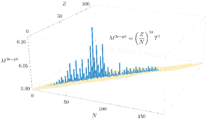
Figure 1: The phenomenological NMEs, obtained using a simplified model $M^{2\nu{-ph}}=(Z/N)^{50}\leavevmode\nobreak\ T^{5}$, are represented in blue in the $(Z,N)$ space for stable even-even nuclei. The base of the representation, shown in orange, corresponds to the known nuclear chart.

Further refinements involve the quantities $\beta_{<}=\min(\beta^{Z},\beta^{Z+2})$ and $\beta_{>}=\max(\beta^{Z},\beta^{Z+2})$, which are defined using $\beta^{Z}$ and $\beta^{Z+2}$, the quadrupole deformation parameters of the initial and final nuclei in their ground states, respectively. This dependence on the deformation parameters reflects the observation from pn-QRPA Šimkovic et al. (2004); Álvarez-Rodríguez et al. (2004), PHFB Chandra et al. (2005); Chaturvedi et al. (2008), and NSM Menéndez et al. (2009) calculations that a mismatch in the deformations of initial and final states reduces the NME value for $2\nu\beta\beta$-decay. Additionally, the pairing parameter $\Delta_{\rm pn}$ is a product of experimental pairing gaps Šimkovic et al. (2003),

$$\Delta_{\rm pn}=\Delta^{\rm Z}_{p}\leavevmode\nobreak\ \Delta^{\rm Z}_{n}\leavevmode\nobreak\ \Delta^{\rm Z+2}_{p}\leavevmode\nobreak\ \Delta^{\rm Z+2}_{n}.$$ (8)

It reflects the significance of transitions through the lowest $1^{+}$ states of the intermediate nucleus. The corresponding $\beta$ transition amplitudes are linked to the BCS $u$ and $v$ occupation amplitudes, which can be derived from the gap parameter.

The best fitting parameters $\alpha$, $\gamma$, and $\sigma$ have been obtained from the minimization of the chi-squared

$$\chi^{2}=\sum_{i=1}^{N}\frac{\left(O_{i}-P_{i}\right)^{2}}{\sigma_{i}^{2}},$$ (9)

where $O_{i}$ is the experimental NME with uncertainty $\sigma_{i}$, and $P_{i}$ is the predicted NME. The sum runs over the direct counter experiments and radiochemical observations. The $2\nu\beta\beta$-decay transitions under the ”Fitted” label from Table 1 ($N=10$), led to the best PM with $\alpha=46.94$, $\gamma=0.22$ and $\sigma=4.90$. Interestingly, when ”Fitted” $2\nu\textrm{ECEC}$ cases were added as inputs ($N=12$), but with $T_{f}\rightarrow T_{f}+1$, the same fit parameters were obtained. This might indicate multilevel modeling for both types of transitions, though more half-life measurements for proton-rich nuclei are needed for a clear answer.

Table 2 compares the $2\nu\beta\beta$-decay NMEs obtained from the PM, the SSD hypothesis, and the most recent calculations of different nuclear models. These datasets are compared using $\chi^{2}/N$ values. The PM shows the best agreement with experimental NMEs, generally yielding $\chi^{2}/N$ values two orders of magnitude smaller than the other calculations. Note that the values for nuclear models in Table 2 are the calculated $M^{2\nu}_{GT}$, each multiplied by the square of an effective $g_{A}$ as chosen by the respective papers. We note smaller $\chi^{2}/N$ values from the SSD hypothesis and NSM calculations, but general conclusions are difficult to draw due to the small number of cases in those datasets. Additionally, we note that the pn-QRPA results from Šimkovic et al. (2018), which include a restoration of the SU(4) symmetry and an effective $g_{A}=0.904$ based on observed $2\nu\beta\beta$-decay half-lives, show a considerable decrease in $\chi^{2}/N$ compared to the pn-QRPA study in Pirinen and Suhonen (2015). In the latter, $\beta$-decay observables adjusted the nucleon-nucleon interaction and single-particle energies for each $\beta\beta$-nuclear system Suhonen (2017).

Table 3 presents the NMEs from present and previous phenomenological models Ren and Ren (2014); Rajan et al. (2018); Pritychenko (2023) alongside the experimental values. To assess the goodness of fit, we computed the reduced chi-squared $\chi^{2}_{\nu}=\chi^{2}/\nu$, where $\nu$ is the number of degrees of freedom (DOF). We note considerably large $\chi^{2}_{\nu}$ values for the previous models. The increase in precision has been introduced gradually from the simplified model A to the PM by varying fit parameters and increasing the model’s complexity (see the caption of Table 3). The best previous model Ren and Ren (2014) is similar in precision to the simplified model A. Our study found that considering the deformation overlap is the most critical refinement of the PM.

We applied leave-one-out cross-validation (LOOCV) to assess the robustness of the PM in describing the experimental data and making predictions. LOOCV involves systematically excluding one data point at a time from the fitting procedure and evaluating the performance of the PM on the remaining data. The values of $\chi^{2}_{\nu}$ for the PM with each exclusion are presented in the last column of Table 3. The NME prediction for the excluded case is presented in parentheses. Excluding a specific case scarcely influences the predictions. Moreover, the small variations in $\chi^{2}_{\nu}$ values confirm the PM’s stability and predictive power.

At first glance, the PM prediction for the $2\nu\beta\beta$-decay NME for ¹²⁸Te seems to disagree with the experimental measurement. However, it should be noted that the latter is obtained from the half-lives ratio of ¹³⁰Te and ¹²⁸Te, derived from geochemical measurements of ancient tellurium ores Bernatowicz et al. (1993). These measurements must be taken with caution, as there might be some unknown production channel of daughter isotopes during their formation. In Dirac (1937); Barabash (1998), it is even suggested that obtained results might be affected by a time dependence of the strength of the weak interaction. These possibilities could also influence the measurements of ¹³⁰Ba and ¹³²Ba. Therefore, we excluded all geochemical cases as inputs from the fit. Only future direct counter experiments on these cases can resolve these ambiguities and confirm the robustness of the PM. Nevertheless, it is interesting to note that the PM predicts quite different NMEs for nuclear systems differing by two neutrons. This is also a feature of the modern nuclear structure models as shown in Table 2 for ¹³⁰Te and ¹²⁸Te. It is also the case of ¹³⁶Xe and its $2\nu\beta\beta$ partner with two neutrons less, ¹³⁴Xe. The prediction of the PM for their NMEs ratio is around $2$, and it might be tested in future liquid Xenon experiments Aprile et al. (2020); Akerib et al. (2020); Aalbers et al. (2016, 2022). Other similar cases are ⁹⁸Mo, ¹¹⁴Cd, and ⁹⁴Zr but their very small $Q$-value limit their near-future measurements.

Conclusions.—In this letter, we proposed a semi-empirical description of the NMEs for two-neutrino double beta decay. Inspired by the findings of nuclear many-body methods, the PM depends on the proton and neutron numbers, pairing, isospin, and deformation properties of the initial and final nuclei. We also found an indication of multilevel modeling for both $2\nu\beta\beta$-decay and $2\nu\textrm{ECEC}$ process, but more measurements for proton-rich nuclei are required for a definitive answer. A comprehensive comparison with previous phenomenological and nuclear models revealed that the PM yields the best agreement with the experimental data, explaining the large spread of measured $2\nu\beta\beta$-decay NMEs. The stability of the PM was confirmed by the LOOCV and reasons to exclude geochemical measurements as inputs were discussed. Finally, we noted that the PM predictions of the NMEs for $2\nu\beta\beta$ nuclear systems differing by two neutrons, are significantly different (by about a factor $2$). Its correctness can be checked by measuring additional $2\nu\beta\beta$ transitions.

Acknowledgments.—O.N. acknowledges support from the Romanian Ministry of Research, Innovation, and Digitalization through Project No. PN 23 08 641 04 04/2023. F.Š. acknowledges support from the Slovak Research and Development Agency under Contract No. APVV-22-0413, VEGA Grant Agency of the Slovak Republic under Contract No. 1/0618/24 and by the Czech Science Foundation (GAČR), project No. 24-10180S.

References

- Fermi (1934) E. Fermi, Zeitschrift für Physik 88, 161 (1934).
- Goeppert-Mayer (1935) M. Goeppert-Mayer, Phys. Rev. 48, 512 (1935).
- Majorana (1937) E. Majorana, Il Nuovo Cimento 14 (1937).
- Furry (1939) W. H. Furry, Phys. Rev. 56, 1184 (1939).
- Racah (1937) G. Racah, Il Nuovo Cimento 14 (1937).
- Doi and Kotani (1992) M. Doi and T. Kotani, Progress of Theoretical Physics 87, 1207 (1992).
- Doi and Kotani (1993) M. Doi and T. Kotani, Progress of Theoretical Physics 89, 139 (1993).
- Schechter and Valle (1982) J. Schechter and J. W. F. Valle, Phys. Rev. D 25, 774 (1982).
- Sujkowski and Wycech (2004) Z. Sujkowski and S. Wycech, Phys. Rev. C 70, 052501 (2004).
- Pascoli et al. (2006) S. Pascoli, S. Petcov, and T. Schwetz, Nuclear Physics B 734, 24 (2006).
- Bilenky and Giunti (2015) S. M. Bilenky and C. Giunti, International Journal of Modern Physics A 30, 1530001 (2015).
- Vergados et al. (2016) J. D. Vergados, H. Ejiri, and F. Šimkovic, International Journal of Modern Physics E 25, 1630007 (2016).
- Girardi et al. (2016) I. Girardi, S. Petcov, and A. Titov, Nuclear Physics B 911, 754 (2016).
- Šimkovic (2021) F. Šimkovic, Physics-Uspekhi 64, 1238 (2021).
- Agostini et al. (2020) M. Agostini, G. R. Araujo, A. M. Bakalyarov, M. Balata, I. Barabanov, L. Baudis, C. Bauer, E. Bellotti, S. Belogurov, A. Bettini, et al. (GERDA Collaboration), Phys. Rev. Lett. 125, 252502 (2020).
- Abe et al. (2023) S. Abe, S. Asami, M. Eizuka, S. Futagi, A. Gando, Y. Gando, T. Gima, A. Goto, T. Hachiya, K. Hata, et al. (KamLAND-Zen Collaboration), Phys. Rev. Lett. 130, 051801 (2023).
- Elliott et al. (1987) S. R. Elliott, A. A. Hahn, and M. K. Moe, Phys. Rev. Lett. 59, 2020 (1987).
- Moe (2014) M. K. Moe, Annual Review of Nuclear and Particle Science 64, 247 (2014).
- Barabash (2020) A. Barabash, Universe 6, 10.3390/universe6100159 (2020).
- Barabash and Saakyan (1996a) A. S. Barabash and R. R. Saakyan, Physics of Atomic Nuclei 59, 179 (1996a).
- Meshik et al. (2001a) A. P. Meshik, C. M. Hohenberg, O. V. Pravdivtseva, and Y. S. Kapusta, Phys. Rev. C 64, 035205 (2001a).
- Pujol et al. (2009) M. Pujol, B. Marty, P. Burnard, and P. Philippot, Geochimica et Cosmochimica Acta 73, 6834 (2009).
- Gavrilyuk et al. (2013) Y. M. Gavrilyuk, A. M. Gangapshev, V. V. Kazalov, V. V. Kuzminov, S. I. Panasenko, and S. S. Ratkevich, Phys. Rev. C 87, 035501 (2013).
- Ratkevich et al. (2017a) S. S. Ratkevich, A. M. Gangapshev, Y. M. Gavrilyuk, F. F. Karpeshin, V. V. Kazalov, V. V. Kuzminov, S. I. Panasenko, M. B. Trzhaskovskaya, and S. P. Yakimenko, Phys. Rev. C 96, 065502 (2017a).
- Aprile et al. (2019) E. Aprile, J. Aalbers, F. Agostini, M. Alfonsi, L. Althueser, F. D. Amaro, et al. (XENON Collaboration), Nature 568, 532 (2019).
- Aprile et al. (2022a) E. Aprile, K. Abe, F. Agostini, S. Ahmed Maouloud, M. Alfonsi, L. Althueser, et al. (XENON Collaboration), Phys. Rev. C 106, 024328 (2022a).
- Niţescu et al. (2023) O. Niţescu, S. Stoica, and F. Šimkovic, Phys. Rev. C 107, 025501 (2023).
- Niţescu et al. (2024) O. Niţescu, R. Dvornický, and F. Šimkovic, Phys. Rev. C 109, 025501 (2024).
- Niţescu et al. (2024a) O. Niţescu, S. Ghinescu, S. Stoica, and F. Šimkovic, Universe 10, 10.3390/universe10020098 (2024a).
- Niţescu et al. (2024b) O. Niţescu, S. Ghinescu, V.-A. Sevestrean, M. Horoi, F. Šimkovic, and S. Stoica, Theoretical analysis and predictions for the double electron capture of 124xe (2024b), arXiv:2402.13784 [nucl-th] .
- Bernatowicz et al. (1993) T. Bernatowicz, J. Brannon, R. Brazzle, R. Cowsik, C. Hohenberg, and F. Podosek, Phys. Rev. C 47, 806 (1993).
- Arnold et al. (2016a) R. Arnold, C. Augier, A. M. Bakalyarov, J. D. Baker, A. S. Barabash, A. Basharina-Freshville, S. Blondel, S. Blot, M. Bongrand, V. Brudanin, et al. (NEMO-3 Collaboration), Phys. Rev. D 93, 112008 (2016a).
- Agostini et al. (2023) M. Agostini, A. Alexander, G. R. Araujo, A. M. Bakalyarov, M. Balata, I. Barabanov, L. Baudis, C. Bauer, S. Belogurov, A. Bettini, et al. (GERDA Collaboration), Phys. Rev. Lett. 131, 142501 (2023).
- Azzolini et al. (2023) O. Azzolini, J. W. Beeman, F. Bellini, M. Beretta, M. Biassoni, C. Brofferio, C. Bucci, S. Capelli, V. Caracciolo, L. Cardani, et al., Phys. Rev. Lett. 131, 222501 (2023).
- Argyriades et al. (2010) J. Argyriades, R. Arnold, C. Augier, J. Baker, A. Barabash, A. Basharina-Freshville, M. Bongrand, G. Broudin-Bay, V. Brudanin, A. Caffrey, et al., Nuclear Physics A 847, 168 (2010).
- Augier et al. (2023) C. Augier, A. S. Barabash, F. Bellini, G. Benato, M. Beretta, L. Bergé, J. Billard, Y. A. Borovlev, L. Cardani, et al. (CUPID-Mo Collaboration), Phys. Rev. Lett. 131, 162501 (2023).
- Barabash et al. (2018) A. S. Barabash, P. Belli, R. Bernabei, F. Cappella, V. Caracciolo, R. Cerulli, D. M. Chernyak, F. A. Danevich, S. d’Angelo, A. Incicchitti, D. V. Kasperovych, V. V. Kobychev, S. I. Konovalov, M. Laubenstein, D. V. Poda, O. G. Polischuk, V. N. Shlegel, V. I. Tretyak, V. I. Umatov, and Y. V. Vasiliev, Phys. Rev. D 98, 092007 (2018).
- Adams et al. (2021) D. Q. Adams, C. Alduino, K. Alfonso, F. T. Avignone, O. Azzolini, G. Bari, F. Bellini, G. Benato, M. Biassoni, A. Branca, et al., Phys. Rev. Lett. 126, 171801 (2021).
- Adams et al. (2023) D. Q. Adams, C. Alduino, K. Alfonso, F. T. Avignone, O. Azzolini, G. Bari, F. Bellini, G. Benato, M. Biassoni, A. Branca, et al., Phys. Rev. Lett. 131, 249902 (2023).
- Albert et al. (2014) J. B. Albert, M. Auger, D. J. Auty, P. S. Barbeau, E. Beauchamp, D. Beck, V. Belov, C. Benitez-Medina, J. Bonatt, M. Breidenbach, et al. (EXO Collaboration), Phys. Rev. C 89, 015502 (2014).
- Arnold et al. (2016b) R. Arnold, C. Augier, J. D. Baker, A. S. Barabash, A. Basharina-Freshville, S. Blondel, S. Blot, M. Bongrand, V. Brudanin, J. Busto, et al. (NEMO-3 Collaboration), Phys. Rev. D 94, 072003 (2016b).
- Turkevich et al. (1991) A. L. Turkevich, T. E. Economou, and G. A. Cowan, Phys. Rev. Lett. 67, 3211 (1991).
- Winter (1952) R. G. Winter, Phys. Rev. 85, 687 (1952).
- Yan et al. (2024) X. Yan, Z. Cheng, A. Abdukerim, Z. Bo, W. Chen, X. Chen, C. Cheng, X. Cui, Y. Fan, D. Fang, et al. (PandaX Collaboration), Phys. Rev. Lett. 132, 152502 (2024).
- Ratkevich et al. (2017b) S. S. Ratkevich, A. M. Gangapshev, Y. M. Gavrilyuk, F. F. Karpeshin, V. V. Kazalov, V. V. Kuzminov, S. I. Panasenko, M. B. Trzhaskovskaya, and S. P. Yakimenko, Phys. Rev. C 96, 065502 (2017b).
- Aprile et al. (2022b) E. Aprile, K. Abe, F. Agostini, S. Ahmed Maouloud, M. Alfonsi, L. Althueser, B. Andrieu, E. Angelino, J. R. Angevaare, V. C. Antochi, et al. (XENON Collaboration), Phys. Rev. C 106, 024328 (2022b).
- Belli et al. (2020) P. Belli, R. Bernabei, V. Brudanin, F. Cappella, V. Caracciolo, R. Cerulli, F. A. Danevich, A. Incicchitti, D. Kasperovych, V. Klavdiienko, V. Kobychev, V. Merlo, O. Polischuk, V. Tretyak, and M. Zarytskyy, Universe 6, 10.3390/universe6100182 (2020).
- Meshik et al. (2001b) A. P. Meshik, C. M. Hohenberg, O. V. Pravdivtseva, and Y. S. Kapusta, Phys. Rev. C 64, 035205 (2001b).
- Barabash and Saakyan (1996b) A. S. Barabash and R. R. Saakyan, Physics of Atomic Nuclei 59, 179 (1996b).
- Pirinen and Suhonen (2015) P. Pirinen and J. Suhonen, Phys. Rev. C 91, 054309 (2015).
- Šimkovic et al. (2018) F. Šimkovic, A. Smetana, and P. Vogel, Phys. Rev. C 98, 064325 (2018).
- Nomura (2024) K. Nomura, Effects of pairing strength on the nuclear structure and double- decay predictions within the mapped interacting boson model (2024), arXiv:2406.02986 [nucl-th] .
- Nomura (2022) K. Nomura, Phys. Rev. C 105, 044301 (2022).
- Barea et al. (2015) J. Barea, J. Kotila, and F. Iachello, Phys. Rev. C 91, 034304 (2015).
- Patel et al. (2024) D. Patel, P. C. Srivastava, V. Kota, and R. Sahu, Nuclear Physics A 1042, 122808 (2024).
- Caurier et al. (2012) E. Caurier, F. Nowacki, and A. Poves, Physics Letters B 711, 62 (2012).
- Rath et al. (2019) P. K. Rath, R. Chandra, K. Chaturvedi, and P. K. Raina, Frontiers in Physics 7, 10.3389/fphy.2019.00064 (2019).
- Coello Pérez et al. (2018) E. A. Coello Pérez, J. Menéndez, and A. Schwenk, Phys. Rev. C 98, 045501 (2018).
- Kotila and Iachello (2012) J. Kotila and F. Iachello, Phys. Rev. C 85, 034316 (2012).
- Ren and Ren (2014) Y. Ren and Z. Ren, Phys. Rev. C 89, 064603 (2014).
- Rajan et al. (2018) M. K. P. Rajan, R. K. Biju, and K. P. Santhosh, Indian Journal of Physics 92, 893 (2018).
- Pritychenko (2023) B. Pritychenko, Nuclear Physics A 1033, 122628 (2023).
- Vogel and Zirnbauer (1986) P. Vogel and M. R. Zirnbauer, Phys. Rev. Lett. 57, 3148 (1986).
- Civitarese et al. (1987) O. Civitarese, A. Faessler, and T. Tomoda, Physics Letters B 194, 11 (1987).
- Aunola and Suhonen (1996) M. Aunola and J. Suhonen, Nuclear Physics A 602, 133 (1996).
- Aunola et al. (1996) M. Aunola, O. Civitarese, J. Kauhanen, and J. Suhonen, Nuclear Physics A 596, 187 (1996).
- Suhonen and Civitarese (1998) J. Suhonen and O. Civitarese, Physics Reports 300, 123 (1998).
- Stoica and Klapdor-Kleingrothaus (2001) S. Stoica and H. Klapdor-Kleingrothaus, Nuclear Physics A 694, 269 (2001).
- Stoica and Klapdor-Kleingrothaus (2003) S. Stoica and H. Klapdor-Kleingrothaus, The European Physical Journal A - Hadrons and Nuclei 17, 529 (2003).
- Šimkovic et al. (2004) F. Šimkovic, L. Pacearescu, and A. Faessler, Nuclear Physics A 733, 321 (2004).
- Álvarez-Rodríguez et al. (2004) R. Álvarez-Rodríguez, P. Sarriguren, E. M. de Guerra, L. Pacearescu, A. Faessler, and F. Šimkovic, Phys. Rev. C 70, 064309 (2004).
- Rodin et al. (2006) V. Rodin, A. Faessler, F. Šimkovic, and P. Vogel, Nuclear Physics A 766, 107 (2006).
- Suhonen and Civitarese (2012) J. Suhonen and O. Civitarese, Journal of Physics G: Nuclear and Particle Physics 39, 085105 (2012).
- Šimkovic et al. (2013) F. Šimkovic, V. Rodin, A. Faessler, and P. Vogel, Phys. Rev. C 87, 045501 (2013).
- Caurier et al. (1996) E. Caurier, F. Nowacki, A. Poves, and J. Retamosa, Phys. Rev. Lett. 77, 1954 (1996).
- Caurier et al. (2005) E. Caurier, G. Martínez-Pinedo, F. Nowacki, A. Poves, and A. P. Zuker, Rev. Mod. Phys. 77, 427 (2005).
- Horoi et al. (2007) M. Horoi, S. Stoica, and B. A. Brown, Phys. Rev. C 75, 034303 (2007).
- Neacsu and Horoi (2015) A. Neacsu and M. Horoi, Phys. Rev. C 91, 024309 (2015).
- Brown et al. (2015) B. A. Brown, D. L. Fang, and M. Horoi, Phys. Rev. C 92, 041301 (2015).
- Horoi and Neacsu (2016) M. Horoi and A. Neacsu, Phys. Rev. C 93, 024308 (2016).
- Kostensalo and Suhonen (2020) J. Kostensalo and J. Suhonen, Physics Letters B 802, 135192 (2020).
- Barea et al. (2013) J. Barea, J. Kotila, and F. Iachello, Phys. Rev. C 87, 014315 (2013).
- Kotila et al. (2009) J. Kotila, J. Suhonen, and D. S. Delion, Journal of Physics G: Nuclear and Particle Physics 37, 015101 (2009).
- Popara et al. (2022) N. Popara, A. Ravlić, and N. Paar, Phys. Rev. C 105, 064315 (2022).
- Štefánik et al. (2015) D. Štefánik, F. Šimkovic, and A. Faessler, Phys. Rev. C 91, 064311 (2015).
- Abad et al. (1983) J. Abad, A. Morales, R. Núñez-Lagos, and A. F. Pacheco, Il Nuovo Cimento A (1965-1970) 75, 173 (1983).
- Abad et al. (1984) J. Abad, A. Morales, R. Núñez-Lagos, and A. Pacheco, Journal de Physique Colloques 45, C3 (1984).
- Nesterenko et al. (2022) D. A. Nesterenko, L. Jokiniemi, J. Kotila, A. Kankainen, Z. Ge, T. Eronen, S. Rinta-Antila, and J. Suhonen, The European Physical Journal A 58, 44 (2022).
- Suhonen (2011) J. Suhonen, Nuclear Physics A 864, 63 (2011).
- Tretiak and Zdesenko (2002) V. I. Tretiak and Y. G. Zdesenko, Atomic Data and Nuclear Data Tables 80, 83 (2002).
- Chandra et al. (2005) R. Chandra, J. Singh, P. K. Rath, P. K. Raina, and J. G. Hirsch, The European Physical Journal A - Hadrons and Nuclei 23, 223 (2005).
- Chaturvedi et al. (2008) K. Chaturvedi, R. Chandra, P. K. Rath, P. K. Raina, and J. G. Hirsch, Phys. Rev. C 78, 054302 (2008).
- Menéndez et al. (2009) J. Menéndez, A. Poves, E. Caurier, and F. Nowacki, Nuclear Physics A 818, 139 (2009).
- Šimkovic et al. (2003) F. Šimkovic, C. C. Moustakidis, L. Pacearescu, and A. Faessler, Phys. Rev. C 68, 054319 (2003).
- Suhonen (2017) J. T. Suhonen, Frontiers in Physics 5, 10.3389/fphy.2017.00055 (2017).
- Dirac (1937) P. A. M. Dirac, Nature 139, 323 (1937).
- Barabash (1998) A. S. Barabash, Journal of Experimental and Theoretical Physics Letters 68, 1 (1998).
- Aprile et al. (2020) E. Aprile et al., Journal of Cosmology and Astroparticle Physics 2020 (11), 031.
- Akerib et al. (2020) D. S. Akerib et al. (LUX-ZEPLIN Collaboration), Phys. Rev. D 101, 052002 (2020).
- Aalbers et al. (2016) J. Aalbers et al., Journal of Cosmology and Astroparticle Physics 2016 (11), 017.
- Aalbers et al. (2022) J. Aalbers et al., Journal of Physics G: Nuclear and Particle Physics 50, 013001 (2022).