Tensor renormalization group study of (1+1)-dimensional U(1) gauge-Higgs model at with Lüscher’s admissibility condition
Abstract
We investigate the phase structure of the (1+1)-dimensional U(1) gauge-Higgs model with a term, where the U(1) gauge action is constructed with Lüscher’s admissibility condition. Using the tensor renormalization group, both the complex action problem and topological freezing problem in the standard Monte Carlo simulation are avoided. We find the first-order phase transition with sufficiently large Higgs mass at , where the charge conjugation symmetry is spontaneously broken. On the other hand, the symmetry is restored with a sufficiently small mass. We determine the critical endpoint as a function of the Higgs mass parameter and show the critical behavior is in the two-dimensional Ising universality class.
1 Introduction
At the end of the last century, Lüscher introduced an admissibility condition for the gauge fields to be separated into disconnected subspaces corresponding to topological charges in the continuum theory Luscher:1998du :
| (1) |
where is a positive constant and is a product of link variables as in the standard way,
| (2) |
The link variable lives on the link connecting the sites and . As an example, he proposed the following gauge action to make the link variables satisfy the above condition:
| (3) |
with the inverse gauge coupling . This action should have an advantage in investigating the topological effects of the gauge theories. However, early numerical studies with this action revealed that the topological change is substantially suppressed in the Monte Carlo histories Fukaya:2003ph and it is difficult to evaluate the contributions from different topological sectors. As long as the Monte Carlo method is employed, the possible way is to perform calculations in the fixed topological sectors Fukaya:2003ph ; Fukaya:2004kp ; Bietenholz:2005rd ; Bietenholz:2016ymo or to utilize open boundary conditions, dismissing the translational invariance of the system Luscher:2011kk .
However, this problem is potentially solved by the tensor renormalization group (TRG) method. 111 In this paper, the “TRG method” or the “TRG approach” refers to not only the original numerical algorithm proposed by Levin and Nave Levin:2006jai but also its extensions Gu:2010yh ; PhysRevB.86.045139 ; Shimizu:2014uva ; Sakai:2017jwp ; Adachi:2019paf ; Kadoh:2019kqk ; Akiyama:2020soe . The major advantages of the TRG method over the Monte Carlo simulation are (i) no sign problem Denbleyker:2013bea ; Shimizu:2014fsa ; Kawauchi:2016xng ; Shimizu:2017onf ; Unmuth-Yockey:2018ugm ; Kadoh:2019ube ; Kuramashi:2019cgs ; Butt:2019uul ; Bloch:2021uup ; Takeda:2021mnc ; Bloch:2021mjw ; Nakayama:2021iyp ; Hirasawa:2021qvh , (ii) logarithmic computational cost on the system size, (iii) direct manipulation of the Grassmann variables Gu:2010yh ; Shimizu:2014uva ; Takeda:2014vwa ; Sakai:2017jwp ; Yoshimura:2017jpk ; Kadoh:2018hqq ; Akiyama:2021xxr ; Bloch:2022vqz ; Akiyama:2023lvr ; Yosprakob:2023tyr ; Asaduzzaman:2023pyz , and (iv) evaluation of the partition function or the path integral itself. The advantage (iv) ensures that the TRG calculation automatically includes full contributions from different topological sectors. Moreover, the TRG method assumes the translational invariance of the system and can easily impose periodic boundary conditions.
In this paper, we investigate the phase structure of the (1+1)-dimensional ((1+1)) U(1) gauge-Higgs model with a term, where the topological effects play an essential role, employing Lüscher’s gauge action of Eq. (3). The Monte Carlo simulation of this model is extremely difficult due to a double whammy of the complex action problem and the topological freezing. Figure 1 illustrates the expected phase diagram Komargodski:2017dmc . The model exhibits the first-order phase transition at , where the charge conjugation symmetry is spontaneously broken in the large positive Higgs mass-squared regime, including the pure gauge limit. 222 There are several earlier studies on the pure gauge theory with a term by the density of state approach Gattringer:2020mbf , complex Langevin method Hirasawa:2020bnl , and TRG Kuramashi:2019cgs ; Hirasawa:2021qvh . Once the Higgs mass-squared is sufficiently reduced, the symmetry is restored. We determine the critical endpoint as a function of the Higgs mass-squared and show its critical behavior is in the 2 Ising universality class based on the numerical analysis of the transfer matrix and topological charge density. We also compare our results with the previous work employing the dual lattice simulation based on the Villain gauge action, which is a non-compact gauge action on the lattice Gattringer:2018dlw .
This paper is organized as follows. In Sec. 2, we define the U(1) gauge-Higgs model with a term on a (1+1) lattice. We also demonstrate how to represent the path integral as a tensor network. In Sec. 3, we first present the results for the pure U(1) gauge action which corresponds to the infinitely heavy limit of the Higgs mass, where the first-order phase transition takes place at . After that, we discuss the phase transition with the finite lattice Higgs mass and determine the critical endpoint and its universality class. Section 4 is devoted to summary and outlook.

2 Tensor network formulation
2.1 The model on a lattice
The U(1) gauge-Higgs model with a term is defined by
| (4) |
We always consider the model on a square lattice with periodic boundary conditions. We employ the Lüscher gauge action,
| (5) |
where is defined by Eq. (2) with and . The admissibility condition is given by
| (6) |
When this condition is satisfied, the corresponding gauge fields are called admissible. The admissibility condition makes gauge fields smooth and unphysical configurations are suppressed. The space of admissible gauge fields is separated into disconnected subspaces which are labeled by the integers corresponding to topological charges in the continuum Luscher:1998du . The Higgs part is defined by
| (7) |
The complex-valued Higgs fields are denoted by and is the lattice Higgs mass where corresponds to the Higgs mass parameter in the continuum action. The quartic coupling constant is denoted by . Finally, the term is defined by
| (8) |
2.2 Tensor network formulation
We consider the tensor network representation of the path integral defined as
| (9) |
Parametrizing the complex-valued Higgs field by , the integral measure is represented as
| (10) |
and reads
| (11) |
We further introduce and rewrite Eq. (11) as
| (12) |
Using the invariance of the Haar measure, or choosing the unitary gauge, we can eliminate from the path integral,
| (13) |
with
| (14) |
In this study, we use the Gauss-Laguerre quadrature rule to discretize the integral over and the Gauss-Legendre one for . The efficacy of these Gauss quadrature rules has been reported in the previous TRG studies for the U(1) pure gauge theory with a term Kuramashi:2019cgs and complex theories Kadoh:2019ube ; Akiyama:2020ntf . The path integral is now approximated by
| (15) |
where
| (16) |
| (17) |
| (18) |
In Eq. (2.2), denotes the sampling point according to the Gauss-Laguerre quadrature and is the corresponding weight. The number of sampling points in is denoted by . Similarly, denotes the sampling point according to the Gauss-Legendre quadrature and is the corresponding weight. The number of sampling points in is denoted by . In the limits of and , the original path integral is restored. Eq. (2.2) is ready to be described as a tensor network. We introduce four-leg pure gauge tensors on each plaquette as follows,
| (19) |
| (20) |
For the Higgs part, we introduce the following hopping matrix,
| (21) |
Now, we perform the singular value decomposition (SVD) of the -directional hopping matrix, which gives us
| (22) |
where and are defined by unitary matrices multiplied by the square root of singular values . In this study, we choose in Eq. (22) such that the singular values satisfying are kept. Note that is the largest singular value and is in the descending order. We are now allowed to integrate out at each site . As a result, we can define a six-leg tensor at each lattice site as,
| (23) |
Therefore, the tensor network representation for Eq. (2.2) is obtained as
| (24) |
with the fundamental tensor at each site ,
| (25) |
whose bond dimension is . Note that the subscripts in the left-hand side of Eq. (25) are defined as with .
2.3 Coarse-graining algorithm
We apply the bond-weighted TRG (BTRG) algorithm PhysRevB.105.L060402 to approximately compute the path integral in Eq. (24). BTRG allows us to approximately carry out the contractions among local tensors within the times of coarse-graining. Since each local tensor in Eq. (25) is defined on each lattice site, relates to the volume via and the linear system size via .
This algorithm improves the accuracy of the original Levin-Nave TRG at the same bond dimension. Remarkably, the computational cost of BTRG is completely the same as the Levin-Nave TRG. The essence of the BTRG is to introduce a weight on each edge of the tensor network. These weights mimic the effect of the environment, which is not taken into account in the original Levin-Nave TRG. Therefore, the BTRG can be regarded as a variant of the second renormalization group algorithms Xie:2009zzd ; PhysRevB.81.174411 . For the algorithmic details, see Ref. PhysRevB.105.L060402 . 333 Since the model is defined on a square lattice, we always set the hyperparameter in the BTRG algorithm as PhysRevB.105.L060402 ; Akiyama:2022pse .
3 Numerical results
In the following, we always set and the positive constant in Eq. (6) as . For the gauge-Higgs model, the quartic coupling is fixed as . Note that the cutoff effects from the finite lattice spacing of the Lüscher gauge action and standard Wilson gauge action are different even at the same inverse gauge coupling . With the same value of , the Lüscher gauge action is expected to be closer to the continuum limit than the Wilson action. See Appendix A for the comparison between the Lüscher and Wilson gauge actions.
3.1 Pure U(1) gauge theory
We start by studying the (1+1) pure gauge theory with a term to validate our tensor network formulation. In this case, the local tensor in Eq. (25) is defined without and the bond dimension in Eq. (24) is equal to .
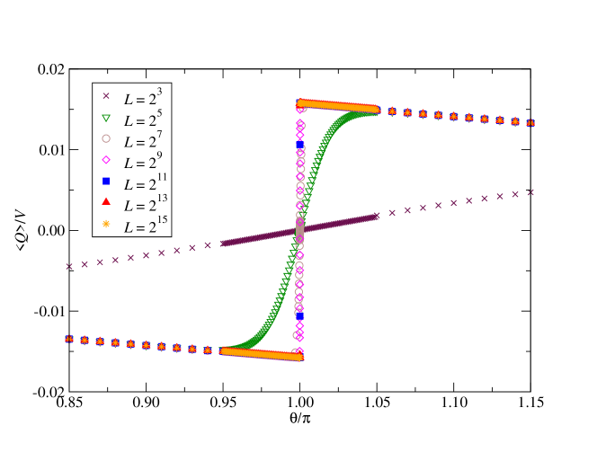
At , the theory is expected to undergo the first-order transition. We calculate the topological charge density , which is defined by
| (26) |
Figure 2 shows the volume dependence of at as a function of . We set and employed the numerical differentiation to evaluate Eq. (26). As the volume increases, the topological charge density gradually becomes discontinuous and we observe a clear jump at with . This is a signal of the first-order transition at .
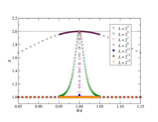
Taking advantage of the TRG method, we also compute the ground state degeneracy by introducing
| (27) |
following Ref. PhysRevB.80.155131 . After sufficient times of coarse-graining, this quantity counts the ground state degeneracy. In Eq. (27), is a transfer matrix defined from the local tensor via
| (28) |
Figure 3 shows in Eq. (27) as a function of . With sufficiently large volume, is realized only at . Therefore, the current TRG computation successfully reproduces the spontaneous symmetry breaking at as expected.
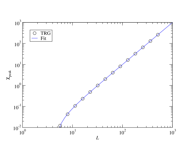
Additionally, we apply the finite-size scaling analysis for the topological susceptibility, which is given by
| (29) |
We use the numerical differentiation with the accuracy, setting around , to evaluate Eq. (29). Since the peak of the topological susceptibility always appears at , we examine the system size dependence of the values of at . Let be the value of at with the linear system size . Using the following ansatz,
| (30) |
the data of are fitted as shown in Figure 4. The fit is performed on the data over and we obtain , , and . Therefore, is proportional to the volume and this is another indication of the first-order phase transition. Although we employed the finite bond dimension and cutoff , the current computation correctly reproduces the first-order phase transition at . We have also tried the same analysis with , which results in , , and . Therefore, seems sufficiently large to investigate the phase transition at for the pure U(1) gauge theory at .
3.2 The U(1) gauge-Higgs model
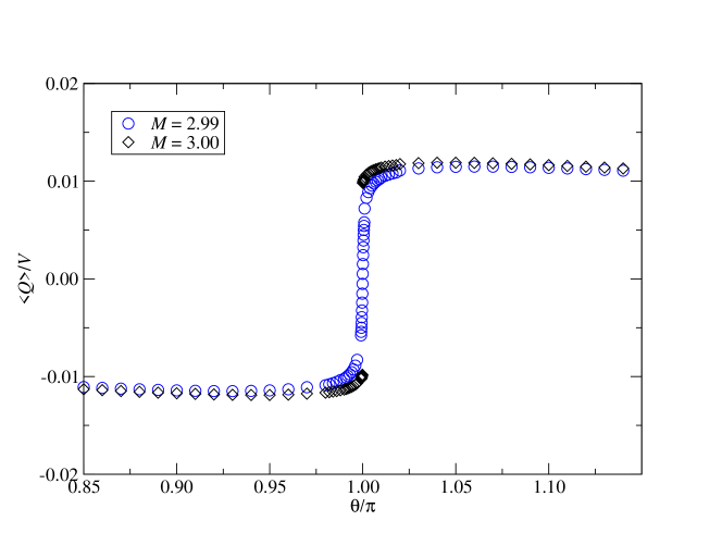
We now investigate the critical behavior of the U(1) gauge-Higgs model at . Figure 5 shows the thermodynamic topological charge density at and , where we set , which result in according to Eq. (22). We also set . As we will see, our choice of is sufficiently large to determine the universality class at the critical endpoint. The behavior of topological charge density is highly different between these two mass parameters; varies continuously around at but the discontinuity appears at when . Therefore, the critical mass should exist in the range of .
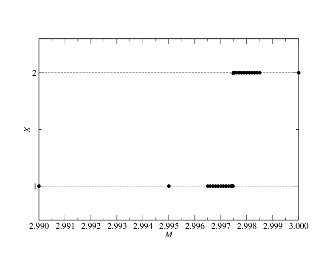
To locate the critical point more precisely, we use the ground state degeneracy in Eq. (27). When , we should have due to the charge symmetry breaking and with , we must have . Figure 6 shows the degeneracy as a function of , which results in .
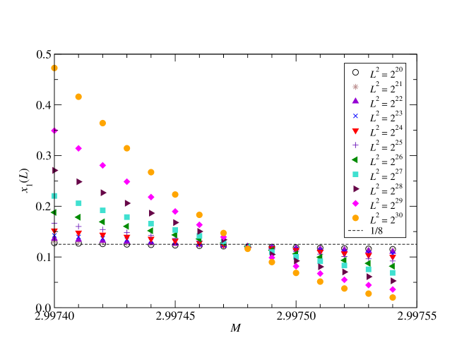
To identify the universality class, we analyze the eigenvalue spectrum of the transfer matrix defined in Eq. (28). Note that the analysis on the transfer matrix obtained from the TRG has been employed in investigating several spin models PhysRevB.104.165132 ; PhysRevB.80.155131 ; Huang:2023vwp ; PhysRevB.108.024413 ; Az-zahra:2024gqr and the lattice Schwinger model Shimizu:2017onf . For a comprehensive overview, see Ref. ueda2024renormalizationgroupflowfixedpoint . Although we are dealing with continuous gauge and scalar degrees of freedom, a similar analysis should be possible if our discretization scheme based on the Gauss quadrature rules is working. Particularly, we employ the tensor-network-based level spectroscopy proposed in Refs. PhysRevB.104.165132 ; PhysRevB.108.024413 . Let be an -th eigenvalue of the transfer matrix . Assuming that these eigenvalues are in descending order, we can obtain the scaling dimension at the finite system size via
| (31) |
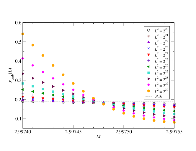
When these quantities are computed at the criticality and on a sufficiently large volume, they give us the scaling dimension of the conformal field theory (CFT). Figure 7 shows as a function of the Higgs mass . The volume independence can be observed at with , which is consistent with the 2 Ising universality class. From now on, we assume the critical phenomenon is in the 2 Ising universality class. Following Ref. PhysRevB.108.024413 , we consider a combined scaling dimension,
| (32) |
which removes the effect of the leading irrelevant perturbation associated with the scaling dimension 4. Since in the 2 Ising universality class, is expected at the criticality. Figure 8 shows against the Higgs mass which is in agreement with this expectation. Note that shown in Figure 8 also agrees with the previous estimation by : . Moreover, we apply a scheme to determine the critical point following Ref. PhysRevB.108.024413 , which assumes the phase transition is in the Ising universality class. We first choose two mass parameters and such that and compute . When (), should increase (decrease) by enlarging the system size as shown in Fig. 8. Secondly, we perform linear interpolations of between and , and find a crossing point of two lines with the system size and . Then, is obtained via , where and are the parameters determined by the numerical fit. The fit results in , where we set , using the data with . Therefore, the tensor-network-based level spectroscopy confirms the critical point estimated by the ground state degeneracy. We also investigate the finite-size correction for the free energy in the thermodynamic limit via
| (33) |
where is the thermodynamic free energy and is the central charge of the CFT at criticality. Using Eq. (33) as a fitting ansatz for , we can determine the central charge. As a representative point, we choose and the fit using the data with results in , which is consistent with , as expected.
We finally remark on the location of which slightly depends on the algorithmic parameters, , , and . Table 1 shows the critical endpoint estimated by the scheme in Ref. PhysRevB.108.024413 . In Table 1, the error originates from the fit based on . We find that these estimations are comparable with obtained in Ref. Gattringer:2018dlw , where the gauge-field Boltzmann weight is given by the Villain form and the Monte Carlo simulation is performed based on the dual representation. Note that in Ref. Gattringer:2018dlw is obtained at and .
| 24 | 20 | 8 | 192 | 2.9982886(1) |
| 22 | 20 | 8 | 176 | 2.9998263(13) |
| 20 | 20 | 8 | 160 | 2.9974765(14) |
| 24 | 10 | 6 | 144 | 2.9929635(1) |
| 22 | 10 | 6 | 132 | 2.9945222(9) |
| 20 | 10 | 7 | 140 | 2.9921698(6) |
4 Summary and outlook
We have analyzed the phase structure of the (1+1) U(1) gauge-Higgs model with a term, whose gauge action is constructed with Lüscher’s admissibility condition. Although the model suffers from a complex action problem and topological freezing within the Monte Carlo simulation, the TRG approach allows us to deal with the model successfully. We have observed the first-order phase transition at with sufficiently large lattice Higgs mass , including the pure gauge theory, with the finite gauge coupling and the quartic coupling . We have determined the critical endpoint and its universality class from the numerical analysis of the transfer matrix, which can be directly obtained from the TRG computation. Employing the tensor-network-based level spectroscopy, we have confirmed that the scaling dimensions are consistent with the 2 Ising universality class.
All these results show that the TRG is a promising approach to deal with the lattice gauge theory with Lüscher’s admissibility condition. We emphasize that one can easily combine the Lüscher gauge action with fermions and extend the theory for the higher dimensions within the tensor network formulation. It would be an interesting future work to investigate the Schwinger model with a term under Lüscher’s admissibility condition.
Acknowledgements.
Numerical calculation for the present work was carried out with SQUID at the Cybermedia Center, Osaka University (Project ID: hp240012). We also used the supercomputer Fugaku provided by RIKEN through the HPCI System Research Project (Project ID: hp230247) and computational resources of Wisteria/BDEC-01 and Cygnus and Pegasus under the Multidisciplinary Cooperative Research Program of Center for Computational Sciences, University of Tsukuba. This work is supported by Grants-in-Aid for Scientific Research from the Ministry of Education, Culture, Sports, Science and Technology (MEXT) (Nos. 24H00214, 24H00940). SA acknowledges the support from the Endowed Project for Quantum Software Research and Education, the University of Tokyo qsw , JSPS KAKENHI Grant Number JP23K13096, and the Center of Innovations for Sustainable Quantum AI (JST Grant Number JPMJPF2221).Appendix A Comparison with the Wilson gauge action
Employing the pure U(1) gauge theory with a term, we make a comparison between the Lüscher gauge action in Eq. (5) and the Wilson gauge action,
| (34) |
Here, we consider a term defined by
| (35) |
instead of Eq. (8). In the continuum limit, Eq. (35) reproduces
| (36) |
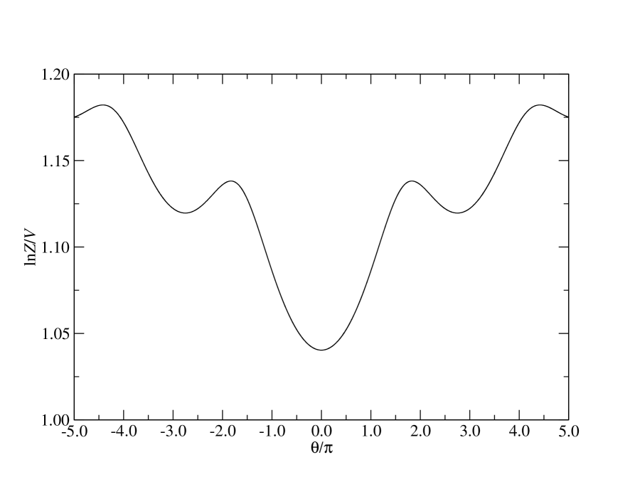
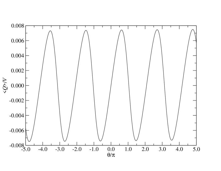
which is a topological term of the continuum theory and is the field strength in two dimensions. The continuum limit is defined by and with fixing . The term in Eq. (35) reproduces the periodicity of observables as a function of with sufficiently large and Gattringer:2015baa .
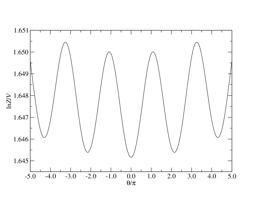
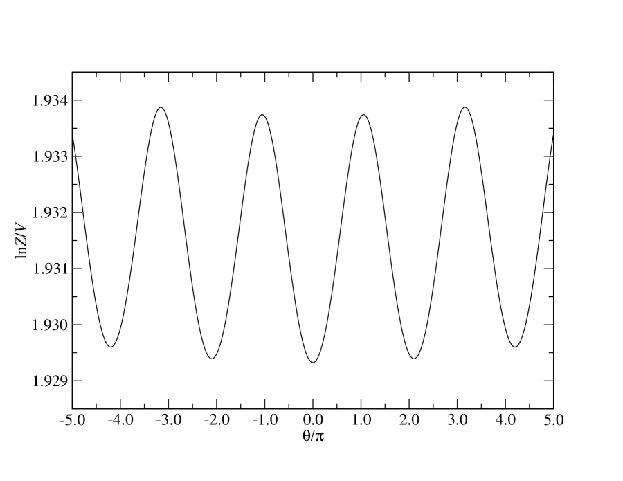
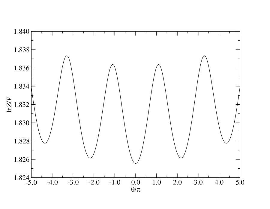
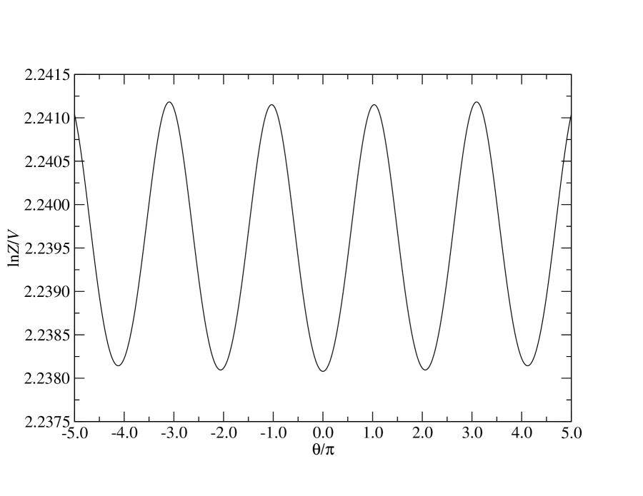
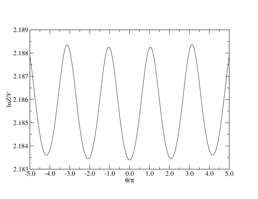
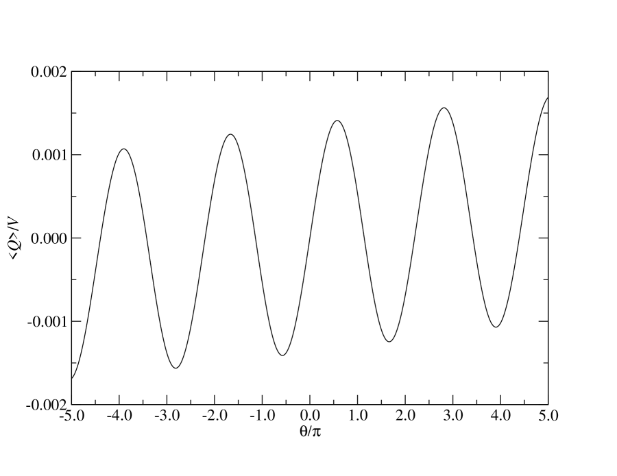
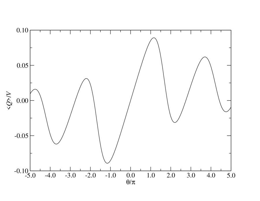
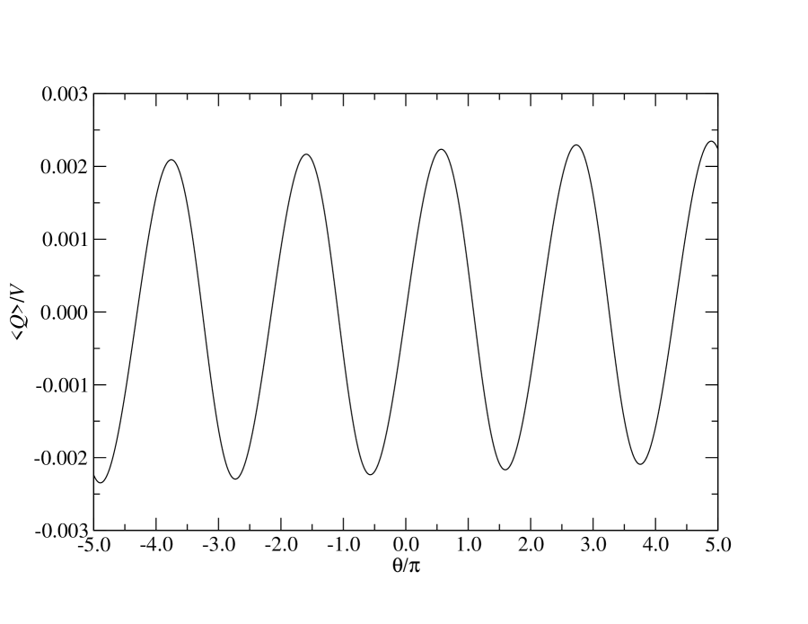
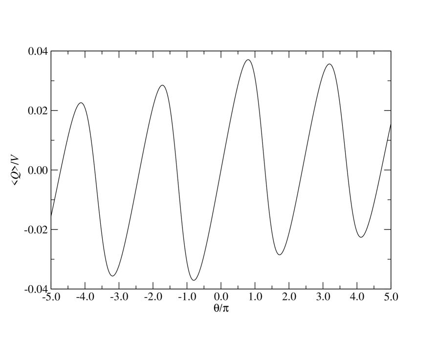
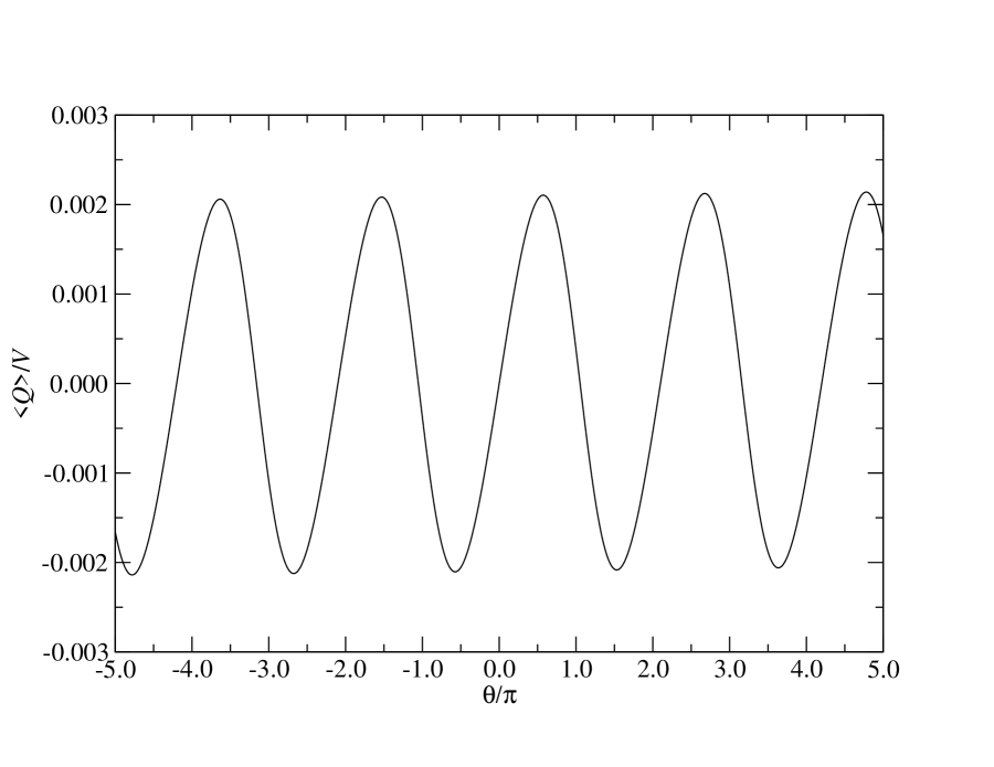
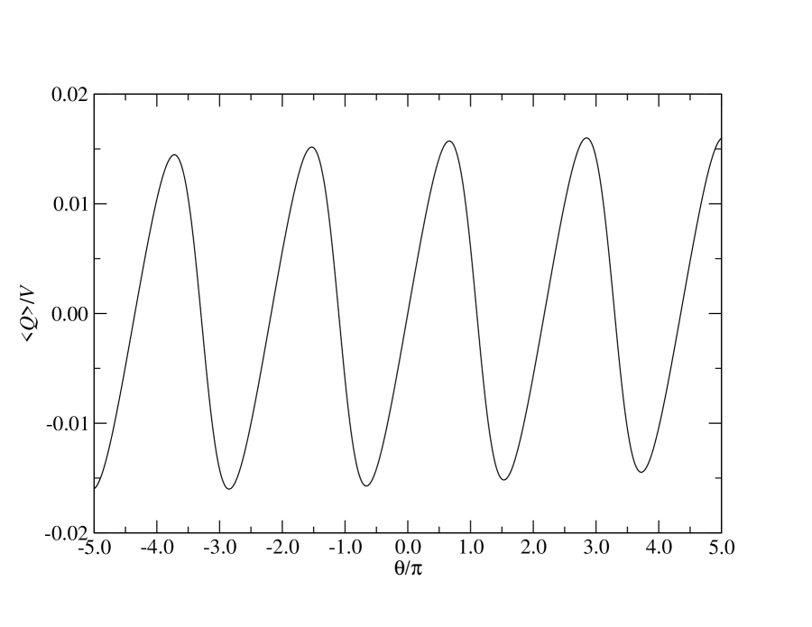
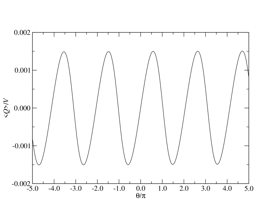
Since the cutoff effects in the Lüscher and Wilson gauge actions should differ, how to approach the continuum limit should also be different. In Figure 9, the free energy density is shown as a function of at various with fixing . All these results are obtained by the BTRG with . The left and right panels are obtained by the Lüscher action with and Wilson action at the same and . Figure 10 shows the topological charge density defined by Eq. (26) in the same way. With the same , the Lüscher action gives a result closer to the continuum limit than the Wilson action.
For more quantitative discussion, we compute the topological susceptibility given by Eq. (29) employing the numerical differentiation with the accuracy, setting . In particular, we investigate the peak position of varying and with fixing , fitting via three parameters , , and by
| (37) |
in the vicinity of the first peak appearing in the region where is positive. Typically, we use 2000 data points around . Table 2 summarizes the resulting peak position in the unit of . At the same , the Lüscher action results in the peak position closer to than the Wilson action. Since we should observe the peaks in the topological susceptibility at in the limits of and , we can conclude that the Lüscher gauge action shows a faster convergence toward the continuum limit than the Wilson gauge action.
(a)

 (b)
(b)
 (c)
(c)
 (d)
(d)
(a)
 (b)
(b)
 (c)
(c)
 (d)
(d)
| Lüscher () | Wilson | |
|---|---|---|
| 1.67903(2) | ||
| 1.26026(1) | ||
| 1.09604(7) | ||
| 1.04296(1) |
References
- (1) M. Lüscher, Abelian chiral gauge theories on the lattice with exact gauge invariance, Nucl. Phys. B 549 (1999) 295–334, [hep-lat/9811032].
- (2) H. Fukaya and T. Onogi, Lattice study of the massive Schwinger model with theta term under Lüscher’s “admissibility” condition, Phys. Rev. D 68 (2003) 074503, [hep-lat/0305004].
- (3) H. Fukaya and T. Onogi, Theta vacuum effects on the chiral condensation and the eta-prime meson correlators in the two flavor massive QED(2) on the lattice, Phys. Rev. D 70 (2004) 054508, [hep-lat/0403024].
- (4) W. Bietenholz, K. Jansen, K. I. Nagai, S. Necco, L. Scorzato and S. Shcheredin, Exploring topology conserving gauge actions for lattice QCD, JHEP 03 (2006) 017, [hep-lat/0511016].
- (5) W. Bietenholz, C. Czaban, A. Dromard, U. Gerber, C. P. Hofmann, H. Mejía-Díaz et al., Interpreting Numerical Measurements in Fixed Topological Sectors, Phys. Rev. D 93 (2016) 114516, [1603.05630].
- (6) M. Lüscher and S. Schaefer, Lattice QCD without topology barriers, JHEP 07 (2011) 036, [1105.4749].
- (7) M. Levin and C. P. Nave, Tensor renormalization group approach to two-dimensional classical lattice models, Phys. Rev. Lett. 99 (2007) 120601, [cond-mat/0611687].
- (8) Z.-C. Gu, F. Verstraete and X.-G. Wen, Grassmann tensor network states and its renormalization for strongly correlated fermionic and bosonic states, 1004.2563.
- (9) Z. Y. Xie, J. Chen, M. P. Qin, J. W. Zhu, L. P. Yang and T. Xiang, Coarse-graining renormalization by higher-order singular value decomposition, Phys. Rev. B 86 (Jul, 2012) 045139, [1201.1144].
- (10) Y. Shimizu and Y. Kuramashi, Grassmann tensor renormalization group approach to one-flavor lattice Schwinger model, Phys. Rev. D90 (2014) 014508, [1403.0642].
- (11) R. Sakai, S. Takeda and Y. Yoshimura, Higher order tensor renormalization group for relativistic fermion systems, PTEP 2017 (2017) 063B07, [1705.07764].
- (12) D. Adachi, T. Okubo and S. Todo, Anisotropic Tensor Renormalization Group, Phys. Rev. B 102 (2020) 054432, [1906.02007].
- (13) D. Kadoh and K. Nakayama, Renormalization group on a triad network, 1912.02414.
- (14) S. Akiyama, Y. Kuramashi, T. Yamashita and Y. Yoshimura, Restoration of chiral symmetry in cold and dense Nambu–Jona-Lasinio model with tensor renormalization group, JHEP 01 (2021) 121, [2009.11583].
- (15) A. Denbleyker, Y. Liu, Y. Meurice, M. P. Qin, T. Xiang, Z. Y. Xie et al., Controlling Sign Problems in Spin Models Using Tensor Renormalization, Phys. Rev. D89 (2014) 016008, [1309.6623].
- (16) Y. Shimizu and Y. Kuramashi, Critical behavior of the lattice Schwinger model with a topological term at using the Grassmann tensor renormalization group, Phys. Rev. D90 (2014) 074503, [1408.0897].
- (17) H. Kawauchi and S. Takeda, Tensor renormalization group analysis of CP(-1) model, Phys. Rev. D93 (2016) 114503, [1603.09455].
- (18) Y. Shimizu and Y. Kuramashi, Berezinskii-Kosterlitz-Thouless transition in lattice Schwinger model with one flavor of Wilson fermion, Phys. Rev. D97 (2018) 034502, [1712.07808].
- (19) J. Unmuth-Yockey, J. Zhang, A. Bazavov, Y. Meurice and S.-W. Tsai, Universal features of the Abelian Polyakov loop in 1+1 dimensions, Phys. Rev. D98 (2018) 094511, [1807.09186].
- (20) D. Kadoh, Y. Kuramashi, Y. Nakamura, R. Sakai, S. Takeda and Y. Yoshimura, Investigation of complex theory at finite density in two dimensions using TRG, JHEP 02 (2020) 161, [1912.13092].
- (21) Y. Kuramashi and Y. Yoshimura, Tensor renormalization group study of two-dimensional U(1) lattice gauge theory with a term, JHEP 04 (2020) 089, [1911.06480].
- (22) N. Butt, S. Catterall, Y. Meurice, R. Sakai and J. Unmuth-Yockey, Tensor network formulation of the massless Schwinger model with staggered fermions, Phys. Rev. D 101 (2020) 094509, [1911.01285].
- (23) J. Bloch, R. Lohmayer, S. Schweiss and J. Unmuth-Yockey, Effective model for finite-density QCD with tensor networks, 10, 2021, 2110.09499.
- (24) S. Takeda, A novel method to evaluate real-time path integral for scalar theory, PoS LATTICE2021 (2022) 532, [2108.10017].
- (25) J. Bloch, R. G. Jha, R. Lohmayer and M. Meister, Tensor renormalization group study of the three-dimensional O(2) model, Phys. Rev. D 104 (2021) 094517, [2105.08066].
- (26) K. Nakayama, L. Funcke, K. Jansen, Y.-J. Kao and S. Kühn, Phase structure of the CP(1) model in the presence of a topological -term, Phys. Rev. D 105 (2022) 054507, [2107.14220].
- (27) M. Hirasawa, A. Matsumoto, J. Nishimura and A. Yosprakob, Tensor renormalization group and the volume independence in 2D U(N) and SU(N) gauge theories, JHEP 12 (2021) 011, [2110.05800].
- (28) S. Takeda and Y. Yoshimura, Grassmann tensor renormalization group for the one-flavor lattice Gross-Neveu model with finite chemical potential, PTEP 2015 (2015) 043B01, [1412.7855].
- (29) Y. Yoshimura, Y. Kuramashi, Y. Nakamura, S. Takeda and R. Sakai, Calculation of fermionic Green functions with Grassmann higher-order tensor renormalization group, Phys. Rev. D97 (2018) 054511, [1711.08121].
- (30) D. Kadoh, Y. Kuramashi, Y. Nakamura, R. Sakai, S. Takeda and Y. Yoshimura, Tensor network formulation for two-dimensional lattice = 1 Wess-Zumino model, JHEP 03 (2018) 141, [1801.04183].
- (31) S. Akiyama and Y. Kuramashi, Tensor renormalization group approach to (1+1)-dimensional Hubbard model, Phys. Rev. D 104 (2021) 014504, [2105.00372].
- (32) J. Bloch and R. Lohmayer, Grassmann higher-order tensor renormalization group approach for two-dimensional strong-coupling QCD, Nucl. Phys. B 986 (2023) 116032, [2206.00545].
- (33) S. Akiyama, Matrix product decomposition for two- and three-flavor Wilson fermions: Benchmark results in the lattice Gross-Neveu model at finite density, Phys. Rev. D 108 (2023) 034514, [2304.01473].
- (34) A. Yosprakob, J. Nishimura and K. Okunishi, A new technique to incorporate multiple fermion flavors in tensor renormalization group method for lattice gauge theories, JHEP 11 (2023) 187, [2309.01422].
- (35) M. Asaduzzaman, S. Catterall, Y. Meurice, R. Sakai and G. C. Toga, Tensor network representation of non-abelian gauge theory coupled to reduced staggered fermions, JHEP 05 (2024) 195, [2312.16167].
- (36) Z. Komargodski, A. Sharon, R. Thorngren and X. Zhou, Comments on Abelian Higgs Models and Persistent Order, SciPost Phys. 6 (2019) 003, [1705.04786].
- (37) C. Gattringer and O. Orasch, Density of states approach for lattice gauge theory with a -term, Nucl. Phys. B 957 (2020) 115097, [2004.03837].
- (38) M. Hirasawa, A. Matsumoto, J. Nishimura and A. Yosprakob, Complex Langevin analysis of 2D U(1) gauge theory on a torus with a term, JHEP 09 (2020) 023, [2004.13982].
- (39) C. Gattringer, D. Göschl and T. Sulejmanpasic, Dual simulation of the 2d U(1) gauge Higgs model at topological angle : Critical endpoint behavior, Nucl. Phys. B 935 (2018) 344–364, [1807.07793].
- (40) S. Akiyama, D. Kadoh, Y. Kuramashi, T. Yamashita and Y. Yoshimura, Tensor renormalization group approach to four-dimensional complex theory at finite density, JHEP 09 (2020) 177, [2005.04645].
- (41) D. Adachi, T. Okubo and S. Todo, Bond-weighted tensor renormalization group, Phys. Rev. B 105 (Feb, 2022) L060402, [2011.01679].
- (42) Z. Y. Xie, H. C. Jiang, Q. N. Chen, Z. Y. Weng and T. Xiang, Second Renormalization of Tensor-Network States, Phys. Rev. Lett. 103 (2009) 160601, [0809.0182].
- (43) H. H. Zhao, Z. Y. Xie, Q. N. Chen, Z. C. Wei, J. W. Cai and T. Xiang, Renormalization of tensor-network states, Phys. Rev. B 81 (May, 2010) 174411.
- (44) S. Akiyama, Bond-weighting method for the Grassmann tensor renormalization group, JHEP 11 (2022) 030, [2208.03227].
- (45) Z.-C. Gu and X.-G. Wen, Tensor-entanglement-filtering renormalization approach and symmetry-protected topological order, Phys. Rev. B 80 (Oct, 2009) 155131.
- (46) A. Ueda and M. Oshikawa, Resolving the berezinskii-kosterlitz-thouless transition in the two-dimensional xy model with tensor-network-based level spectroscopy, Phys. Rev. B 104 (Oct, 2021) 165132.
- (47) C.-Y. Huang, S.-H. Chan, Y.-J. Kao and P. Chen, Tensor network based finite-size scaling for two-dimensional Ising model, Phys. Rev. B 107 (2023) 205123, [2302.02585].
- (48) A. Ueda and M. Oshikawa, Finite-size and finite bond dimension effects of tensor network renormalization, Phys. Rev. B 108 (Jul, 2023) 024413.
- (49) F. I. Az-zahra, S. Takeda and T. Yamazaki, Spectroscopy by Tensor Renormalization Group Method, 2404.15666.
- (50) A. Ueda, Renormalization group flow and fixed-point in tensor network representations, 2024.
- (51) https://qsw.phys.s.u-tokyo.ac.jp/.
- (52) C. Gattringer, T. Kloiber and M. Müller-Preussker, Dual simulation of the two-dimensional lattice U(1) gauge-Higgs model with a topological term, Phys. Rev. D 92 (2015) 114508, [1508.00681].