Communication- and Computation-Efficient Distributed Decision-Making in Multi-Robot Networks

Abstract

We provide a distributed coordination paradigm that enables scalable and near-optimal joint motion planning among multiple robots. Our coordination paradigm is in contrast to the current paradigms that are either near-optimal but impractical for replanning times or real-time but offer no near-optimality guarantees. We are motivated by the future of collaborative mobile autonomy where distributed teams of robots will be coordinating via vehicle-to-vehicle (v2v) communication to execute information-heavy tasks such as mapping, surveillance, and target tracking. To enable rapid distributed coordination, we need to curtail the explosion of information-sharing across the network, thus, we need to limit how much the robots coordinate. However, limiting coordination can lead to suboptimal joint plans, causing non-coordinating robots to execute overlapping trajectories, instead of complementary. In this paper, we make theoretical and algorithmic contributions to characterize and balance this trade-off between decision speed and optimality. To this end, we introduce tools for distributed submodular optimization. Submodularity is a diminishing returns property typically arising in information-gathering tasks such as the aforementioned ones. On the theoretical side, we provide an analysis of how the network topology at the local level —each robot’s local coordination neighborhood— affects the near-optimality of coordination at the global level. On the algorithmic side, we provide a communication- and computation-efficient coordination algorithm that enables the agents to individually balance the trade-off. Our algorithm is up to two orders faster than competitive near-optimal algorithms. In simulations of surveillance tasks with up to 45 robots, the algorithm enables real-time planning at the order of $1$ Hz with superior coverage performance. To enable the simulations, we provide a high-fidelity simulator that extends AirSim by integrating a collaborative autonomy pipeline and simulating v2v communication delays.

I Introduction

In the future, distributed teams of robots will be coordinating via robot-to-robot communication to execute tasks such as collaborative mapping [1], surveillance [2], and target tracking [3] (Fig. 1). To this end, the robots will be adapting the information flow in the team to enable rapid and optimal decision-making (Fig. 2). Specifically, subject to their computation  and  communication bandwidth constraints,  the robots

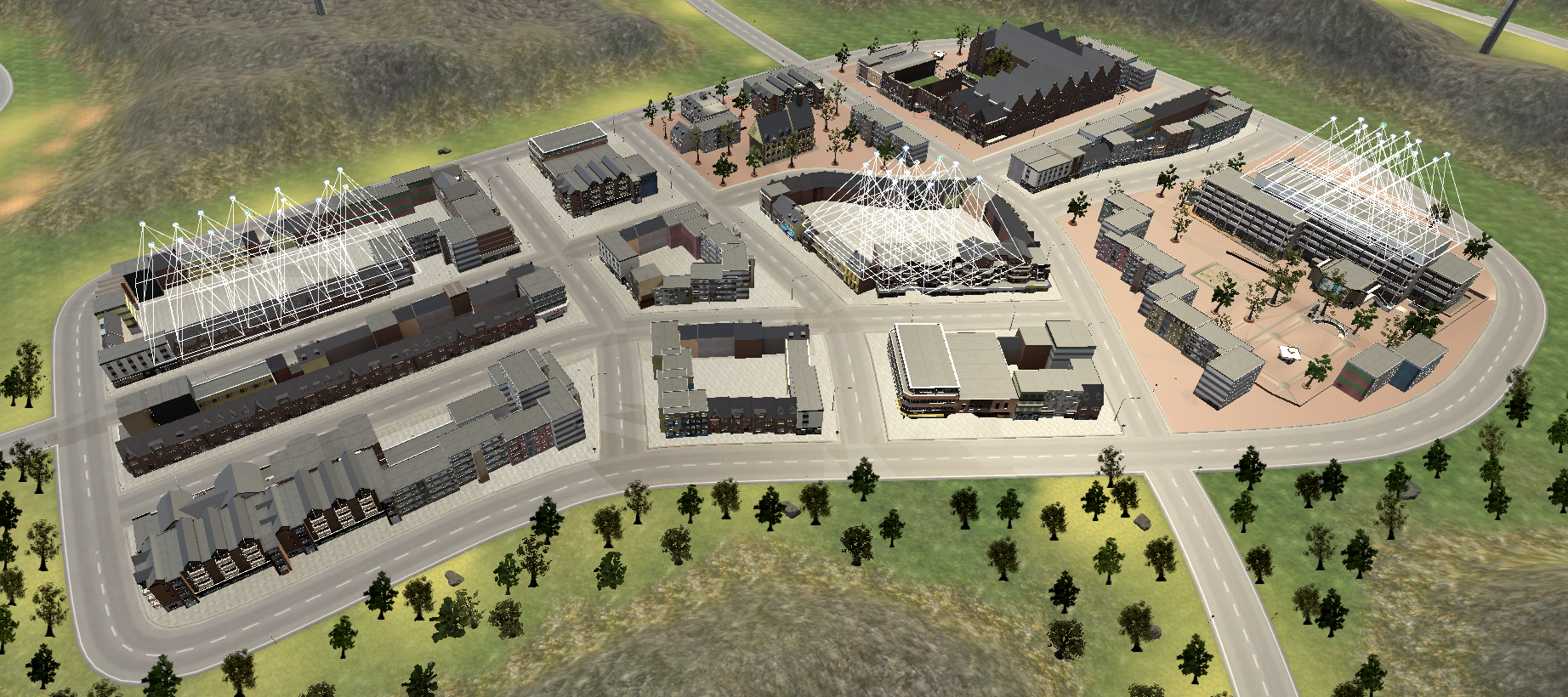
(a) The drones start from their initial deployment points.

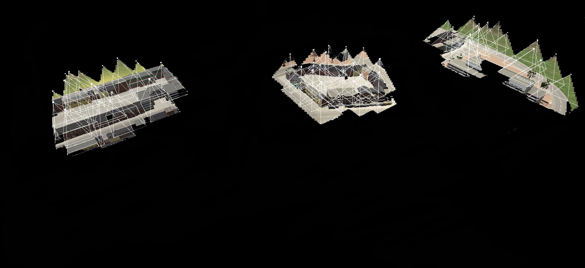
(b) Progress after 3 replanning steps.

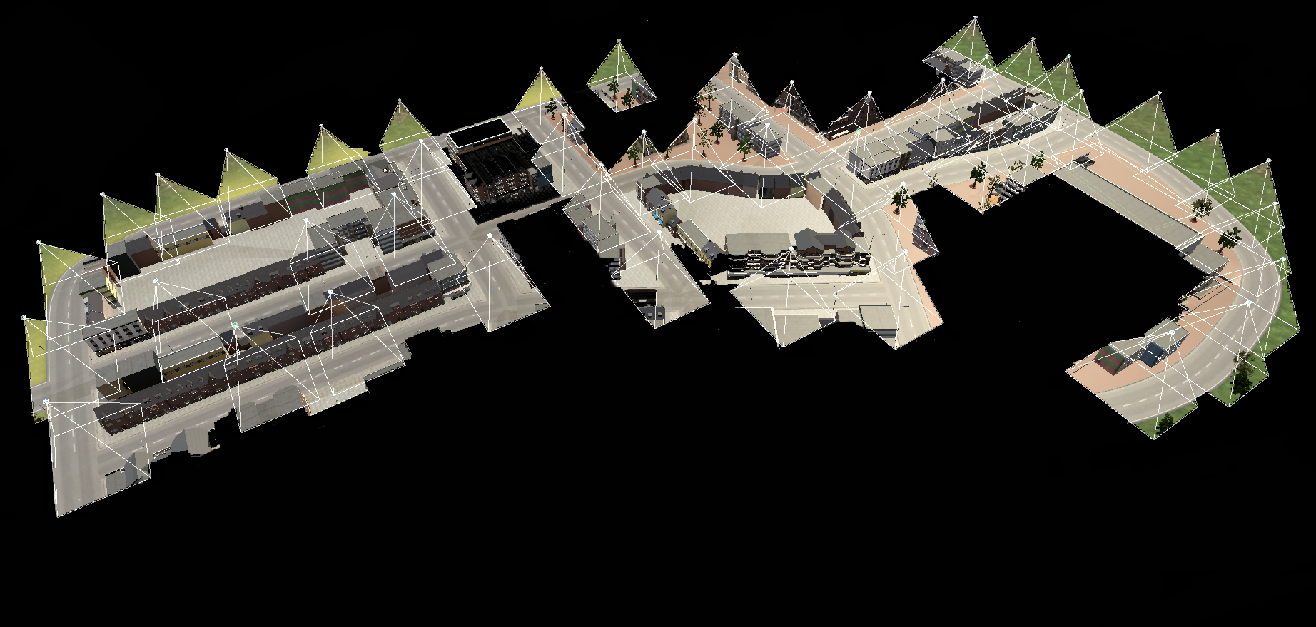
(c) Progress after 8 replanning steps.

Figure 1: Scenario of Collaborative Road Detection and Coverage with 45 Aerial Robots. The drones are deployed in an unknown urban environment and tasked to collaboratively detect the roads and visually cover them. Particularly, the drones aim to collectively maximize the total covered road area in their top-view field of view (FOV). At each motion-planning step, each drone chooses a few others drones to coordinate with, subject to its onboard communication and computation bandwidth constraints. The full collaborative autonomy pipeline is depicted in Fig. 2. (a)–(c) depict the task progress across time: (a) The drones start from their initial deployment points; (b) Progress after 3 replanning steps; (c) The drones have achieved maximal road coverage.

will be choosing what information to receive and from who such that they can jointly plan actions in real-time, ensuring that their planned actions complement each other, instead of duplicating each other.

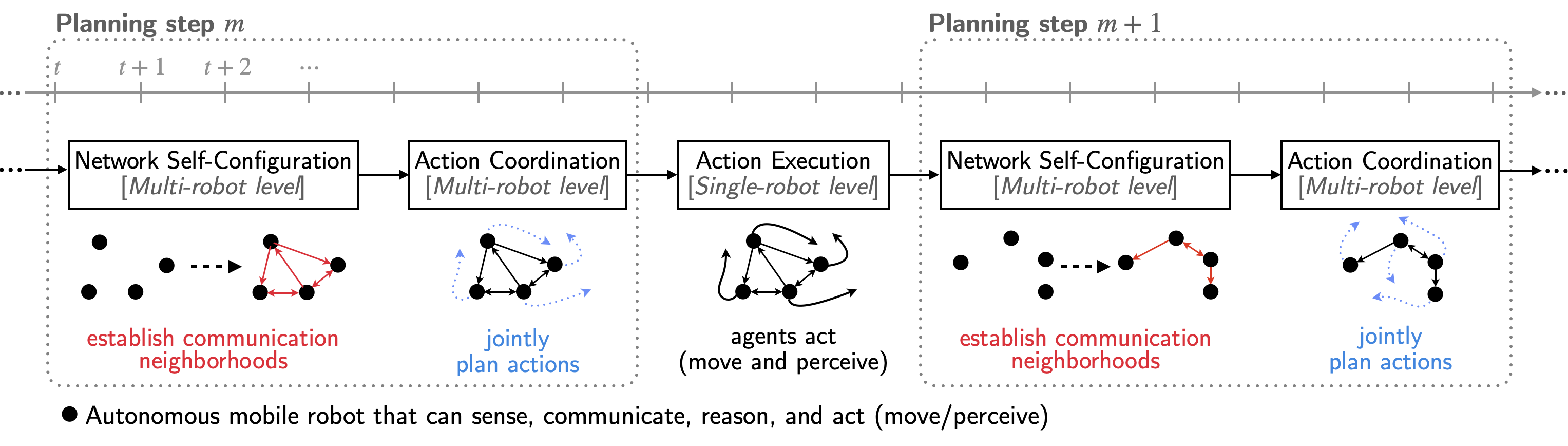
Figure 2: Pipeline of Collaborative Mobile Autonomy. The robots sequentially perform in a distributed manner: (a) Network Self-Configuration: Given the observed environment and state of the robots, the robots decide with which other robots to communicate with, subject to their onboard bandwidth constraints; and (b) Action Coordination: The robots jointly plan actions —how to move and sense the environment— upon coordinating over the established communication network. (c) Action Execution: The robots execute their selected actions and perceive the environment. In this paper, our focus is on Action Coordination. Particularly, we present a communication- and computation-efficient distributed algorithm that is up to two orders faster than the state-of-the-art near-optimal algorithms. We also provide an analysis of how the network topology at the robot level —neighborhood of each robot— affects the near-optimality of coordination. The analysis offers insights into how the robots may configure the network to balance (tune) the trade-off between decision speed and near-optimality.

However, these capabilities of efficiency and effectiveness are currently challenging to achieve. The current literature on distributed coordination via vehicle-to-vehicle (v2v) communication imposes a trade-off between decision speed and optimality. On the one hand, algorithms that minimize the action overlap among robots may not be real-time since they can require an explosion of information sharing and processing across the robot network: processing and transmitting information cannot happen instantaneously —in the context of multi-robot tasks such as mapping, surveillance, and target tracking, real-time may indicate a replanning frequency at the order of $1$Hz. On the other hand, heuristic approaches can be real-time but cannot guarantee minimal action overlap since they achieve rapid decision-making by heuristically limiting the coordination among a few, possibly randomly chosen, robots. We need algorithms that can balance the trade-off by enabling the robots to choose what information to receive and from who.

Contributions. We show that it is possible to balance the trade-off of decision speed and near-optimality. Particularly, we provide a rigorous coordination approach that enables robots to self-configure their communication neighborhood (the set of robots to coordinate with) to tune the trade-off, that is, prioritize decision speed over near-optimality, as needed. To this end, we make theoretical and algorithmic contributions as follows, introducing tools for distributed submodular optimization. Submodularity is a diminishing returns property typically arising in information gathering tasks such as the aforementioned ones; we introduce it rigorously in Section III.

On the theoretical side, we provide an analysis of how the network topology at the local level —neighborhood of each robot— affects the near-optimality of coordination at the global level (Section V). The characterization quantifies the intuition that the more centralized the coordination (with larger neighborhoods), the slower the decision speed but the smaller the action overlap. It thus offers insights into how the robots can configure their network to balance the trade-off of decision speed and near-optimality. Importantly, we identify the existence of an inflection point that corresponds to the degree of centralization that optimizes the trade-off: with larger neighborhoods, we prove that the decision time increases faster than the action overlap decreases. Therefore, beyond a degree of centralization, the cost of sacrificing real-time performance will be higher than the gain in the actions.

On the algorithmic side, we present a communication- and computation-efficient distributed coordination algorithm that can be both real-time and near-optimal (Section IV). The algorithm is up to two orders faster than the competitive state-of-the-art near-optimal algorithms (Section VI). In simulated scenarios of map exploration with up to 45 robots, where we also simulate v2v communication delays (Section VII), the algorithm achieves replanning frequencies at the order of $1$Hz with superior performance. The algorithm’s decision time scales linearly with the number of robots, and sublinearly when parallelization is possible. For example, parallelization is possible in spatially distributed settings where robots are far enough from one another and have little action overlap.

The algorithm’s approximation guarantee captures the intuition that when a robot chooses not to coordinate with some other robots but ends up choosing an action that overlaps with these non-neighbors, then the achievable global optimality degrades. Specifically, we prove that the suboptimality degradation is proportional to the overlap. To enable our analysis, we quantify the suboptimality cost as a function of the action overlap between a robot and its (non-)neighbors. We introduce to this end a mutual-information-like quantity over sets that we term Centralization of Information.

The algorithm is built on a resource-aware distributed coordination framework introduced in Section III. The framework is resource-aware in that it requires each robot to coordinate actions with its neighbors only, receiving and processing information only about them instead of more robots in the network. As such, the framework is communication- and computation-efficient, curbing the explosion of information passing and processing in the network, thus, keeping low the delays due to limited computation and v2v communication speeds.

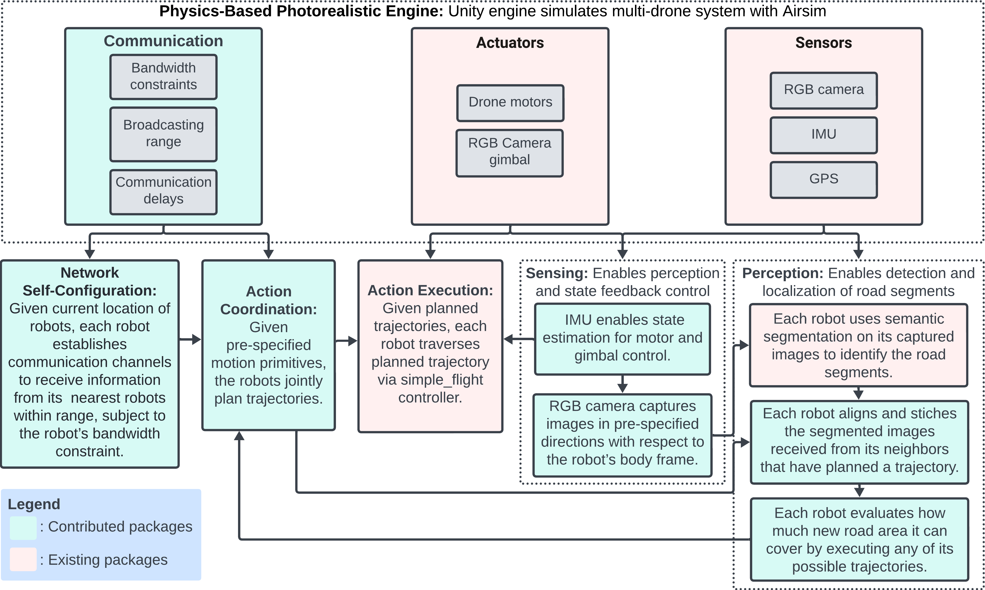
Figure 3: Simulator pipeline. We provide a high-fidelity simulator that extends AirSim [4] to the multi-robot setting by integrating the autonomy pipeline of Fig. 2 and simulating v2v communication delays among other communication constraints. The illustrated pipeline is customized for the action coordination algorithm provided herein. The pipeline can be modified to other algorithms as desired. The code will be open sourced via a link in this paper.

Simulator. To demonstrate the efficiency and effectiveness of our coordination algorithm, we integrate it in a simulated state-of-the-art pipeline for active information-gathering with multiple robots (Fig. 3). To this end, we provide a high-fidelity simulator that extends AirSim [4] to the multi-robot setting, simulating v2v communication delays. Although the “vanilla” AirSim provides a simulation framework with a physics engine, flight controller, inertial sensors, and vision-based sensors, it provides no native support for multi-robot coordination that involves task orchestration and simulates no v2v communication delays. To enable such support, we develop appropriate frameworks and APIs. We will open-source the code upon the acceptance of the paper.

Evaluation. We tested the algorithm in the simulator over scenarios of collaborative mapping for road coverage with $15$ and $45$ robots (Fig. 1), respectively. Our algorithm yields practical advantages. In the case of $15$ robots, the algorithm achieves both superior road area coverage and real-time planning, at the order of $1$ Hz, being one to two times faster than the competitive state-of-the-art algorithms. In the case of $45$ robots, the robots are deployed into three spatially separated teams each of $15$ robots so parallelized decision-making is made possible. The algorithm demonstrates its ability to automatically scale with the decision time growing sublinearly. In more detail, it maintains superior road coverage and achieves similar planning time as in the case of $15$ robots, being at most 2 times slower. In contrast, the competitive state of the art is now 15 times slower.

Organization of the Remaining Paper. In the following paragraphs, we compare with our preliminary work [5] and [6]. Then, in Section II, we present background on distributed coordination and related work. In Section III, we define the problem of Resource-Aware Distributed Coordination. Then, we present our algorithm in Section IV. The theoretical analysis of the algorithm’s approximation guarantees and decision time are presented in Sections V and VI, respectively. Section VII presents the simulator and the evaluation. Proofs not presented in the main text are presented in the appendix.

Comparison with Preliminary Work [5] and [6]. This paper extends our preliminary work [5] to include new theory, the AirSim simulator implementation, the evaluations on the simulator, and proofs of all claims. Particularly, this paper provides novel performance guarantees, including an a posteriori bound with network-design implications, and an extension of the a priori bound in [5] to functions that are not submodular. Also, this paper bounds the decision time of the algorithm, characterizing for the first time its communication and computation complexity as a function of the size of the network and the times to perform computations and v2v communications. This paper introduces the AirSim-based simulator and the evaluations on the simulator. Instead, [5] employed MATLAB simulations only without simulating v2v communication delays. All proofs were omitted in [5], and here are presented for all original and new results.

We also compare this paper with the pre-print that is under review for conference publication [6]. First of all, [6] introduces a different problem formulation from the one in eq. 1, requiring the communication-network topology to be co-optimized with the robots’ actions. The solution provided therein requires sensors/robots at fixed locations, instead of mobile sensors/robots, which are the focus herein. Finally, the results in [6] hold in probability and are based on regret optimization that requires quadratic time to converge, whereas the results herein are deterministic and are based on discrete optimization that requires linear time to converge.

II Background and Related Work

We first present background on distributed coordination, and explain that distributed coordination can be hard since it often takes the form of submodular set-function maximization, which is NP-hard. Then, we discuss the state of the art.

II-A Background on Distributed Coordination

Distributed coordination via v2v communication is challenging in multi-robot tasks such as mapping, surveillance, and target tracking, modeled as submodular set-function optimization problems [7, 2, 8, 9, 1, 3, 10, 11, 12, 13, 14], which are NP-hard [15, 16]. Submodularity is a diminishing returns property, capturing the intuition that when the same information is collected by two or more robots, its value to the task cannot be double-counted. Thereby, submodular multi-robot tasks are difficult to efficiently solve even in centralized settings. Rigorously, submodular multi-robot tasks take the optimization form:

$$\max_{a_{i}\,\in\,\mathcal{V}_{i},\,\forall\,i\,\in\,{\cal N}}\ f(\,\{a_{i}\}_{i\,\in\,{\cal N}}\,),$$ (1)

where ${\cal N}$ is the set of robots, $a_{i}$ is robot $i$’s action, $\{a_{i}\}_{i\,\in\,{\cal N}}$ is the ordered set of all robots’ actions, ${\cal V}_{i}$ is robot $i$’s set of available actions, and $f\colon 2^{\prod_{i\in{\cal N}}{\cal V}_{i}}\mapsto\mathbb{R}$ is the objective function that captures the (submodular) task utility.

For example, in road coverage with multiple drones (Fig. 1), ${\cal N}$ is the set of drones, ${\cal V}_{i}$ is the set of available trajectories the drone $i$ can choose from, and $f$ is the total road area covered by the drones’ collective field of view by the time their actions have been executed. This $f$ can be shown to be submodular. Intuitively, if two drones observe the same road area upon executing their actions, then either of the drones is redundant in the presence of the other. Therefore, to maximize the total covered road area, the drones need to minimize their action overlap via coordination.

Within the collaborative autonomy pipeline in Fig. 2, the optimization problem in eq. 1 models the action coordination stage, that is, the stage where robots jointly plan actions over a look-ahead horizon of optimization. Then, upon making the joint plans, each robot individually executes its action in a receding-horizon fashion till its action is updated via the subsequent coordination stage.

II-B Related Work

We discuss the related work across four dimensions: (i) near-optimal but not necessarily real-time coordination algorithms; (ii) rapid but not necessarily near-optimal coordination algorithms; (iii) works on the trade-off between decision speed and optimality; and (iv) communication simulators.

Near-optimal coordination algorithms

Although current approximation paradigms for the submodular maximization problem in eq. 1 [17, 16, 18] enable the robots to near-optimally minimize their action overlap [7, 2, 8, 9, 1, 3, 10, 11, 12, 13, 14], they may not be real-time. The reason is that their communication and computation complexities are superlinear in the number of robots, particularly, quadratic or cubic (we will elaborate on this later). Instead, we provide an algorithm with linear communication and computation complexity.

Quadratic or higher communication and/or computation complexity can become prohibitive in large-scale networks due to real-world communication and computation delays. To illustrate the point, we give a toy example upon noting that communication delays are introduced by the limited v2v communication speeds. For example, state-of-the-art v2v communication speeds range from less than $1$Mbit/sec up to $125$MBytes/sec [19]. Computational delays are caused by the time required to perform function evaluation. This time depends on the processing required by the task at hand, e.g., image segmentation for the said task of road coverage (Fig 1). Assume now that the total delay per communication and computation is on average $1$msec. Then, for cubic decision-time complexity and $100$ robots ($|{\cal N}|=100$), the total time delay is at the order $100^{3}\cdot 1\text{msec}\simeq 17\text{min}$. This is three orders higher than the desired $\simeq 1Hz$ planning frequency.

The quadratic or higher complexity of [17, 16, 18] over v2v networks is due to their coordination protocols: they instruct the robots to retain and relay information about all or most other robots in the network. Particularly, [17, 16] require iterative decision-making via consensus where at each iteration each robot needs to retain and transmit estimates of all robots’ actions [17, 16]. [18] requires sequential decision-making where all currently finalized actions need to be relayed to all robots in the network that have not finalized actions yet.

In more detail, the multi-robot coordination algorithm in [20], inspired by [17, 16, 18], achieves the best possible approximation bound for the maximization problem in eq. 1, namely, $1-1/e$. However, it may require tenths of minutes to terminate in simulated tasks of $10$ robots even with no simulated communication delays [5]. The reason is that it requires a near-cubic number of iterations in the number of robots to converge (Table I). Similarly, for the Sequential Greedy (SG) algorithm [18], also known as Coordinate Descent, which is the gold standard in robotics and control for the maximization problem in eq. 1 [7, 2, 8, 3, 9, 1, 10, 11, 12, 13, 14], although it sacrifices some approximation performance to enable faster decision speed —achieving the bound $1/2$ instead of the bound $1-1/e$— still requires inter-robot messages that carry information about all the robots and, in the worst case, a quadratic number of communication rounds over directed networks [21, Proposition 2], resulting in the communication complexity being cubic in the number of robots [6, Appendix II].

Real-time coordination algorithms

To achieve real-time planning, state-of-the-art coordination algorithms employ approaches that do not account for the submodular structure of the multi-robot task at hand. Thus, although fast, these approaches provide no guarantee that the agents’ joint actions will have minimal overlap. For example, in the context of collaborative exploration, the robots coordinate actions to move to the closest frontiers using shared map information in [22]. [23, 24, 25, 26] use an auction-based mechanism for task allocation among robots. In particular, the auction is also leveraged for high-probability communication maintenance in [25]. In [27], robots are assigned to different frontiers based on potential functions for distributed mapping and exploration. The robots set periodic meeting destinations in [28] to meet and coordinate actions during distributed exploration. [29] introduces a pair-wise coordination protocol where all pairs of neighboring robots sequentially coordinate trajectories to optimize their exploration task allocation. A similar pair-wise coordination protocol is proposed in [30] where each robot coordinates trajectories with the neighbor that it has longest not communicated with to minimize their overall trajectories.

Additionally, the said approaches are application-specific, e.g., exploration for the case of [28, 30], whereas, our theoretical and algorithmic results are general-purpose.

Characterization of the trade-off between decision speed and optimality

To enable rapid distributed coordination at scale, we need to curtail the information explosion in multi-robot networks, thereby, need to limit what and how much information can travel across the network. However, the impact of imposing such information limitations is suboptimal actions.

Current works have captured the suboptimality cost due to such information access for the case of the Sequential Greedy algorithm [31, 32, 12]. However, the provided characterizations are task-agnostic, considering the worst-case over all possible submodular functions and action sets.

In contrast, in this paper, the suboptimality cost is captured as a direct function of the action overlap over the task objective $f$ at hand and the robots’ chosen actions. Even if all robots plan in isolation, the guaranteed performance can still match the near-optimal $1/2$, if the robots’ chosen actions do not overlap, instead of being inversely proportional to the number of agents that would be the case for [31, 32, 12].

Also, to our knowledge, our characterizations are the first to quantify the suboptimality cost as a function of each agent’s local communication network of agents. The practical implication is that the characterizations can be used to enable the robots to select their communication neighborhoods to tune the trade-off of decision speed and near-optimality, subject to their communication bandwidth constraints.

Communication simulators for multi-robot applications

In information-heavy collaborative tasks such as mapping, surveillance, and target tracking, capturing how v2v communication delays can compromise the efficiency of multi-robot decision-making becomes important. Therefore, in this paper, given our focus on communication-efficient distributed decision-making, we indeed integrate in the AirSim pipeline v2v communication delays (Fig. 3).

For completeness, we next discuss papers that provide higher-fidelity simulations of wireless communication, including packet losses and occlusions. Particularly, [33] simulates the communication delay and demonstrates its influence in consensus-based applications. [34, 35, 36] simulate the communication channels and protocols and demonstrate how the communication delay between two robots will be impacted by the distance and line-of-sight conditions between them. [37] simulates realistic propagation models and scheduling functions for mobile radio-frequency (RF) communications and shows they can degrade task performance.

In our future work, we will integrate in the AirSim simulator such simulation capabilities to enable the testing of communication-aware and -efficient algorithms for distributed submodular coordination.

III Resource-Aware Distributed Coordination

We define the problem of Resource-Aware Distributed Coordination (1) with regard to the action coordination module in Fig. 2. To this end, we use the notation:

• ${\cal E}$ is the set of communication channels among the robots;

• ${\cal V}_{\cal N}\triangleq\prod_{i\,\in\,{\cal N}}\,{\cal V}_{i}$ is the cross-product of sets $\{{\cal V}_{i}\}_{i\,\in\,{\cal N}}$;

• $f(a\,|\,{\cal A})\triangleq f({\cal A}\cup\{a\})-f({\cal A})$ is the marginal gain due to adding $a$ to ${\cal A}$, given a set function $f:2^{{\cal V}}\mapsto\mathbb{R}$.

We also lay down the following framework for the robot-to-robot communication network and the objective function that captures the multi-robot task at hand.

Communication Neighborhood. At the beginning of each planning step (Fig. 2), given the observed environment and state of the robots, the robots decide with which others to establish communication, subject to their onboard bandwidth constraints. Specifically, we assume that each robot $i$ can receive information from up to $\alpha_{i}$ other robots due to onboard bandwidth constraints. Thus, it must be $|{\cal N}_{i}|\;\leq\alpha_{i}$. In Section V, we provide theoretical characterizations that inform how the robots may select their neighbors to optimize the coordination performance. In our simulations over a scenario of road coverage, the robots select their neighbors based on physical proximity, as justified by the results in Section V.

When a communication channel is established from robot $j$ to robot $i$, i.e., $(j\rightarrow i)\in{\cal E}$, then robot $i$ can receive, store, and process information from robot $j$. The set of all robots that robot $i$ receives information from is denoted by ${\cal N}_{i}$. We refer to ${\cal N}_{i}$ as robot $i$’s neighborhood.

Communication Network. The resulting communication network can be directed and even disconnected. When the network is fully connected (all robots receive information from all others), we call it fully centralized. In contrast, when the network is fully disconnected (all robots receive no information from other robots), we call it fully decentralized.

We assume communication to be synchronous.

Communication Data Rate. All communication channels $(j\rightarrow i)\in{\cal E}$ have finite data rate, i.e., communication speed. In the simulations, we assume the data rate is $10$MBytes/sec, in accordance with typical v2v communication speeds [38]. Due to the finite data rate, the decision time of action coordination depends on both (i) the number of communication rounds and (ii) the size of transmitted messages it requires for the robots to find a joint plan. Without loss of generality, we assume all communication channels have the same data rate in this paper.

Objective Function. The robots coordinate their actions to maximize an objective function. In active information gathering tasks, such as area coverage, target tracking, and persistent monitoring, typical objective functions are the covering functions [39, 20, 40]. These functions capture how much area/information is observed given the actions of all robots. They satisfy the properties below (Definitions 1 and 2).

Definition 1 (Normalized and Non-Decreasing Submodular Set Function [18]).

A set function $f:2^{\cal V}\mapsto\mathbb{R}$ is normalized and non-decreasing submodular if and only if

• $f(\emptyset)=0$;

• $f({\cal A})\leq f({\cal B})$, for any ${\cal A}\subseteq{\cal B}\subseteq{\cal V}$;

• $f(s\,|\,{\cal A})\geq f(s\,|\,{\mathcal{B}})$, for any ${\cal A}\subseteq{\mathcal{B}}\subseteq{\cal V}$ and $s\in{\cal V}$.

Normalization $(f(\emptyset)=0)$ holds without loss of generality. In contrast, monotonicity and submodularity are intrinsic to the function. Intuitively, if $f({\cal A})$ captures the area covered by a set ${\cal A}$ of activated cameras, then the more sensors are activated $({\cal A}\subseteq{\cal B})$, the more area is covered $(f({\cal A})\leq f({\cal B}))$; this is the non-decreasing property. Also, the marginal gain of covered area caused by activating a camera $s$ drops $(f(s\,|\,{\cal A})\geq f(s\,|\,{\mathcal{B}}))$ when more cameras are already activated $({\cal A}\subseteq{\cal B})$; this is the submodularity property.

Definition 2 (2nd-order Submodular Set Function [41, 42]).

$f:2^{\cal V}\mapsto\mathbb{R}$ is 2nd-order submodular if and only if

$$f(s)-f(s\,|\,{\cal A})\geq f(s\,|\,{\cal B})-f(s\,|\,{\cal A},\,{\cal B}),$$ (2)

for any disjoint ${\cal A}\subseteq{\cal V}$ and ${\cal B}\subseteq{\cal V}$ (${\cal A}\cap{\cal B}=\emptyset$) and $s\in{\cal V}$.

The 2nd-order submodularity is another intrinsic property to the function. Intuitively, if $f({\cal A})$ captures the area covered by a set ${\cal A}$ of cameras, then marginal gain of the marginal gains drops when more cameras are already activated.

Problem 1 (Resource-Aware Distributed Coordination).

Each robot $i\in{\cal N}$ independently selects an action $a_{i}$, using only information from and about its neighbors ${\cal N}_{i}$, such that the robot actions $\{a_{i}\}_{i\,\in\,{\cal N}}$ jointly solve the optimization problem

$$\max_{a_{i}\,\in\,\mathcal{V}_{i},\,\forall\,i\,\in\,{\cal N}}\;f(\,\{a_{i}\}_{i\,\in\,{\cal N}}\,).$$ (3)

1 is resource-aware in that it requires each robot to coordinate actions with its neighbors only, receiving information only about them instead of more robots in the network. The reason is to curtail the explosion of information passing across the network and, thus, to enable rapid decision-making. This is in contrast to standard distributed methods that allow information about the whole network to travel to all other robots via information passing, i.e., multi-hop communication [21, 39, 43]. Multi-hop communication does not reduce the amount of information flowing in the network compared to centralized methods, introducing impractical communication delays, as we will demonstrate in the simulations.

In the resource-aware framework of 1, the network configuration affects the achievable maximal value of $f$ in 3 since the network configuration decides what information becomes available to each of the robots. For example, in a fully decentralized network where all robots select actions in isolation, the achievable value of $f$ will be lower than the achievable value in a fully centralized network where all robots coordinate with each other and jointly select actions. Similarly, consider a scenario where the robots are identical mobile cameras that start from the same location and have the same options to move around, and where $f$ is the union of the area covered by the robots’ FOVs. Then, in the fully decentralized setting, all robots may end up looking at the same area, due to the lack of any coordination. Thus, $f$ will be equal to the area covered by one robot since all robots’ views overlap. In contrast, in the fully centralized setting, the robots can coordinate to avoid overlapping their FOVs, thus maximizing the total covered area $f$.

In this paper, we provide an analysis of how the network topology at the local level —each robot’s neighborhood ${\cal N}_{i}$— affects the near-optimality of coordination at the global level. The analysis applies over the spectrum from fully decentralized to fully centralized networks, offering insights into how the robots may tune the sparsity of the network to balance the trade-off between decision speed and near-optimality.

Along with the theoretical characterizations above, we also provide a communication-efficient distributed algorithm that requires only a few coordination rounds and exchanging short messages among the robots, per the limited information-sharing setting of 1, and that is up to two to three orders faster than the state-of-the-art near-optimal algorithms. The algorithm is presented next.

IV Resource-Aware distributed Greedy (RAG) Algorithm

10:  ​robot $i$’s actions $\mathcal{V}_{i}$; neighborhood ${\cal N}_{i}$;

non-decreasing set function $f:2^{\mathcal{V}_{\cal N}}\mapsto\mathbb{R}$;

20:  robot $i$’s action $a^{{\sf RAG}}_{i}$.

31:  ${\cal I}_{i}\leftarrow\emptyset$;   ${\cal A}_{i}\leftarrow\emptyset$;   $a^{{\sf RAG}}_{i}\leftarrow\emptyset$; // ​${\cal I}_{i}$ is the robots

in ${\cal N}_{i}$ that have selected their actions; ${\cal A}_{i}$ stores ${\cal I}_{i}$’s selected actions; $a_{i}^{\sf RAG}$ is robot $i$’s selected action

2:  while $a^{{\sf RAG}}_{i}=\emptyset$ do

3:     $a_{i}\leftarrow\arg\max_{a\,\in\,\mathcal{V}_{i}}\,f({\cal A}_{i}\cup\{a\})-f({\cal A}_{i})$;

4:     $g_{i}\leftarrow f({\cal A}_{i}\cup\{a_{i}\})-f({\cal A}_{i})$;

5:     receive $\{g_{j}\}_{j\,\in\,{\mathcal{N}_{i}\setminus{\cal I}_{i}}}$;

6:     if $i=\arg\max_{j\,\in\,\mathcal{N}_{i}\cup\{i\}\setminus{\cal I}_{i}}\,g_{j}$ then

7:        $a^{{\sf RAG}}_{i}\leftarrow a_{i}$; // $i$ has the best action candidate across $\mathcal{N}_{i}\cup\{i\}\setminus{\cal I}_{i}$ and it selects this action candidate

8:        broadcast $a^{{\sf RAG}}_{i}$ to out-neighbors; // out-neighbors can be different from ${\cal N}_{i}$

9:     else

410:        denote as ${\cal S}^{{\sf new}}_{i}\subseteq{\cal N}_{i}\setminus{\cal I}_{i}$ the set of neighbor(s)

that just selected action(s) in this iteration; // ${\cal S}^{{\sf new}}_{i}$ may be empty as we explain in Section IV-A

11:        receive $a^{{\sf RAG}}_{j}$ from each robot $j\in{\cal S}^{{\sf new}}_{i}$;

12:        ${\cal I}_{i}\leftarrow{\cal I}_{i}\cup{\cal S}^{{\sf new}}_{i}$;

13:        ${\cal A}_{i}\leftarrow{\cal A}_{i}\cup\{a^{{\sf RAG}}_{j}\}_{j\,\in\,{\cal S}_{i}^{{{\sf new}}}}$;

14:     end if

15:  end while

16:  return  $a^{{\sf RAG}}_{i}$.

Algorithm 1 Resource-Aware distributed Greedy (RAG).

	RAG: Terminates in $2\,\tau_{f}\,|{\cal V}_{i}|\,+\,\tau_{c}\,+\,\tau_{\#}$				SG: $5\,\tau_{f}\,|{\cal V}_{i}|\,+\,10\,\tau_{c}$
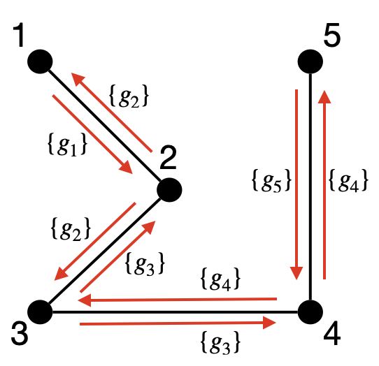
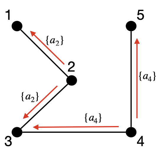
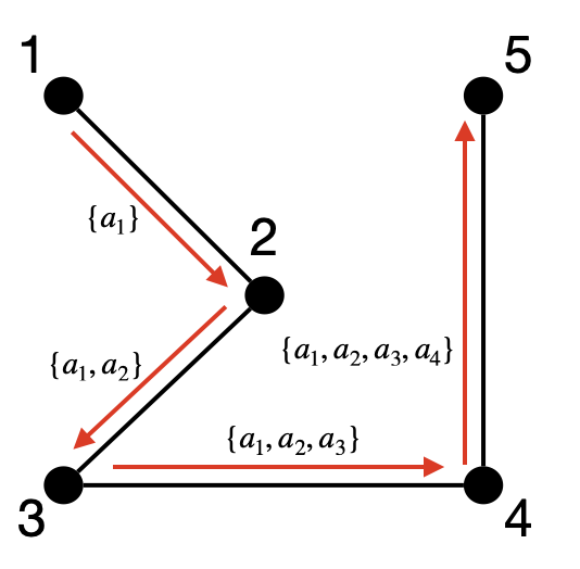
Line Graph	(a) The 1st iteration of RAG starts. Each agent $i$ simultaneously finds its action candidate $a_{i}$ with the largest marginal gain $g_{i}$ from all available actions ${\cal V}_{i}$. The operation takes $\tau_{f}\,|{\cal V}_{i}|$.	(b) Each agent $i$ simultaneously receives $g_{j}$ from each neighbor $j\in{\cal N}_{i}$. This takes $\tau_{\#}$. Then, it compares $g_{i}$ with them. We assume $g_{2}=\max{(g_{1},g_{2},g_{3})}$ and $g_{4}=\max{(g_{3},g_{4},g_{5})}$.	(c) Thus, agents 2 and 4 get to select actions. Agents 1, 3, 5 simultaneously receive the actions selected by their neighbors. This takes $\tau_{c}$. The 1st iteration ends. Only 1, 3, 5 continue.	(d) The 2nd iteration starts. Given the received actions, agents 1, 3, 5 simultaneously select actions. This requires $\tau_{f}\,|{\cal V}_{i}|$. Then all agents have selected actions, and RAG terminates.	(e) Sequentially, from $i=1$ to $5$, agent $i$ receives $\{a_{1},$ $\dots,a_{i-1}\}$, in $\tau_{c}\,(i-1)$ time, then selects $a_{i}$, which takes $\tau_{f}\,|{\cal V}_{i}|$ time, and then transmits $\{a_{1},\dots,a_{i}\}$ to agent $i+1$.
	RAG: Terminates in $2\,\tau_{f}\,|{\cal V}_{i}|\,+\,\tau_{c}\,+\,\tau_{\#}$				SG: $5\,\tau_{f}\,|{\cal V}_{i}|\,+\,17\,\tau_{c}$
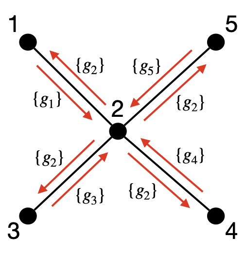
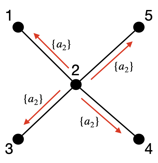
Star Graph	(f) The 1st iteration of RAG starts. Each agent $i$ simultaneously finds its action candidate $a_{i}$ with the largest marginal gain $g_{i}$ from all available actions ${\cal V}_{i}$. The operation takes $\tau_{f}\,|{\cal V}_{i}|$.	(g) Each agent $i$ simultaneously receives $g_{j}$ from each neighbor $j\in{\cal N}_{i}$. This takes $\tau_{\#}$. Then, it compares $g_{i}$ with them. We assume $g_{2}=\max{(g_{1},g_{2},g_{3},g_{4},g_{5})}$.	(h) Thus, agent 2 gets to select an action. Agents 1, 3, 4, 5 simultaneously receive the action selected by their neighbor. This takes $\tau_{c}$. The 1st iteration ends. Only 1, 3, 4, 5 continue.	(i) The 2nd iteration starts. Given the received action, agents 1, 3, 4, 5 simultaneously select actions. This requires $\tau_{f}\,|{\cal V}_{i}|$. Then all agents have selected actions, and RAG terminates.	(j) From $i=1$ to $5$, agent $i$ receives $\{a_{1},\dots,a_{i-1}\}$, possibly via $r_{i}$ relay nodes (takes $\tau_{c}\,(r_{i}+1)\,(i-1)$), then selects $a_{i}$ (takes $\tau_{f}\,|{\cal V}_{i}|$), and then transmits $\{a_{1},\dots,a_{i}\}$ to agent $i+1$.

Figure 4: RAG vs. Sequential Greedy (SG) [18]. The two algorithms are compared in their execution steps and in the time they need to terminate when they are run by five agents in two scenarios with the communication networks being: (i) an undirected line graph and (ii) an undirected star graph, respectively. In the figure, nodes $1$ to $5$ are the agents $1$ to $5$; black lines are undirected communication links; $\{a_{i},g_{i}\}$ denotes agent $i$’s newly updated action candidate $a_{i}$ with marginal gain $g_{i}$; $\{a_{i}\}$ and $\{g_{i}\}$ alongside red arrows are the actions and marginal gain values being transmitted between two agents; the transparent nodes are the agents that have selected their actions and thus already ended running RAG; and the transparent edges are the communication channels that have become “disappeared” since at least one end of them has finished RAG. The implementation of RAG ((a)–(d) and (f)–(i)) results in way shorter decision time than SG ((e) and (j)) in both scenarios with the line and star graphs, respectively.

We present the Resource-Aware distributed Greedy (RAG) algorithm. Examples of how the algorithm works are given in Fig. 4. Therein, we also compare RAG to the Sequential Greedy algorithm (SG) [18]. SG is the “gold standard” in submodular maximization. SG is presented in (Section IV-B).

IV-A The Resource-Aware distributed Greedy (RAG) Algorithm

The pseudo-code of RAG, as it is used onboard an robot $i$, is presented in Algorithm 1. The purpose of each iteration of RAG, namely, of each “while loop” (lines 2–15), is to enable robot $i$ to decide whether to select an action over its neighbors at this iteration or to pass because a neighbor has an action with a higher marginal gain. If passing, then the robot must wait for a future iteration to select an action. In more detail, at each “while loop”:

• robot $i$ finds an action $a_{i}$ with the highest marginal gain $g_{i}$ given the actions selected by neighbors ${\cal I}_{i}\subseteq{\cal N}_{i}$ so far (lines 3–4).

• robot $i$ receives the respective highest marginal gain $g_{j}$ of all neighbors $j$ that have not selected an action yet, namely, of all $j\in{\cal N}_{i}\setminus{\cal I}_{i}$ (line 5).

• robot $i$ compares $g_{i}$ with all $g_{j}$’s (line 6).

• If $g_{i}>g_{j},\forall j\in\mathcal{N}_{i}\setminus{\cal I}_{i}$, then robot $i$ selects $a_{i}$, i.e., $a_{i}^{\sf RAG}\leftarrow a_{i}$, broadcast $a_{i}^{\sf RAG}$, and RAG terminates onboard robot $i$ (lines 6–8 and 2, respectively).

• Otherwise, robot $i$ passes (line 9), and receives the actions selected at this iteration by its neighbors with the highest marginal gain among their respective neighbors, if any (line 11) —the set of these neighbors is denoted as ${\cal S}_{i}^{{\sf new}}$ (line 10). Particularly, ${\cal S}^{{\sf new}}_{i}$ may be empty if no neighbor can select an action per their onboard iteration of RAG.

Remark 1 (Directed, Possibly Disconnected Communication Topology).

RAG is valid for directed and even disconnected communication topologies. For example, RAG can be applied to a robot $i$ that is completely disconnected from the network.

IV-B Comparison to the Sequential Greedy algorithm (SG)

RAG is compared with SG [18] in Fig. 4. We rigorously present SG next, and provide a qualitative comparison with RAG. Rigorous comparisons in terms of runtime and approximation performance are postponed to Sections V and VI.

SG instructs the robots to sequentially select actions such that the $i$-th robot in the sequence selects

$$a_{i}^{\sf SG}\,\in\,\max_{a\,\in\,{\cal V}_{i}}\;\;f(\,a\;|\;\{a_{1}^{\sf SG},\ldots,a_{i-1}^{\sf SG}\}\,);$$ (4)

i.e., $a_{i}^{\sf SG}$ maximizes the marginal gain over the actions that have been selected by the $i-1$ previous robots in the sequence. In contrast, RAG enables the robots to select actions in parallel, and even if not all their neighbors have selected an action.

The above action-selection features of RAG —parallelization and action selection before all neighbors have chosen an action— can speed up the algorithm’s termination, as we rigorously present in Section VI. Also, they enable RAG to work on arbitrary communication topologies, a fact that can further contribute to faster runtimes. For example, SG requires a line path connecting all robots in the action-selection sequence. If such a path does not exist (see star graph example in Fig. 4), the $i$-th robot in the action-selection sequence cannot necessarily communicate directly with the $(i+1)$-th robot. Then, SG requires extra communication rounds for message relaying, further delaying its termination. Specifically, given the limited communication speed of robot-to-robot communication channels [38], the termination of SG is delayed due to both the increased number of communication rounds, and the communication delay incurred from relaying the actions of multiple robots —the robots in the sequence that have chosen an action so far— across the network.

V Approximation Guarantees:
Centralization vs. Decentralization Perspective

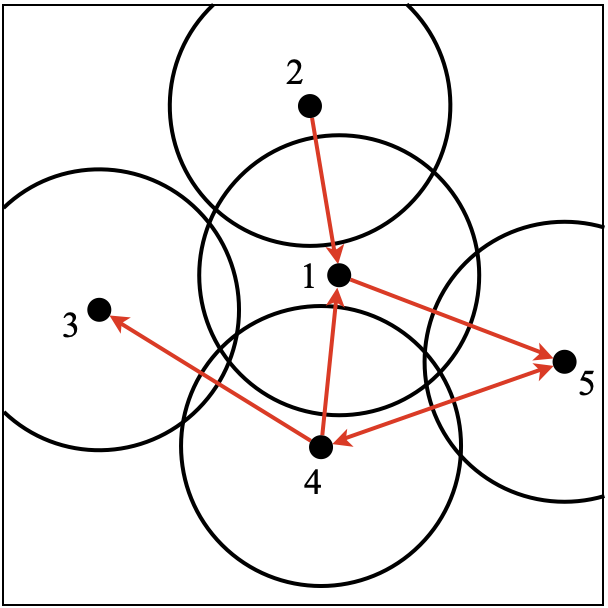
(a) Setup. The robots are tasked to maximize the area covered among the available square area by picking locations to stay at. Each robot (dot) has a field of view (circle), and established communication channels with its neighbors (red arrows). For example, for robot $1$, its neighbors are the robots in ${\cal N}_{1}=\{2,4\}$, thus its non-neighbors are those in ${\cal N}_{1}^{c}=\{3,5\}$.

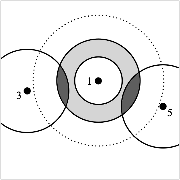
(b) Robot $1$’s non-neighbors ${\cal N}_{1}^{c}$, ${\sf coin}_{f,1}({\cal N}_{1})$, and worst-case ${\sf coin}_{f,1}$. The non-neighbors ${\cal N}_{1}^{c}=\{3,5\}$ are the robots that robot $1$ does not communicate range, e.g., because of limited bandwidth or because they are outside its communication range (dashed circle). ${\sf coin}_{f,1}({\cal N}_{1})$ is depicted by the dark gray area, and its upper bound the light gray ring area (Example 1).

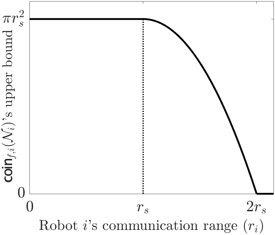
(c) Computable upper bound of ${\sf coin}_{f,i}$ as a function of robot $i$’s communication range. $r_{s}$ is the robots’ sensing radius (Example 1).

Figure 5: Multi-Robot Network for Area Coverage. (a) A scenario with $5$ robots, their communication network, and a limited square area that the robots are tasked to cover; (b) Illustration of robot $1$’s non-neighbors ${\cal N}_{1}^{c}$, ${\sf coin}_{f,1}({\cal N}_{1})$, and worst-case ${\sf coin}_{f,1}$ ${\sf coin}_{f,1}({\cal N}_{1})$; (c) Computable upper bound of ${\sf coin}_{f,i}$ as a function of robot $i$’s communication range per the analysis in Example 1.

We present the a priori and posteriori suboptimality bounds of RAG (Theorems 1 and 2). They both capture the suboptimality cost due to decentralization, that is, due to each agent coordinating only with a few agents —its neighbors— and receiving information only about them, in favor of decision speed.

The two bounds are useful as follows: The a priori bound enables each agent to design its neighborhood to minimize its local suboptimality cost subject to its communication-bandwidth constraints. The a posteriori bound results in two practical observations: first, decentralized coordination can marginally be as near-optimal as centralized coordination (Remark 7); second, larger neighborhoods do not necessarily result in better coordination performance when we account for both the decision time and the suboptimality of the algorithm (Remark 8). We validate and leverage the above in the experimental results of Section VII.

In the following paragraphs, we first introduce the novel notion of Centralization of Information to quantify the a priori suboptimality bound (Section V-A). Then, we present first the a priori bound of RAG that involves the proposed novel notion (Section V-B) and second the a posteriori bound (Section V-C). Finally, we compare the a priori bound with the a priori bounds in the state of the art (Section V-D).

V-A Centralization of Information

We introduce the notion of centralization of information (${\sf coin}$). In Section V-B, we use the notion to quantify the suboptimality cost due to decentralization. Particularly, ${\sf coin}$ measures how the agents’ actions overlap due to the agents not coordinating with their non-neighbors. We also relate ${\sf coin}$ to the classical notion of total curvature [44] and to pair-wise consistency [39] (Remarks 2 and 3), and show that ${\sf coin}$ is a less conservative measure of action overlap.

We use the following notation and definition:

• $\mathcal{N}_{i}^{c}\triangleq\mathcal{N}\setminus\{\mathcal{N}_{i}\cup\{i\}\}$ is the set of robot $i$’s non-neighbors, i.e., the robots beyond $i$’s neighborhood (see Fig. 5(b)).

• The total curvature [44] of a function $f\colon 2^{{\cal V}_{\cal N}}\mapsto\mathbb{R}$ that is non-decreasing and submodular, and that, without loss of generality, $f(a)\neq 0$, for any agent’s action $a$, i.e., for any $a\in\bigcup_{i\,\in\,{\cal N}}{\cal V}_{i}$, is defined as:

  $$\kappa_{f}\triangleq 1-\min_{{\cal A}\,\in\,{\cal V}_{\cal N}}\;\min_{a\,\in\,{\cal A}}\;\frac{f({\cal A})-f({\cal A}\setminus\{a\})}{f(a)}.$$ (5)

  $\kappa_{f}$ measures how the action $a$ of an agent can overlap with the actions of all other agents in the worst case. Particularly, $\kappa_{f}\in[0,1]$, and if $\kappa_{f}=0$, then $f({\cal A})-f({\cal A}\setminus\{a\})=f(a)$, for all $a\in{\cal A}$, i.e., the action $a$ of an agent does not overlap with the actions of any other agents. In contrast, if $\kappa_{f}=1$, then there exists $a\in{\cal A}$ such that $f({\cal A})=f({\cal A}\setminus\{a\})$, i.e., the agent with the action $a$ has no contribution to $f({\cal A})$ in the presence of all other agents.

Definition 3 (Centralization of information).

Consider a function $f:2^{{\cal V}_{\cal N}}\mapsto$ $\mathbb{R}$ and a communication network $\{{\cal N}_{i}\}_{i\,\in\,{\cal N}}$ where each agent $i\in{\cal N}$ has an selected an action $a_{i}$. Then, agent $i$’s centralization of information is defined as

$${\sf coin}_{f,i}({\cal N}_{i})\triangleq f(a_{i})-f(a_{i}\,|\,\{a_{j}\}_{j\,\in\,{\cal N}_{i}^{c}}).$$ (6)

${\sf coin}_{f,i}$ measures how much the action $a_{i}$ of the agent $i$ can be substituted from the actions $\{a_{j}\}_{j\,\in\,{\cal N}_{i}^{c}}$ of its non-neighbors. In the best case where $a_{i}$ cannot be substituted at all, i.e., $f(a_{i}\,|\,\{a_{j}\}_{j\,\in\,{\cal N}_{i}^{c}})=f(a_{i})$, then indeed ${\sf coin}_{f,i}=0$. In the worst case instead where $a_{i}$ is fully substituted, i.e., $f(a_{i}\,|\,\{a_{j}\}_{j\,\in\,{\cal N}_{i}^{c}})=0$, then indeed ${\sf coin}_{f,i}=f(a_{i})$.

From an information-theoretic perspective, ${\sf coin}_{f,i}$ measures how much the information collected by $a_{i}$ overlaps with the information collected by $\{a_{j}\}_{j\,\in\,{\cal N}_{i}^{c}}$. Rigorously, if $f$ is an entropy metric, then ${\sf coin}_{f,i}$ is mutual information [45]. Thus, in this context, ${\sf coin}_{f,i}=0$ if and only if the information collected by $a_{i}$ is decentralized from (independent of) the information collected by $\{a_{j}\}_{j\,\in\,{\cal N}_{i}^{c}}$. In this sense, ${\sf coin}_{f}$ captures the decentralization of information across the network.

Remark 2 (Relation to Total Curvature [44]).

${\sf coin}_{f}$ is a less conservative measure of action overlap compared to $\kappa_{f}$. $\kappa_{f}$ measures the overlap of an agent’s action with the actions of all other agents, whereas ${\sf coin}_{f}$ measures the overlap of an agent’s action with the actions of its non-neighbors only. Particularly, we prove that, for all $i\in{\cal N}$, ${\sf coin}_{f,i}/f(a_{i})\leq\kappa_{f}$ (see Proposition 1, which is presented later on in this section).

Remark 3 (Relation to Pairwise Redundancy [39]).

${\sf coin}_{f}$ generalizes the notion of pairwise redundancy to capture the action overlap among multiple agents instead of a pair. Specifically, given any two agents $i$ and $j$, their pair-wise consistency is defined as $w_{ij}\triangleq\max_{s_{i}\,\in\,\mathcal{V}_{i}}\,\max_{s_{j}\,\in\,\mathcal{V}_{j},\,j\,\in\,\mathcal{N}_{i}}\,[f(s_{i})-f(s_{i}\,|\,s_{j})]$. In contrast, ${\sf coin}_{f,i}$ captures the action overlap between an agent $i$ and its non-neighbors, capturing that way the decentralization of information across the network.

By measuring how much agent $i$’s action overlaps with the actions of its non-neighbors, ${\sf coin}_{f,i}$ equivalently captures agent $i$’s suboptimality cost due to not coordinating with its non-neighbors. We thus expect that the more neighbors agent $i$ has the smaller is ${\sf coin}_{f,i}$. Indeed, the following result holds:

Proposition 1 (Monotonicity).

For any $i\in{\cal N}$, ${\sf coin}_{f,i}({\cal N}_{i})$ is non-increasing in ${\cal N}_{i}$. Its least and maximum values, attained for ${\cal N}_{i}={\cal N}\setminus\{i\}$ and ${\cal N}_{i}=\emptyset$, respectively, are as follows:

$$\underbrace{0={\sf coin}_{f,i}({\cal N}\setminus\{i\})}_{{\begin{array}[]{c}\text{full centralization}\end{array}}}\leq{\sf coin}_{f,i}({\cal N}_{i})\leq\underbrace{{\sf coin}_{f,i}(\emptyset)=\kappa_{f}\,f(a_{i})}_{{\begin{array}[]{c}\text{full decentralization}\end{array}}}.$$ (7)

The sum of all $\{{\sf coin}_{f,i}\}_{i\,\in\,{\cal N}}$ will be used in the next section to characterize the global suboptimality cost due to decentralization. Given this characterization, we may want to enable the agents to pick their neighborhoods to minimize coin subject to their communication-bandwidth constraints. But observe that ${\sf coin}_{f}$ can be uncomputable a priori since, in distributed settings, agent $i$ will not have access a priori to the actions of its non-neighbors, and may not even know who are its non-neighbors since it may not know how many agents exist in the network beyond its neighbors. Notwithstanding, finding a computable upper bound for ${\sf coin}_{f,i}$ may be easy, as we demonstrate in the following example.

Example 1 (Computable Upper Bound: Example of Area Coverage).

Consider an area coverage task where each robot carries a camera with a circular field-of-view (FOV) of radius $r_{s}$ (Fig. 5(a)). Consider that each robot $i$ has fixed its neighborhood ${\cal N}_{i}$ by picking a communication range $r_{i}$. Then, ${\sf coin}_{f,i}$ is equal to the overlap of the FOVs of robot $i$ and its non-neighbors. Since the number of robot $i$’s non-neighbors may be unknown, an upper bound to ${\sf coin}_{f,i}$ is the gray ring area in Fig. 5(b), obtained assuming an infinite amount of non-neighbors around robot $i$, located just outside the boundary of $i$’s communication range. Specifically,

$${\sf coin}_{f,i}\leq\max(0,\;\pi[r_{s}^{2}-(r_{i}-r_{s})^{2}]).$$ (8)

The upper bound in eq. 8 as a function of the communication range $r_{i}$ is plotted in Fig. 5(c). As expected, it tends to zero for increasing $r_{i}$. Particularly, when the distance of agent $i$ for its nearest non-neighbor is larger than $2r_{s}$, then the FOVs of agent $i$ and its non-neighbors cannot overlap, thus ${\sf coin}_{f,i}=0$.

	Method	Trade-off of Decision Time and Suboptimality Guarantee			Communication Network Topology
		Decision Time: Computation	Decision Time: Communication	Suboptimality Guarantee
Continuous	Robey et al. [20]	$\Omega(\tau_{f}\,|\mathcal{N}|^{2.5}\,/\,\epsilon)$	$\Omega(\tau_{\#}\,|\mathcal{V}_{\cal N}|\,|\mathcal{N}|^{2.5}\,/\,\epsilon)$	$(1-{1}/{e})\,{\sf OPT}$ $-\,\epsilon$	connected, undirected
	Rezazadeh and Kia [46]	$\Omega(\tau_{f}\,|\mathcal{N}|^{2}\,{\sf diam}({\cal G})\,/\,\epsilon)$	$\Omega(\tau_{\#}\,|\mathcal{V}_{\cal N}|\,|\mathcal{N}|^{2}\,{\sf diam}({\cal G})\,/\,\epsilon)$	$(1-{1}/{e}-\epsilon)\,{\sf OPT}$	connected, undirected
	Du et al. [47]	$\sim\Theta(\tau_{f}\,|\mathcal{N}|^{2})$	$\sim\Theta(\tau_{c}\,|\mathcal{N}|^{2})$	$({1}/{2}-\epsilon)\,{\sf OPT}$	connected, undirected
	Liu et al. [43]	$O(\tau_{f}\,|\mathcal{V}_{i}|\,|\mathcal{N}|^{2})$	$O((\tau_{c}+\tau_{\#})\,|\mathcal{N}|^{2}\,{\sf diam}(\mathcal{G}))$	${1}/{2}\,{\sf OPT}$	connected, directed
Discrete	Konda et al. [21]	$\tau_{f}\,|\mathcal{V}_{i}|\,|{\cal N}|$	$O(\tau_{c}\,|{\cal N}|^{2})$	${1}/{2}\,{\sf OPT}$	connected, undirected
			$O(\tau_{c}\,|{\cal N}|^{3})$		strongly connected, directed
	Corah and Michael [39]	$O(\tau_{f}\,|\mathcal{V}_{i}|\,/\,\epsilon)$, $\leq\tau_{f}\,|{\cal V}_{i}|\,|{\cal N}|$	$O(\tau_{c}\,/\,\epsilon^{2})$, $\leq\frac{1}{2}\tau_{c}\,(|{\cal N}|-1)^{2}$	${1}/{2}\,({\sf OPT}\,-\,\epsilon)$	complete
	Gharesifard and Smith [31]	$\leq\tau_{f}\,|\mathcal{V}_{i}|\,|{\cal N}|$	$O(\tau_{c}\,|{\cal N}|^{2})$	$\eta\,{\sf OPT},\;\eta\in\left[\frac{1}{|{\cal N}|-\omega({\cal G}_{\text{info}})+2},\frac{\chi({\cal G}_{\text{info}})}{|{\cal N}|}\right]$	possibly disconnected, directed
	Grimsman et al. [32]	$\leq\tau_{f}\,|\mathcal{V}_{i}|\,|{\cal N}|$	$O(\tau_{c}\,|{\cal N}|^{2})$	$\psi\,{\sf OPT},\;\psi\in\left[\frac{1}{\alpha^{\star}({\cal G}_{\text{info}})+1},\frac{1}{\alpha^{\star}({\cal G}_{\text{info}})}\right]$
	RAG (this paper)	${\color[rgb]{0,0,1}\leq\tau_{f}\,\max_{i\,\in\,{\cal N}}{(|\mathcal{V}_{i}|\,|\mathcal{N}_{i}|)}}$	${\color[rgb]{0,0,1}\leq(\tau_{c}+\tau_{\#})\,(|{\cal N}|-1)}$	${1}/{2}\left[{\sf OPT}-{\sum_{i\in{\cal N}}{{\sf coin}_{f,i}({\cal N}_{i})}}\right]$, $\xi\,{\sf OPT},\;\xi\in\left[\frac{1-\kappa_{f}}{2-\kappa_{f}},\frac{1}{2}\right]$	possibly disconnected, directed

TABLE I: RAG vs. State-of-the-Art Distributed Submodular Maximization Algorithms. The state of the art is divided into algorithms that optimize (i) in the continuous domain, employing a continuous representation of $f$ [48], and (ii) in the discrete domain. For each algorithm, we present its decision time, split into computation and communication times, and suboptimality guarantee. We also specify the communication network topology that is required by each algorithm. The best performances for each metric are colored in blue. We assume for simplicity that $|{\cal V}_{i}|\,=|{\cal V}_{j}|,\forall i,j\in{\cal N}$.

V-B A Priori Suboptimality Bound of RAG

We present the a priori suboptimality bound of RAG. The bound has theoretical and practical value. On the theoretical side, it captures the suboptimality cost due to decentralization as a function of the overlap of each robot $i$’s action with the actions of its non-neighbors, i.e., the robots that robot $i$ does not coordinate with, as captured by ${\sf coin}_{f,i}$. On the practical side, by bounding ${\sf coin}_{f}$ with a computable bound as a function of the agents’ neighborhoods, we enable the agents to optimize their neighborhoods to maximize the suboptimality bound of RAG subject to their communication-bandwidth constraints. An example of such an upper bound was given in Example 1.

We focus the presentation on non-decreasing and doubly submodular functions, for sake of simplicity. In Appendix I (Theorem 4), we generalize the results to functions that are non-decreasing and submodular or approximately submodular.

We use the following notation:

• ${\cal A}^{\sf OPT}\,\in\,\arg\,\max_{a_{i}\,\in\,\mathcal{V}_{i},\,\forall\,i\,\in\,{\cal N}}\,f(\,\{a_{i}\}_{i\,\in\,{\cal N}}\,)$, i.e., ${\cal A}^{\sf OPT}$ is an optimal solution to Problem 1;

• ${\cal A}^{{\sf RAG}}\triangleq\{a^{{\sf RAG}}_{i}\}_{i\,\in\,\mathcal{N}}$ is RAG’s output for robots ${\cal N}$.

Theorem 1 (A Priori Suboptimality Bound).

Given a communication topology $\{{\cal N}_{i}\}_{i\,\in\,{\cal N}}$, RAG guarantees:

$$f(\,{\cal A}^{{\sf RAG}}\,)\,\geq\,\frac{1}{2}\left[f(\,\mathcal{A}^{\sf OPT}\,)-\sum_{i\,\in\,{\cal N}}{\sf coin}_{f,i}(\,{\cal N}_{i}\,)\right].$$ (9)

Theorem 1 captures the intuition that when the agents coordinate with fewer other agents (more decentralization), then the approximation performance will deteriorate. This intuition is made rigorous by applying Proposition 1 in eq. 9 along the spectrum of increasing decentralization from fully centralized to fully decentralized networks:

• If ${\cal G}$ is fully centralized (all agents communicate with all), then the approximation bound in eq. 9 becomes:

  $$f(\,{\cal A}^{{\sf RAG}}\,)\,\geq\,\frac{1}{2}\,f(\,\mathcal{A}^{\sf OPT}\,),$$ (10)

  i.e., RAG is near-optimal, matching the approximation ratio $1/2$ of the seminal SG algorithm [18]. The bound $1/2$ is near-optimal since the best possible bound for the optimization problem in (3) is $1-1/e\simeq 0.63$ [16].

  Equation 10 is derived from eq. 9 since for fully centralized networks ${\cal N}_{i}={\cal N}\setminus\{i\}$ and ${\sf coin}_{f,i}({\cal N}\setminus\{i\})=0$, for all $i\in{\cal N}$ (Proposition 1).

  Remark 4 (Decision time).

  For full centralization, RAG will be the slowest among all possible communication-network topologies, with an $O(|{\cal N}|)$ decision time. The reason is that the agents will be choosing actions sequentially (no parallelization is possible). Still, RAG will be as fast or faster than the state of the art, as we elaborate on in Section VI.

• If ${\cal G}$ is in between fully centralized and fully decentralized, then the approximation bound in eq. 9 captures as is the cost of decentralization. It does so through ${\sf coin}_{f}$, which measures how the agents’ actions overlap due to not coordinating with all others. Specifically, as the network becomes less and less centralized (the agents have less neighbors), then suboptimality bound in eq. 9 deteriorates since, for all $i\in{\cal N}$, ${\sf coin}_{f,i}({\cal N}_{i})$ increases when the neighborhood ${\cal N}_{i}$ becomes smaller (Proposition 1).

  Remark 5 (Decision time).

  Across any network topology, RAG runs up to two orders faster than the state of the art, as we elaborate in Section VI and summarize in Table I.

• If ${\cal G}$ is fully decentralized (all agents isolated), then the approximation bound in eq. 9 becomes:

  $$f(\,{\cal A}^{{\sf RAG}}\,) \,\geq\,\frac{1}{2}\left[f(\,\mathcal{A}^{\sf OPT}\,)-\sum_{i\,\in\,{\cal N}}{\sf coin}_{f,i}(\,\emptyset\,)\right]$$ (11)

  $$\,\in\,\left[\frac{1-\kappa_{f}}{2-\kappa_{f}},\,\frac{1}{2}\right]f(\,\mathcal{A}^{\sf OPT}\,).$$ (12)

  Equation 11 captures the intuition that when the agents’ actions do not overlap, then no communication still leads to near-optimal performance. For example, per the area coverage Example 1, when the agents are sufficiently far away such that their field of views cannot overlap upon executing their actions, then ${\sf coin}_{f,i}(\,\emptyset\,)=0$ for all $i\in{\cal N}$. Particularly, then the bound in eq. 11 becomes $1/2$, matching the fully centralized performance.

  In the worst case, the bound in eq. 9 takes the value $(1-\kappa_{f})/(2-\kappa_{f})$, and becomes zero when the actions of all agents fully overlap with each other ($\kappa_{f}=1$). This is inevitable since all agents ignore all others and thus cannot coordinate actions to reduce the overlap.

  Equation 11 is derived from eq. 9 since for fully decentralization networks ${\cal N}_{i}=\emptyset$, for all $i\in{\cal N}$. Equation 12 is derived from eq. 11 by substituting the worst-case bound for ${\sf coin}_{f,i}(\emptyset)$, that is, ${\sf coin}_{f,i}(\emptyset)\leq\kappa_{f}\,f(a_{i})$ (Proposition 1).

  Remark 6 (Decision time).

  RAG runs in $O(\tau_{f}|{\cal V}_{i}|)$ time in this case since the agents simply need to choose their best available action without coordinating with any agent. RAG takes the same decision time as the state of the art since all methods just require one time of myopic action selection.

The tightness of the bound in Theorem 1 will be analyzed in our future work.

V-C A Posteriori Suboptimality Bound of RAG

We present the a posteriori approximation bound of RAG, i.e., the bound that is computable after all robots have selected actions (Theorem 2). We also prove that the bound is non-decreasing and submodular as a function of the agents’ neighborhoods (Proposition 2).

The practical implications of Proposition 2 are dual: First, relatively smaller neighborhoods can marginally achieve the same performance as large neighborhoods; equivalently, decentralized coordination can marginally be as near-optimal as centralized coordination (Remark 7). Second, larger neighborhoods do not necessarily result in better coordination performance when we account for both the decision time and the suboptimality of the algorithm (Remark 8). We validate the above in the experimental results of Section VII.

To state the first theorem, we recall the notation:

• ${\cal I}_{i}$ is robot $i$’s neighbors that select actions prior to $i$ during the execution of RAG.

Theorem 2 (A Posteriori Suboptimality Bound).

Given the actions $\{a_{i}^{\sf RAG}\}_{i\,\in\,{\cal N}}$ selected by the agents, RAG guarantees

$$\hskip 8.53581ptf(\,{\cal A}^{{\sf RAG}}\,)\,\geq\,f(\,\mathcal{A}^{\sf OPT}\,)\,-\,\sum_{i\,\in\,{\cal N}}f(\,a_{i}^{\sf RAG}\,|\,{\cal A}_{{\cal I}_{i}}^{\sf RAG}\,).$$ (13)

Theorem 2 captures the suboptimality cost due to decentralization, similarly to Theorem 1. But in contrast to Theorem 1, Theorem 2 captures the decentralization cost as a function of the action overlap between agent $i$ and its neighbors, instead of its non-neighbors. As such, Theorem 2 captures the intuition that the larger agent $i$’s neighborhood is, then the better the suboptimality guarantee can be since then agent $i$ would have the chance to coordinate actions with more agents. This intuition is made rigorous with the following theorem.

Proposition 2 (Approximate Submodularity of A Posteriori Bound).

$f(\,\mathcal{A}^{\sf OPT}\,)\,-\,\sum_{i\,\in\,{\cal N}}f(\,a_{i}^{\sf RAG}\,|\,{\cal A}_{{\cal I}_{i}}^{\sf RAG}\,)$ is non-decrea- sing and approximate submodular as a function of $\{{\cal I}_{i}\}_{i\,\in\,{\cal N}}$.

The proposition implies that although the approximation performance will indeed improve if the agents have more neighbors, the marginal improvement diminishes. This observation has the interwoven practical implications remarked below.

Remark 7 (Smaller Neighborhoods Can Be Enough).

Since making the neighborhoods larger has a diminishing returns effect in the suboptimality performance, beyond a large enough size of neighborhood, there is not much more to gain. Therefore, decentralized coordination can marginally be as near-optimal as centralized coordination.

Remark 8 (Larger Neighborhoods Disproportionally Impact Decision Time).

When we account for the impact that the size of the neighborhoods can have to the trade-off of decision time with optimality, larger neighborhoods are not necessarily better. Intuitively, larger neighborhoods will lead to better performance in terms of maximizing the global objective $f$. But this may come at the cost of disproportionally more time spent for coordination. The reason is that the gain in the suboptimality guarantee diminishes as the neighborhoods become larger, per Proposition 2, i.e., it is sublinear with the size of the neighborhoods. But the decision time may increase linearly for RAG and superlinearly for the state of the art (Section VI). Therefore, the benefit of the marginal increase in the suboptimality guarantee may be negatively outweighed by a large increase in the decision time of the algorithm.

We validate both remarks in the experimental results of Section VII over a scenario of road coverage (Fig. 8).

V-D Comparison to the State of the Art

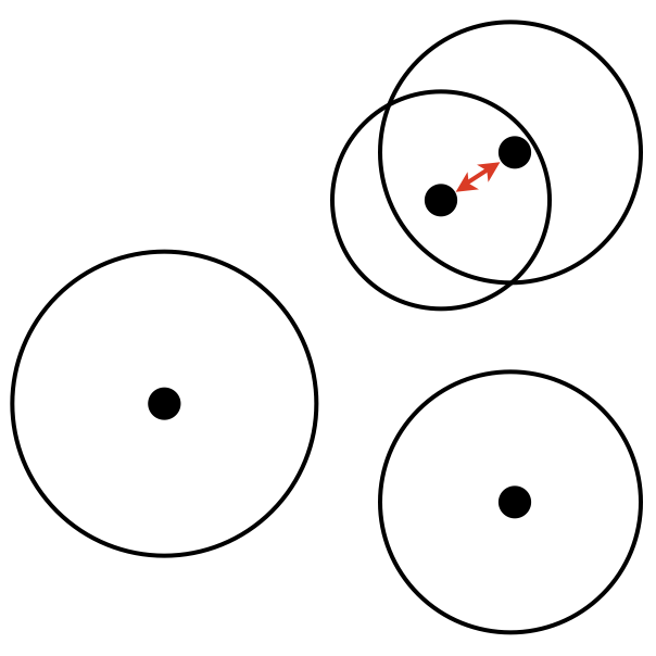
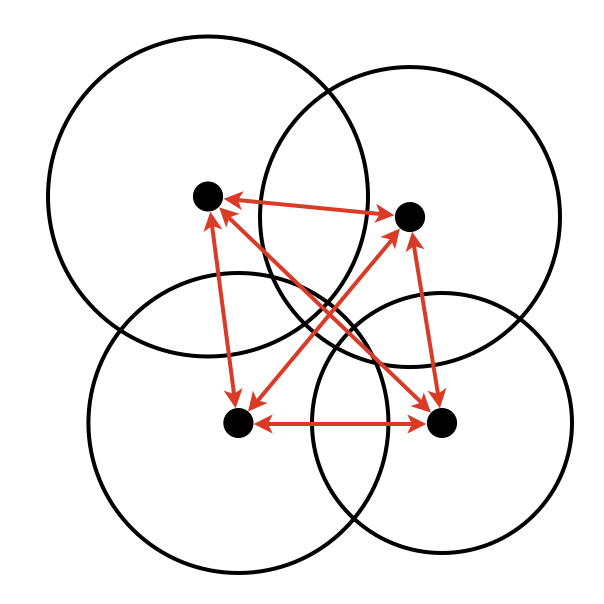
	(a) fully decentralized	(b) partially decentralized	(c) fully centralized
​ [31]	$1/4$	$[1/4,1/2]$	$\color[rgb]{0,0,1}1/2$
​ [32]	$1/4$	$[1/4,1/3]$	$\color[rgb]{0,0,1}1/2$
RAG	$\color[rgb]{0,0,1}1/2$	$\color[rgb]{0,0,1}1/2$	$\color[rgb]{0,0,1}1/2$

Figure 6: Comparison of Suboptimality Guarantees of [31, 32] and RAG: Example of Area Coverage. We make the comparison over an area coverage task with multiple drones, as in Fig. 5(a), where the drones need to each select a short trajectory to maximize the total covered area at the next time step. The stars are the drones’ positions, the circles are the their field-of-views (FOVs), and the red lines denote undirected communication links. The best performances for each metric are colored in blue. (a) The drones are fully decentralized (no inter-agent communication). The bounds by [31, 32] are both $1/4$. For $|{\cal N}|$ agents, instead of $4$, the bounds would be $O(1/|{\cal N}|)$. However, since the drones are far enough for their FOV to overlap, ${\sf coin}_{f,i}=0,\forall i$, and thus RAG can guarantee $1/2$. (b) The drones are partially decentralized such that only the physically close drones communicate. For this communication graph, which we assume to be the same as the information-action access graph, $\omega=2$, $\chi=2$, and $\alpha^{\star}=3$. Therefore, [31] gives $[1/4,1/2]$ and [32] gives $[1/4,1/3]$. RAG still gives $1/2$ since non-neighbors are far away for all drones. (c) In the fully centralized case, all methods give $1/2$. In all, RAG may provide tighter bounds than [31, 32] since it considers the actual function $f$ using ${\sf coin}_{f}$ but [31, 32] are agnostic to $f$.

We summarize the approximation guarantees of the state of the art and of RAG in Table I. Therein, we observe the trade-off of decision time and optimality: the algorithms with the best suboptimality guarantees —first six rows of the table, achieving the near-optimal $1/2$ or $1-1/e$ [16]— can exhibit also the worst decision times, one to two orders higher than that of RAG. We discuss the algorithms’ decision times in more detail in Section VI. Among the remaining algorithms —three last rows of the table— RAG is the only algorithm that provides task-aware ($f$-based) performance guarantees, and that quantifies the suboptimality guarantee as a function of each agent’s local communication network of agents. Instead, the guarantees of [31, 32] are task-agnostic and can scale inversely proportional to the number of agents even when RAG can still guarantee the near-optimal $1/2$, as illustrated in Fig. 6.

To discuss the suboptimality guarantees of [31, 32] in more detail, we present their decision-making rule. Specifically, [31, 32] use the following distributed submodular maximization (DSM) rule, introduced in [31]:

$$a_{i}^{\sf DSM}\,\in\,\max_{a\,\in\,{\cal V}_{i}}\;\;f(\,a\;|\;\{a_{j}^{\sf DSM}\}_{j\,\in\,{\cal N}_{i}^{\text{in}}}\,),$$ (14)

where ${\cal N}_{i}^{\text{in}}\subseteq[i-1]$. Equation 14 generalizes SG’s rule in eq. 4 to the setting where agent $i$ has access only to the actions selected by the agents in ${\cal N}_{i}^{\text{in}}\subseteq[i-1]$, instead of all agents that have selected an action before agent $i$. The information-access structure prescribed by the rule in eq. 14 can be represented as a directed acyclic graph ${\cal G}_{\text{info}}$, where agent $i$’s neighbors in ${\cal G}_{\text{info}}$ are the set ${\cal N}_{i}^{\text{in}}$ of agents. Due to the limited information access, the suboptimality guarantees of [31, 32] take the form presented in Table I, where $\omega({\cal G}_{\text{info}})$ is the clique number of ${\cal G}_{\text{info}}$, $\chi({\cal G}_{\text{info}})$ is the chromatic number, and $\alpha^{\star}({\cal G}_{\text{info}})$ is the fractional independence number [49].

VI Decision Time Analysis

We present the decision time of RAG, that is, the time it takes for RAG to terminate, and provide an approximate solution to 1. RAG’s decision time scales linearly with the size of the network, up to two orders faster than the state-of-the-art algorithms. We summarize the decision time of the state of the art and of RAG in Table I, where we use the notation:

• $\tau_{f}$ is the time required for one evaluation of $f$;

• $\tau_{c}$ is the time for transmitting an action through a communication channel $(i\rightarrow j)\in{\cal E}$;

• $\tau_{\#}$ is the time for transmitting a real number through a communication channel $(i\rightarrow j)\in{\cal E}$; evidently, $\tau_{\#}\ll\tau_{f}$ and $\tau_{\#}\ll\tau_{c}$.

• ${\sf diam}({\cal G})$ is the diameter of a graph ${\cal G}$, i.e., the longest shortest path among any pair of nodes in ${\cal G}$ [50].

We base our analysis on the observation that the decision time of any distributed algorithm depends on the algorithm’s:

• computational complexity, namely, the number of function evaluations required till termination (ignoring addition and multiplications as negligible in comparison); and

• communication complexity, namely, the number of communication rounds needed till termination, accounting for the length of the communication messages per each round.

VI-A Decision Time of RAG

We next first analyze the computational and communication complexities of RAG and then present its decision time.

Proposition 3 (Computational Complexity).

RAG requires each agent $i$ to perform at most $|\mathcal{V}_{i}||\mathcal{N}_{i}|$ function evaluations.

Proof.

For each agent $i$, $|{\cal A}_{i}|$ increases by at least one with each “while loop” iteration of RAG. At each such iteration, agent $i$ needs to perform $|{\cal V}_{i}|$ function evaluations to evaluate its marginal gain of all $v\in\mathcal{V}_{i}$ (lines 3–4). Since $|{\cal A}_{i}|\,\leq|{\cal N}_{i}|$, agent $i$ will perform at most $|{\cal V}_{i}||\mathcal{N}_{i}|$ function evaluations. ∎

Proposition 4 (Communication Complexity).

RAG requires at most $|{\cal N}|-1$ communication rounds where a real number is transmitted, and at most $|{\cal N}|-1$ communication rounds where an action is transmitted.

Proof.

The number of “while loop” iterations of RAG is at most $|\mathcal{N}|-1$ because at each iteration at least one agent will select an action. Besides, each “while loop” iteration includes two communication rounds: one for transmitting a marginal gain value (line 5), and one for transmitting an action (lines 8 and 11). Hence, Proposition 4 holds. ∎

Theorem 3 (Decision Time of RAG).

RAG terminates in at most $(\tau_{c}+\tau_{\#})\,(|{\cal N}|-1)\,+\,\tau_{f}\,\max_{i\,\in\,{\cal N}}\,(|\mathcal{V}_{i}|\,|\mathcal{N}_{i}|)$ time.

Proof.

Theorem 3 holds from Propositions 3 and 4. ∎

VI-B Comparison to the State of the Art

We summarize the decision times of the state of the art and of RAG in Table I. RAG’s decision time scales linearly with the network’s size, namely, $|{\cal N}|$, whereas, in the worst case, the state of the art scales at least quadratically with $|{\cal N}|$. Specifically, RAG has computational time that is linear in $|{\cal N}_{i}|$, independent of $|{\cal N}|$, and communication time linear in $|{\cal N}|$. The comparison is summarized in Table I. Therein, for the sake of the comparison, we assume for simplicity that $|{\cal V}_{i}|\,=\!|{\cal V}_{j}|,\forall i,j\in{\cal N}$. Also, we divide the state of the art into algorithms that solve 1 either indirectly in the continuous domain via employing the multi-linear extension [48] of the set function $f$ [20, 47, 46], or directly in the discrete domain [39, 21, 43, 31, 32]:^,,

Computation time

RAG requires $\tau_{f}\,|{\cal N}_{i}|\,|{\cal V}_{i}|$ computation time. The method in [21] requires computation time $\tau_{f}\,\sum_{i\,\in\,{\cal N}}\,|{\cal V}_{i}|\,=\!\tau_{f}\,|{\cal V}_{i}|\,|{\cal N}|$ since each agent $i$ needs to perform $|{\cal V}_{i}|$ computations and the agents perform the computations sequentially. Given a pre-specified information access prescribed by directed acyclic graph (DAG) ${\cal G}_{\text{info}}$, the methods in [31, 32] also instruct the agents to select actions sequentially leading to a computation time at most $\tau_{f}\,|{\cal V}_{i}|\,|{\cal N}|$. This time excludes the time needed to find the ${\cal G}_{\text{info}}$ given an arbitrary communication graph ${\cal G}$. The method in [39] enables parallelized computation among agents by ignoring certain edges of an initially complete ${\cal G}$, resulting in a computation time of $O(\tau_{f}\,|{\cal V}_{i}|\,/\,\epsilon)\leq\tau_{f}\,|{\cal V}_{i}|\,|{\cal N}|$. Compared to [31, 32], the method in [39] also provides a distributed way to find which edges to ignore such that the suboptimality guarantee is optimized, a process that requires an additional computation time of $O(\tau_{f}\,|\mathcal{V}_{i}|^{2}\,(|\mathcal{N}|-1))$. The remaining algorithms require longer computation times, proportional to $|{\cal N}|^{2}$ or more.

Communication time

RAG requires at most $(\tau_{c}+\tau_{\#})\,(|{\cal N}|-1)$ communication time. In [31, 32], the agents need to communicate over ${\cal G}$ per the pre-specified information-access directed acyclic graph ${\cal G}_{\text{info}}$ per the rule in eq. 14 [31, Remark 3.2]. In Appendix IV, we identify a worst case where this rule results in $O(\tau_{c}\,|{\cal N}|^{2})$ communication time. This happens when each agent $i-1$ and agent $i$ in the decision sequence do not communicate directly, thus, the information of agent $i-1$ needs to be relayed to agent $i$ via other agents that form a connected communication path between the two. The method in [21], which introduces a depth-first search (DFS) procedure to determine the best agents’ ordering to run SG [18] over arbitrary (strongly) connected networks (instead of just line graphs), requires a worst-case communication time of $O(\tau_{c}\,|{\cal N}|^{3})$ for directed networks, and $O(\tau_{c}\,|{\cal N}|^{2})$ for undirected networks [6, Appendix II]. For some $\epsilon$, the method in [39] may require less communication time for running the algorithm per se than other methods, but an additional communication time of $O(\tau_{c}\,|{\cal V}_{i}|)$ is needed to distributively find a DAG that optimizes the algorithm’s approximation performance. The remaining algorithms require communication times proportional to $|{\cal N}|^{2}$ or more.

VII Evaluation in Road Detection and Coverage

We evaluate RAG in two scenarios of simulated experiments of road detection and coverage tasks, one involving 15 and the other 45 robots. In both cases, the robots operate fully as a distributed/mesh network. RAG achieves planning at the order of $1$Hz and has superior coverage performance against the competitive near-optimal algorithms.

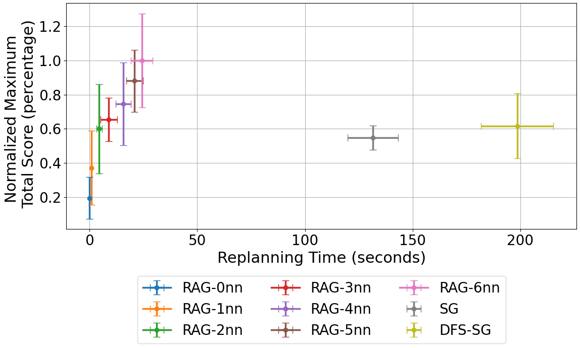
Figure 10: Maximum Total Road-Area Coverage vs. Replanning Time (45 robots). The total road area covered is normalized by the result of RAG-6nn. Team replanning times include ROS1 delays, with a maximum of 5.808 seconds per replanning period.

To perform the evaluations, we extend AirSim [4] to the multi-robot setting, simulating v2v communication delays (Fig. 3). We use ROS1. Thus, the evaluations include ROS1’s inherent time delays due to the transport layer and message passing overhead, as reported in Figs. 7–10.

The code of the simulator will be made available herein.

Common Simulation Setup across Simulated Scenarios. We first define the task of road detection and coverage (Fig. 1), then introduce the compared algorithms, and, finally, present the simulation pipeline (Fig. 3).

Road detection and coverage task

Multiple aerial robots with onboard cameras are deployed in an unknown urban environment and tasked to detect and monitor the roads (Fig. 1). To perform the task, given the currently visible environment, the robots jointly plan how to move per the collaborative autonomy pipeline in Fig. 2. Particularly, the task takes the form of the optimization problem in eq. 1 where $f$ denotes the number of road pixels captured by all robots’ collective FOV after they traverse their planned trajectories $\{a_{i}\}_{i\,\in\,{\cal N}}$ —$f$ is non-decreasing, submodular, and 2nd-order submodular [39]— and ${\cal V}_{i}$ denotes robot $i$’s available trajectories at the current planning step. Specifically, ${\cal V}_{i}$ defines the possible directions that the robot can move in, and the speed the robot can move with. We assume that every robot can move in any of the 8 cardinal directions —N E S W NE SE NW SW— relative to its body frame, for $10$ m at $3$ m/s.

Without loss of generality, the deployed robots are assumed to have the same onboard sensing and communication capabilities: all robots are equipped with (i) an inertial measurement unit (IMU); (ii) a GPS signal receiver; (iii) a downward-facing camera mounted on a gimbal that enables the camera to point to any of the 8 cardinal directions relative to the robot’s body frame; and (iv) a communication module that enables $10$ MByte/s data rate per inter-robot communication channel. Each robot can establish a few communication channels per a specified communication bandwidth constraint, only with those robots that are within $100$ m.

Compared algorithms

Across various bandwidth constraints for the robots, we compare RAG with two competitive near-optimal algorithms: the Sequential Greedy (SG) algorithm [18], also known as Coordinate Descent [1], and its state-of-the-art Depth-First-Search variant (DFS-SG) [21]. Each algorithm is tested in 30 trials, each lasting 2 minutes. In more detail, the setup is as follows:

We test RAG for different bandwidth constraints that vary from $0$ up to $6$. In each case, the same bandwidth constraint applies to all robots. Each such version of RAG is denoted by RAG-$k$nn, where $k=0,\dots,6$. For each $k$, the communication network is determined by having each robot select $k$ nearest other robots as neighbors subject to the $100$ m communication range. If fewer than $k$ others are within the communication range, then all are selected as neighbors.

The SG algorithm requires the robots to be arranged on a line graph that defines the order in which the robots select actions per eq. 4 and enables the information relay from robots that have already selected actions to the robot currently selecting an action. To ensure the existence of a line graph in our simulations of SG, we randomly generate one, adjusting the robots’ communication ranges to infinity.

The DFS-SG algorithm enables SG to be applied to networks that are not necessarily a line graph, but the networks still need to be strongly connected. To this end, we construct strongly connected graphs by first randomly constructing line graphs as for SG, then randomly adding a few undirected edges to the line graphs, particularly, 30 edges for the 15-robot case and 90 edges for the 45-robot case. At each planning round, DFS-SG randomly picks the first robot to select an action, and the order of all other robots is determined by a distributed method based on depth-first search. The resulting decision sequence may involve relay robots that transmit information between robots that are not directly connected and, thus, DFS-SG generally requires longer decision times than SG.

Simulation pipeline

The simulation pipeline consists of the following modules (Fig. 3):

• Network Self-Configuration: This module applies only to RAG since only RAG enables the network to self-configure itself across the planning steps subject to the robots’ bandwidth constraints and the robots’ relative locations. Particularly, as described also in the above paragraph for RAG-$k$nn, at the beginning of each planning step, each robot selects its $k$ nearest other robots within its communication range. This neighborhood selection scheme is justified by Example 1.

• Perception: This process is different for each algorithm since each algorithm requires each robot to process information received from different sets of robots. For RAG, the robots need the following three operations to detect the nearby environment and evaluate where would be best to move: (i) At the beginning of each planning step, each robot hovers at a constant height (30 m) and rotates its camera to take a picture in each of the 8 cardinal directions relative to its body frame. The captured FOV in each direction is of size $34.6\times 26.0$ m². Then, the robot uses semantic segmentation to detect the road segments in each of the 8 captured images. The resulting segmented image has size $1$ MByte. (ii) Each robot, upon receiving segmented images and relative poses from neighbors that have committed actions in specific directions, stitches these images together. That way, the robot reconstructs the collective FOV of its neighbors that have committed an action. This reconstruction will be used next by the robot to select in which direction to move to cover the most new road area. To this end, (iii) the robot stitches its 8 captured images respectively with the previous reconstruction and counts the extra road pixels that can be covered in each of the corresponding 8 cardinal directions.

  For SG and DFS-SG, the operations above are similar, with the modification being that instead of just the neighbors’ segmented and stitched images, each robot leverages all previous robots’ stitched images in (ii) and (iii).

• Action Coordination: This process is different for each algorithm. For RAG, given their neighbors’ already committed actions, the robots that are still deciding will first each pick a trajectory whose FOV gives the most amount of newly covered road area. Then, they will compare this amount with one another. Those who win their neighbors will commit to their picked trajectories and share the corresponding FOV and camera pose with neighbors. Otherwise, they will receive the FOVs and camera poses selected by newly committed robots and repeat the process above.

  For SG, the robots make decisions sequentially in a line graph. Each robot, upon receiving the stitched FOVs of the trajectories selected by all predecessors, will first choose the trajectory whose FOV offers the most newly covered area based on previous robots’ selections. It will then align and stitch this FOV with the received ones, and finally send the newly stitched FOVs to the next robot.

  The coordination process for DFS-SG is similar to SG, with the difference being that DFS-SG operates over a strongly connected network, given the robots’ locations, bandwidth, and communication range, instead of a line graph. Thus, during DFS-SG, the $i$-th robot in the decision sequence may need to transmit FOVs to the $(i+1)$-th robot in the decision sequence via relay robots.

• Control: The robots simultaneously traverse the trajectories after coordination using “simple_flight”, a flight controller in AirSim. “simple_flight” uses cascade PID controllers to drive the aerial robots to move in the selected direction with speed $3.0$ m/s for $10.0$ m.

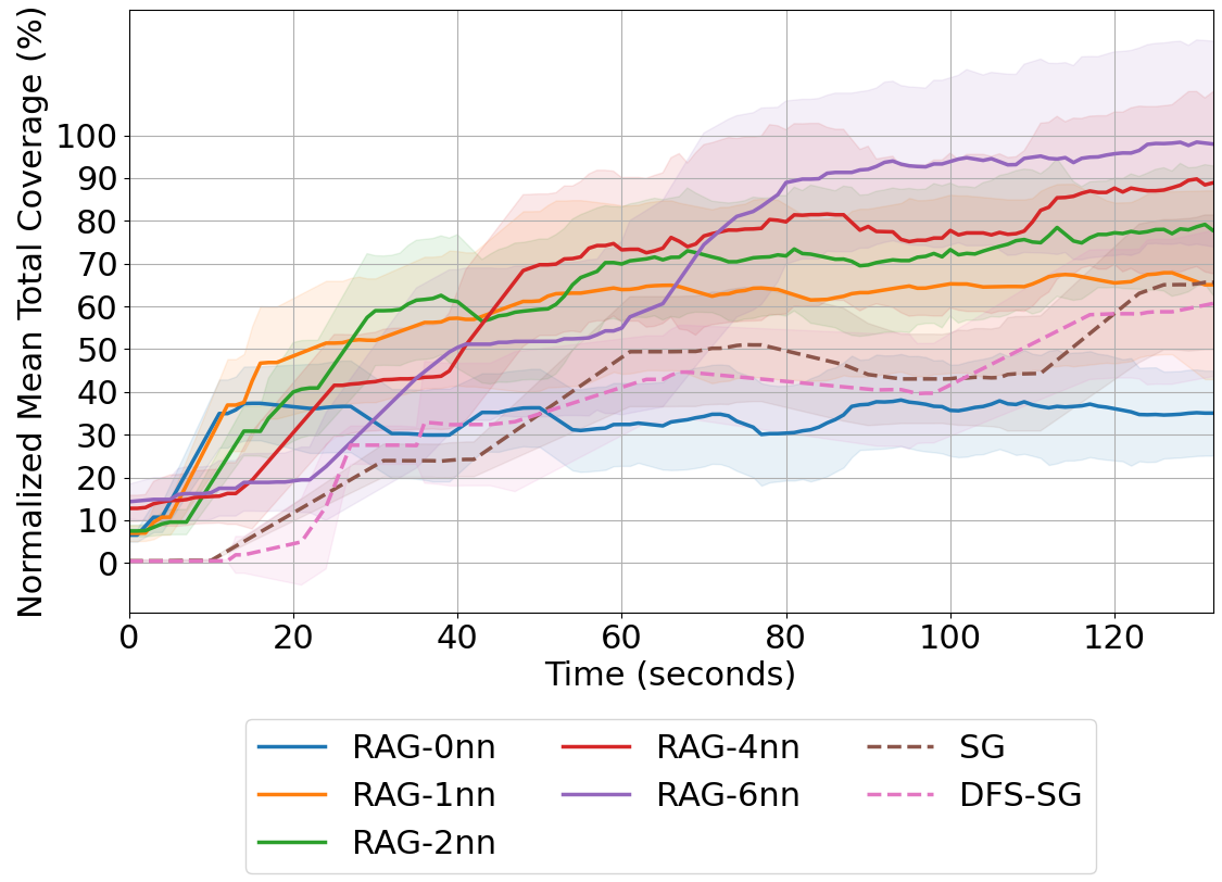
Figure 7: Total Road-Area Coverage vs. Time (15 robots). The total road area covered is normalized by the result of RAG-6nn. The reported time includes ROS1 delays, with a maximum of 1.971 seconds per replanning period.

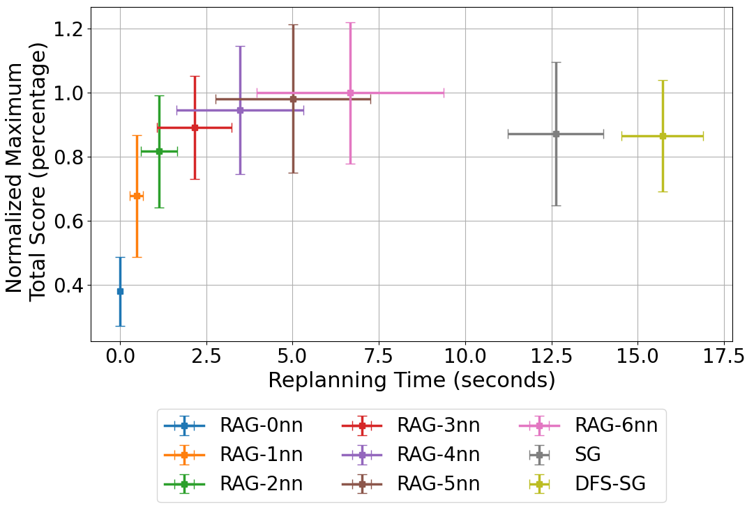
Figure 8: Maximum Total Road-Area Coverage vs. Replanning Time (15 robots). The total road area covered is normalized by the result of RAG-6nn. Team replanning times include ROS1 delays, with a maximum of 1.971 seconds per replanning period.

VII-A Evaluations with 15 Robots

We present the results for the scenario with 15 robots. To this end, we first present in more detail the simulation setup.

Simulation Setup. Across the Monte Carlo tests, the robots are deployed near to one another in a small area such as for the leftmost group in Fig. 1, such that their FOVs largely overlap.

We ran the simulations on a 32-core CPU with 2 Nvidia RTX 4090 24GB GPUs and 128GB RAM on Ubuntu 18.04.

Results. The results are summarized in Figs. 7 and 8. We observe that RAG achieves real-time planning and superior coverage. We also observe that a smaller neighborhood in favor of higher decision efficiency results in only a diminishing impact on the coverage performance. These observations validate the theoretical observation in Remarks 7 and 8.

Coverage performance over time

In Fig. 7, we present the total road area covered across time for each of the compared algorithms. We observe that RAG-$k$nn achieves in all but one case of $k$ ($k=0$) superior performance, one to two orders faster. For example, RAG-$1$nn achieves the same performance at $t=40$ sec as SG and DFS-SG do at $t=140$ sec. The lower final performance for $k=0$ is expected since then there is no coordination. Nevertheless, for the first $10$ to $20$ sec, RAG-$0$nn achieves better coverage since no coordination enables higher replanning frequency.

The reason that the algorithms SG and DFS-SG underperform is that they require more time to terminate per planning step, therefore, over the allocated $120$ sec, the robots replan fewer times in comparison to RAG.

Coverage vs. replanning time

In Fig. 8, we plot the total road area covered by the end of the simulation period ($130$ sec) vs. the average replanning time. We observe that when the neighborhood size for RAG increases, the covered road area increases, as the replanning time also does. This is expected since larger neighborhoods imply more coordination, thus better coverage performance but slower pace.

Smaller neighborhoods can be enough

In Fig. 8, we observe diminishing returns in coverage performance as the neighborhood size increases: although the total road area covered increases significantly from $k$ to $k+1$ for $k=0,1,2,4$, it increases marginally for higher $k$. Therefore, centralizing coordination beyond a size of neighborhoods $k=4$ appears inefficient: RAG-4nn seems to balance the trade-off of total coverage and decision speed, enjoying both fast replanning ($3.3$ sec) and high coverage rate (95%): RAG-4nn achieves 95% coverage at $1/3$ of the replanning time of RAG-6nn.

The observation validates the theory that decision speed increases proportionally with the size of the network (Theorem 3) but the total utility sublinearly (Proposition 2).

VII-B Experiments with 45 Drones

We demonstrate the scalability of our algorithm from 15 to 45 robots. We show that RAG maintains similar decision time and coverage as for the 15-robot setting, being at most 2 times slower, due to enabling parallelized decision-making. In contrast, the compared algorithms now require $2$ to $3$ minutes per replanning step instead of $12$ seconds, a $15$ times increase. By executing the experiments, we also demonstrate that the provided simulator pipeline can support such large-scale multi-robot scenarios.

Simulation Setup. Across the Monte Carlo tests, the robots are divided into three groups, with the robots within each group being deployed near to one another such that their FOVs largely overlap (Fig. 1). In such a setting, RAG automatically enables parallelized decision-making, maintaining similar decision time and coverage as for the 15-robot setting, in contrast to the state-of-the-art near-optimal algorithms.

We ran the simulations on a remote server with 80 CPU cores (4x 2.4 GHz Intel Xeon Gold 6148), 360GB RAM, and 4 NVIDIA Tesla V100 16GB GPU.

Results. The results are summarized in Figs. 9 and 10. We observe that RAG still maintains real-time planning and superior coverage, with all qualitative observations from the 15-robot setting applying also here. The near-optimal algorithms now require on average $2$ to $3$ minutes per replanning step, a $15$ times increase compared to the 15-robot case, as expected due to their superlinear time complexity (Table I).

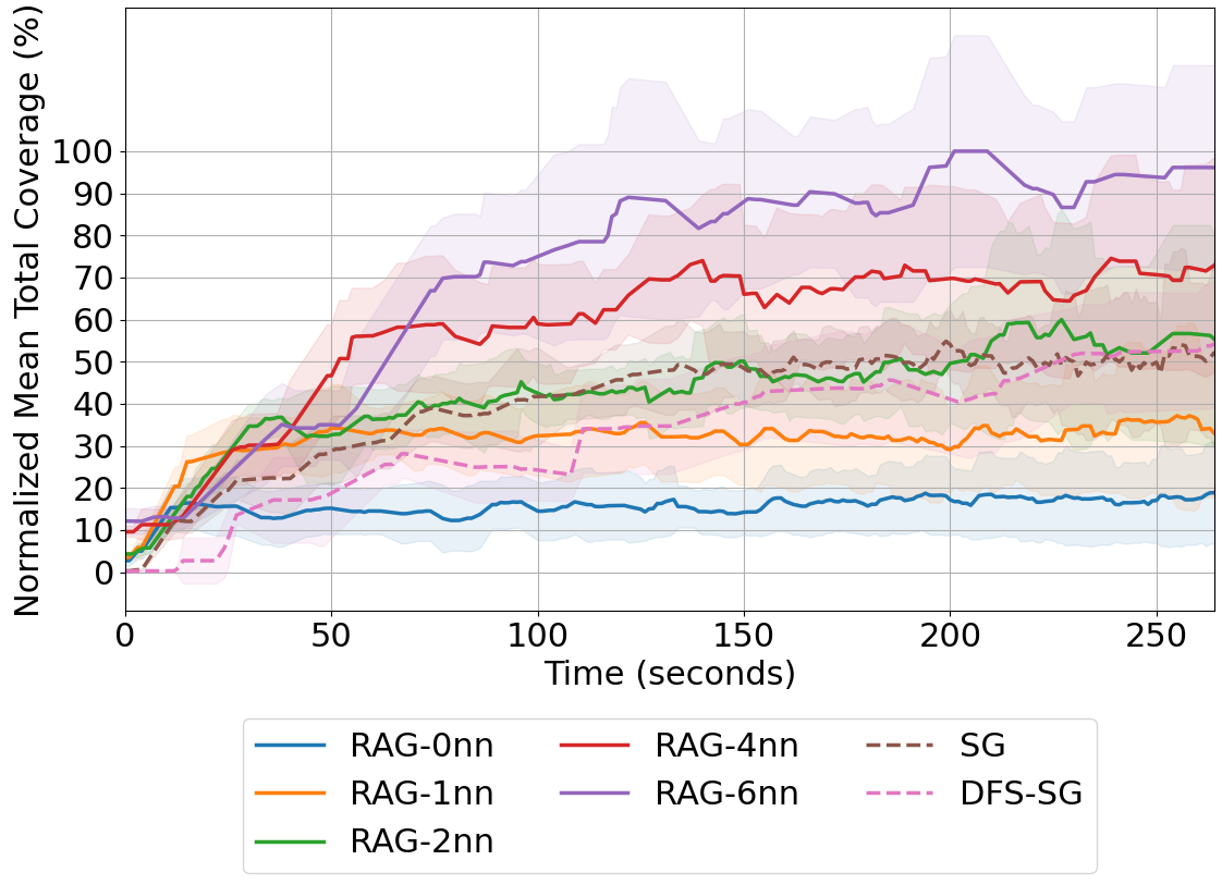
Figure 9: Total Road-Area Coverage vs. Time (45 robots). The total road area covered is normalized by the result of RAG-6nn. The reported time includes ROS1 delays, with a maximum of 5.808 seconds per replanning period.

VIII Conclusion and Future Work

Summary. We provided a rigorous coordination algorithm that enables teams of distributed mobile robots to self-configure their communication topology to achieve real-time and near-optimal coordination. Our coordination paradigm is in contrast to the current paradigms that are either near-optimal but impractical for replanning times or real-time but offer no near-optimality guarantees. We made theoretical and algorithmic contributions to characterize and balance this trade-off between decision speed and optimality. On the theoretical side, we provided an analysis of how the network topology at the robot level —each robot’s coordination neighborhood— affects the near-optimality of the coordination at the global level. On the algorithmic side, we provided a communication- and computation-efficient algorithm that enables the agents to balance the trade-off. Our algorithm is up to two orders faster than competitive near-optimal algorithms. In realistic simulations of surveillance tasks with up to 45 robots, the algorithm enabled real-time planning at the order of $1$ Hz and superior coverage performance. To enable realistic simulations, we provided a high-fidelity simulator that extends the AirSim simulator to integrate a collaborative autonomy pipeline and simulate v2v communication delays.

Future Work. We will enhance our results in three directions. (i) RAG assumes synchronous communication. Although RAG can be trivially modified to handle such cases, e.g., by instructing each robot to execute its action without first waiting for all other robots to select actions, its near-optimality guarantees provided in this paper may become invalid. Our future work will extend our theoretical and algorithmic analysis beyond the above limitations. (ii) We will also extend our results to handle effective task execution over long time horizons. For example, in collaborative mapping over long time horizons, the team needs to stay updated on the areas that have been mapped, such that the current plans do not repeat past actions. This is in addition to the focus of this paper that only the current plans among the robots do not overlap. To this end, we may need also to handle network connectivity constraints over the time horizon. (iii) Finally, we will enhance our simulator by integrating the simulation of realistic communication channels and protocols towards communication-aware and -efficient coordination algorithms.

Appendix I

Proof of Proposition 1

Consider robot $i\in{\cal N}$ and two disjoint robot sets ${\cal B}_{1},{\cal B}_{2}\subseteq{\cal N}\setminus\{i\}$, we have

$${\sf coin}_{f,i}({\cal B}_{1}\cup{\cal B}_{2})-{\sf coin}_{f,i}({\cal B}_{1})$$

$$=f(a_{i}\,|\,\{a_{j}\}_{j\,\in\,{\cal B}_{1}\cup{\cal B}_{2}})-f(a_{i}\,|\,\{a_{j}\}_{j\,\in\,{\cal B}_{1}})$$ (15)

$$\leq f(a_{i}\,|\,\{a_{j}\}_{j\,\in\,{\cal B}_{1}})-f(a_{i}\,|\,\{a_{j}\}_{j\,\in\,{\cal B}_{1}})=0,$$ (16)

where the inequality holds since $f$ is submodular. Hence, ${\sf coin}_{f,i}({\cal N}_{i})$ is non-increasing in ${\cal N}_{i}$. Therefore, for any $i\in{\cal N}$, ${\sf coin}_{f,i}({\cal N}_{i})$ achieves the lower bound ${\sf coin}_{f,i}({\cal N}_{i})\geq{\sf coin}_{f,i}({\cal N}\setminus\{i\})=f(a_{i})-f(a_{i}\,|\,\emptyset)\geq 0$. For the upper bound,

$${\sf coin}_{f,i}({\cal N}_{i}) \leq{\sf coin}_{f,i}(\emptyset)=f(a_{i})-f(a_{i}\,|\,{\cal A}_{{\cal N}\setminus\{i\}})$$ (17)

$$\leq\kappa_{f}f(a_{i}),$$ (18)

where the first inequality holds since ${\sf coin}_{f,i}$ is non-increasing, and the second inequality holds from eq. 5. ∎

Appendix II

We first prove Theorem 1, and then present and prove the bounds of RAG when $f$ is submodular or approximately submodular instead of 2nd-order submodular.

Proof of Theorem 1

We index each agent in ${\cal N}$ per its selecting order in RAG, i.e., agent $i\in\mathcal{N}\triangleq\{1,\dots,|\mathcal{N}|\}$ is the $i$-th agent to select an action during the execution of RAG. If multiple agents select actions simultaneously, then we index them randomly. We use also the notation:

• ${\cal A}^{{\sf RAG}}_{\cal X}\triangleq\{a^{\sf RAG}_{i}\}_{i\,\in\,{\cal X}}$ for any ${\cal X}\subseteq{\cal N}$, i.e., ${\cal A}^{{\sf RAG}}_{\cal X}$ is the set of actions selected by the agents in ${\cal X}$.

Then we have,

$$f({\cal A}^{\sf OPT})$$

$$\leq f({\cal A}^{\sf OPT}\cup{\cal A}^{{\sf RAG}})$$ (19)

$$=f({\cal A}^{{\sf RAG}})+\sum_{i\,\in\,{\cal N}}\,f(a_{i}^{\sf OPT}\,|\,{\cal A}^{{\sf RAG}}\cup{\cal A}^{\sf OPT}_{[i-1]})$$ (20)

$$\leq f({\cal A}^{{\sf RAG}})+\sum_{i\,\in\,{\cal N}}\,f(a_{i}^{\sf OPT}\,|\,{\cal A}^{{\sf RAG}}_{\mathcal{N}_{i}\cap[i-1]})$$ (21)

$$\leq f({\cal A}^{{\sf RAG}})+\sum_{i\,\in\,{\cal N}}\,f(a_{i}^{\sf RAG}\,|\,{\cal A}^{{\sf RAG}}_{\mathcal{N}_{i}\cap[i-1]})$$ (22)

$$=2f({\cal A}^{{\sf RAG}})+\sum_{i\,\in\,{\cal N}}\,f(a_{i}^{\sf RAG}\,|\,{\cal A}^{{\sf RAG}}_{\mathcal{N}_{i}\cap[i-1]})$$

$$\hskip 142.26378pt-f(a_{i}^{\sf RAG}\,|\,{\cal A}^{{\sf RAG}}_{[i-1]})$$ (23)

$$=2f({\cal A}^{{\sf RAG}})+\sum_{i\,\in\,{\cal N}}\,f(a_{i}^{\sf RAG}\,|\,{\cal A}^{{\sf RAG}}_{\mathcal{N}_{i}\cap[i-1]})$$

$$\quad\quad\quad\quad\quad\quad\quad-f(a_{i}^{\sf RAG}\,|\,{\cal A}^{{\sf RAG}}_{\mathcal{N}_{i}\cap[i-1]}\cup{\cal A}^{{\sf RAG}}_{[i-1]\setminus\mathcal{N}_{i}})$$ (24)

$$\leq 2f({\cal A}^{{\sf RAG}})+\sum_{i\,\in\,{\cal N}}\,f(a_{i}^{\sf RAG})-f(a_{i}^{\sf RAG}\,|\,{\cal A}^{{\sf RAG}}_{[i-1]\setminus\mathcal{N}_{i}})$$ (25)

$$\leq 2f({\cal A}^{{\sf RAG}})+\sum_{i\,\in\,{\cal N}}\,f(a_{i}^{\sf RAG})-f(a_{i}^{\sf RAG}\,|\,{\cal A}^{{\sf RAG}}_{{\cal N}_{i}^{c}})$$ (26)

$$\leq 2f({\cal A}^{{\sf RAG}})+\sum_{i\,\in\,{\cal N}}\,{\sf coin}_{f,i}({\cal N}_{i}),$$ (27)

where eq. 19 holds from the monotonicity of $f$; eqs. 20 and 23 result from telescoping the sums; eqs. 21 and 26 hold from the submodularity of $f$; eq. 22 holds since RAG selects $a^{{\sf RAG}}_{i}$ greedily; eq. 24 holds since ${\cal A}^{{\sf RAG}}_{[i-1]}={\cal A}^{{\sf RAG}}_{\mathcal{N}_{i}\cap[i-1]}\cup{\cal A}^{{\sf RAG}}_{[i-1]\setminus\mathcal{N}_{i}}$; eq. 25 holds from the 2nd-order submodularity of $f$; and eq. 27 holds from Definition 3. Therefore, eq. 9 holds.

Then, in the fully centralized case where ${\cal N}_{i}^{c}=\emptyset,\forall i\in{\cal N}$,

$$f({\cal A}^{\sf OPT}) \leq f({\cal A}^{{\sf RAG}})+\sum_{i\,\in\,{\cal N}}\,f(a_{i}^{\sf RAG}\,|\,{\cal A}^{{\sf RAG}}_{\mathcal{N}_{i}\cap[i-1]})$$ (28)

$$\leq f({\cal A}^{{\sf RAG}})+\sum_{i\,\in\,{\cal N}}\,f(a_{i}^{\sf RAG}\,|\,{\cal A}^{{\sf RAG}}_{[i-1]})$$ (29)

$$=2f({\cal A}^{{\sf RAG}}),$$ (30)

where eq. 28 follows eq. 22, eq. 29 holds since ${\cal N}_{i}={\cal N}\setminus\{i\},\forall i\in{\cal N}$, and eq. 30 holds by telescoping the sums. Thus, eq. 10 is proved.

Alternatively, we can prove eq. 10 with eq. 27 and using ${\sf coin}_{f,i}({\cal N}_{i})=f(a_{i}^{\sf RAG})-f(a_{i}^{\sf RAG})=0$.

Finally, in the fully decentralized case where ${\cal N}_{i}^{c}={\cal N}\setminus\{i\},\forall i\in{\cal N}$, we have

$$\sum_{i\,\in\,{\cal N}}{\sf coin}_{f,i}({\cal N}_{i}) =\sum_{i\,\in\,{\cal N}}f(a_{i}^{\sf RAG})-f(a_{i}^{\sf RAG}\,|\,{\cal A}_{{\cal N}\setminus\{i\}}^{\sf RAG})$$ (31)

$$\leq\kappa_{f}\sum_{i\,\in\,{\cal N}}f(a_{i}^{\sf RAG})$$ (32)

$$\leq\frac{\kappa_{f}}{1-\kappa_{f}}f({\cal A}^{\sf RAG}),$$ (33)

where eq. 32 holds from eq. 5, and eq. 33 holds from [51, Lemma 2.1]. Combining eqs. 27 and 33, the lower bound in eq. 12 can be proved. ∎

Suboptimality Bounds of RAG for Submodular or Approximately Submodular $f$

We present the bounds in Theorem 4. To this end, we use the following definition.

Definition 4 (Total curvature [17, 16]).

Consider $f\colon 2^{\cal V}\mapsto\mathbb{R}$ is non-decreasing. Then, $f$’s total curvature is defined as

$$c_{f}\triangleq 1-\min_{v\,\in\,{\cal V}}\min_{{\cal A},\mathcal{B}\,\subseteq\,{\cal V}\setminus\{v\}}\frac{f(\{v\}\cup{\cal A})-f({\cal A})}{f(\{v\}\cup\mathcal{B})-f(\mathcal{B})}.$$ (34)

Similarly to $\kappa_{f}$, it also is $c_{f}\in[0,1]$. When $f$ is submodular, then $c_{f}=\kappa_{f}$. Generally, if $c_{f}=0$, then $f$ is modular, while if $c_{f}=1$, then eq. (34) implies the assumption that $f$ is non-decreasing. In [52], any monotone $f$ with total curvature $c_{f}$ is called $c_{f}$-submodular, as repeated below.

Theorem 4 (Suboptimality Bounds for Submodular or Approximately Submodular Functions).

${\cal A}^{{\sf RAG}}$ enjoys the following approximation bounds:

• if $f$ is non-decreasing submodular and ${\cal G}$ is fully centralized,

  $$f(\,{\cal A}^{{\sf RAG}}\,)\,\geq\,\frac{1}{2}\,f(\,\mathcal{A}^{\sf OPT}\,);$$ (35)

• if $f$ is non-decreasing submodular and ${\cal G}$ is not fully cent- ralized,

  $$f(\,{\cal A}^{{\sf RAG}}\,)\,\geq\,\frac{1-\kappa_{f}}{2-\kappa_{f}}\,f(\,\mathcal{A}^{\sf OPT}\,);$$ (36)

• if $f$ is non-decreasing and ${\cal G}$ is fully centralized,

  $$f(\,{\cal A}^{{\sf RAG}}\,)\,\geq\,\frac{1-c_{f}}{2-c_{f}}\,f(\,\mathcal{A}^{\sf OPT}\,);$$ (37)

• if $f$ is non-decreasing and ${\cal G}$ is not fully centralized,

  $$f(\,{\cal A}^{{\sf RAG}}\,)\,\geq\,\frac{(1-c_{f})^{2}}{(1-c_{f})^{2}+1}\,f(\,\mathcal{A}^{\sf OPT}\,).$$ (38)

Proof of Theorem 4

We present the proof separately for each case. First, when $f$ is submodular with ${\cal G}$ being fully centralized, RAG has the same $1/2$ bound as in Theorem 1 that follows from eqs. 28, 29 and 30.

When $f$ is submodular, and ${\cal G}$ is not fully centralized, RAG provides the same bound as the lower bound in eq. 12:

$$f({\cal A}^{\sf OPT})$$

$$\leq f({\cal A}^{{\sf RAG}})+\sum_{i\,\in\,{\cal N}}\,f(a_{i}^{\sf RAG}\,|\,{\cal A}^{{\sf RAG}}_{\mathcal{N}_{i}\cap[i-1]})$$ (39)

$$=\frac{2-\kappa_{f}}{1-\kappa_{f}}f({\cal A}^{{\sf RAG}})$$ (40)

$$\quad+\sum_{i\,\in\,{\cal N}}\,\left[f(a_{i}^{\sf RAG}\,|\,{\cal A}^{{\sf RAG}}_{\mathcal{N}_{i}\cap[i-1]})-\frac{1}{1-\kappa_{f}}f(a_{i}^{\sf RAG}\,|\,{\cal A}^{{\sf RAG}}_{[i-1]})\right]$$

$$\leq\frac{2-\kappa_{f}}{1-\kappa_{f}}f({\cal A}^{{\sf RAG}})$$

$$\quad+\sum_{i\,\in\,{\cal N}}\,\left[f(a_{i}^{\sf RAG}\,|\,{\cal A}^{{\sf RAG}}_{\mathcal{N}_{i}\cap[i-1]})-f(a_{i}^{\sf RAG}\,|\,{\cal A}^{{\sf RAG}}_{\mathcal{N}_{i}\cap[i-1]})\right]$$ (41)

$$=\frac{2-\kappa_{f}}{1-\kappa_{f}}f({\cal A}^{{\sf RAG}}),$$ (42)

where eq. 39 follows eq. 22; eq. 40 holds by telescoping the sums; and eq. 41 holds from eq. 5:

$$1-\kappa_{f}\leq\frac{f(\,a_{i}^{\sf RAG}\,|\,{\cal A}_{{\cal N}\setminus\{i\}}^{\sf RAG}\,)}{f(\,a_{i}^{\sf RAG}\,)}\leq\frac{f(\,a_{i}^{\sf RAG}\,|\,{\cal A}_{[i-1]}^{\sf RAG}\,)}{f(\,a_{i}^{\sf RAG}\,|\,{\cal A}_{{\cal N}_{i}\cap[i-1]}^{\sf RAG}\,)}.$$ (43)

When $f$ is non-submodular, and ${\cal G}$ is fully centralized,

$$f({\cal A}^{\sf OPT})$$

$$=f({\cal A}^{{\sf RAG}})+\sum_{i\,\in\,{\cal N}}\,f(a_{i}^{\sf OPT}\,|\,{\cal A}^{{\sf RAG}}\cup{\cal A}^{\sf OPT}_{[i-1]})$$ (44)

$$\leq f({\cal A}^{{\sf RAG}})+\sum_{i\,\in\,{\cal N}}\,\frac{1}{1-c_{f}}f(a_{i}^{\sf OPT}\,|\,{\cal A}^{{\sf RAG}}_{\mathcal{N}_{i}\cap[i-1]})$$ (45)

$$\leq f({\cal A}^{{\sf RAG}})+\sum_{i\,\in\,{\cal N}}\,\frac{1}{1-c_{f}}f(a_{i}^{\sf RAG}\,|\,{\cal A}^{{\sf RAG}}_{\mathcal{N}_{i}\cap[i-1]})$$ (46)

$$=f({\cal A}^{{\sf RAG}})+\sum_{i\,\in\,{\cal N}}\,\frac{1}{1-c_{f}}f(a_{i}^{\sf RAG}\,|\,{\cal A}^{{\sf RAG}}_{[i-1]})$$ (47)

$$=\frac{2-c_{f}}{1-c_{f}}f({\cal A}^{{\sf RAG}}),$$ (48)

where eq. 44 follows from eq. 20, eq. 45 holds from Definition 4, eq. 46 holds since RAG selects $a^{{\sf RAG}}_{i}$ greedily, eq. 47 holds since ${\cal N}_{i}={\cal N}\setminus\{i\}$, and eq. 48 holds by telescoping the sums.

When $f$ is non-submodular, and ${\cal G}$ is not fully centralized,

$$f({\cal A}^{\sf OPT})$$

$$\leq f({\cal A}^{{\sf RAG}})+\sum_{i\,\in\,{\cal N}}\,\frac{1}{1-c_{f}}f(a_{i}^{\sf RAG}\,|\,{\cal A}^{{\sf RAG}}_{\mathcal{N}_{i}\cap[i-1]})$$ (49)

$$=\frac{(1-c_{f})^{2}+1}{(1-c_{f})^{2}}f({\cal A}^{{\sf RAG}})+\sum_{i\,\in\,{\cal N}}\frac{1}{1-c_{f}}f(a_{i}^{\sf RAG}\,|\,{\cal A}^{{\sf RAG}}_{\mathcal{N}_{i}\cap[i-1]})$$

$$\hskip 99.58464pt-\frac{1}{(1-c_{f})^{2}}f(a_{i}^{\sf RAG}\,|\,{\cal A}^{{\sf RAG}}_{[i-1]})$$ (50)

$$\leq\frac{(1-c_{f})^{2}+1}{(1-c_{f})^{2}}f({\cal A}^{{\sf RAG}})+\sum_{i\,\in\,{\cal N}}\frac{1}{(1-c_{f})^{2}}f(a_{i}^{\sf RAG}\,|\,{\cal A}^{{\sf RAG}}_{[i-1]})$$

$$\hskip 99.58464pt-\frac{1}{(1-c_{f})^{2}}f(a_{i}^{\sf RAG}\,|\,{\cal A}^{{\sf RAG}}_{[i-1]})$$ (51)

$$\leq\frac{(1-c_{f})^{2}+1}{(1-c_{f})^{2}}f({\cal A}^{{\sf RAG}}),$$ (52)

where eq. 49 follows eq. 46, eq. 50 holds by telescoping the sums, and Proof of Theorem 4 holds from Definition 4. ∎

Appendix III

We provide the proofs regarding the a posteriori suboptimality bound of RAG.

Proof of Theorem 2

Since ${\cal I}_{i}={\cal N}_{i}\cap[i-1]$, eq. 13 follows eq. 22, and thus Theorem 2 is proved. Notice that $f$ only needs to be submodular instead of 2nd-order submodular for Theorem 2 to hold. ∎

Proof of Proposition 2

Let $\delta_{i}({\cal I}_{i})\triangleq f(\,a_{i}^{({\cal I}_{i})}\,|\,{\cal A}_{{\cal I}_{i}}\,)$, where ${\cal A}_{{\cal I}_{i}}$ is the actions selected by ${\cal I}_{i}$ per RAG, and $a_{i}^{({\cal I}_{i})}$ is the action selected by $i$ per RAG, i.e., greedily. Therefore, proving $\delta_{i}({\cal I}_{i})$ is non-increasing and approximately supermodular in ${\cal I}_{i},\forall i\in{\cal N}$, will be sufficient in proving Proposition 2.

We start with the non-increasing property by proving $\delta_{i}$ is non-increasing. For disjoint sets ${\cal B}_{1},{\cal B}_{2}\subseteq{\cal N}\setminus\{i\}$, we have ${\cal A}_{{\cal B}_{1}}\subseteq{\cal A}_{{\cal B}_{1}\cup{\cal B}_{2}}$ and, thus,

$$\delta_{i}({\cal B}_{1}) =f(\,a_{i}^{({\cal B}_{1})}\,|\,{\cal A}_{{\cal B}_{1}}\,)\geq f(\,a_{i}^{({\cal B}_{1}\cup{\cal B}_{2})}\,|\,{\cal A}_{{\cal B}_{1}}\,)$$ (53)

$$\geq f(\,a_{i}^{({\cal B}_{1}\cup{\cal B}_{2})}\,|\,{\cal A}_{{\cal B}_{1}\cup{\cal B}_{2}}\,)=\delta_{i}({\cal B}_{1}\cup{\cal B}_{2}),$$ (54)

where eq. 53 holds since RAG selects $a_{i}^{({\cal B}_{1})}$ greedily given ${\cal A}_{{\cal B}_{1}}$, and eq. 54 holds since ${\cal A}_{{\cal B}_{1}}\subseteq{\cal A}_{{\cal B}_{1}\cup{\cal B}_{2}}$.

To prove the approximate supermodularity of $\delta_{i}$, we will first prove another function $\delta_{i}^{\prime}$ is supermodular, then show that $\delta_{i}({\cal S})\leq\delta_{i}^{\prime}({\cal S})\leq\delta_{i}({\cal S})+\epsilon,\forall{\cal S}\subseteq{\cal N}\setminus\{i\}$ [57]. In particular, let us define $\delta_{i}^{\prime}({\cal I}_{i})\triangleq f(\,a\,|\,{\cal A}_{{\cal I}_{i}}\,)$, where ${\cal A}_{{\cal I}_{i}}$ is the actions selected per RAG by ${\cal I}_{i}$ as in the definition of $\delta_{i}$, but $a\in{\cal V}_{i}$ is an arbitrary fixed action. Consider robot set ${\cal S}\subseteq{\cal N}\setminus\{i\}$ other than ${\cal B}_{1},{\cal B}_{2}$, then

$$\delta_{i}^{\prime}({\cal S}\,|\,{\cal B}_{1})-\delta_{i}^{\prime}({\cal S}\,|\,{\cal B}_{1}\cup{\cal B}_{2})$$ (55)

$$=\delta_{i}^{\prime}({\cal S}\cup{\cal B}_{1})-\delta_{i}^{\prime}({\cal B}_{1})-\delta_{i}^{\prime}({\cal S}\cup{\cal B}_{1}\cup{\cal B}_{2})+\delta_{i}^{\prime}({\cal B}_{1}\cup{\cal B}_{2})$$ (56)

$$=f(\,a\,|\,{\cal A}_{{\cal S}\cup{\cal B}_{1}}\,)-f(\,a\,|\,{\cal A}_{{\cal B}_{1}}\,)$$

$$\quad-f(\,a\,|\,{\cal A}_{{\cal S}\cup{\cal B}_{1}\cup{\cal B}_{2}}\,)+f(\,a\,|\,{\cal A}_{{\cal B}_{1}\cup{\cal B}_{2}}\,)$$ (57)

$$=f(\,a\cup{\cal A}_{{\cal S}\cup{\cal B}_{1}}\,)-f(\,{\cal A}_{{\cal S}\cup{\cal B}_{1}}\,)-f(\,a\cup{\cal A}_{{\cal B}_{1}}\,)+f(\,{\cal A}_{{\cal B}_{1}}\,)$$

$$\quad-f(\,a\cup{\cal A}_{{\cal S}\cup{\cal B}_{1}\cup{\cal B}_{2}}\,)+f(\,{\cal A}_{{\cal S}\cup{\cal B}_{1}\cup{\cal B}_{2}}\,)$$

$$\quad+f(\,a\cup{\cal A}_{{\cal B}_{1}\cup{\cal B}_{2}}\,)-f(\,{\cal A}_{{\cal B}_{1}\cup{\cal B}_{2}}\,)$$ (58)

$$=f(\,{\cal A}_{{\cal S}}\,|\,a\cup{\cal A}_{{\cal B}_{1}}\,)-f(\,{\cal A}_{{\cal S}}\,|\,{\cal A}_{{\cal B}_{1}}\,)$$

$$\quad-f(\,{\cal A}_{{\cal S}}\,|\,a\cup{\cal A}_{{\cal B}_{1}\cup{\cal B}_{2}}\,)+f(\,{\cal A}_{{\cal S}}\,|\,{\cal A}_{{\cal B}_{1}\cup{\cal B}_{2}}\,)$$ (59)

$$\leq f(\,{\cal A}_{{\cal S}}\,|\,a\cup{\cal A}_{{\cal B}_{1}}\,)-f(\,{\cal A}_{{\cal S}}\,|\,{\cal A}_{{\cal B}_{1}}\,)$$

$$\quad-f(\,{\cal A}_{{\cal S}}\,|\,a\cup{\cal A}_{{\cal B}_{1}}\,)+f(\,{\cal A}_{{\cal S}}\,|\,{\cal A}_{{\cal B}_{1}}\,)=0,$$ (60)

where the inequality holds since $f$ is 2nd-order submodular. Hence, $\delta_{i}^{\prime}$ is supermodular. Then, we have,

$$\delta_{i}({\cal S})-\delta_{i}^{\prime}({\cal S}) =f(\,a_{i}^{({\cal S})}\,|\,{\cal A}_{{\cal S}}\,)-f(\,a\,|\,{\cal A}_{{\cal S}}\,)$$

$$\leq f(\,a_{i}^{({\cal S})}\,)-(1-\kappa_{f})f(\,a\,),$$ (61)

which holds from the submodularity of $f$ and eq. 5:

$$1-\kappa_{f}\leq\frac{f(\,a\,|\,{\cal A}_{{\cal N}\setminus\{i\}}\,)}{f(\,a\,)}\leq\frac{f(\,a\,|\,{\cal A}_{{\cal S}}\,)}{f(\,a\,)}.$$ (62)

Also, $\delta_{i}({\cal S})-\delta_{i}^{\prime}({\cal S})\geq f(\,a_{i}^{({\cal S})}\,|\,{\cal A}_{{\cal S}}\,)-f(\,a_{i}^{({\cal S})}\,|\,{\cal A}_{{\cal S}}\,)=0$ since RAG selects $a_{i}^{({\cal S})}$ greedily. All in all, $\delta_{i}^{\prime}({\cal S})\leq\delta_{i}({\cal S})\leq\delta_{i}^{\prime}({\cal S})+\epsilon$ holds true with

$$\epsilon=\min_{a_{2}\,\in\,{\cal V}_{i}}\max_{a_{1}\,\in\,{\cal V}_{i}}\;\left[f(\,a_{1}\,)-(1-\kappa_{f})f(\,a_{2}\,)\right],$$ (63)

that is, $\delta_{i}$ is approximately supermodular. ∎

Appendix IV

We provide the proof of the communication time of the algorithm in [31, 32]: the worst-case communication time of the two methods occurs when, for example, if the informational DAG ${\cal G}^{\prime}$ is complete, i.e., each agent $i$ requires information from $[i-1]$, then

• for undirected graphs ${\cal G}$, e.g., when agent $1$ locates in the center of a line graph and the rest are ordered alternately extending outward from the center to both ends of the line (e.g., $5\leftrightarrow 3\leftrightarrow 1\leftrightarrow 2\leftrightarrow 4\leftrightarrow 6$), which leads to $\sum_{i=1}^{|{\cal N}|-1}\tau_{c}\times i=1/2\,\tau_{c}\,|{\cal N}|\,(|{\cal N}|-1)$;

• for directed graphs ${\cal G}$, e.g., when ${\cal G}$ is a one-directional circlic graph yet the agents’ order increases in the other direction (Figure 11), and every agent $i$ needs to traverse all other agents to send information to $i+1$, which leads to $\sum_{i=1}^{|{\cal N}|-1}\tau_{c}\times(|{\cal N}|-2)=\tau_{c}\,(|{\cal N}|-1)(|{\cal N}|-2)$.

Therefore, the worst-case communication time is $O(\tau_{c}\,|{\cal N}|^{2})$ for both undirected and directed ${\cal G}$.

Figure 11: Example of a directed communication graph with the worst-case agent order where each message needs to traverse $|{\cal N}|-2$ edges.

References

- [1] N. Atanasov, J. Le Ny, K. Daniilidis, and G. J. Pappas, “Decentralized active information acquisition: Theory and application to multi-robot SLAM,” in IEEE Inter. Conf. Rob. Auto. (ICRA), 2015, pp. 4775–4782.
- [2] P. Dames, P. Tokekar, and V. Kumar, “Detecting, localizing, and tracking an unknown number of moving targets using a team of mobile robots,” The International Journal of Robotics Research (IJRR), vol. 36, no. 13-14, pp. 1540–1553, 2017.
- [3] M. Corah and N. Michael, “Distributed matroid-constrained submodular maximization for multi-robot exploration: Theory and practice,” Autonomous Robots (AURO), vol. 43, no. 2, pp. 485–501, 2019.
- [4] S. Shah, D. Dey, C. Lovett, and A. Kapoor, “Airsim: High-fidelity visual and physical simulation for autonomous vehicles,” in Field and Service Robotics: Results of the 11th International Conference. Springer, 2018, pp. 621–635.
- [5] Z. Xu and V. Tzoumas, “Resource-aware distributed submodular maximization: A paradigm for multi-robot decision-making,” in IEEE Conference on Decision and Control (CDC), 2022, pp. 5959–5966.
- [6] ——, “Performance-aware self-configurable multi-agent networks: A distributed submodular approach for simultaneous coordination and network design,” 2024.
- [7] A. Krause, A. Singh, and C. Guestrin, “Near-optimal sensor placements in gaussian processes: Theory, efficient algorithms and empirical studies,” Jour. Mach. Learn. Res. (JMLR), vol. 9, pp. 235–284, 2008.
- [8] A. Singh, A. Krause, C. Guestrin, and W. J. Kaiser, “Efficient informative sensing using multiple robots,” Journal of Artificial Intelligence Research (JAIR), vol. 34, pp. 707–755, 2009.
- [9] P. Tokekar, V. Isler, and A. Franchi, “Multi-target visual tracking with aerial robots,” in IEEE/RSJ International Conference on Intelligent Robots and Systems (IROS), 2014, pp. 3067–3072.
- [10] M. Lauri, J. Pajarinen, J. Peters, and S. Frintrop, “Multi-sensor next-best-view planning as matroid-constrained submodular maximization,” IEEE Robotics and Automation Letters (RAL), vol. 5, no. 4, pp. 5323–5330, 2020.
- [11] B. Schlotfeldt, V. Tzoumas, and G. J. Pappas, “Resilient active information acquisition with teams of robots,” IEEE Transactions on Robotics (TRO), vol. 38, no. 1, pp. 244–261, 2021.
- [12] B. Biggs, J. McMahon, P. Baldoni, and D. J. Stilwell, “Non-submodular maximization via the greedy algorithm and the effects of limited information in multi-agent execution,” in IEEE/RSJ International Conference on Intelligent Robots and Systems (IROS), 2022, pp. 10 118–10 125.
- [13] O. Akcin, O. Unuvar, O. Ure, and S. P. Chinchali, “Fleet active learning: A submodular maximization approach,” in 7th Annual Conference on Robot Learning (CoRL), 2023.
- [14] X. Cai, B. Schlotfeldt, K. Khosoussi, N. Atanasov, G. J. Pappas, and J. P. How, “Energy-aware, collision-free information gathering for heterogeneous robot teams,” IEEE Trans. Robotics (TRO), 2023.
- [15] U. Feige, “A threshold of for approximating set cover,” Journal of the ACM (JACM), vol. 45, no. 4, pp. 634–652, 1998.
- [16] M. Sviridenko, J. Vondrák, and J. Ward, “Optimal approximation for submodular and supermodular optimization with bounded curvature,” Math. of Operations Research, vol. 42, no. 4, pp. 1197–1218, 2017.
- [17] ——, “Optimal approximation for submodular and supermodular optimization with bounded curvature,” arXiv preprint:1311.4728, 2013.
- [18] M. L. Fisher, G. L. Nemhauser, and L. A. Wolsey, “An analysis of approximations for maximizing submodular set functions–II,” in Polyhedral combinatorics, 1978, pp. 73–87.
- [19] Q. Wu, J. Xu, Y. Zeng, D. W. K. Ng, N. Al-Dhahir, R. Schober, and A. L. Swindlehurst, “A comprehensive overview on 5G-and-beyond networks with UAVs: From communications to sensing and intelligence,” IEEE Journal on Selected Areas in Communications, vol. 39, no. 10, pp. 2912–2945, 2021.
- [20] A. Robey, A. Adibi, B. Schlotfeldt, H. Hassani, and G. J. Pappas, “Optimal algorithms for submodular maximization with distributed constraints,” in Learn. for Dyn. & Cont. (L4DC), 2021, pp. 150–162.
- [21] R. Konda, D. Grimsman, and J. R. Marden, “Execution order matters in greedy algorithms with limited information,” in American Control Conference (ACC), 2022, pp. 1305–1310.
- [22] B. Yamauchi, “Decentralized coordination for multirobot exploration,” Robotics and Autonomous Systems, vol. 29, no. 2-3, pp. 111–118, 1999.
- [23] R. Zlot, A. Stentz, M. B. Dias, and S. Thayer, “Multi-robot exploration controlled by a market economy,” in IEEE International Conference on Robotics and Automation (ICRA), vol. 3, 2002, pp. 3016–3023.
- [24] M. Berhault, H. Huang, P. Keskinocak, S. Koenig, W. Elmaghraby, P. Griffin, and A. Kleywegt, “Robot exploration with combinatorial auctions,” in IEEE/RSJ International Conference on Intelligent Robots and Systems (IROS), vol. 2, 2003, pp. 1957–1962.
- [25] W. Sheng, Q. Yang, J. Tan, and N. Xi, “Distributed multi-robot coordination in area exploration,” Robotics and Autonomous Systems (RAS), vol. 54, no. 12, pp. 945–955, 2006.
- [26] A. J. Smith and G. A. Hollinger, “Distributed inference-based multi-robot exploration,” Autonomous Robots (AURO), vol. 42, no. 8, pp. 1651–1668, 2018.
- [27] J. Yu, J. Tong, Y. Xu, Z. Xu, H. Dong, T. Yang, and Y. Wang, “Smmr-explore: Submap-based multi-robot exploration system with multi-robot multi-target potential field exploration method,” in IEEE International Conference on Robotics and Automation (ICRA), 2021, pp. 8779–8785.
- [28] Y. Gao, Y. Wang, X. Zhong, T. Yang, M. Wang, Z. Xu, Y. Wang, Y. Lin, C. Xu, and F. Gao, “Meeting-merging-mission: A multi-robot coordinate framework for large-scale communication-limited exploration,” in IEEE/RSJ International Conference on Intelligent Robots and Systems (IROS), 2022, pp. 13 700–13 707.
- [29] L. Klodt and V. Willert, “Equitable workload partitioning for multi-robot exploration through pairwise optimization,” in IEEE/RSJ International Conf. Intelligent Robots and Systems (IROS), 2015, pp. 2809–2816.
- [30] B. Zhou, H. Xu, and S. Shen, “Racer: Rapid collaborative exploration with a decentralized multi-uav system,” IEEE Transactions on Robotics (TRO), 2023.
- [31] B. Gharesifard and S. L. Smith, “Distributed submodular maximization with limited information,” IEEE Transactions on Control of Network Systems (TCNS), vol. 5, no. 4, pp. 1635–1645, 2017.
- [32] D. Grimsman, M. S. Ali, J. P. Hespanha, and J. R. Marden, “The impact of information in distributed submodular maximization,” IEEE Trans. Ctrl. Netw. Sys. (TCNS), vol. 6, no. 4, pp. 1334–1343, 2019.
- [33] F. F. Lizzio, E. Capello, and G. Guglieri, “Implementation and performance evaluation of a consensus protocol for multi-uav formation with communication delay,” in International Conference on Unmanned Aircraft Systems (ICUAS). IEEE, 2022, pp. 1592–1600.
- [34] S. Baidya, Z. Shaikh, and M. Levorato, “FlyNetSim: An open source synchronized UAV network simulator based on NS-3 and ArduPilot,” in Proceedings of the 21st ACM International Conference on Modeling, Analysis and Simulation of Wireless and Mobile Systems, 2018, pp. 37–45.
- [35] M. Calvo-Fullana, D. Mox, A. Pyattaev, J. Fink, V. Kumar, and A. Ribeiro, “Ros-netsim: A framework for the integration of robotic and network simulators,” IEEE Robotics and Automation Letters (RAL), vol. 6, no. 2, pp. 1120–1127, 2021.
- [36] S. Acharya, M. Bharatheesha, Y. Simmhan, and B. Amrutur, “A co-simulation framework for communication and control in autonomous multi-robot systems,” in IEEE/RSJ International Conference on Intelligent Robots and Systems (IROS), 2023, pp. 11 087–11 094.
- [37] M. Selden, J. Zhou, F. Campos, N. Lambert, D. Drew, and K. S. Pister, “BotNet: A simulator for studying the effects of accurate communication models on multi-agent and swarm control,” in International Symposium on Multi-Robot and Multi-Agent Systems (MRS), 2021, pp. 101–109.
- [38] O. S. Oubbati, M. Atiquzzaman, P. Lorenz, M. H. Tareque, and M. S. Hossain, “Routing in flying ad hoc networks: Survey, constraints, and future challenge perspectives,” IEEE Access, pp. 81 057–81 105, 2019.
- [39] M. Corah and N. Michael, “Distributed submodular maximization on partition matroids for planning on large sensor networks,” in IEEE Conference on Decision and Control (CDC), 2018, pp. 6792–6799.
- [40] A. Downie, B. Gharesifard, and S. L. Smith, “Submodular maximization with limited function access,” IEEE Trans. Auto. Ctrl. (TAC), 2022.
- [41] Y. Crama, P. L. Hammer, and R. Holzman, “A characterization of a cone of pseudo-boolean functions via supermodularity-type inequalities,” in Quantitative Methoden in den Wirtschaftswissenschaften. Springer, 1989, pp. 53–55.
- [42] S. Foldes and P. L. Hammer, “Submodularity, supermodularity, and higher-order monotonicities of pseudo-boolean functions,” Mathematics of Operations Research, vol. 30, no. 2, pp. 453–461, 2005.
- [43] J. Liu, L. Zhou, P. Tokekar, and R. K. Williams, “Distributed resilient submodular action selection in adversarial environments,” IEEE Robotics and Automation Letters (RAL), vol. 6, no. 3, pp. 5832–5839, 2021.
- [44] M. Conforti and G. Cornuéjols, “Submodular set functions, matroids and the greedy algorithm,” Discrete Applied Mathematics, vol. 7, no. 3, pp. 251 – 274, 1984.
- [45] T. M. Cover and J. A. Thomas, Elements of Information Theory. John Wiley & Sons, 2012.
- [46] N. Rezazadeh and S. S. Kia, “Distributed strategy selection: A submodular set function maximization approach,” Automatica, vol. 153, p. 111000, 2023.
- [47] B. Du, K. Qian, C. Claudel, and D. Sun, “Jacobi-style iteration for distributed submodular maximization,” IEEE Transactions on Automatic Control (TAC), vol. 67, no. 9, pp. 4687–4702, 2022.
- [48] G. Calinescu, C. Chekuri, M. Pál, and J. Vondrák, “Maximizing a monotone submodular function subject to a matroid constraint,” SIAM Journal on Computing, vol. 40, no. 6, pp. 1740–1766, 2011.
- [49] C. Godsil and G. F. Royle, Algebraic graph theory. Springer Science & Business Media, 2001, vol. 207.
- [50] M. Mesbahi and M. Egerstedt, Graph Theoretic Methods in Multiagent Networks. Princeton University Press, 2010.
- [51] R. K. Iyer, S. Jegelka, and J. A. Bilmes, “Curvature and optimal algorithms for learning and minimizing submodular functions,” in Advances in Neural Inform. Processing Systems (NeurIPS), 2013, pp. 2742–2750.
- [52] B. Lehmann, D. Lehmann, and N. Nisan, “Combinatorial auctions with decreasing marginal utilities,” Games and Economic Behavior, vol. 55, no. 2, pp. 270–296, 2006.
- [53] A. Krause and V. Cevher, “Submodular dictionary selection for sparse representation,” in International Conference on Machine Learning, 2010.
- [54] E. R. Elenberg, R. Khanna, A. G. Dimakis, S. Negahban et al., “Restricted strong convexity implies weak submodularity,” The Annals of Statistics, vol. 46, no. 6B, pp. 3539–3568, 2018.
- [55] L. F. Chamon and A. Ribeiro, “Near-optimality of greedy set selection in the sampling of graph signals,” in IEEE Global Conference on Signal and Information Processing, 2016, pp. 1265–1269.
- [56] B. Guo, O. Karaca, T. Summers, and M. Kamgarpour, “Actuator placement for optimizing network performance under controllability constraints,” in IEEE Conference on Decision and Control (CDC), 2019, pp. 7140–7147.
- [57] T. Horel and Y. Singer, “Maximization of approximately submodular functions,” Advances in Neural Information Processing Systems (NeurIPS), vol. 29, 2016.