Accessing Vision Foundation Models
at ImageNet-level Costs

Abstract

Vision foundation models are renowned for their generalization ability due to massive training data. Nevertheless, they demand tremendous training resources, and the training data is often inaccessible, e.g., CLIP, DINOv2, posing great challenges to developing derivatives that could advance research in this field. In this work, we offer a very simple and general solution, named Proteus, to distill foundation models into smaller equivalents on ImageNet-1K without access to the original training data. Specifically, we remove the designs from conventional knowledge distillation settings that result in dataset bias and present three levels of training objectives, i.e., token, patch, and feature, to maximize the efficacy of knowledge transfer. In this manner, Proteus is trained at ImageNet-level costs with surprising ability, facilitating the accessibility of training foundation models for the broader research community. Leveraging DINOv2-g/14 as the teacher, Proteus-L/14 matches the performance of the Oracle method DINOv2-L/14 (142M training data) across 15 benchmarks and outperforms other vision foundation models including CLIP-L/14 (400M), OpenCLIP-L/14 (400M/2B) and SynCLR-L/14 (600M). Code is available at here.

1 Introduction

By leveraging extensive pre-training on diverse and massive datasets, vision foundation models [43, 54, 46, 11] represent a significant advancement in the field of computer vision, aiming to learn comprehensive and versatile visual features that can generalize well across various downstream tasks, such as classification, segmentation, etc. As a result, vision foundation models are becoming fundamental components in the toolkit of modern computer vision research and development.

While those models have released their weights for public usage, training foundation models remains largely inaccessible for most researchers due to two primary factors: (1) the training data for these foundation models is seldom disclosed. While there have been attempts to reproduce CLIP [46] using alternative datasets [11], replicating the training of foundation models like DINOv2 [43] and SynCLR [54] remains less explored due to private data sources. (2) even if the training data were accessible, training on these enormous datasets necessitates substantial computational resources, which may be beyond the reach of most researchers. ImageNet-1K [13], which has long been the cornerstone for advancements in the supervised learning domain, is now less frequently utilized as a training set in the era of foundation models due to its relatively ‘small’ scale. In this work, we seek to address the following question: Can the success of vision foundation models be replicated on much smaller datasets, such as ImageNet-1K, without sacrificing their generalization ability?

Intuitively, leveraging the pre-trained weights of these foundation models is essential to accomplish this task and there are two possible directions: (1) recent advances [38, 66] in Natural Language Processing (NLP) have validated that structure pruning could be a possible answer as it inherits most of the knowledge from the foundation model. However, they either sample subsets from the original enormous training set [66] or utilize high-quality, representative datasets [38] such as Alpaca [53], making it difficult to trace the success back due to the limited dataset availability in computer vision. More importantly, structure pruning requires delicate hand-crafted designs and cannot be easily generalized to arbitrary architectures, making it challenging to meet the diverse needs of real-world scenarios. (2) TinyCLIP [65] leverages knowledge distillation to transfer the fruitful knowledge from the foundation model CLIP [46] to a customized structure. Although showing great generalization ability across various datasets, it still requires the original large-scale dataset LAION-400M [49] to perform task-agnostic distillation, necessitating extensive training resources and consumption. In pursuit of a more general design, we adventurously choose knowledge distillation as the means to achieve this objective, i.e., transferring the fruitful knowledge embedded in the foundation model to a randomly initialized student network.

There remain two critical issues for the knowledge transfer on ImageNet-1K: (1) the exact distributions of those undisclosed datasets, e.g., WIT400M [46], LVD-142M [43] and SynCaps-150M [54], are unknown and it is likely that a distribution shift exists between ImageNet-1K and these large-scale datasets. This poses significant challenges to the generalization ability of the target model, as the network tends to memorize the training images in a fixed pattern, leading to dataset bias [58, 57, 35]. (2) most vision foundation models [43, 46, 54] are trained with self-supervised learning objectives, which require large amounts of data to be effective. Consequently, directly adopting their optimization strategies may not yield optimal results in our context.

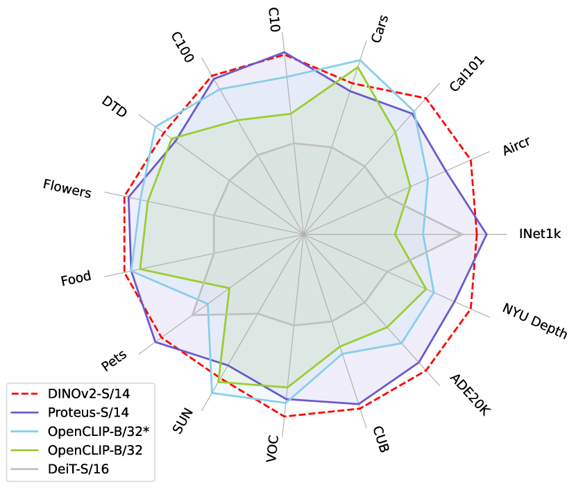
Figure 1: Distilling from DINOv2-B/14 with 1.2M images, Proteus-S/14 outperforms OpenCLIP-B/32 (400M/2B*) on the average performance of 15 benchmarks and falls slightly behind DINOv2-S/14. Each axis is scaled to [0.45, 0.9] for better visualization.

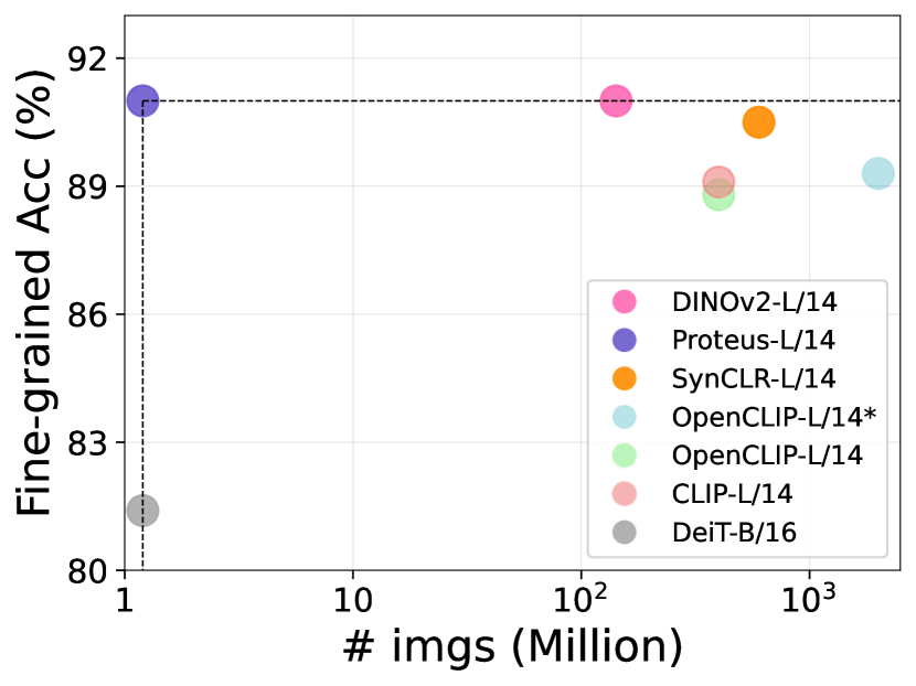
Figure 2: Relationship between the number of training images and average accuracy in 12 fine-grained classification datasets. Distilling from DINOv2-g/14, Proteus-L/14 outperforms OpenCLIP-L/14* (2B) using 0.06$\%$ of its training data and matches the performance of the Oracle model DINOv2-L/14. The X-axis is on a logarithmic scale.

To address the aforementioned challenges, we present Proteus, a simple and general distillation framework to transfer the fruitful knowledge from vision foundation models by emulating their behaviors. We first combat dataset bias and find the introduction of one-hot labels and the projection head in the conventional knowledge distillation setting [26, 59] will lead to dataset bias. Consequently, we perform distillation on the intermediate features [1] and discard the labels. To maximize the knowledge transfer power between the foundation model and the target network, we construct the proxy task by combining the token-level, patch-level, and feature-level learning objectives to learn the general-purpose visual representations, ensuring the performance of Proteus across various tasks.

When leveraging DINOv2-B/14 [43] as the teacher model, Proteus-S/14 exhibits strong generalization ability across 15 benchmarks with 1.2M training images (shown in Fig. 2), which cover the tasks of classification, semantic segmentation, and depth estimation. When scaling up the model size (shown in Fig. 2), Proteus-L/14 matches the performance of the Oracle method DINOv2-L/14 (142M training data) and outperforms other vision foundation models including CLIP-L/14 (400M) [46], OpenCLIP-L/14 (400M/2B*) [11] and SynCLR-L/14 (600M) [54]. Moreover, we obtain significant improvement over the supervised training method DeiT [59] on all metrics using the same training set, promising the potential of Proteus serving as a new training paradigm for supervised learning approaches. Due to the simple but effective design, Proteus can easily generalize to existing vision foundation models to access them at much smaller costs and its generalization ability is verified by accessing SynCLR which is trained on undisclosed 600M synthetic images and CLIP which is trained on WIT-400M. We also provide abundant analysis to share the insights with the research community.

Figure 3: PCA visualization. DINOv2-B/14 is distilled from DINOv2-g on LVD-142M and Proteus-B/14 is distilled from DINOv2-L on ImageNet-1K. Details can be found in Sec. A.10.

2 Methodology

In this section, we present Proteus, a simple and general framework to access vision foundation models with ‘limited’ data, i.e., ImageNet-1K. We first introduce our efforts in mitigating the dataset bias of the proxy dataset so that Proteus can effectively transfer the general representation from the pre-trained foundation models by mimicking its behaviors. Then, we present our proxy task which encompasses multiple levels of learning objectives to promise the applications on various tasks.

2.1 Proxy Dataset

While we do not introduce any new dataset to try to reproduce the results of foundation models [11], we focus on leveraging publicly available resources, e.g., ImageNet-1K, to access the vision foundation models. This task is challenging because the distribution of the large-scale datasets of those foundation models is usually unknown and it is very likely that there exists distribution shifts between ImageNet-1K and those private datasets. Hence, it is critical to reduce the dataset bias [58] of ImageNet-1K so that our learned representation can be general enough.

Combating Dataset Bias. Given a pre-trained teacher network ${F}^{\prime}\left(\cdot\right)$, a foundation model in our context, conventional knowledge distillation [26, 59] optimizes the student network $F\left(\cdot\right)$ by two loss terms. The first one is Cross-Entropy loss which is calculated on the logits of student network $p$:

$$\mathcal{L}_{CE}=-\sum_{k=1}^{K}\hat{y}_{k}\log\left(p_{k}\right),$$ (1)

where $\hat{y}_{k}$ is the one-hot label for class $k$ and $K$ denotes the number of total classes. While the second one is KL divergence loss [31] which enforces the prediction of student network $p$ and teacher model ${p}^{\prime}$ to be as similar as possible:

$$\mathcal{L}_{KL}=-\sum_{k=1}^{K}{p_{k}}^{\prime}\log\left(\frac{p_{k}}{{p_{k}}^{\prime}}\right).$$ (2)

Combining the two losses uniformly, the student network $F\left(\cdot\right)$ can be updated by:

$$\mathcal{L}=\left(1-\lambda\right)\cdot\mathcal{L}_{CE}+\lambda\cdot\mathcal{L}_{KL},$$ (3)

where $\lambda$ is a hyperparameter introduced to balance the two terms. Empirically, the default setting works well in the supervised learning setting as it delivers good performance on ImageNet-1K.

However, we argue that this setup will hinder the knowledge transfer for two reasons: (1) The Cross-Entropy (CE) loss, which leverages the information of one-hot labels, can lead to dataset bias as the model tends to memorize the training images and classes. This memorization makes it challenging for the model to generalize to unseen classes during downstream evaluation. (2) The generation of class logits $p$ implicitly introduces dataset bias because the intermediate features are projected onto a pre-defined dimensionality, such as 1000 for ImageNet-1K, which may be discarded during downstream evaluation. Based on these concerns, we perform knowledge distillation before the project head (FC layer) and leverage the intermediate feature $v$ for knowledge transfer [1].

2.2 Proxy Task

Foundation models such as DINOv2 [43] are designed to learn general-purpose visual features, excelling not only in high-level classification tasks but also in dense prediction tasks like semantic segmentation. To maximize the knowledge transfer power and promise the application on various tasks, we conduct distillation across three different levels of training objectives, i.e., token-level, patch-level, and feature-level, to transfer the fruitful knowledge by emulating the teacher’s behaviors.

Token-level Objective. To learn the discriminative features for high-level understanding, we minimize the L2 distance to align the classification token between the teacher and student model. Specifically, the student classification token $v^{\texttt{cls}}$ will first be mapped to a higher dimension to match the channel number of the teacher’s classification token ${v}^{\prime\texttt{cls}}$:

$$\hat{v}^{\texttt{cls}}=P^{\texttt{cls}}\left(v^{\texttt{cls}}\right),$$ (4)

where $P^{cls}\left(\cdot\right)$ denotes the projection head for the classification token and we simply adopt the combination of Layer Normalization [5] and a linear layer. Then, we enforce the model to mimic the teacher’s prediction ${v}^{\prime\texttt{cls}}$ via Mean Squared Error (MSE) loss:

$$\mathcal{L}_{token}=\|\hat{v}^{\texttt{cls}}-{v}^{\prime\texttt{cls}}\|_{2}^{2}.$$ (5)

Feature-level Objective. Although the token-level learning objective alone serves as a good proxy task to obtain the discriminative visual features, it cannot guarantee decent performance on dense prediction tasks like semantic segmentation or depth estimation (see analysis of Tab. 4.1). To mitigate this issue, we perform feature-level knowledge transfer in a similar manner:

$$\mathcal{L}_{feat}=\|\hat{v}-{v}^{\prime}\|_{2}^{2},$$ (6)

where $\hat{v}$ is obtained by the projection head $P^{feat}\left(\cdot\right)$ for feature distillation.

Patch-level Objective. To further uncover the hidden knowledge from the foundation model, we construct a patch-level learning objective inspired by the idea of masked image modeling [7, 20, 64, 74, 6]. Given an image $x$, an additional view $x_{mask}$ will be generated where the patches are randomly masked and it will be sent to the student network to create the intermediate feature $v_{mask}$. Following the previous procedures, we enforce the student to recover the masked regions by:

$$\mathcal{L}_{patch}=\|\hat{v}_{mask}^{patch}-{v}^{\prime patch}\|_{2}^{2},$$ (7)

where the patch tokens of the foundation model ${v}^{\prime patch}$ is produced by the unmasked view $x$ and $\hat{v}_{mask}^{patch}$ is derived from the projection head $P^{patch}\left(\cdot\right)$.

Combining the three learning objectives, we construct the proxy task of Proteus as follows:

$$\mathcal{L}=\lambda_{token}\cdot\mathcal{L}_{token}+\lambda_{feat}\cdot\mathcal{L}_{feat}+\lambda_{patch}\cdot\mathcal{L}_{patch},$$ (8)

where $\lambda_{token}$, $\lambda_{feat}$, $\lambda_{patch}$ are introduced hyperparameters to balance the three terms and we simply set them to 1 in our implementations without additional fine-tuning.

3 Empirical Validation

In this part, we conduct pre-training on ImageNet-1K [13] and validate our methods under different setups. Distilling from DINOv2 [43], we first evaluate our method on the object recognition task and perform linear probing on ImageNet-1K and 12 fine-grained datasets. Further, we validate our approach on dense prediction tasks, including Semantic Segmentation and Depth Estimation. Moreover, we examine the scaling behavior of our method by switching backbones with different model capacities. In the end, we test the generalization ability of our method by distilling SynCLR [54] and CLIP [46], which are trained with quite different learning objectives on private datasets.

3.1 Experimental Setup

We conduct pre-training on the training set of ImageNet-1K [13], comprising approximately 1.2 million images distributed across 1,000 categories. We follow the training recipe of DeiT [59] for 300-epoch on ImageNet-1K training and conduct the experiments on 8 A100 GPUs with a total batch size of 1024, except the ViT-L experiment with a batch size of 256 due to GPU memory constraints. In default, Proteus is distilled from the foundation model at a larger scale with the same patch size. Following the setups in DINOv2 [43] and SynCLR [54], we evaluate our approach on classification tasks (ImageNet-1K and 12 fine-grained classification datasets) and dense prediction tasks (semantic segmentation and depth estimation).

3.2 Accessing DINOv2

3.2.1 Target Model: ViT-S

In this part, we choose randomly initialized ViT-S [14] with the patch size of 14 as the backbone following DINOv2 [43] and utilize pre-trained DINOv2-B as the teacher network. Note that official DINOv2-S/B/L models are obtained by distilling from DINOv2-g which has stronger performance, it increases the training time significantly due to a very large teacher. Since the CLIP-series models [46, 11] do not offer ViT-S level options, we compare our method with ViT-B/32 level models, despite the latter having a larger number of parameters.

Table 1: Comparison on ImageNet linear evaluation and fine-grained classification. Proteus, which is trained with only 1.2M images, outperforms CLIP (WIT-400M) and OpenCLIP (LAION-400M) and achieves comparable results with OpenCLIP (LAION-2B). ^†DINOv2-S is distilled from DINOv2-g while Proteus is distilled from DINOv2-B.

Method	Arch	# imgs	ImageNet	Aircraft	Cal101	Cars	C10	C100	DTD	Flowers	Food	Pets	SUN	VOC	CUB	Average
DINOv2†	ViT-S/14	142M	81.1	74.4	96.5	80.8	97.7	87.7	80.3	99.5	89.2	95.1	74.5	88.0	87.5	87.6
CLIP	ViT-B/32	400M	74.7	50.1	93.6	81.5	95.1	80.2	76.7	96.6	88.5	89.3	76.6	87.2	75.2	82.5
OpenCLIP	ViT-B/32	400M	74.4	52.8	93.4	88.8	95.3	82.1	79.0	96.7	86.2	88.5	75.3	86.5	76.4	83.4
OpenCLIP	ViT-B/32	2B	76.7	59.1	95.3	92.2	96.8	86.0	81.7	97.6	87.9	90.6	77.7	87.3	77.7	85.8
Proteus†	ViT-S/14	1.2M	81.8	65.5	95.1	77.0	97.8	87.3	78.4	99.0	87.9	95.7	71.7	87.1	86.7	85.8

Table 2: Results on Semantic Segmentation dataset ADE20K using UperNet with 512$\times$512 resolution. ^† use patch size of 14$\times$14, thus adapt to the resolution of 518$\times$518.

Method	Arch	# imgs	mIoU ($\%$)
			Linear	Fine-tune
DINOv2†	ViT-S/14	142M	45.7	51.0
DeiT	ViT-S/16	1.2M	29.1	42.5
iBOT	ViT-S/16	1.2M	30.4	45.5
OpenCLIP	ViT-B/32	400M	33.4	45.6
OpenCLIP	ViT-B/32	2B	35.7	47.6
Proteus†	ViT-S/14	1.2M	41.8	50.0

Table 3: Results on Depth Estimation dataset NYU-Depth V2 using DPT with 512$\times$512 resolution. ^† use patch size of 14$\times$14, thus adapt to the resolution of 518$\times$518.

Method	Arch	# imgs	RMSE$\downarrow$ ($\%$)
			Linear	Fine-tune
DINOv2†	ViT-S/14	142M	0.344	0.327
DeiT	ViT-S/16	1.2M	0.584	0.445
iBOT	ViT-S/16	1.2M	0.461	0.381
OpenCLIP	ViT-B/32	400M	0.450	0.390
OpenCLIP	ViT-B/32	2B	0.424	0.379
Proteus†	ViT-S/14	1.2M	0.404	0.350

ImageNet Linear Evaluation. Following the design from DINOv2 [43], we concatenate features from multiple layers for linear probing on ImageNet-1K and rerun all the baseline methods in this setup. Shown in Tab. 1, Proteus outperforms all the CLIP [46, 11] models on ImageNet-1K significantly and even surpasses the official DINOv2 model. The possible explanation is that we conduct pre-training on ImageNet-1K training set which shares a similar distribution with its validation set. However, it is noteworthy that Proteus also surpasses other self-supervised approaches pre-trained on ImageNet-1K (e.g., DINO [9] reaches 78.2$\%$ with ViT-B/16, and iBOT [74] attains 81.0$\%$ with ViT-L/16). Additionally, Proteus outperforms supervised learning methods, such as DeiT [59], which achieves 81.2$\%$ with ViT-S/16 when using knowledge distillation.

Fine-grained Classification. In Tab. 1, we validate the frozen features across 12 fine-grained classification benchmarks, encompassing scenes, objects (food, cars, planes), and textures, in accordance with DINOv2 [43]. With only 1.2M images for pre-training, Proteus outperforms CLIP (WIT-400M) and OpenCLIP (LAION-400M) and achieves similar performance with OpenCLIP (LAION-2B). Despite the fact that a great number of classes in those 12 benchmarks do not correlate with ImageNet-1K, Proteus exhibits surprising generalization ability and it demonstrates that Proteus effectively transfers the fruitful knowledge from the teacher model DINOv2-B, which is trained on massive data. However, Proteus still lags behind DINOv2-S on FGVC-Aircraft, Stanford Cars, and SUN397 as its pre-training dataset, i.e., LVD-142M, is built by retrieving similar images with their training sets.

Semantic Segmentation. We consider two different setups to evaluate the pixel-level understanding ability of Proteus. Linear: we evaluate on the frozen patch features and only train a linear layer to predict the class logits [74, 43]. Fine-tune: we utilize UperNet [68] as the task layer and fine-tine the whole network [54, 20]. Tab. 3.2.1 shows that Proteus achieves similar performance with the Oracle method DINOv2 [43] on full fine-tuning and outperforms other methods by a clear margin, despite that OpenCLIP [11] is trained with tons of data and iBOT [74] is trained with self-supervised patch-level learning objectives for 800 epochs. Under the linear evaluation protocol, DINOv2 achieves the strongest performance but Proteus still exhibits significant advantages over other baselines.

Depth Estimation. In this part, we validate our approach on the monocular depth estimation benchmark NYU-Depth V2 and adapt the same evaluation settings in Semantic Segmentation. Utilizing DPT [47] as the decoder, the phenomenon shown in Tab. 3.2.1 is similar with the one in Tab. 3.2.1, i.e., Proteus clearly outperforms other baseline methods but lags behind the Oracle method DINOv2 [43] which is pre-trained on massive high-quality data with delicate learning objectives.

Table 4: Comparison on ImageNet linear evaluation and fine-grained classification with larger models. ^†DINOv2-B/L are distilled from DINOv2-g while Proteus-B/L are distilled from DINOv2-L/g.

Method	Arch	# imgs	ImageNet	Aircraft	Cal101	Cars	C10	C100	DTD	Flowers	Food	Pets	SUN	VOC	CUB	Average
DINOv2†	ViT-B/14	142M	84.5	79.9	96.7	88.1	98.8	91.3	82.1	99.7	92.8	96.0	77.2	88.0	89.3	90.0
	ViT-L/14	142M	86.3	81.7	97.1	89.8	99.4	93.6	83.3	99.7	94.3	96.4	78.4	87.9	90.7	91.0
CLIP	ViT-B/16	400M	78.7	58.3	94.7	87.0	95.9	82.6	78.0	97.9	92.8	93.2	78.8	88.2	81.8	85.8
	ViT-L/14	400M	83.4	68.5	96.6	91.1	98.0	87.4	81.9	99.2	95.3	95.2	81.8	88.8	85.6	89.1
OpenCLIP	ViT-B/16	400M	78.7	59.1	95.7	92.1	96.4	84.0	81.7	98.2	90.7	91.7	78.2	87.9	82.9	86.5
	ViT-L/14	400M	81.7	65.2	96.7	93.9	97.9	88.0	82.8	98.8	93.4	93.3	80.9	88.5	86.9	88.8
	ViT-L/14	2B	81.9	69.5	96.3	95.0	97.7	87.9	84.1	98.9	92.6	93.8	81.9	88.9	85.6	89.3
SynCLR	ViT-B/16	600M	80.5	81.8	94.4	93.9	96.6	84.8	79.9	99.2	91.6	93.6	76.2	89.4	83.8	88.8
	ViT-L/14	600M	82.8	85.5	95.7	94.2	98.1	88.2	82.1	99.2	93.4	94.5	78.2	90.4	86.8	90.5
Proteus†	ViT-B/14	1.2M	84.9	72.9	96.1	83.7	98.8	90.6	81.4	99.4	91.6	96.2	75.5	88.4	88.3	88.6
	ViT-L/14	1.2M	86.2	83.6	96.8	89.1	99.3	93.5	83.4	99.6	93.9	96.8	77.3	88.9	90.2	91.0

Table 5: Results on Semantic Segmentation dataset ADE20K using UperNet with larger models at 518$\times$518 resolution.

Method	Arch	Teacher	# imgs	mIoU
DINOv2	ViT-B/14	DINOv2-g/14	142M	55.8
	ViT-L/14	DINOv2-g/14	142M	58.1
Proteus	ViT-B/14	DINOv2-L/14	1.2M	54.4
	ViT-L/14	DINOv2-g/14	1.2M	57.7

Table 6: Results on Depth Estimation dataset NYU-Depth V2 using DPT with larger models at 518$\times$518 resolution.

Method	Arch	Teacher	# imgs	RMSE$\downarrow$
DINOv2	ViT-B/14	DINOv2-g/14	142M	0.281
	ViT-L/14	DINOv2-g/14	142M	0.243
Proteus	ViT-B/14	DINOv2-L/14	1.2M	0.304
	ViT-L/14	DINOv2-g/14	1.2M	0.240

3.2.2 Scaling Up

In this part, we scale up our experiments by utilizing DINOv2-L/g [43] as the teachers and compress them to ViT-B/L [14] respectively to examine the scalability of Proteus. We compare our method with DINOv2 [43], CLIP [46], OpenCLIP [11], and SynCLR [54], which is trained on 600M synthetic data. The scaling behavior of Proteus is validated in both high-level understanding tasks (Tab. 4) and dense prediction tasks (Tab. 3.2.1 and Tab. 3.2.1).

Classification. For ImageNet linear evaluation, Proteus-B surpasses DINOv2-B and exhibits remarkable advantages over all the SynCLR and CLIP variants, including the ViT-Large models. When scaling up to ViT-L, DINOv2-L outperforms Proteus-L by 0.1$\%$ with a much larger training set. In terms of fine-grained classification results, Proteus-B outperforms ViT-Base level CLIP models and achieves similar average accuracy with their ViT-Large models. As SynCLR and DINOv2 manually include the distribution of these fine-grained datasets by generation or retrieval, Proteus-B obtains comparable performance with SynCLR-B and falls behind DINOv2-B by a small margin. It is worth noting that Proteus is only pre-trained on 1.2M images and we observe the discrepancy of average accuracy with the Oracle method DINOv2 decreases from 1.8$\%$ to 1.4$\%$ when we scale up from Small to Base. When further scaling up our method, Proteus-L demonstrates superior performance compared to SynCLR-L, and it even achieves results comparable to the Oracle method DINOv2-L, indicating the strong scaling capabilities of Proteus.

Dense Prediction. We further evaluate the scalability of Proteus at dense prediction tasks, including semantic segmentation and depth estimation. Here we only focus on the Fine-tune setup to strive for better performance. One can observe from Tab. 3.2.1 and Tab. 3.2.1 that the discrepancy between Proteus and the Oracle model DINOv2 decreases with the expanding model size. Even though Proteus is only trained with 0.8$\%$ of DINOv2’s training data with different data distribution, Proteus-L even outperforms DINOv2-L in depth estimation task on the NYU-Depth V2 dataset, suggesting the effectiveness of our design.

3.2.3 Comparison with Distillation in Supervised Learning

Table 7: Comparison with supervised learning from various dimensions. We compare the supervised training scheme of ViT with Proteus in terms of ImageNet accuracy, robustness, generalization ability, and dense prediction performance. All the results of DeiT are obtained by knowledge distillation for fair comparisons, except * because the introduced distillation token can not fit into the backbone for downstream evaluation.

Method	Arch	Teacher	Accuracy	Robustness				Generalizability	Dense Prediction
			Im-Val	Im-S	Im-A	Im-R	Im-C$\downarrow$	Fine-grained	*ADE20K	*NYUd$\downarrow$
DeiT	ViT-Ti/16	RegNetY	74.5	22.6	7.7	36.6	67.4	73.3	35.8	0.474
Proteus	ViT-Ti/14	DINOv2-S/14	75.2	26.7	11.3	39.8	67.3	80.2	40.7	0.423
DeiT	ViT-S/16	RegNetY	81.2	32.0	20.7	46.5	54.6	77.8	42.5	0.445
Proteus	ViT-S/14	DINOv2-B/14	81.8	39.8	31.1	51.0	50.5	85.8	50.0	0.350
DeiT	ViT-B/16	RegNetY	83.4	36.0	29.6	50.7	46.1	81.4	46.3	0.419
Proteus	ViT-B/14	DINOv2-L/14	84.9	51.0	52.4	63.4	38.6	88.6	54.4	0.303

As Proteus only requires ImageNet-1K for pre-training, we extensively compare our method with the supervised training scheme DeiT [59] which is equipped with knowledge distillation from multiple perspectives. In terms of ImageNet accuracy, the advantage of Proteus increases when we scale up the model and this phenomenon correlates with the trend in robustness evaluation on four ImageNet variants. We then validate the two approaches on 12 fine-grained classification datasets to test their generalization ability and Proteus consistently outperforms DeiT at different scales as we effectively transfer the fruitful knowledge from the foundation model DINOv2 [43]. Moreover, Proteus exhibits remarkable advantages in dense prediction tasks and the improvement also increases when we scale up the models. In conclusion, Proteus constantly outperforms the conventional supervised learning setting across various dimensions, offering a novel training scheme enhanced by foundation models.

3.3 Accessing SynCLR and CLIP

We test the generalization ability of Proteus by leveraging other foundation models SynCLR [54] and CLIP [46] as the teacher networks. SynCLR is trained with the contrastive learning objective on the undisclosed 600M synthetic dataset, while CLIP is obtained by aligning images and corresponding text descriptions through contrastive learning on the private dataset WIT-400M. We utilize SynCLR-L/14 and CLIP-L/14 as the teachers, and we remove the patch and feature learning objectives for CLIP training following the original design. Shown in Fig. 5, Proteus exceeds SynCLR at ImageNet linear evaluation (81.4$\%$ versus 80.5$\%$) and falls behind on 12 fine-grained datasets (87.4$\%$ versus 88.8$\%$). A similar phenomenon is observed in Fig. 5, where Proteus outperforms CLIP on ImageNet (81.2$\%$ versus 78.7$\%$) and performs similarly at fine-grained classification (85.7$\%$ versus 85.8$\%$). Beyond the accuracy comparisons, we notice that the distribution of Proteus’s results is very similar to its counterparts, which are trained with different learning objectives on large-scale datasets under the scaling law. This validates the generalization ability of Proteus, i.e., it is what it accesses, as it effectively transfers the knowledge from various foundation models in a task-agnostic manner.

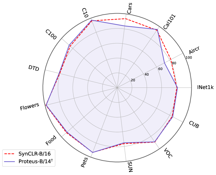
Figure 4: Comparison on ImageNet linear evaluation and fine-grained classification with SynCLR. ^†Proteus is distilled from SynCLR-L/14.

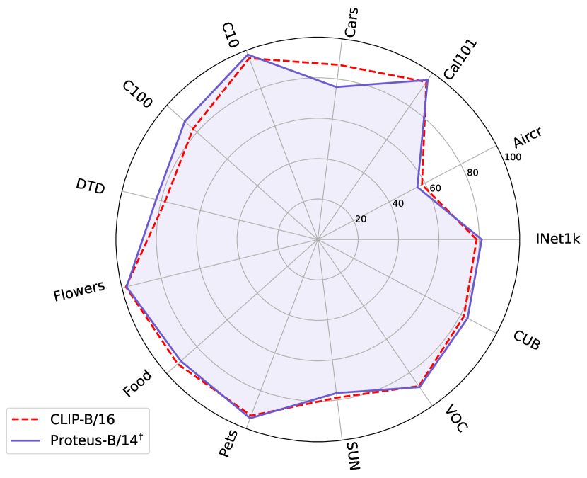
Figure 5: Comparison on ImageNet linear evaluation and fine-grained classification with CLIP. ^†Proteus is distilled from CLIP-L/14.

4 Analysis

4.1 Proxy Task

In this section, we conduct analyses on the proxy task to verify the effectiveness of our design. We first examine the effectiveness of removing the designs that lead to dataset bias. Then, we conduct ablation to validate our proposed three different levels of learning objectives.

Combating Dataset Bias. To study the importance of mitigating dataset bias, we start with the conventional knowledge distillation setting of ViT [59], which leverages hard logits distillation and combines the Cross-Entropy loss with the KL-divergence loss [31]. Note that we do not introduce the extra distillation token like DeiT and keep the same structure as the teacher model. Shown in Tab. 4.1, the default distillation setting of DeiT delivers very good ImageNet accuracy. However, its generalization ability (fine-grained classification) remains at the same level as distillation from ImageNet pre-trained teacher (78.7$\%$ versus 77.8$\%$), indicating that it does not fully utilize the fruitful knowledge of the foundation teacher model. We then empirically change hard logits to soft logits and remove the CE loss as the one-hot label will introduce the dataset bias. The results support our hypothesis as soft logits distillation without CE loss delivers the highest accuracy on fine-grained classification among the four choices. Further, we revise the design to distilling before the FC layer as it implicitly introduces the dataset bias, which brings significant improvement to generalizability.

Table 8: Ablation study on combating dataset bias. ViT-S/14 models are distilled from DINOv2-B on ImageNet-1K for 300 epochs.

Source	KL	CE	MSE	ImageNet	Fine-grained
Hard Logits	✔	✔		82.8	78.7
Soft Logits	✔	✔		80.3	71.5
Hard Logits	✔			81.7	79.7
Soft Logits	✔			82.3	80.5
Hint			✔	81.7	85.3

Table 9: Ablation study on learning objectives. ViT-S/14 models are distilled from DINOv2-B on ImageNet-1K for 300 epochs.

Token	Feature	Patch	ImageNet	Fine-grained	ADE20K
✔			81.7	85.3	44.0
	✔		79.2	83.3	47.0
✔	✔		81.7	86.1	47.4
✔	✔	✔	81.8	85.8	50.0

Learning Objective. Although hint distillation already achieves very good results on classification tasks, it is not enough to fully transfer the knowledge of foundation models as the results on semantic segmentation are not good (44.0$\%$ versus 51.0$\%$). The explanation is that classification tasks only utilize the classification token which has been distilled from the teacher, whereas semantic segmentation requires the whole feature for dense prediction. Shown in Tab. 4.1, the performance is boosted both on classification and dense prediction after adding the feature-level learning objective. Considering that DINOv2 [43] is trained with patch-level learning objective [74], we mimic this behavior to enforce the student to predict the tokenized representation of the masked patch and it delivers very good performance across various tasks.

Table 10: Comparison on ImageNet linear evaluation and fine-grained classification with different proxy datasets. We follow the default protocol of Proteus to train ViT-S/14 distilled by DINOv2-B/14.

Dataset	ImageNet	Aircraft	Cal101	Cars	C10	C100	DTD	Flowers	Food	Pets	SUN	VOC	CUB	Average
ImageNet-1K	81.8	65.5	95.1	77.0	97.8	87.3	78.4	99.0	87.9	95.7	71.7	87.1	86.7	85.8
ImageNet-Merge	81.8	68.5	95.3	79.9	98.1	87.1	79.6	99.0	91.1	95.5	72.9	87.5	86.4	86.7
ImageNet-Single	63.7	51.2	86.4	46.9	88.4	72.7	71.9	92.3	67.0	64.4	61.0	78.3	43.4	68.7

4.2 Proxy Dataset

While we have already demonstrated that ImageNet-1K serves as a good proxy dataset because we successfully compress foundation models on it, we further study the importance of the proxy dataset by introducing multiple variants: (1) ImageNet-Merge: Following the idea of DINOv2 [43] and SynCLR [54], we simply concatenate all the training sets that we utilized for validation, including ImageNet-1K, 12 fine-grained datasets, ADE20K and NYU-Depth V2. It results in a training set of 1.4M images. (2) ImageNet-Single: We build a 1.2M training set where the images are generated from a single large image by performing extensive data augmentations [4, 3]. (3) ImageNet-sub-data: we randomly sample a portion of data at each class with the ratio of 20$\%$ and 50$\%$. (4) ImageNet-sub-class: we randomly sample a portion of classes from the total 1000 classes with the ratio of 20$\%$ and 50$\%$. Please refer to Sec. A.11 for more details.

Dataset Diversity. We first conduct ablation on ImageNet-Merge and ImageNet-Single to study the property of dataset diversity. Shown in Tab. 10, ImageNet-Merge brings almost 1$\%$ average improvement on fine-grained classification with merely 0.2M additional data, which suggests the importance of a diverse dataset. We further consider the extreme case where all the source information comes from a single image and it surprisingly delivers very decent performance. Specifically, 6 out of 12 datasets suffer from performance drop over 10$\%$ while the remaining ones exhibit acceptable results considering that most of the classes in those fine-grained datasets are missing in this single image. This demonstrates that Proteus is robust even under the extreme scenario.

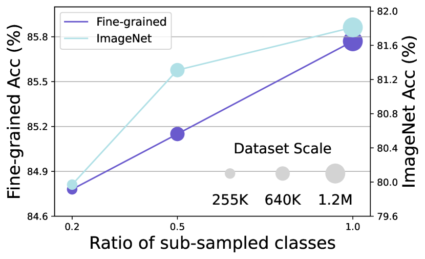
Figure 6: Comparisons on ImageNet linear evaluation and fine-grained classification on ImageNet-1K with sub-sampled classes.

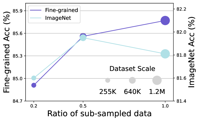
Figure 7: Comparisons on ImageNet linear evaluation and fine-grained classification on ImageNet-1K with sub-sampled data per class.

Scaling Behavior. All ViT-S/14 models are distilled from DINOv2-B/14 for 375K iterations with a batch size of 1024. Fig. 7 shows that there is a minor performance drop (1$\%$) at fine-grained accuracy even when we only sample 200 classes out of 1000. More surprisingly, the ImageNet linear probing accuracy only decreases by 1.8$\%$ when we sample 200 classes (80$\%$ of the classes are not seen by the model during pre-training). Fig. 7 suggests a similar phenomenon but there are two differences: (1) sub-sampling data suffers from less performance drop which indicates that data diversity is more important than the number of data per class. (2) There is a 0.1$\%$ increase in ImageNet accuracy when sampling 50$\%$ of the data, which we hypothesize is due to the variance in linear probing. To summarize, these two figures demonstrate the robustness of Proteus when subjected to reduced data availability, suggesting that it is feasible to access foundation models with even smaller data scales.

5 Related Work

Supervised Learning approaches [22, 51, 30] used to dominate the research community of computer vision. These methods provide valuable experience in model architecture design, which benefit the research in different domains [71, 72] and lay a solid foundation for the introduction of the transformer architecture [60, 14]. Nevertheless, the reliance on extensively annotated datasets [13, 34, 17] inherent in supervised learning models presents significant limitations. Additionally, supervised learning can struggle with generalization outside of the training dataset [27, 48], especially in cases where the distribution of the training data does not accurately reflect real-world scenarios.

Self-supervised Learning has emerged as a powerful paradigm for leveraging unlabeled data, significantly reducing the dependency on extensive labeled datasets. Contrastive learning methods [10, 21, 42, 56, 18] foster invariance to different transformations of the same image while segregating the representations of distinct images [63]. On the other hand, masked image modeling [7, 20, 64, 74, 6] involves either pixel reconstruction [20] or local feature regeneration [6], often yielding impressive results when fine-tuning for dense prediction tasks [20]. In the landscape of vision foundation models, strategies such as DINOv2 [43] and CLIP [46] have set new benchmarks for versatility and robustness. However, both approaches conduct large-scale training on private gigantic datasets, presenting substantial challenges for training foundation models in a similar vein.

Model Compression

techniques like Knowledge Distillation [26, 44, 2, 55, 59] and Pruning [19, 32, 40, 36] have been extensively studied for task-specific model compression. Howeverm task-agnostic model compression, which maintains the generalization ability, has become rather important in the era of foundation models [46, 43, 54]. Nevertheless, there remain two critical challenges: (1) The training data of those foundation models is rarely disclosed [46, 43, 54]. (2) Training those foundation models requires significantly large training resources and it is a common protocol to utilize the original dataset to perform task-agnostic model compression [65, 43]. To address these issues, we consider the setting of data-free model compression with limited data.

6 Discussion

Limitation. Due to computational constraints, we only validate our model on ImageNet-1K, and its efficacy at a larger scale dataset remains unverified. Besides, Proteus has to keep the same patch size as the teacher model because of the introduced patch and feature-level learning objectives.

Broader Impact. Discussed in Sec. 3.2.3, Proteus comprehensively surpasses the supervised learning method across all metrics, demonstrating its potential to serve as a training paradigm for those supervised learning approaches. Besides, our work supports the research in model compression so that foundation models can be compressed at a much smaller cost. Further, we have shown in Sec. 4.2 that it is possible to access foundation models at even smaller datasets compared to ImageNet-1K, which may be a promising avenue for future exploration. Moreover, while our work mainly focuses on the pure vision foundation models with image modality, we hope our work can incentivize the exploration of this idea in Large Language Models (LLMs) and Large Multimodal Models (LMMs) to facilitate the research under the era of foundation models.

Conclusion. In this paper, we propose Proteus, a simple and general distillation framework to transfer the general-purpose visual representations from foundation models into the target network with ‘limited’ data (ImageNet-1K). Specifically, we remove the designs from conventional knowledge distillation that could lead to dataset bias and present three levels of training objectives, i.e., token, patch, and features, to promise the application across various tasks. We conduct extensive experiments to verify the scalability and generalization ability of Proteus and provide comprehensive analysis.

Appendix A Appendix

A.1 Implementation Details

A.1.1 Pre-training

We strictly follow the DeiT [59] training protocol on ImageNet-1K [13] except that we do not enable Mixup [70]. All models are training for 300 epochs with a batch size of 1024 on 8 A100 GPUs, except the ViT-L experiment with a batch size of 256 due to GPU memory constraints. We adopt the masking strategy in iBOT [74] for the patch-level learning objective.

A.1.2 ImageNet Linear Probing

For all ImageNet linear probing results, we follow the linear probing protocol outlined in DINOv2 [43]. Specifically, the linear layer is trained using the SGD optimizer for 25,020 iterations with a batch size of 512. We employ random-resized-crop data augmentation and conduct a grid search over the hyperparameters as defined in DINOv2. We report the best accuracy on the validation set in accordance with prior works.

A.1.3 Fine-grained linear classification

Following SynCLR [54], we train a regularized multinomial logistic regression model on the output classification token. During training and testing, no data augmentation is applied; images will be resized to 224 along the shorter side, followed by a center crop of 224×224. The training objective is minimized using L-BFGS with L2-regularization and the L2-regularization constant is chosen on the validation set from 45 logarithmically spaced values between $10^{-6}$ and $10^{3}$. Unlike DINOv2 [43] and SynCLR, We reduce the maximum number of L-BFGS iterations from 1000 to 500 for faster evaluation.

A.1.4 Semantic Segmentation

We conduct experiments on ADE20K dataset [73] using the single-scale setup. We adopt the resolution of 512$\times$512 for models that are trained with the patch size of 16$\times$16 and 518$\times$518 for patch size of 14$\times$14. Linear: we follow the setup and hyperparameters in iBOT [74] and use FCN [37] as the linear layer to perform probing on the frozen backbone. Fine-tune: we adhere to the setup and hyperparameters in SynCLR [54] which utilizes UperNet [68] as the task adaptation layer.

A.1.5 Depth Estimation

We evaluate the methods on the NYU-Depth V2 [50] dataset. Similar with semantic segmentation, we utilize a resolution of 512$\times$512 for models trained with a patch size of 16$\times$16, and a resolution of 518$\times$518 for models trained with a patch size of 14$\times$14. We always adopt DPT [47] as the decoder under both evaluation protocols. Fine-tune: we follow to the setup and hyperparameters in the public codebase [33]. Linear: we utilize the same hyperparameters in the Fine-tune protocol except that we enlarge the learning rate from 1e-4 to 4e-4.

A.2 Weight Inheritance

Table 11: Ablation study of Weight Inheritance on DeiT where the model is trained with the standard protocol on ImageNet-1K for 300 epochs.

Arch	Inherit	Teacher	ImageNet
DeiT-Ti	N/A	N/A	71.9
DeiT-Ti	DeiT-S	N/A	73.5
DeiT-Ti	N/A	DeiT-S	73.7
DeiT-Ti	DeiT-S	DeiT-S	74.8

Table 12: Ablation study of Weight Inheritance on DINOv2 where the model is trained with the standard protocol on ImageNet-1K for 300 epochs.

Arch	Inherit	Teacher	ImageNet
DINOv2-Ti	N/A	N/A	75.4
DINOv2-Ti	DINOv2-S	N/A	75.8
DINOv2-Ti	N/A	DINOv2-S	77.5
DINOv2-Ti	DINOv2-S	DINOv2-S	77.2

Existing methods to compress foundation models often utilize the pre-trained weights either by structure pruning [38, 66] or weight inheritance [65, 69]. However, structure pruning requires complex setups and is not general enough to be adapted to arbitrary architectures. Weight Selection [69] proves that initializing smaller models with uniformly selected weights from a pre-trained larger model results in better performance. Besides, TinyCLIP [65] shows simply inheriting the weights from the teacher network, i.e., the foundation model, with a fixed pattern can improve the distillation efficiency. Following the design of Weight Selection, we conduct ablation on DeiT [59] and DINOv2 [43], where the pre-trained weights are learned with supervised learning objective and self-supervised learning objective, respectively. Table A.2 demonstrates that weight inheritance is advantageous for DeiT training, whether knowledge distillation is applied or not. Conversely, as shown in Table A.2, weight inheritance is less effective for DINOv2 and can even be detrimental when knowledge distillation is used. We conjecture that this phenomenon is caused by the mismatch between the downstream learning objective (supervised learning) and the pre-training learning objective (self-supervised learning), while both the teacher and student of DeiT are trained with the supervised learning objective.

To validate this point, we conduct ablation on weight inheritance and Tab. 13 shows that directly inheriting the pre-trained weights results in performance degradation at all classification benchmarks. Therefore, we simply leverage the randomly initialized network as the student to maintain the generalization ability of Proteus, so that it could be applied to different foundation models which are learned with various learning objectives.

Table 13: Comparison on ImageNet linear evaluation and fine-grained classification with ablation on weight inheritance. We follow the default protocol of Proteus to train ViT-S/14 with DINOv2-B/14.

Method	Inherit	ImageNet	Aircraft	Cal101	Cars	C10	C100	DTD	Flowers	Food	Pets	SUN	VOC	CUB	Average
Proteus	✔	81.5	64.5	94.9	75.9	97.7	86.6	78.2	98.8	87.7	94.9	71.1	87.0	86.4	85.3
Proteus		81.8	65.5	95.1	77.0	97.8	87.3	78.4	99.0	87.9	95.7	71.7	87.1	86.7	85.8

A.3 Robustness Evaluation

We compare Proteus with DINOv2 on ImageNet variants for robustness evaluation. We utilize the models that are obtained by linear probing on ImageNet-1K and run inference on those datasets. Shown in Tab. 14, Proteus achieves similar results with DINOv2 on ImageNet-Sketch, ImageNet-R and outperforms it obviously on ImageNet-C. However, we fall behind DINOv2 at ImageNet-A at different scales which may be caused by the lack of training data.

Table 14: Comparison with DINOv2 on robustness evaluation.

Method	Dataset	Arch	Teacher	Accuracy	Robustness
				Im-Val	Im-S	Im-A	Im-R	Im-C$\downarrow$
DINOv2	LVD-142M	ViT-S/14	DINOv2-g/14	81.2	40.2	34.1	53.4	54.3
Proteus	ImageNet-1.2M	ViT-S/14	DINOv2-B/14	81.8	39.8	31.1	51.0	50.5
DINOv2	LVD-142M	ViT-B/14	DINOv2-g/14	83.4	50.5	55.5	63.9	42.8
Proteus	ImageNet-1.2M	ViT-B/14	DINOv2-L/14	84.9	51.0	52.4	63.4	38.6
DINOv2	LVD-142M	ViT-L/14	DINOv2-g/14	86.3	59.4	71.4	74.6	31.4
Proteus	ImageNet-1.2M	ViT-L/14	DINOv2-g/14	86.2	59.8	68.7	73.9	29.9

A.4 More Diverse Proxy Dataset for CLIP

While we have shown that Proteus achieves similar average accuracy on fine-grained classification with CLIP [46] when leveraging CLIP-L/14 as the teacher, it is worth noting that the performance at certain datasets, e.g., StanfordCars and FGVC-Aircraft, is obviously worse than CLIP. We conjecture the limitation is caused by the diversity of ImageNet-1K so we reconduct the experiments with ImageNet-Merge. Shown in Tab.15, the accuracy of these datasets increases significantly, even outperforming CLIP on FGVC-Aircraft. This indicates that the performance of Proteus can be easily enhanced by a more diverse dataset.

Table 15: Comparison on fine-grained classification with more diverse proxy dataset. We distill CLIP-L/14 to ViT-B/14.

Method	Dataset	Aircraft	Cal101	Cars	C10	C100	DTD	Flowers	Food	Pets	SUN	VOC	CUB	Average
CLIP-B/16	WIT-400M	58.3	94.7	87.0	95.9	82.6	78.0	97.9	92.8	93.2	78.8	88.2	81.8	85.8
Proteus-B/14	ImageNet-1K	55.7	95.9	76.0	97.8	88.1	82.5	97.6	90.7	94.5	76.5	88.7	83.8	85.7
Proteus-B/14	ImageNet-Merge	62.8	96.4	86.8	97.9	88.6	81.8	98.4	94.1	94.2	78.8	88.8	84.9	87.8

A.5 Dense Prediction for SynCLR

In the main text, we have compared Proteus with SynCLR [54] on the classification tasks when utilizing it as the teacher network. As SynCLR is also trained with the patch-level objective iBOT [74], it exhibits strong performance on dense prediction tasks. We further fine-tune the pre-trained backbones on semantic segmentation dataset ADE20K [73] and utilize UperNet [68] as the task adaptation layer. Shown in Tab. 16, Proteus lags behind SynCLR only by 0.9$\%$ which is acceptable considering the small scale dataset that we use. It further demonstrates the generalization ability of Proteus as SynCLR is trained with a very different learning objective on the large synthetic dataset.

Table 16: Comparison on semantic segmentation dataset ADE20K with SynCLR. ^†Proteus is distilled from SynCLR ViT-L/14.

Method	Arch	text	img	# imgs	mIoU
SynCLR	ViT-B/16	synthetic	synthetic	600M	53.4
Proteus†	ViT-B/14	N/A	real	1.2M	52.5

A.6 Generalization to out-of-domain Concepts

Following SynCLR [54], we evaluate the pre-trained models on two additionally fine-grained datasets: GTSRB [52] and Country211 [46]. These two datasets are not in the retrival list or concept list in DINOv2 and SynCLR, therefore considered as out-of-domain concepts. Tab. 17 shows that DINOv2 and SynCLR obtain obviously worse performance compared to CLIP, possibly because its training data included similar concepts. While Proteus achieves very similar results with its counterparts on both datasets by mimicking the teacher’s pattern, indicating its strong generalization ability across different foundation models.

Table 17: Generalization to concepts not seen by DINOv2 and SynCLR.

Method	Arch	Teacher	GTSRB	Country211
DINOv2	ViT-B/14	DINOv2-g/14	73.5	21.8
Proteus	ViT-B/14	DINOv2-L/14	76.4	19.4
SynCLR	ViT-B/16	N/A	78.5	21.0
Proteus	ViT-B/14	SynCLR-L/14	81.5	21.4
CLIP	ViT-B/16	N/A	88.2	32.3
Proteus	ViT-B/14	CLIP-L/14	87.6	29.3

A.7 Teacher Choice

In the default setting of Proteus, we choose the pre-trained model at a larger scale to serve as our teacher network and we conduct ablation with teacher at different scales for analysis. Shown in Tab. 18, the average accuracy of Proteus decreases with the increased teacher scales. This may seem counterintuitive as a larger teacher contains more fruitful knowledge and has stronger ability. However, there exists a dimension gap between teacher and student, and a projection head is utilized to align the dimensions between them. Assumably, a larger teacher denotes a lager gap between the dimension and information may be lost during the projection. This facilitates the application of Proteus because smaller teachers will speedup the training process significantly compared with giant teacher models.

Table 18: Comparison on fine-grained classification with different teacher choices. We follow the default protocol of Proteus to train ViT-S/14 with different teachers. ^† denotes the official DINOv2-S model which is distilled from DINOv2-g.

Teacher	Aircraft	Cal101	Cars	C10	C100	DTD	Flowers	Food	Pets	SUN	VOC	CUB	Average
DINOv2-g/14†	74.4	96.5	80.8	97.7	87.7	80.3	99.5	89.2	95.1	74.5	88.0	87.5	87.6
DINOv2-g/14	60.3	89.4	69.8	96.7	83.0	70.9	94.1	82.7	94.9	63.0	85.2	77.3	80.6
DINOv2-L/14	58.0	93.3	67.7	97.4	84.7	74.1	96.3	84.0	95.4	67.6	86.9	80.9	82.2
DINOv2-B/14	65.5	95.1	77.0	97.8	87.3	78.4	99.0	87.9	95.7	71.7	87.1	86.7	85.8

A.8 Training Efficiency

We compare with the supervised learning method DeiT [59] in terms of training efficiency as both methods are trained on ImageNet-1K for 300 epochs. We measure the time on the same platform, i.e., 8 A100 GPUs. Shown in Tab. 19, Proteus consumes similar training hours with DeiT as our training objectives are very easy. Moreover, we find the validation after each training epoch actually costs lots of time in DeiT. In contrast, we perform pre-training on ImageNet-1K and only conduct linear probing after the training, which can be finished within one hour.

Table 19: Ablation study on projector design. ViT-S/14 models are distilled from DINOv2-B on ImageNet-1K for 300 epochs.

Method	Arch	Teacher	Training Hour	Validation Hour
DeiT	ViT-S/16	RegNetY	30	9
Proteus	ViT-S/14	DINOv2-B/14	30	1

A.9 Projection Head Design

Here we conduct ablation on the design of the projection head which is used to align the dimension between teacher and student model. Tab. 20 shows that different combination results in similar performance but Layer Normalization (LN) [5] leads to slightly better accuracy in terms of the two metrics. We adopt this design in all our experiments without fine-tuning for better strategy.

Table 20: Ablation study on projector design. ViT-S/14 models are distilled from DINOv2-B on ImageNet-1K for 300 epochs.

Design	ImageNet	Fine-grained
Linear+GELU	81.8	84.9
GELU+Linear	81.5	85.3
LN+Linear	81.7	85.3

A.10 Visualization Implementations

Following the procedure in DINOv2 [43] and SynCLR [54], we perform PCA on the image patches from the same set and colorize them using their first three components. We resize the images to 518$\times$518 to fit the patch size of 14 and the pictures are captured from the Internet.

A.11 Composition of Proxy Dataset

Shown in Tab. 21 and Fig. 8, we provide detailed information about the proxy datasets that we used in Sec. 4.2.

Table 21: Proxy Dataset composition.

Dataset	# imgs	Source
ImageNet-Merge	1.4M	ImageNet-1K, ADE20K, NYUd, 12 fine-grained datasets
ImageNet-Single	1.2M	Single Image (see Fig. 8)
ImageNet-sub-data (50$\%$)	640K	ImageNet-1K
ImageNet-sub-class (50$\%$)	640K	ImageNet-1K
ImageNet-sub-data (20$\%$)	255K	ImageNet-1K
ImageNet-sub-class (20$\%$)	255K	ImageNet-1K

Figure 8: Picture that is used to generate ImageNet-Single.

A.12 List of Benchmarks for Evaluation

We show the list of benchmarks used for evaluation in Tab. 22.

Table 22: List of benchmarks used for evaluation.

Dataset name	Task	Citation
ImageNet-1K	Image Classification	[13]
ImageNet-A	Image Classification	[25]
ImageNet-C	Image Classification	[24]
ImageNet-Rendition	Image Classification	[23]
ImageNet-Sketch	Image Classification	[62]
Food-101	Image Classification	[8]
CIFAR-10	Image Classification	[29]
CIFAR-100	Image Classification	[29]
SUN397	Image Classification	[67]
StanfordCars	Image Classification	[28]
FGVC-Aircraft	Image Classification	[39]
Pascal VOC 2007	Image Classification	[15]
Describable Textures	Image Classification	[12]
Oxford Pets	Image Classification	[45]
Caltech101	Image Classification	[16]
Oxford Flowers	Image Classification	[41]
CUB200	Image Classification	[61]
GTSRB	Image Classification	[52]
Country211	Image Classification	[46]
ADE20K	Image Segmentation	[73]
NYU-Depth V2	Monocular Depth Estimation	[50]

References

- [1] R. Adriana, B. Nicolas, K. S. Ebrahimi, C. Antoine, G. Carlo, and B. Yoshua. Fitnets: Hints for thin deep nets. ICLR, 2015.
- [2] S. Ahn, S. X. Hu, A. Damianou, N. D. Lawrence, and Z. Dai. Variational information distillation for knowledge transfer. In CVPR, 2019.
- [3] Y. M. Asano, C. Rupprecht, and A. Vedaldi. A critical analysis of self-supervision, or what we can learn from a single image. arXiv preprint arXiv:1904.13132, 2019.
- [4] Y. M. Asano and A. Saeed. The augmented image prior: Distilling 1000 classes by extrapolating from a single image. arXiv preprint arXiv:2112.00725, 2021.
- [5] J. L. Ba, J. R. Kiros, and G. E. Hinton. Layer normalization. arXiv preprint arXiv:1607.06450, 2016.
- [6] A. Baevski, W.-N. Hsu, Q. Xu, A. Babu, J. Gu, and M. Auli. Data2vec: A general framework for self-supervised learning in speech, vision and language. In ICML, 2022.
- [7] H. Bao, L. Dong, S. Piao, and F. Wei. Beit: Bert pre-training of image transformers. arXiv preprint arXiv:2106.08254, 2021.
- [8] L. Bossard, M. Guillaumin, and L. Van Gool. Food-101–mining discriminative components with random forests. In ECCV, 2014.
- [9] M. Caron, H. Touvron, I. Misra, H. Jégou, J. Mairal, P. Bojanowski, and A. Joulin. Emerging properties in self-supervised vision transformers. In ICCV, 2021.
- [10] T. Chen, S. Kornblith, M. Norouzi, and G. Hinton. A simple framework for contrastive learning of visual representations. In ICML, 2020.
- [11] M. Cherti, R. Beaumont, R. Wightman, M. Wortsman, G. Ilharco, C. Gordon, C. Schuhmann, L. Schmidt, and J. Jitsev. Reproducible scaling laws for contrastive language-image learning. In CVPR, 2023.
- [12] M. Cimpoi, S. Maji, I. Kokkinos, S. Mohamed, and A. Vedaldi. Describing textures in the wild. In CVPR, 2014.
- [13] J. Deng, W. Dong, R. Socher, L.-J. Li, K. Li, and L. Fei-Fei. Imagenet: A large-scale hierarchical image database. In CVPR, 2009.
- [14] A. Dosovitskiy, L. Beyer, A. Kolesnikov, D. Weissenborn, X. Zhai, T. Unterthiner, M. Dehghani, M. Minderer, G. Heigold, S. Gelly, et al. An image is worth 16x16 words: Transformers for image recognition at scale. arXiv preprint arXiv:2010.11929, 2020.
- [15] M. Everingham, S. A. Eslami, L. Van Gool, C. K. Williams, J. Winn, and A. Zisserman. The pascal visual object classes challenge: A retrospective. IJCV, 2015.
- [16] L. Fei-Fei, R. Fergus, and P. Perona. Learning generative visual models from few training examples: An incremental bayesian approach tested on 101 object categories. In CVPRW, 2004.
- [17] A. Geiger, P. Lenz, and R. Urtasun. Are we ready for autonomous driving? the kitti vision benchmark suite. In CVPR, 2012.
- [18] R. Hadsell, S. Chopra, and Y. LeCun. Dimensionality reduction by learning an invariant mapping. In CVPR, 2006.
- [19] S. Han, H. Mao, and W. J. Dally. Deep compression: Compressing deep neural networks with pruning, trained quantization and huffman coding. arXiv preprint arXiv:1510.00149, 2015.
- [20] K. He, X. Chen, S. Xie, Y. Li, P. Dollár, and R. Girshick. Masked autoencoders are scalable vision learners. In CVPR, 2022.
- [21] K. He, H. Fan, Y. Wu, S. Xie, and R. Girshick. Momentum contrast for unsupervised visual representation learning. In CVPR, 2020.
- [22] K. He, X. Zhang, S. Ren, and J. Sun. Deep residual learning for image recognition. In CVPR, 2016.
- [23] D. Hendrycks, S. Basart, N. Mu, S. Kadavath, F. Wang, E. Dorundo, R. Desai, T. Zhu, S. Parajuli, M. Guo, et al. The many faces of robustness: A critical analysis of out-of-distribution generalization. In ICCV, 2021.
- [24] D. Hendrycks and T. Dietterich. Benchmarking neural network robustness to common corruptions and perturbations. arXiv preprint arXiv:1903.12261, 2019.
- [25] D. Hendrycks, K. Zhao, S. Basart, J. Steinhardt, and D. Song. Natural adversarial examples. In CVPR, 2021.
- [26] G. Hinton, O. Vinyals, J. Dean, et al. Distilling the knowledge in a neural network. arXiv preprint arXiv:1503.02531, 2015.
- [27] P. W. Koh, S. Sagawa, H. Marklund, S. M. Xie, M. Zhang, A. Balsubramani, W. Hu, M. Yasunaga, R. L. Phillips, I. Gao, et al. Wilds: A benchmark of in-the-wild distribution shifts. In ICML, 2021.
- [28] J. Krause, M. Stark, J. Deng, and L. Fei-Fei. 3d object representations for fine-grained categorization. In ICCVW, 2013.
- [29] A. Krizhevsky, G. Hinton, et al. Learning multiple layers of features from tiny images. 2009.
- [30] A. Krizhevsky, I. Sutskever, and G. E. Hinton. Imagenet classification with deep convolutional neural networks. NeurIPS, 2012.
- [31] S. Kullback. Information theory and statistics. Courier Corporation, 1997.
- [32] H. Li, A. Kadav, I. Durdanovic, H. Samet, and H. P. Graf. Pruning filters for efficient convnets. arXiv preprint arXiv:1608.08710, 2016.
- [33] Z. Li. Monocular depth estimation toolbox. https://github.com/zhyever/Monocular-Depth-Estimation-Toolbox, 2022.
- [34] T.-Y. Lin, M. Maire, S. Belongie, J. Hays, P. Perona, D. Ramanan, P. Dollár, and C. L. Zitnick. Microsoft coco: Common objects in context. In ECCV, 2014.
- [35] Z. Liu and K. He. A decade’s battle on dataset bias: Are we there yet? arXiv preprint arXiv:2403.08632, 2024.
- [36] Z. Liu, M. Sun, T. Zhou, G. Huang, and T. Darrell. Rethinking the value of network pruning. arXiv preprint arXiv:1810.05270, 2018.
- [37] J. Long, E. Shelhamer, and T. Darrell. Fully convolutional networks for semantic segmentation. In CVPR, 2015.
- [38] X. Ma, G. Fang, and X. Wang. Llm-pruner: On the structural pruning of large language models. NeurIPS, 2023.
- [39] S. Maji, E. Rahtu, J. Kannala, M. Blaschko, and A. Vedaldi. Fine-grained visual classification of aircraft. arXiv preprint arXiv:1306.5151, 2013.
- [40] P. Molchanov, S. Tyree, T. Karras, T. Aila, and J. Kautz. Pruning convolutional neural networks for resource efficient inference. arXiv preprint arXiv:1611.06440, 2016.
- [41] M.-E. Nilsback and A. Zisserman. Automated flower classification over a large number of classes. In 2008 Sixth Indian conference on computer vision, graphics & image processing. IEEE, 2008.
- [42] A. v. d. Oord, Y. Li, and O. Vinyals. Representation learning with contrastive predictive coding. arXiv preprint arXiv:1807.03748, 2018.
- [43] M. Oquab, T. Darcet, T. Moutakanni, H. Vo, M. Szafraniec, V. Khalidov, P. Fernandez, D. Haziza, F. Massa, A. El-Nouby, et al. Dinov2: Learning robust visual features without supervision. arXiv preprint arXiv:2304.07193, 2023.
- [44] W. Park, D. Kim, Y. Lu, and M. Cho. Relational knowledge distillation. In CVPR, 2019.
- [45] O. M. Parkhi, A. Vedaldi, A. Zisserman, and C. Jawahar. Cats and dogs. In CVPR, 2012.
- [46] A. Radford, J. W. Kim, C. Hallacy, A. Ramesh, G. Goh, S. Agarwal, G. Sastry, A. Askell, P. Mishkin, J. Clark, et al. Learning transferable visual models from natural language supervision. In ICML, 2021.
- [47] R. Ranftl, A. Bochkovskiy, and V. Koltun. Vision transformers for dense prediction. In ICCV, 2021.
- [48] B. Recht, R. Roelofs, L. Schmidt, and V. Shankar. Do imagenet classifiers generalize to imagenet? In ICML, 2019.
- [49] C. Schuhmann, R. Vencu, R. Beaumont, R. Kaczmarczyk, C. Mullis, A. Katta, T. Coombes, J. Jitsev, and A. Komatsuzaki. Laion-400m: Open dataset of clip-filtered 400 million image-text pairs. arXiv preprint arXiv:2111.02114, 2021.
- [50] N. Silberman, D. Hoiem, P. Kohli, and R. Fergus. Indoor segmentation and support inference from rgbd images. In ECCV, 2012.
- [51] K. Simonyan and A. Zisserman. Very deep convolutional networks for large-scale image recognition. arXiv preprint arXiv:1409.1556, 2014.
- [52] J. Stallkamp, M. Schlipsing, J. Salmen, and C. Igel. The german traffic sign recognition benchmark: a multi-class classification competition. In IJCNN, 2011.
- [53] R. Taori, I. Gulrajani, T. Zhang, Y. Dubois, X. Li, C. Guestrin, P. Liang, and T. B. Hashimoto. Stanford alpaca: An instruction-following llama model, 2023.
- [54] Y. Tian, L. Fan, K. Chen, D. Katabi, D. Krishnan, and P. Isola. Learning vision from models rivals learning vision from data. arXiv preprint arXiv:2312.17742, 2023.
- [55] Y. Tian, D. Krishnan, and P. Isola. Contrastive representation distillation. arXiv preprint arXiv:1910.10699, 2019.
- [56] Y. Tian, D. Krishnan, and P. Isola. Contrastive multiview coding. In ECCV, 2020.
- [57] T. Tommasi, N. Patricia, B. Caputo, and T. Tuytelaars. A deeper look at dataset bias. Domain adaptation in computer vision applications, pages 37–55, 2017.
- [58] A. Torralba and A. A. Efros. Unbiased look at dataset bias. In CVPR, 2011.
- [59] H. Touvron, M. Cord, M. Douze, F. Massa, A. Sablayrolles, and H. Jégou. Training data-efficient image transformers & distillation through attention. In ICML, 2021.
- [60] A. Vaswani, N. Shazeer, N. Parmar, J. Uszkoreit, L. Jones, A. N. Gomez, Ł. Kaiser, and I. Polosukhin. Attention is all you need. NeurIPS, 2017.
- [61] C. Wah, S. Branson, P. Welinder, P. Perona, and S. Belongie. The caltech-ucsd birds-200-2011 dataset. 2011.
- [62] H. Wang, S. Ge, Z. Lipton, and E. P. Xing. Learning robust global representations by penalizing local predictive power. NeurIPS, 2019.
- [63] T. Wang and P. Isola. Understanding contrastive representation learning through alignment and uniformity on the hypersphere. In ICML, 2020.
- [64] C. Wei, H. Fan, S. Xie, C.-Y. Wu, A. Yuille, and C. Feichtenhofer. Masked feature prediction for self-supervised visual pre-training. In CVPR, 2022.
- [65] K. Wu, H. Peng, Z. Zhou, B. Xiao, M. Liu, L. Yuan, H. Xuan, M. Valenzuela, X. S. Chen, X. Wang, et al. Tinyclip: Clip distillation via affinity mimicking and weight inheritance. In ICCV, 2023.
- [66] M. Xia, T. Gao, Z. Zeng, and D. Chen. Sheared llama: Accelerating language model pre-training via structured pruning. arXiv preprint arXiv:2310.06694, 2023.
- [67] J. Xiao, J. Hays, K. A. Ehinger, A. Oliva, and A. Torralba. Sun database: Large-scale scene recognition from abbey to zoo. In CVPR, 2010.
- [68] T. Xiao, Y. Liu, B. Zhou, Y. Jiang, and J. Sun. Unified perceptual parsing for scene understanding. In ECCV, 2018.
- [69] Z. Xu, Y. Chen, K. Vishniakov, Y. Yin, Z. Shen, T. Darrell, L. Liu, and Z. Liu. Initializing models with larger ones. arXiv preprint arXiv:2311.18823, 2023.
- [70] H. Zhang, M. Cisse, Y. N. Dauphin, and D. Lopez-Paz. mixup: Beyond empirical risk minimization. arXiv preprint arXiv:1710.09412, 2017.
- [71] Y. Zhang, K. Li, K. Li, L. Wang, B. Zhong, and Y. Fu. Image super-resolution using very deep residual channel attention networks. In ECCV, 2018.
- [72] Y. Zhang, Y. Tian, Y. Kong, B. Zhong, and Y. Fu. Residual dense network for image super-resolution. In CVPR, 2018.
- [73] B. Zhou, H. Zhao, X. Puig, S. Fidler, A. Barriuso, and A. Torralba. Scene parsing through ade20k dataset. In CVPR, 2017.
- [74] J. Zhou, C. Wei, H. Wang, W. Shen, C. Xie, A. Yuille, and T. Kong. ibot: Image bert pre-training with online tokenizer. arXiv preprint arXiv:2111.07832, 2021.