Quantum weak values and the “which way?” question

Abstract

Uncertainty principle forbids one to determine which of the two paths a quantum system has travelled, unless interference between the alternatives had been destroyed by a measuring device, e.g., by a pointer. One can try to weaken the coupling between the device and the system, in order to avoid the veto. We demonstrate, however, that a weak pointer is at the same time an inaccurate one, and the information about the path taken by the system in each individual trial is inevitably lost. We show also that a similar problem occurs if a classical system is monitored by an inaccurate quantum meter. In both cases one can still determine some characteristic of the corresponding statistical ensemble, a relation between path probabilities in the classical case, and a relation between the probability amplitudes if a quantum system is involved.

I Introduction

There is a well known difficulty with determining the path taken by a quantum system capable of reaching a known final state via several alternative routes. According to the Uncertainty Principle FeynL such determination is possible only if an additional measuring device destroys interference between the alternatives. However, the device inevitably perturbs the system’s motion, and alters the likelihood of its arrival at the desired final state. The knowledge of the system’s past must, therefore, be incompatible with maintaining the probability of a successful post-selection intact.

A suitable measuring device can be a pointer vN , designed to move only if the system travels the chosen path, so that finding it displaced at the end of experiment could constitute a proof of the system’s past. A somewhat naive way around the Uncertainty Principle may be the use a pointer coupled to the system only weakly, thus leaving interference between the paths almost intact. Perhaps the small change of the pointer’s final state could provide “which path?” (“which way?”) information previously deemed to be unavailable?

The idea is not new, and was applied, for example, to an optical realisation of a three-path problem 3P1 -3P2 . The conclusion of that the photons can be found in a part of the setup they can neither enter nor leave, and must therefore have discontinuous trajectories, was subsequently criticised by a number of authors 3Pc1 -3Pc3 for both technical and more fundamental reasons. A similar treatment of a four-path “quantum Cheshire cat” 4P1 -4P3 model suggests a possibility of separating a system from its property, to wit, electrons detached from their charges, and an atom’s internal energy “disembodied” from the atom itself. (For further discussion of the model the reader is referred to 4P4 ). The case for a quantum particle (or, at least, of some of its “properties”) being in several interfering pathways at the same time was recently made in Matz .

Here our more modest aim is to analyse, in some detail, the validity of the approach in the case of the simplest “double slit” (two-path) problem.

The rest of the paper is organised as follows. Section II briefly describes the well known quantum double-slit experiment. A classical analogue of the problem is studied in Sections III-VI. A simple two-way quantum problem is analysed in Sects. VII-XI. Section XII contains our conclusions.

II Quantum “which way?” problem

One of the unanswered questions in quantum theory, indeed its “only mystery” FeynC , concerns the behaviour of a quantum particle in a double-slit experiment shown in Fig.1. The orthodox FeynL view is as follows. With only two observable events, preparation and final detection, it is impossible to claim that the particle has gone via one of the slits (paths) and not the other. This is because the rate of detection by the detector in Fig.1 may increase if one of the paths is blocked FeynL .

Neither is it possible to claim that both paths were travelled at the same time, since an additional inspection never finds only fraction of a photon in one of the paths FeynC .

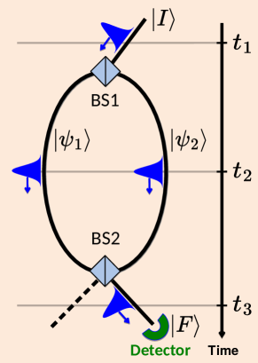
Figure 1: An optical realisation of a “double-slit” experiment. At time $t_{1}$, a photon’s wave packet $|I\rangle$ is split into two at the first beam splitter (BS1). Its parts, $|\psi_{1}\rangle$ and $|\psi_{2}\rangle$, travel both optic fibres, $t_{2}$, and are recombined into $|F\rangle$ after the second BS2, $t_{3}$. The two observed events are initial preparation, and final detection of the photon. Where was the photon between these two events?

However, such an inspection destroys the interference between the paths, and alters the probability of detection. The problem is summarised in the Uncertainty Principle FeynC : “It is impossible to design any apparatus whatsoever to determine through which hole the particle passes that will not at the same time disturb the particle enough to destroy the interference.”

The approach of 3P1 may suggest a way around this verdict. If two von Neumann pointers vN , set up to measure projectors on the paths (e.g., on the states $|\psi_{1}\rangle$ and $|\psi_{2}\rangle$ in Fig.1) are coupled to the particle only weakly, interference between the paths can be preserved. If, in addition, both pointers are found to “have moved”, albeit on average, the “weak traces” 3P1 left by the particle will reveal its presence in both paths at the same time. The idea appears to contradict the Uncertainty Principle and, for this reason, deserves our attention. We start the investigation by looking first at inaccurate pointers designed to monitor a classical stochastic system in Fig.2.

III Consecutive measurements of a classical system

Our simple classical model is as follows. (We ask for reader’s patience. The quantum case will be discussed shortly). A system (one can think of a little ball rolling down a network of connected tubes shown in Fig.2) is introduced into one of the two inputs at $t=t_{1}$, with a probability $w_{i}$, $i=0,1$. It then passes through states $j$ and $k$, where $j,k=0,1$ at the times $t_{2}$, and $t_{3}$, respectively. The experiment is finished when the system is collected in a state $l$, $l=0,1$ at $t=t_{4}$. From each state $i$, the system is directed to one of the states $j$ with a probability $p(j\leftarrow i)$, similarly from $j$ to $k$, and finally from $k$ to $l$. There are altogether eight paths $\{l\leftarrow k\leftarrow j\leftarrow i\}$, each travelled with a probability

$$P(l\leftarrow k\leftarrow j\leftarrow i)=p(l\leftarrow k)p(k\leftarrow j)p(j\leftarrow i),$$ (1)

$$p(k\leftarrow j)=\delta_{jk},$$

where $\delta_{jk}$ is the Kroneker delta. (The choice of this design will become clear shortly.)

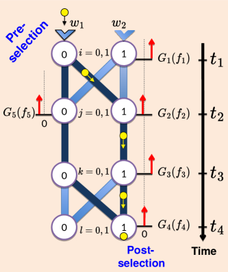
Figure 2: A classical two-state system can reach a final state by taking one of the the eight paths with a probability given by Eq.(1). The system can be monitored with the help of pointers (red arrows), which move if the system is detected [cf. Eq.(2)]. Also shown (in dark blue) is the two-way problem of Sect. IV.

We make the following assumptions.

1. Alice, the experimenter, knows the paths probabilities in Eq.(1), but not the input values $w_{i}$.

2. She cannot observe the system directly, and relies on the readings of pointers with positions $f_{n}$, $n=1,2...5$, installed at different locations, as shown in Fig.2. If the system passes through a location, the corresponding pointer is displaced by a unit length, $f_{n}\to f_{n}+1$, otherwise it is left intact.

3. The pointers are, in general, inaccurate, since their initial positions are distributed around zero with probabilities $G_{n}(f_{n})$ (see Fig.2). Their final positions are, however, determined precisely. We will consider the distributions $G_{n}$ to be Gaussians of widths $\Delta f_{n}$,

   $$G_{n}(f_{n})=\sqrt{\frac{1}{\pi\Delta f_{n}^{2}}}\exp\left(-\frac{f_{n}^{2}}{\Delta f_{n}^{2}}\right),$$ (2)

   $$\int G_{n}(f_{n})df_{n}=1,\quad G_{n}(f_{n}){\xrightarrow[\Delta f_{n}\to 0]{}}\delta(f_{n}).$$

The experiment ends just after $t=t_{4}$, when Alice’s observed outcomes are the five numbers $f_{n}$, $n=1,\dots,5$. These are distributed with a probability density

$$\rho(f_{1},f_{2},f_{3},f_{4},f_{5})=\sum_{i,j,k,l=0,1}w_{i}P(l\leftarrow k\leftarrow j\leftarrow i)G_{1}(f_{1}-i)G_{2}(f_{2}-j)G_{3}(f_{3}-k)G_{4}(f_{4}-l)G_{5}(f_{5}+j-1).$$ (3)

Equation (3) is not particularly useful, since $w_{i}$ are unknown. However, by making the first pointer accurate, $\Delta f_{1}\to 0$, $G_{1}(f_{1})\to\delta(f_{1}-i)$ where $\delta(x)$ is the Dirac delta, she is able to pre-select those cases where, say, $f_{1}=0$, and collect only the corresponding statistics. Now the (properly normalised) distribution of the remaining four readings does not depend on $w_{i}$,

$$\rho_{0}(f_{2},f_{3},f_{4},f_{5})=\sum_{j,k,l=0,1}P(l\leftarrow k\leftarrow j\leftarrow 0)\times\quad$$ (4)

$$G_{2}(f_{2}-j)G_{3}(f_{3}-k)G_{4}(f_{4}-l)G_{5}(f_{5}+j-1),$$

and Alice has a complete description of the pre-selected ensemble.

Alice can also post-select the system by selecting, e.g., the cases where it ends in a state $1$ at $t=t_{4}$. With $G_{4}(f_{4})\to\delta(f_{4}-1)$, the remaining random variables $f_{2}$, $f_{3}$, and $f_{5}$ are distributed according to [cf. Fig.2 and Eq.(1)]

$$\rho_{1\leftarrow 0}(f_{2},f_{3},f_{5})=\quad\quad\quad\quad\quad\quad\quad\quad\quad\quad\quad\quad$$ (5)

$$\frac{\sum_{j=0,1}P_{j}G_{2}(f_{2}-j)G_{3}(f_{3}-j)G_{5}(f_{5}+j-1)}{P_{0}+P_{1}},$$

where we introduced a shorthand

$$P_{j}\equiv P(1\leftarrow j\leftarrow j\leftarrow 0),\quad j=0,1.$$ (6)

Equation (4) suggests a simple, yet useful, general criterion.

• Alice can determine the system’s past location only when she obtains a pointer’s reading whose likelihood depends only on the probabilities of the system’s paths passing through that location.

For example, at least three accurate readings ($f_{1}$, $f_{4}$ and one of $f_{2}$,$f_{3}$, or $f_{5}$,) are needed if Alice is to know which of the eight paths shown in Fig.2 the system has travelled during each trial. With $G_{n}(f_{n})=\delta(f_{n})$ for $n=1,2,4$, a trial can yield. e.g., values $f_{1}=0$, $f_{2}=1$, and $f_{4}=1$. The likelihood of these outcomes is given by the probability $P(1\leftarrow 1\leftarrow 1\leftarrow 0)$ in Eq.(1), and Alice can be certain that the route $\{1\leftarrow 1\leftarrow 1\leftarrow 0\}$ has indeed been travelled.

IV A classical “two-way problem”

Consider next a pre- and post-selected ensemble with two routes connecting the states $0$ at $t=t_{1}$ and $1$ at $t=t_{4}$ (shown in Fig.2 in dark blue). As a function of the second pointer’s accuracy, $\Delta f_{2}$, the distribution of its readings (5) changes from a bimodal, when the pointer is accurate,

$$\rho_{1\leftarrow 0}(f_{2}) \equiv\int\rho_{1\leftarrow 0}(f_{2},f_{3},f_{5})df_{3}df_{5}$$

$$=\frac{P_{0}G_{2}(f_{2})+P_{1}G_{2}(f_{2}-1)}{P_{0}+P_{1}}$$

$${\xrightarrow[\Delta f_{2}\to 0]{}}\frac{P_{0}\delta(f_{2})+P_{1}\delta(f_{2}-1)}{P_{0}+P_{1}}$$ (7)

to the original broad Gaussian for an inaccurate pointer,

$$\rho_{1\leftarrow 0}(f_{2}){\xrightarrow[\Delta f_{2}\to\infty]{}}\thinspace\thinspace G_{2}(f_{2}-z),\quad\quad\quad$$ (8)

displaced as a whole by

$$z=\frac{P_{1}}{P_{0}+P_{1}}.$$ (9)

Equation (8) reflects a known property of Gaussians, to our knowledge first explored in Vaid , and discussed in detail in Appendix A. The transformation of two peaks (IV) into a single maximum (8) is best described by the catastrophe theory Cata . For example, for $P_{0}=P_{1}$, a pitchfork bifurcation converts two maxima and a minimum into a single maximum for $\Delta f_{2}=\sqrt{2}$ (see Appendix B).

With a sufficiently accurate pointer, $\Delta f_{2}\ll 1$, a reading always lies close to $0$ or $1$, and in every trial Alice knows the path followed by the system.

With a highly inaccurate pointer, $\Delta f_{2}\gg 1$, not a single reading $f_{2}$ can be attributed to one path in preference to the other, and the route by which the system arrived at its final state is never known (see Appendix C). Indeed, for $P_{0}=P_{1}$, even the most probable outcome, $f_{2}=1/2$ is equally likely to occur if the system takes path $\{1\leftarrow 0\leftarrow 0\leftarrow 0\}$, or $\{1\leftarrow 1\leftarrow 1\leftarrow 0\}$,

$$\rho\left(f_{2}=\frac{1}{2}\right)={\frac{1}{2}}\left[G_{2}\left(\frac{1}{2}\right)+G_{2}\left(-\frac{1}{2}\right)\right],$$ (10)

and the “which way?” information is clearly lost.

Still, something can be learnt about a pre- and post-selected classical ensemble, even without knowing the path taken by the system. Having performed many trials, Alice can evaluate an average reading,

$$\langle f_{2}\rangle\equiv\int f_{2}\rho_{1\leftarrow 0}(f_{2})df_{2}=z.\quad\quad\quad$$ (11)

The quantity $z$ in Eqs.(9) and (11) is the relative (i.e., renormalised to a unit sum) probability of travelling the path $\{1\leftarrow 1\leftarrow 1\leftarrow 0\}$, and is independent of $\Delta f_{2}$. Thus, by using an inaccurate pointer, Alice can still estimate certain parameters of her statistical ensemble.

V Two inaccurate classical pointers and a wrong conclusion

A word of caution should be added against an attempt to recover the “which way?” information with the help of Eq.(11). For two equally inaccurate pointers, $\Delta f_{2}=\Delta f_{5}\equiv\Delta f\gg 1$, [cf. Fig.2] the distribution of the readings tends to a single Gaussian shown in Fig.3a (see also Appendix A),

$$\rho_{1\leftarrow 0}(f_{2},f_{5})=\quad\quad\quad\quad\quad\quad\quad\quad\quad\quad\quad\quad$$ (12)

$$\frac{P_{0}G_{2}(f_{2})G_{5}(f_{5}-1)+P_{1}G_{2}(f_{2}-1)G_{5}(f_{5})}{P_{0}+P_{1}}\quad\quad\quad$$

$${\xrightarrow[\Delta f\to\infty]{}}\thinspace G_{2}(f_{2}-z_{2})G_{5}(f_{5}-z_{5}),\quad\quad\quad\quad\quad$$

where

$$z_{2}=\frac{P_{1}}{P_{0}+P_{1}},\quad z_{5}=\frac{P_{0}}{P_{0}+P_{1}}=1-z_{2}.$$ (13)

It may seem that (the reader can already see where we are going with this),

1. Each pointer in Eq.(12) “moves” only when the system is in its path.

2. Eq.(12) suggests that both pointers have moved (albeit on average).

3. Hence, the system must be travelling both paths at the same time.

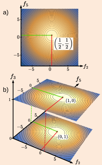
Figure 3: a) Distribution of the readings $\rho_{1\leftarrow 0}(f_{2},f_{5})$ of two inaccurate pointers with $P_{0}=P_{1}$ and $\Delta f_{2}=\Delta f_{5}=10$, monitoring a classical system at $t=t_{2}$ [cf. Eq.(12)]; b) The distribution $\rho_{1\leftarrow 0}(f_{2},f_{3},f_{5})$ in Eq.(14) with an accurate pointer, $\Delta f_{3}\to 0$, added at $t=t_{3}$. Note that integration of the distribution in (b) over $df_{3}$ recovers the distribution shown in (a).

To check if this is the case, Alice can add an accurate pointer ($f_{3}$) acting at $t=t_{3}$ (see Fig.2). If parts of the system were in both places at $t_{2}$, the same must be true at $t_{3}$, since Alice made sure that no pathway connects the points $j=0$ and $k=1$. The accurate pointer should, therefore, always find only a part of the system. Needless to say, this is not what happens. With an additional accurate pointer in place, three dimensional distribution (5) becomes bimodal, again (see Fig.3b)

$$\rho_{1\leftarrow 0}(f_{2},f_{3},f_{5})=(P_{0}+P_{1})^{-1}\times$$ (14)

$$\big{[}P_{0}G_{2}(f_{2})G_{5}(f_{5}-1)\delta(f_{3})+$$

$$P_{1}G_{2}(f_{2}-1)G_{5}(f_{5})\delta(f_{3}-1)\big{]}$$ .

An inspection of statistics collected separately for $f_{3}=0$ or $f_{3}=1$ shows that at $t=t_{2}$ only one of the two pointers moves in any given trial. Contour plots of the densities in Eqs.(12) and (14) are shown in Figs.3a and b, respectively. The fallacy (i)-(iii), evident in our classical example, will become less obvious in the quantum case we will study after a brief digression.

VI Classical “hidden variables”

Before considering the quantum case, it may be instructive to add a fourth assumption to the list of Sect.III.

1. In Alice’s world all pointers have the property that an accurate detection inevitably perturbs the system’s evolution.

For example, whenever the pointer $f_{3}$ moves, the probabilities $p(l\leftarrow 1)$ in Eq.(1) are reset to $p^{\prime}(l\leftarrow 1,\Delta f_{3})$. Thus, $P_{1}$ changes to $P^{\prime}_{1}(\Delta f_{3}$), while $P_{0}$ remains the same. The change may be the greater the smaller is $\Delta f_{3}$, and $P^{\prime}_{1}(\Delta f_{3}\to\infty)=P_{1}$. Now the system, accurately observed in the state $1$ at $t_{3}$ arrives in state $1$ at $t=t_{4}$, say, less frequently than it would with no pointer ($f_{3}$) in place, $P_{0}+P^{\prime}_{1}(\Delta f_{3}\to 0)<P_{0}+P_{1}$. So, where was the unobserved system at $t=t_{3}$?

Empirically, the question has no answer. To ensure the arrival rate is unchanged by observation, Alice can only use an inaccurate pointer, $\Delta f_{3}\ \gg 1$, which yields no “which way?” information. Performing many trials, she can, however, measure both the probability of arriving in $1$ at $t=t_{4}$, $W_{1}(t_{4})=P_{0}+P^{\prime}_{1}(\Delta f_{3}\gg 1)\approx P_{0}+P_{1}$ and the value of $z=P^{\prime}_{1}(\Delta f_{3}\gg 1)/[P_{0}+P^{\prime}_{1}(\Delta f_{3}\gg 1)]\approx P_{1}/[P_{0}+P_{1}]$ [cf. Eqs.(8) and (9)]. She can then evaluate unperturbed path probabilities,

$$P_{1}\approx zW_{1}(t_{4}),\quad P_{0}\approx(1-z)W_{1}(t_{4}).$$ (15)

Having observed that $P_{0}$ and $P_{1}$ are both positive, and do not exceed unity, Alice may reason about what happens to unobserved system in the following manner. Available empirical data is consistent with the system always following one of the two paths with probabilities in Eq.(15). However, with the available instruments, it is not possible to verify this conclusion experimentally.

This is as close as we can get to the quantum case using a classical toy model. We consider the quantum case next.

VII Consecutive measurements of a qubit

A quantum analogue of the classical model just discussed is shown in Fig.4. Experiment, in which Alice monitors the evolution of a two-level quantum system (qubit) with a Hamiltonian $\hat{H}^{s}$ by means of five von Neumann pointers, begins at $t=t_{1}$ and ends at $t=t_{4}$. With no transitions between the states $|b_{0(1)}\rangle$ and $|c_{1(0)}\rangle$ there are altogether eight virtual (Feynman) paths which connect the initial and final states. Just before $t_{1}$ the qubit may be thought to be in some state $|\Psi_{\text{in}}\rangle$, and the eight path amplitudes are given by ($i,j,k,l=0,1$)[cf. Fig.4]

$$\mathcal{A}^{s} (F_{l}\leftarrow c_{j}\leftarrow b_{j}\leftarrow I_{i})=$$ (16)

$$a (F_{l}\leftarrow c_{j})a(c_{j}\leftarrow b_{j})a(b_{j}\leftarrow I_{i}),$$

where $a(b_{j}\leftarrow I_{i})=\langle b_{j}|\hat{U}^{s}(t_{2}-t_{1})|I_{i}\rangle$ etc., and $\hat{U}^{s}(t)\equiv\exp(-i\hat{H}^{s}t)$ is the qubit’s own evolution operator.

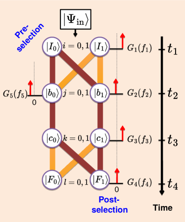
Figure 4: A two-level quantum system can reach final states $|F_{l}\rangle$, $l=0,1$, via eight virtual paths whose probability amplitudes are given by Eq.(16). The system is monitored by means of von Neumann pointers (red arrows), set to measure projectors $\hat{\pi}_{n}$ [cf. Eq.(17)]. Also shown (in maroon) is the “double-slit problem” of Sect.VIII.

We note the following.

1. Alice the experimenter knows the path amplitudes in Eq.(16), but not the system’s input state $|\Psi_{\text{in}}\rangle$. (If she did, the experiment would begin earlier, at the time $|\Psi_{\text{in}}\rangle$ was first determined.)

2. Alice cannot look at the system directly, and has access only to von Neumann pointers vN with positions $f_{n}$, and momenta $\lambda_{n}$, $n=1,...5$, (see Fig.4). The pointers are briefly coupled to the system at $t=t_{n}$, ($t_{5}\equiv t_{2}$), via

   $$\hat{H}^{\text{int}}_{n} =-i\partial_{f_{n}}\hat{\pi}_{n}\delta(t-t_{n}),\quad\hat{\pi}_{n}=|X_{n}\rangle\langle X_{n}|,$$ (17)

   $$|X_{n}\rangle =|I_{1}\rangle,|b_{1}\rangle,|c_{1}\rangle,|F_{1}\rangle,|b_{0}\rangle,\quad n=1,...5.$$

   and have no own dynamics.

3. The pointers, initially in states $|G_{n}\rangle$, are inaccurate, with initial positions distributed around zero with probability amplitudes $G_{n}(f_{n})\equiv\langle f_{n}|G_{n}\rangle$. We will consider Gaussian pointers,

   $$G_{n}(f_{n}) =\left(\frac{2}{\pi\Delta f_{n}^{2}}\right)^{1/4}\exp\left(-\frac{f_{n}^{2}}{\Delta f_{n}^{2}}\right),$$ (18)

   $$\int G^{2}_{n}(f_{n})df_{n} =1,\quad\quad G^{2}_{n}(f_{n}){\xrightarrow[\Delta f_{n}\to 0]{}}\delta(f_{n}).$$

4. A pointer perturbs the qubit’s evolution, except in the limit $\Delta f_{n}\to\infty$. Indeed, replacing $f_{n}$ with $f_{n}^{\prime}=f_{n}/\Delta f_{n}$ changes $\hat{H}^{\text{int}}$ in Eq.(17) to $\hat{H}^{\text{int}^{\prime}}=\hat{H}^{\text{int}}/\Delta f_{n}$, and a highly inaccurate pointer decouples from the qubit 4P4 . Vice versa, a weakly coupled pointer is, necessarily, an inaccurate one.

As in the classical case, to be able to make statistical predictions, Alice needs to make the first measurement accurate, $\Delta f_{1}\to 0$, $G^{2}_{1}(f_{1})\to\delta(f_{1})$, and pre-select, e.g., only those cases where $f_{1}=0$, preparing thereby the system in the state $|I_{0}\rangle$. The rest of the readings are distributed according to (we use $\tilde{\rho}$ to distinguish from the classical distributions of Sects. III-V)

$$\tilde{\rho}_{0}(f_{2},f_{3},f_{4},f_{5})=\sum_{l=0,1}|G_{4}(f_{4}-l)|^{2} \times$$ (19)

$$\bigg{|}\sum_{j=0,1}G_{3}(f_{3}-j)G_{2}(f_{2}-j) \times$$

$$G_{5}(f_{5}+j-1)\mathcal{A}^{s}{(F_{l}\leftarrow c_{j}\leftarrow b_{j}\leftarrow I_{0})} \bigg{|}^{2}.$$

As in the classical case, Alice can also post-select the qubit, e.g., in a state $|F_{1}\rangle$, by choosing $\Delta f_{4}\to 0$, $G^{2}_{4}(f_{4})\to\delta(f_{4})$, and collecting the statistics only if $f_{1}=0$ and $f_{4}=1$. The distribution of the remaining three readings is given by

$$\tilde{\rho}_{1\leftarrow 0}(f_{2},f_{3},f_{5})=W_{1}(t_{4})^{-1}\times\quad\quad\quad$$ (20)

$$\bigg{|}\sum_{j=0,1}G_{3}(f_{3}-j)G_{2}(f_{2}-j)G_{5}(f_{5}+j-1)\mathcal{A}^{s}_{j}\bigg{|}^{2},$$

where we introduced a shorthand

$$\mathcal{A}^{s}_{j}\equiv\mathcal{A}^{s}(F_{1}\leftarrow c_{j}\leftarrow b_{j}\leftarrow I_{0}),\quad j=0,1.$$ (21)

The normalisation factor $W_{1}(t_{4})\equiv\int\rho_{1\leftarrow 0}(f_{2},f_{3},f_{5})$ $df_{2}df_{3}df_{5}$ is the probability of reaching the final state $|F_{1}\rangle$ with all three pointers in place, which depends on the pointers’ accuracies,

$$W_{1}(t_{4}) =|\mathcal{A}^{s}_{0}|^{2}+|\mathcal{A}^{s}_{1}|^{2}+2J_{2}J_{3}J_{5}\text{Re}\left[{\mathcal{A}^{s}_{0}}^{*}\mathcal{A}^{s}_{1}\right],$$ (22)

$$J_{n} \equiv\int G_{n}(f_{n})G_{n}(f_{n}-1)df_{n}=\exp\left(\frac{-1}{2\Delta f_{n}^{2}}\right).$$

The general rule of the previous Section can be extended to the quantum case as follows.

• Alice may ascertain the qubit’s condition, represented by a state in its Hilbert space, only when she obtains a pointer’s reading whose probability depends only on the system’s path amplitudes for the paths passing through the state in question.

As in the classical case, three accurate measurements allow one to determine the path followed by the qubit. For example, with $\Delta f_{1},\Delta f_{2},\Delta f_{4}\to 0$, outcomes $f_{1}=0$, $f_{2}=1$, $f_{4}=1$, whose probability is

$$P(1,1,0)\equiv\int_{-\epsilon}^{\epsilon}df_{2}\int_{1-\epsilon}^{1+\epsilon}df_{4}\int_{-\infty}^{\infty}df_{3}df_{5}$$ (23)

$$\times\tilde{\rho}_{0}(f_{2},f_{3},f_{4},f_{5}){\xrightarrow[\Delta f_{2},\thinspace\Delta f_{4}\to 0]{}}|\mathcal{A}^{s}_{1}|^{2}$$ ,

indicates that qubit has followed the path $\{F_{1}\leftarrow c_{1}\leftarrow b_{1}\leftarrow I_{0}\}$ (see Fig.4).

VIII A quantum “double-slit” problem

The simple model shown in Fig.4 has the essential features of the setup shown in Fig.1, and is simple to analyse. Two paths connect the initial and final states, $|I_{0}\rangle$ at $t=t_{1}$ and $|F_{1}\rangle$ at $t=t_{4}$; pointers $f_{2}$ and $f_{5}$ monitor the presence of the qubit in each path at $t=t_{2}$, and the pointer $f_{3}$ can be used for additional control. For simplicity, Alice can decouple two pointers from the qubit by sending

$$\Delta f_{3},\Delta f_{5}\to\infty,\quad J_{3},J_{5}\to 1.$$ (24)

As a function of the remaining pointer’s accuracy, $\Delta f_{2}$, the distribution of its readings (20) changes from bimodal,

$$\tilde{\rho}_{1\leftarrow 0}(f_{2})\equiv\int\tilde{\rho}_{1\leftarrow 0}(f_{2},f_{3},f_{5})df_{3}df_{5}\quad\quad$$ (25)

$${\xrightarrow[\Delta f_{2}\to 0]{}}\frac{|\mathcal{A}^{s}_{0}|^{2}\delta(f_{2})+|\mathcal{A}^{s}_{1}|^{2}\delta(f_{2}-1)}{|\mathcal{A}^{s}_{0}|^{2}+|\mathcal{A}^{s}_{1}|^{2}},$$

to a single broad Gaussian,

$$\tilde{\rho}_{1\leftarrow 0}(f_{2})=\frac{|G_{2}(f_{2})\mathcal{A}^{s}_{0}+G_{2}(f_{2}-1)\mathcal{A}^{s}_{1}|^{2}}{|\mathcal{A}^{s}_{0}|^{2}+|\mathcal{A}^{s}_{1}|^{2}+2\text{Re}\left[{\mathcal{A}^{s}}^{*}_{0}\mathcal{A}^{s}_{1}\right]}$$ (26)

$${\xrightarrow[\Delta f_{2}\to\infty]{}}\quad G^{2}_{2}(f_{2}-\tilde{z}),\quad\quad\quad$$

displaced as a whole by

$$\tilde{z}=\text{Re}\left[\frac{\mathcal{A}^{s}_{1}}{\mathcal{A}^{s}_{0}+\mathcal{A}^{s}_{1}}\right],$$ (27)

where we have used Eq.(49) of Appendix D. The transformation between the two forms is similar to transformation of the classical probability from (IV) to (8) (see Appendix D).

As in the classical case, with an accurate pointer, $\Delta f_{2}\ll 1$, a reading is always either $0$ or $1$, and in every trial Alice knows the path followed by the qubit.

For a highly inaccurate pointer, $\Delta f_{2}\gg 1$, there is not a single reading $f_{2}$ which can be attributed to one path in preference to the other (cf. Appendix C), so Alice never knows how the qubit arrived at its final state. Indeed, even the probability of the most likely reading, $f_{2}=\tilde{z}$, contains contributions from each path,

$$\tilde{\rho}_{1\leftarrow 0}(f_{2}=\tilde{z})=\frac{|\mathcal{A}^{s}_{0}G_{2}(\tilde{z})+\mathcal{A}^{s}_{1}G_{2}(\tilde{z}-1)|^{2}}{|\mathcal{A}^{s}_{0}+\mathcal{A}^{s}_{1}|^{2}}.$$ (28)

However, Alice may gain information about a pre- and post-selected ensemble even without knowing the path chosen by the qubit. Having performed many trials (it will take more trials the larger is $\Delta f_{2}$), she can evaluate the average reading, i.e. first moment,

$$\langle f_{2}\rangle_{1\leftarrow 0}\equiv\int f_{2}\tilde{\rho}_{1\leftarrow 0}(f_{2})df_{2}=\quad\quad\quad$$ (29)

$$\frac{|\mathcal{A}^{s}_{1}|^{2}+J_{2}\text{Re}[{\mathcal{A}^{s}_{0}}^{*}\mathcal{A}^{s}_{1}]}{|\mathcal{A}^{s}_{0}|^{2}+|\mathcal{A}^{s}_{1}|^{2}+2J_{2}\text{Re}[{\mathcal{A}^{s}_{0}}^{*}\mathcal{A}^{s}_{1}]}{\xrightarrow[\Delta f_{2}\to\infty]{}}\tilde{z}.$$

There is no contradiction with the Uncertainty Principle, which permits knowing the amplitudes $\mathcal{A}^{s}_{i}$, [and, therefore, their particular combination (27)]. What the Principle forbids is using this knowledge to answer, among other things, the “which way?” question. We illustrate this by the next example.

IX Two inaccurate quantum pointers, and another conclusion not to make

As in the classical case, Alice can employ at $t=t_{2}$ two highly inaccurate pointers, $\Delta f_{2}=\Delta f_{5}\equiv\Delta f\gg 1$, which measure projectors on the states $|b_{0}\rangle$ and $|b_{1}\rangle$, respectively. Now, by Eq.(52), the distribution of the readings is Gaussian,

$$\tilde{\rho}_{1\leftarrow 0}(f_{2},f_{5})=\quad\quad\quad\quad\quad\quad\quad\quad\quad\quad$$ (30)

$$\frac{|\mathcal{A}^{s}_{0}G_{2}(f_{2})G_{5}(f_{5}-1)+\mathcal{A}^{s}_{1}G_{2}(f_{2}-1)G_{5}(f_{5})|^{2}}{|\mathcal{A}^{s}_{0}|^{2}+|\mathcal{A}^{s}_{1}|^{2}+2J_{2}J_{5}\text{Re}\left[{\mathcal{A}^{s}}^{*}_{0}\mathcal{A}^{s}_{1}\right]}$$

$${\xrightarrow[\Delta f\to\infty]{}}G_{2}^{2}(f_{2}-\tilde{z}_{2})G_{5}^{2}(f_{5}-\tilde{z}_{5}),\quad\quad$$

where

$$\tilde{z}_{2}=\text{Re}\left[\frac{\mathcal{A}^{s}_{1}}{\mathcal{A}^{s}_{0}+\mathcal{A}^{s}_{1}}\right],\quad\tilde{z}_{5}=\text{Re}\left[\frac{\mathcal{A}^{s}_{0}}{\mathcal{A}^{s}_{0}+\mathcal{A}^{s}_{1}}\right]=1-\tilde{z}_{2}.$$ (31)

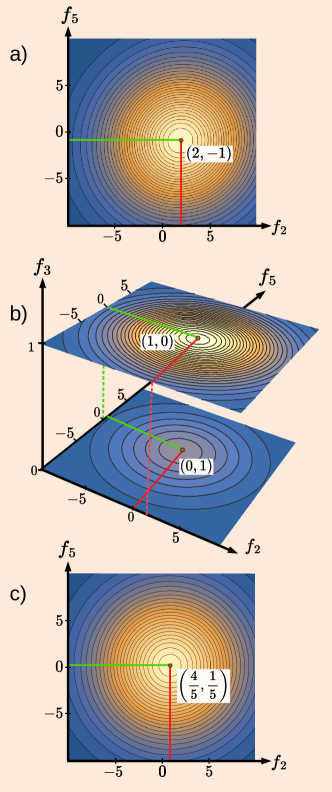
Figure 5: a) Distribution of the readings $\tilde{\rho}_{1\leftarrow 0}(f_{2},f_{5})$ of two inaccurate quantum pointers with $\mathcal{A}^{s}_{0}=-\mathcal{A}^{s}_{1}/2$ and $\Delta f_{2}=\Delta f_{5}=10$, monitoring a qubit at $t=t_{2}$ [cf. Eq.(30)]; b) The distribution $\tilde{\rho}_{1\leftarrow 0}(f_{2},f_{3},f_{5})$ in Eq.(32) with an accurate pointer, $\Delta f_{3}=0$, added at $t=t_{3}$. c) The result of integrating the distribution in (b) over $df_{3}$. Note that in (c) one does not recover the distribution shown in (a).

And, as in the classical case, we encourage the reader to avoid the following reasoning (see section VIII).

1. A pointer “moves” (“weak trace” 3P1 is produced) [cf. Eq.(26)] only when the qubit is in the state upon which the projection is made.

2. Eq.(30) suggests that both pointers have moved (albeit on average).

3. Hence, there is experimental evidence of the qubit’s presence in both states at $t=t_{2}$ and, therefore, in both paths connecting $|I_{0}\rangle$ with $|F_{1}\rangle$.

As in the classical case, we find the fault with using the position of the maximum of the distribution (30). As was shown in the previous Section, an inaccurate quantum pointer looses the “which way?” information. The information cannot, therefore, be recovered by employing two, or more, such pointers to predict the presence of the qubit in a given state.

In FeynC it was pointed out that assuming that in a double slit experiment the particle passes through both slits at the same time may lead to a wrong prediction. Namely, only a part of an electron, or photon, would need to be detected at the exit of a slit, and this is not what happens in practice. Next we briefly review the argument of FeynC in the present context.

X A “wrong prediction”

If not convinced by the argument of the previous Section, Alice can follow the advice of FeynC , and attempt to study qubit’s evolution in more detail. In particular, she can add an accurate pointer acting at $t=t_{3}$ (see Fig.4), in order to detect only a part of the qubit travelling along the path $\{F_{1}\leftarrow c_{1}\leftarrow b_{1}\leftarrow I_{0}\}$. If the distribution (30) is a proof of the qubit being present in both paths at $t_{2}$ in any meaningful sense, this must be the only logical expectation. Since there is no path connecting $|b_{0}\rangle$ with $|c_{1}\rangle$ (see Fig.4), two parts of the qubit cannot recombine in $|c_{1}\rangle$ at $t_{3}>t_{2}$.

However, at $t=t_{3}$ Alice finds either a complete qubit, or no qubit at all. As, $\Delta f_{3}\to 0$, the distribution (20) becomes bimodal in a three dimensional space ($f_{2}$,$f_{3}$,$f_{5}$)

$$\tilde{\rho}_{1\leftarrow 0}(f_{2},f_{3},f_{5}){\xrightarrow[\Delta f_{3}\to 0]{}}\frac{|\mathcal{A}^{s}_{0}|^{2}G^{2}_{2}(f_{2})\delta(f_{3})G^{2}_{5}(f_{5}-1)}{|\mathcal{A}^{s}_{0}|^{2}+|\mathcal{A}^{s}_{1}|^{2}}$$ (32)

$$+\frac{|\mathcal{A}^{s}_{1}|^{2}G^{2}_{2}(f_{2}-1)\delta(f_{3}-1)G^{2}_{5}(f_{5})}{|\mathcal{A}^{s}_{0}|^{2}+|\mathcal{A}^{s}_{1}|^{2}}$$ .

Possible values of $f_{3}$ are $0$ and $1$, and only one of the pointers acting at $t=t_{2}$ is seen to “move” in any given trial. Contour plots of the densities in Eqs.(30) and (32) are shown in Figs.5a and b, respectively. Note that integrating the density in Fig.5b over $df_{3}$ does not reproduce that in Figs.5a, but rather the density (12)[cf. Fig.3a] for a classical system with $P_{0}=1/5$ and $P_{1}=4/5$, shown in Figs.5c.

One can still argue that Alice does not compare like with like, since the added accurate pointer perturbs qubit’s evolution in a way that makes it choose the path $\{F_{1}\leftarrow c_{1}\leftarrow b_{1}\leftarrow I_{0}\}$. The difficulty with this explanation is well known in the analysis of delayed choice experiments DL1 . Decision to couple the accurate pointer may be taken by Alice after $t_{2}$, and cannot be expected to affect the manner in which the qubit passes through the states $|b_{0}\rangle$ and $|b_{1}\rangle$. This argument usually serves as a warning against naive realistic picture for interpreting quantum phenomena DL1 . Conclusion in the case studied here is even simpler. “Weak traces” are not faithful indicators of the system’s presence at a given location, and using them as such leads to avoidable contradictions.

XI Quantum “hidden variables”

In order to keep the rate of successful post-selections intact, $W_{1}(t_{4})=|\mathcal{A}^{s}_{0}+\mathcal{A}^{s}_{1}|^{2}$, Alice may only use weakly coupled and, therefore, inaccurate pointers. These, as was shown above, yield no information as to whether the qubit was in the state $|b_{0}\rangle$ or $|b_{1}\rangle$ at $t=t_{2}$ in any given trial, so the question remains unanswerable in principle. The same is true for classical inaccurate pointers in Sect. VI, but there it was possible to deduce the probabilities, $P_{0}$ and $P_{1}$, with which the system travels each of the two paths [cf. Eq.(15)]. In quantum case, an attempt to find directly unobservable “hidden” path probabilities governing statistical behaviour of an unobserved system fails for a simple reason. With no a priori restrictions on the signs of $\mathcal{A}^{s}_{i}$, the measured $\tilde{z}$ in Eq.(27) can have any real value (see, e.g., DSann ). For a negative $\tilde{z}$, the “probability” ascribed to the path $\{F_{1}\leftarrow c_{1}\leftarrow b_{1}\leftarrow I_{0}\}$,

$$P_{1}=\tilde{z}W(t_{4})<0$$ (33)

will also have to be negative. Thus, $P_{1}$ cannot be related to a number of cases in which the system follows the chosen path FeynComp , and a realistic explanation of the double-slit phenomenon fails, as expected.

XII Summary and discussion

In summary, a weakly coupled pointer, employed to monitor a quantum system, is, by necessity, an inaccurate one. As such, it looses information about the path taken by the system in any particular trial, yet one can learn something about path probability amplitudes.

A helpful illustration is offered by a classical case, where a stochastic two-way system is observed by means of a pointer, designed to move only if the system takes a particular path, leading to a chosen destination. The pointer can be rendered inaccurate by making random its initial position. For an accurate pointer, the final distribution of reading consists of two non-overlapping parts, and one always knows which path the system has travelled. For a highly inaccurate pointer, the final distribution is broad, and not a single reading can be attributed to one path in preference to the other.

Distribution of initial pointer’s positions can be chosen to be a Gaussian centred at the origin. It is a curious property of broad Gaussians, that the final pointer’s reading repeats the shape of the original distribution [cf. Eq.(IV)], shifted by a distance, equal to the probability of travelling the chosen path, conditional on reaching the desired destination [cf. Eq.(8)]. Transition from two maxima to a single peak, achieved when the width of the Gaussian reaches the critical value, is sudden, and can be described as the cusp catastrophe [see Appendix B]. Thus, although the “which way” information is lost in every trial, one is still able to determine parameters (path probabilities) of the relevant statistical ensemble, e.g., by looking for the most probable final reading, or by measuring the first moment of the distribution. For a broad Gaussian these tasks would require a large number of trials.

The same property of the Gaussians may be responsible for a false impression that two inaccurate pointers [cf. Eqs.(12) and Fig.3a] move simultaneously (albeit on average), and that this indicates the presence of the system in both paths at the same time. The fallacy is easily exposed by employing one more accurate pointer (see Fig.3b), or simply by recalling that the system cannot be split in two.

Although the quantum case is different, parallels with the classical example can still be drawn. The accuracy of a quantum pointer depends on the uncertainty of its initial position, i.e., on the wave function (18). Weakening the coupling between the pointer and the system has the same effect as broadening the initial state. The distribution of the readings of an accurate pointer consists of two disjoint parts, and one always knows which path has been taken, at the cost of altering the probability of a successful post-selection. The only way to the probability intact is to reduce the coupling to (almost) zero, but then there is not a single reading which can be attributed to a particular path.

Owing to the already mentioned property of Gaussians (see Appendix D), the most likely reading of a highly inaccurate pointer is given by the real part of a quantum “weak value” (27), the relative (i.e., normalised to a unit sum) path amplitude. Unlike the classical “weak values” in Eq.(9) which must lie between $0$ and $1$, their quantum counterparts in Eq.(27) can have values anywhere in the complex plane DSann . As in the classical case, employing a weakly coupled quantum pointer allows one to determine certain parameters (probability amplitudes rather than probabilities) of the quantum ensemble [cf. Eq.(15) and Eq.(33)].

Equally inadvisable is using the joint statistics of two weak inaccurate quantum pointers [cf. Eq.(30)], as an evidence of quantum system’s presence in both pathways at the same time. Firstly, for the reasons similar to those discussed in the classical case and, secondly, since this would lead to a wrong prediction FeynC . An additional accurate pointer always detects either an entire qubit, or no qubit at all, albeit at the price of destroying interference between the paths. In the setup shown in Fig.4, the parts of the qubit, presumably present in both paths, have no means to recombine by the time the accurate measurement is made, hence a contradiction. A similar problem occurs with the interpretation of delayed choice experiments DL1 , to which we refer the interested reader.

Our concluding remarks can be condensed to few sentences. Unlike the probabilities, the probability amplitudes, used to describe a quantum system, are always available to a theorist. Weak measurements only determine the values of probability amplitudes, or of their combinations. Uncertainty principle forbids to determine the path taken by a quantum system, unless interference between the paths is destroyed FeynL . Hence the weak values have little to contribute towards the resolution of the quantum “which way?” conundrum.

Appendix A Some properties of Gaussian distributions

Consider a function

$$F(f)=A\exp\left[-\frac{(f-a)^{2}}{\Delta f^{2}}\right]+B\exp\left[-\frac{(f-b)^{2}}{\Delta f^{2}}\right]\quad\quad$$ (34)

with arbitrary real $A$, $B$, $a$, and $b$. For $\Delta f\ll|b-a|$, $F$ has two maxima at $f=a$ and $f=b$, and a single minimum between them. We are interested in the opposite limit, $\Delta f\gg|b-a|$, where $F$ has a single maximum at

$$z=\frac{aA+bB}{A+B},$$ (35)

easily found by solving $\partial_{f}F(f)=0$ in the limit $\Delta f\to\infty$. Note that if $A$ and $B$ have opposite signs, $z$ can lie outside the interval $[a,b]$. In fact, $F(f)$ can be approximated by a single Gaussian

$$F(f){\xrightarrow[\Delta f\to\infty]{}}\tilde{F}(f)=(A+B)\exp\left[-\frac{(f-z)^{2}}{\Delta f^{2}}\right],$$ (36)

to which it converges point-wise. Indeed, putting $x=f/\Delta f$, and expanding the exponentials in Eqs.(34) and (36) in Tailor series we find

$$\left|\frac{F(x)-\tilde{F}(x)|}{F(x)}\right|\approx\frac{(b-a)^{2}(2x^{2}-1)}{\Delta f^{2}}$$ (37)

$$\times\left|\frac{AB}{(A+B)^{2}}\right|+o(\Delta f^{-2}),\quad$$

so that the relative error of the approximation (36) can be made small for any given $f$.
We note further that in the limit $\Delta f\to\infty$, the first moments $F$ and $\tilde{F}$ agree [$\langle f^{n}\rangle_{F}\equiv\int f^{n}F(f)df/\int F(f)df$, $n=1,2...$]

$$\langle f\rangle_{F}=\langle f\rangle_{\tilde{F}}=z,$$ (38)

but the second moments, each of order of $\Delta f^{2}$, differ by a finite quantity,

$$\langle f^{2}\rangle_{F}-\langle f^{2}\rangle_{\tilde{F}}=\frac{AB(a-b)^{2}}{A+B},$$ (39)

so $F$ and $\tilde{F}$ can, at least in principle, be distinguished.

An approximation, similar to the one in Eq.(36), can also be obtained in two dimensions, by considering

$$F(\vec{f})=A\exp\left[-\frac{(\vec{f}-\vec{a})^{2}}{\Delta f^{2}}\right]+B\exp\left[-\frac{(\vec{f}-\vec{b})^{2}}{\Delta f^{2}}\right],$$ (40)

where $\vec{y}=(y_{1},y_{2})$ is a two dimensions vector, and $(\vec{y})^{2}\equiv y_{1}^{2}+y_{2}^{2}$. As $\Delta f\to\infty$ we find

$$F(\vec{f}){\xrightarrow[\Delta f\to\infty]{}}(A+B)\exp\left[-\frac{(\vec{f}-\vec{z})^{2}}{\Delta f^{2}}\right]$$ (41)

where

$$z_{i}=\frac{a_{i}A+b_{i}B}{A+B},\quad i=1,2.$$ (42)

Appendix B Connection with catastrophe theory

To study the transformation of two maxima and a minimum of the function $F(f)$ in Eq.(34) into a single maximum, we choose a special case $a=0$ and $b=1$. The structure of the extrema of $F(f)$ is determined by two parameters, $R=B/A$ and $\Delta f$, and corresponds, therefore, to cusp singularity case of the Catastrophe Theory Cata . In the symmetric case, $R=1$, $F(f)=F(f+1)$ and there is always a single extremum at $f=1/2$. The first and second derivatives at $f=1/2$ are given by

$$\partial_{f}F\left(\frac{1}{2},\Delta f\right) =0,$$ (43)

$$\partial^{2}_{f}F\left(\frac{1}{2},\Delta f\right) =-\frac{4}{\Delta f^{4}}\left(\Delta f^{2}-2\right),$$

and the three extrema coalesce at $\Delta f=\sqrt{2}$, where $\partial_{f}F(1/2,\Delta f)=0$. This is a case of pitchfork bifurcation Cata , shown in Fig.6a. Other cases are shown in Figs.6b and 6c. Note that with $R<0$ the single maximum which survives as $\Delta f\to\infty$ lies outside the interval $0\leq f\leq 1$.

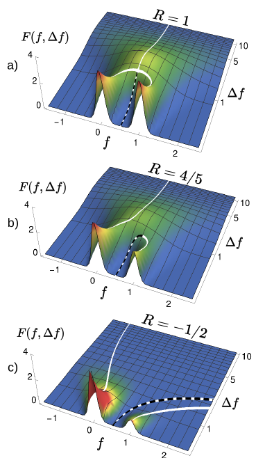
Figure 6: Maxima (solid) and minima (dashed) of $F(f)$ vs. $f$ and $\Delta f$ (a.u.). a) Pitchfork bifurcation for $R=1$, b) same as (a) but for $R=4/5$. c) same as (b) but for a negative $R=-1/2$. Note that in this case one has an “anomalous” value $z=-1$.

Appendix C The likelihood of discovering which way a classical system went

Consider a probability distribution,

$$\rho(f)=\frac{1}{2\Delta f\sqrt{\pi}}\left\{\exp\left[-\frac{f^{2}}{\Delta f^{2}}\right]+\exp\left[-\frac{(f-c)^{2}}{\Delta f^{2}}\right]\right\},\quad\quad$$ (44)

with $c>0$, and search for a range of $f$, where the first term can be neglected, compared to the second one. For example, one may look for readings where the ratio between the two terms does not exceed some $\epsilon\ll 1$. Such readings would occur for $f>f_{\epsilon}$, where $f_{\epsilon}=\Delta f^{2}|\ln\epsilon|/2c+c/2.$ The probability of finding a reading of this kind is, therefore, $P(f>f_{\epsilon})=\int_{f_{\epsilon}}^{\infty}\rho(f)df$. Replacing $\exp\left[-\frac{f^{2}}{\Delta f^{2}}\right]$ by a larger term $\exp\left[-\frac{(f-c)^{2}}{\Delta f^{2}}\right]$, we have [$\text{erfc}(x)$ is the complementary error function ABRAM ]

$$P(f>f_{\epsilon})<2^{-1}\text{erfc}\left[\frac{f_{\epsilon}-c}{\Delta f}\right]{\xrightarrow[\Delta f\to\infty]{}}$$ (45)

$$\frac{c}{2\sqrt{\pi}\Delta f|\ln\epsilon|}\exp\left[-\frac{\Delta f^{2}|\ln\epsilon|^{2}}{4c^{2}}\right]\to 0$$ .

The probability of finding a value $f$, which can be attributed to only one of the two terms in Eq.(44), vanishes rapidly for $\Delta f\gg c$.

Appendix D More properties of Gaussian distributions

Consider next a function

$$F(f)=\left|A\exp\left[-\frac{(f-a)^{2}}{\Delta f^{2}}\right]+B\exp\left[-\frac{(f-b)^{2}}{\Delta f^{2}}\right]\right|^{2}$$ (46)

with complex valued $A$ and $B$, and real $a$ and $b$

$$A=A_{R}+iA_{I},\quad B=B_{R}+iB_{I}.$$ (47)

Equation (46) can be rewritten as

$$F(f)=\left\{A_{R}\exp\left[-\frac{(f-a)^{2}}{\Delta f^{2}}\right]+B_{R}\exp\left[-\frac{(f-b)^{2}}{\Delta f^{2}}\right]\right\}^{2}$$

$$+\left\{A_{I}\exp\left[-\frac{(f-a)^{2}}{\Delta f^{2}}\right]+B_{I}\exp\left[-\frac{(f-b)^{2}}{\Delta f^{2}}\right]\right\}^{2}.$$ (48)

Applying (36) to each term in the curly brackets, and then to the sum of the results, yields

$$F(f){\xrightarrow[\Delta f\to\infty]{}}\tilde{F}(f)=|A+B|^{2}\exp\left[-2\frac{(f-\text{Re}[z])^{2}}{\Delta f^{2}}\right],$$ (49)

with $z$ still given by Eq.(35), but with complex valued $A$ and $B$,

$$z=\frac{a(A_{R}+iA_{I})+b(B_{R}+iB_{I})}{(A_{R}+B_{R})+i(A_{I}+B_{I})}.$$ (50)

Extension to two dimensions can be done in a similar manner as in Appendix A. For $\vec{f}=(f_{1},f_{2})$, $\vec{a}=(a_{1},a_{2})$ and $\vec{b}=(b_{1},b_{2})$

$$F(\vec{f})=\left|A\exp\left[-\frac{(\vec{f}-\vec{a})^{2}}{\Delta f^{2}}\right]+B\exp\left[-\frac{(\vec{f}-\vec{b})^{2}}{\Delta f^{2}}\right]\right|^{2}.\quad$$ (51)

we find

$$F(\vec{f}){\xrightarrow[\Delta f\to\infty]{}}|A+B|^{2}\exp\left[-2\frac{(\vec{f}-\text{Re}[\vec{z}])^{2}}{\Delta f^{2}}\right],$$ (52)

where $\vec{z}$ is still given by Eq.(42) with complex valued $A$ and $B$.

References

• (1) R. P. Feynman, R. Leighton and M. Sands, The Feynman Lectures on Physics III (Dover Publications, Inc., New York, 1989).
• (2) J. Von Neumann, Mathematical Foundations of Quantum Mechanics (Princeton University Press, Princeton, 1955), pp. 183-217, Chap. VI.
• (3) L. Vaidman, Past of a quantum particle, Phys. Rev. A 87, 052104 (2013).
• (4) A. Danan, D. Farfurnik, S. Bar-Ad, and L. Vaidman, Asking photons where they have been, Phys. Rev. Lett. 111, 240402 (2013).
• (5) P. L. Saldanha, Interpreting a nested Mach-Zehnder interferometer with classical optics, Phys. Rev. A 89, 033825 (2014).
• (6) R. B. Griffiths, Particle path through a nested Mach-Zehnder interferometer, Phys. Rev. A 94, 032115 (2016).
• (7) D. Sokolovski, Asking photons where they have been in plain language, Phys. Lett. A 381, 227 (2014).
• (8) Y. Aharonov, S. Popescu, D. Rohrlich, and P. Skrzypczyk, Quantum cheshire cats, New. J. Phys. 15, 113015 (2013).
• (9) T. Denkmayr, H. Geppert, S. Sponar, H. Lemmel, A. Matzkin, J. Tollaksen, and Y. Hasegawa, Observation of a quantum Cheshire Cat in a matter-wave interferometer experiment, Nat. Commun. 5, 4492 (2014).
• (10) Q. Duprey, S. Kanjilal, U. Sinha, D. Home, and A. Matzkin, The quantum cheshire cat effect: theoretical basis and observational implications, Ann. Phys. 391, 1 (2018).
• (11) D. Sokolovski, The meaning of ”anomalous weak values” in quantum and classical theories, Phys. Lett. A 379, 1097 (2015).
• (12) S. N. Sahoo, S. Chakraborti, S. Kanjilal, S. et al., Unambiguous joint detection of spatially separated properties of a single photon in the two arms of an interferometer, Commun. Phys. 6, 203 (2023).
• (13) R. P. Feynman, The Character of Physical Law (M.I.T. press, Cambridge, Mass, London, 1985).
• (14) Y. Aharonov, D. Albert, and L. Vaidman, How the result of a measurement of a spin component of the spin of a spin-1/2 particle can turn out to be 100, Phys. Rev. Lett. 60, 1351 (1988).
• (15) E. C. Zeeman, Catastrophe Theory: Selected Papers (Addison-Wesley Educational Publishers Inc, 1977).
• (16) X-s. Ma, J. Kofler, and A. Zeilinger, Delayed-choice gedanken experiments and their realizations , Rev. Mod. Phys. 88, 015005 (2016).
• (17) D. Sokolovski, D. Alonso Ramirez, and S. Brouard Martin, Speakable and unspeakable in quantum measurements, Ann. Phys. (Berlin) 535, 2300261 (2023).
• (18) R. P. Feynman, Simulating physics with computers, Int. J. Theor. Phys. 21, 467 (1982).
• (19) Handbook of Mathematical Functions, edited by M. Abramowitz and I. A. Stegun (Harri Deutsch, Thun, 1984).
Acknowledgements
D.S. acknowledges financial support by the Grant PID2021-126273NB-I00 funded by MICINN/AEI/10.13039/501100011033 and by ”ERDF A way of making Europe”, as well as by the Basque Government Grant No. IT1470-22.
A.U. and E.A. acknowledge the financial support by MICIU/AEI/10.13039/501100011033 and FEDER, UE through BCAM Severo Ochoa accreditation CEX2021-001142-S / MICIU/ AEI / 10.13039/501100011033; “PLAN COMPLEMENTARIO MATERIALES AVANZADOS 2022-2025 “, PROYECTO $\text{N}^{\text{o}}$:1101288 and grant PID2022-136585NB-C22; as well as by the Basque Government through ELKARTEK program under Grants KK-2023/00017, KK-2024/00006 and the BERC 2022-2025 program. This work was also supported by the grant BCAM-IKUR, funded by the Basque Government by the IKUR Strategy and by the European Union NextGenerationEU/PRTR.