Stability and dynamics of massive vortices in two-component Bose-Einstein condensates

Abstract

The study of structures involving vortices in one component and bright solitary waves in another has a time-honored history in two-component atomic Bose-Einstein condensates. In the present work, we revisit this topic extending considerations well-past the near-integrable regime of nearly equal scattering lengths. Instead, we focus on stationary states and spectral stability of such structures for large values of the inter-component interaction coefficient. We find that the state can manifest dynamical instabilities for suitable parameter values. We also explore a phenomenological, yet quantitatively accurate upon suitable tuning, particle model which, in line also with earlier works, offers the potential of accurately following the associated stability and dynamical features. Finally, we probe the dynamics of the unstable vortex-bright structure, observing an unprecedented, to our knowledge, instability scenario in which the oscillatory instability leads to a patch of vorticity that harbors and eventually ejects multiple vortex-bright structures.

I Introduction

The platform of atomic Bose-Einstein condensates (BECs) has been particularly fruitful towards the exploration of nonlinear wave patterns, both solitonic ones, as well as vortical ones involving topological charge Pethick and Smith (2002); Stringari and Pitaevskii (2003); Pitaevskii and Stringari (2003). The ability to manipulate external potentials in both space and time Henderson et al. (2009), as well as that of controlling the size and the sign of the atomic scattering length (and hence the coefficient of nonlinear interaction) in time Donley et al. (2001); Pollack et al. (2009) or even in space Kartashov et al. (2011); Di Carli et al. (2020) have paved new directions of unprecedented perturbations and dynamics to the solitary wave patterns that such systems can support.

In addition to the spatio-temporal control and the wealth of phenomenology of one-component atomic systems, two-component ones Kevrekidis et al. (2015); Kevrekidis and Frantzeskakis (2016) are, arguably, even richer in their potential phenomenology. On the other hand, the exploration of spinor systems Kawaguchi and Ueda (2012); Stamper-Kurn and Ueda (2013) has enabled the consideration of magnetic, as well as non-magnetic structures Li et al. (2005); Zhang et al. (2007); Nistazakis et al. (2008); Szankowski et al. (2011); Romero-Ros et al. (2019); Chai et al. (2020, 2021); Bersano et al. (2018); Fujimoto et al. (2019). These also include spin domains Miesner et al. (1999); Świsłocki and Matuszewski (2012) and spin textures Ohmi and Machida (1998); Song et al. (2013), taking advantage of the spin degree of freedom. In this setting, the ground state has been recognized to have the potential for antiferromagnetism in ²³Na or ferromagnetism in ⁸⁷Rb. However, perhaps even more interestingly, the wealth of such systems lies in the excited and topological structures that they can support in the three-component $F\!=\!1$ and the five-component $F\!=\!2$ settings Kawaguchi and Ueda (2012); Stamper-Kurn and Ueda (2013).

While these higher-component settings offer considerable additional wealth in terms of the possible states, our aim herein is to revisit two-component settings. There, many solitary waveforms have been considered, ranging from dark-bright (DB) to dark-dark and dark-antidark, as well as magnetic solitons Kevrekidis et al. (2015); Kevrekidis and Frantzeskakis (2016); Qu et al. (2016). Not only individual structures of this kind have been experimentally explored, but also small clusters thereof (see, e.g., Ref. Katsimiga et al. (2020)), as well as their collisions Becker et al. (2008). Such two-component settings have recently been leveraged also towards engineering effective attractive interactions in both 1D and 2D, offering the possibility to generate structures such as the Townes soliton Bakkali-Hassani et al. (2021), as well as the Peregrine soliton Romero-Ros et al. (2024).

Here, we focus on the 2D variants of the above solitary waves in the form of vortex-bright (VB) solitons Skryabin (2000); Law et al. (2010). These are sometimes referred to by other names such as baby-skyrmions, filled-core vortices, or massive vortices and have not only been theoretically explored but also experimentally observed Anderson et al. (2000); Leanhardt et al. (2003); Choi et al. (2012). Note that some of these experimental realizations such as the one reported in Ref. Choi et al. (2012) (and corresponding theoretical explorations such as in Ref. Katsimiga et al. (2023)) have probed these states in spinor settings. In recent years there has been a flurry of activity in such systems, seeking to provide a theoretical understanding of the potential dynamics of these structures. Indeed, they have been shown to be able to perform flower-like motions Richaud et al. (2021); Caldara et al. (2023); they have been also explored in generalized radial potentials Wang (2022); Richaud et al. (2022), as well as in the context of rotating traps Richaud et al. (2020) and more recently the case of multiple such states and how they interact has been revisited Richaud et al. (2023) (see also earlier studies in Refs. Pshenichnyuk (2018); Kasamatsu et al. (2016)).

Here, our aim is to complement some of these developments, which have chiefly been based on Lagrangian (variational) analytical formulations and direct numerical simulations, by means of steady state computations, Bogoliubov-de Gennes (BdG) stability analysis, dynamics, and a modified ODE analytical framework. In Sec. II, we provide a palette of relevant tools upon discussing the model. Notice that here we are primarily focusing on scenarios that are deep within the immiscible regime, in line with some of the above works, e.g., by Richaud and collaborators Richaud et al. (2021); Caldara et al. (2023); Richaud et al. (2022, 2023). We also discuss the details of an analytical approach that has some modified features in comparison to the above works. We analyze the types of motions that are permissible in this reduced system and provide their quantitative characteristics towards a comparison with the full numerical PDE results. In Sec. III, we provide the numerical continuation of our VB states as a function of the system’s chemical potentials for different values of the inter-species coupling. Here, we also offer a systematic procedure for matching the ODE and PDE dynamics, and showcase that this matching is also reflected in the BdG spectrum of the VB matching the corresponding particle model eigenfrequencies. Moreover, we trace an (oscillatory) instability of the PDE VB state when two pertinent eigenfrequencies collide and become complex. These findings, in turn, prompt us to perform select dynamics, reflecting some of the more elaborate VB features, such as the flower-like trajectories thereof, but also the instabilities of such structures. The latter turn out to be especially intriguing as the oscillatory instability results in the formation of a patch of vorticity harboring multiple VB structures that eventually lead to a breakup of the relevant pattern in different segments. Finally, in Sec. IV, we summarize our findings and present our conclusions.

II Model and Theoretical Setup

II.1 Full PDE model

To study the existence, stability, and dynamics of VB complexes, let us consider the 2D Gross-Pitaevskii (GP) equation describing the interaction between two different atomic species in a BEC. The corresponding GP equation can be cast in non-dimensional form as:

$$i\dot{\Psi}_{1} = \displaystyle-\frac{1}{2}\Delta\Psi_{1}+\left[V(r)+|\Psi_{1}|^{2}+g_{12}|\Psi_{2}|^{2}\right]\Psi_{1},~{}~{}~{}~{}$$ (1a)

$$i\dot{\Psi}_{2} = \displaystyle-\frac{1}{2}\Delta\Psi_{2}+\left[V(r)+|\Psi_{2}|^{2}+g_{12}|\Psi_{1}|^{2}\right]\Psi_{2},~{}~{}~{}~{}$$ (1b)

where both BEC wavefunction species $\Psi_{1}$ and $\Psi_{2}$ are confined by the common external parabolic potential $V(r)=\frac{1}{2}\Omega^{2}r^{2}$ with strength $\Omega$ which is usually deployed in the experiments using a magnetic field Stringari and Pitaevskii (2003); Pethick and Smith (2002); Kevrekidis et al. (2015). Here, $\Delta$ denotes the 2D Laplacian, the overdot is used for differentiation with respect to time, and $g_{12}>0$ is the adimensional inter-species coupling. It is relevant to point out here that we have in mind a setup such as ⁸⁷Rb (or similar) in which the intra-species scattering lengths are practically equal, while we think of the inter-species one as being tunable via external fields Stringari and Pitaevskii (2003); Kevrekidis et al. (2015). To construct VB complexes we consider the first component to be populated with a relatively large number of atoms so that it is close to its Thomas-Fermi (TF) limit. We will dub this component the “dark” component as it will be primarily governed by the self-repulsive interaction present in the first component [cf. positive sign in front of $|\Psi_{1}|^{2}$ in Eq. (1a)] and it will be featuring a vortex structure. In turn, the vortex embedded in the dark component will induce an effective potential on the second component through the term $g_{12}|\Psi_{1}|^{2}\Psi_{2}$ in Eq. (1b) that will trap a relatively small number of atoms and create a localized hump that we will dub the “bright” component. This is the origin of the terminology associated with the vortex-bright (or dark-bright in 1D Kevrekidis and Frantzeskakis (2016)) complex. Solutions to Eq. (1) conserve the atom number (power) in each of the two components:

$$P_{j}=\iint_{-\infty}^{+\infty}|\psi_{j}|^{2}\,dx\,dy\quad{\rm for}\quad j=1,2.$$ (2)

An additional important parameter for the VB complex is the —also conserved— mass ratio:

$$M=\frac{P_{2}}{P_{1}}.$$ (3)

Let us now seek stationary state solutions of the form $\Psi_{1}(x,y,t)=\psi_{1}(x,y)\,e^{-i\mu_{d}t}$ and $\Psi_{2}(x,y,t)=\psi_{2}(x,y)\,e^{-i\mu_{b}t}$ where $\mu_{d}$ and $\mu_{b}$ denote the chemical potentials of the dark and bright components, respectively. Then, the spatial part of the stationary solutions satisfies

$$-\frac{1}{2}\Delta\psi_{1}+\left[V(r)+|\psi_{1}|^{2}+g_{12}|\psi_{2}|^{2}-\mu_{d}\right]\psi_{1} = 0,~{}~{}~{}~{}$$ (4a)

$$-\frac{1}{2}\Delta\psi_{2}+\left[V(r)+|\psi_{2}|^{2}+g_{12}|\psi_{1}|^{2}-\mu_{b}\right]\psi_{2} = 0.~{}~{}~{}~{}$$ (4b)

The VB states are studied in the parameter space. Here, the key parameters determining the properties of the VB complex are $\Omega$, $g_{12}$, $\mu_{d}$, and $\mu_{b}$. For example, the powers and the mass ratio depend directly, in a non-trivial manner, on the chemical potentials for a given set of $\Omega$ and $g_{12}$ values.

We find numerically exact stationary states using finite differencing for the spatial discretization together with a Newton-based fixed-point iteration method. First, we find a relevant solution, and then numerical continuation can be deployed along any of the above parameters. The first solution is obtained by embedding a vortex centered at the origin in the first component, we shall discuss the details in Sec. III. We also study the (spectral) stability of these centered VB complexes by the BdG analysis. Then, taking parameter values where the VB complex is stable, we proceed to appropriately seed it away from the trap center and monitor, according to Eq. (1), its dynamical evolution. Our dynamics is carried out using the regular fourth-order Runge-Kutta method. The location of the VB complex is monitored by computing the respective centers of mass of each component along the $x$ and $y$ directions:

$${\rm CoM}^{\sigma}_{j}=\frac{1}{P_{j}}\iint_{-\infty}^{+\infty}\sigma|\Psi_{j}|^{2}\,dx\,dy,$$ (5)

where $\sigma=x,y$. Then, the relative location of the VB with respect to the background cloud of the dark component is recorded.

The BdG analysis for the two-component stationary solutions works as follows. Given the steady state solutions $(\psi_{1},\psi_{2})$ as per Eq. (4), we perturb them according to

$$\Psi_{1} = \left\{\psi_{1}+\varepsilon\left[a_{1}(x,y)e^{\nu t}+b_{1}^{*}(x,y)e^{\nu^{*}t}\right]\right\}e^{-i\mu_{d}t},~{}~{}~{}$$

$$\Psi_{2} = \left\{\psi_{2}+\varepsilon\left[a_{2}(x,y)e^{\nu t}+b_{2}^{*}(x,y)e^{\nu^{*}t}\right]\right\}e^{-i\mu_{b}t}.~{}~{}~{}$$

The spectra are then computed by plugging Eq. (LABEL:eq:perturb) into Eq. (1) and solving the resulting linearized eigenvalue problem at order $\varepsilon$ as:

$$-i\left[\begin{array}[]{cccc}\phantom{-}M_{11}&\phantom{-}M_{12}&\phantom{-}M_{13}&\phantom{-}M_{14}\\ -M_{12}^{*}&-M_{11}^{*}&-M_{14}^{*}&-M_{13}^{*}\\ \phantom{-}M_{13}^{*}&\phantom{-}M_{14}&\phantom{-}M_{22}&\phantom{-}M_{34}\\ -M_{14}^{*}&-M_{13}&-M_{34}^{*}&-M_{22}^{*}\\ \end{array}\right]\left[\begin{array}[]{c}a_{1}\\ b_{1}\\ a_{2}\\ b_{2}\end{array}\right]=\nu\left[\begin{array}[]{c}a_{1}\\ b_{1}\\ a_{2}\\ b_{2}\end{array}\right],$$ (7)

where

$$M_{11} \equiv -\frac{1}{2}\Delta+V-\mu_{d}+2|\psi_{1}|^{2}+g_{12}|\psi_{2}|^{2},$$

$$M_{22} \equiv -\frac{1}{2}\Delta+V-\mu_{b}+2|\psi_{2}|^{2}+g_{12}|\psi_{1}|^{2},$$

and $M_{12}\equiv\psi_{1}^{2}$, $M_{13}\equiv g_{12}\psi_{1}\psi_{2}^{*}$, $M_{14}\equiv g_{12}\psi_{1}\psi_{2}$, and $M_{34}\equiv\psi_{2}^{2}$. The eigenvector for the corresponding eigenvalue $\nu$ is $[\Psi_{1},\Psi_{2}]^{T}=[(a_{1},b_{1}),(a_{2},b_{2})]^{T}$, and the mode is unstable if Re$(\nu)>0$. As we will see in Sec. III, after stationary solutions are displaced away from the origin and for appropriate parameter regimes, the VB states can exhibit flowering trajectories whose two main frequencies are approximated by the pertinent eigenvalues of the corresponding BdG spectrum. In order to follow potential instabilities emerging from the collision of eigenvalues, for each eigenvector we monitor the sign of the quantity (so-called Krein signature) Kapitula et al. (2004):

$$K=\iint_{-\infty}^{+\infty}(|a_{1}|^{2}-|b_{1}|^{2}+|a_{2}|^{2}-|b_{2}|^{2})\,dx\,dy.$$ (9)

Collision of two dynamically stable [Re$(\nu)=0$] eigenvalues of opposite Krein sign generically leads to an oscillatory instability Skryabin (2000). In Sec. III we detail the presence of a supercritical Hamiltonian Hopf bifurcation when continuing along the $\mu_{b}$ parameter. This is induced precisely by the collision of two opposite Krein sign eigenvalues that correspond to the observed flowering frequencies of the VB evolution; see more details on that below.

II.2 Reduced ODE model for the VB complex

We now turn to a theoretical description of the particle motion of the VB structure inside the parabolic trap. This will provide a yardstick of comparison for the parametric dependence of the PDE results that will be obtained below based on the methods presented in Sec. II.1. Our model somewhat differs from the one used, e.g., in Ref. Richaud et al. (2021) in the following two ways. The latter model contains a singular logarithmic term in its potential energy, while the model used herein contains an effective potential energy essentially proportional to the system density at the location of interest (see details below). Furthermore, the term giving rise to the Magnus force and being effectively associated with the angular momentum also emerges linearly in its dependence on the density (leading to the right equation in the single-component vortex limit). In that vein, based on the above motivations, we follow the approach of Ref. Ruban (2022), using effectively as the dynamical model of relevance the one of Eq. (29) therein.

The ODE model can be reduced to the following second order system on the VB position $(x(t),y(t))$:

$$M_{0}\,\ddot{x} = \frac{\Lambda}{2}x-\rho(r)\dot{y}$$

(10)

$$M_{0}\,\ddot{y} = \frac{\Lambda}{2}y+\rho(r)\dot{x}$$

where $M_{0}$ and $\Lambda$ depend, in a non-trivial manner, on the relative mass $M$ and the inter-species coupling $g_{12}$ Ruban (2022), and $\rho(r)\equiv\mu_{d}-V(r)$ is the TF background density of the dark component. The equations of motion can be recovered through the Euler-Lagrange equations $\frac{d}{dt}\left(\frac{\partial L}{\partial\dot{\sigma}}\right)=\frac{\partial L}{\partial\sigma}$, for $\sigma=x,y$, from the corresponding Lagrangian:

$$L=\frac{M_{0}}{2}(\dot{x}^{2}+\dot{y}^{2})-\frac{1}{2}(x\dot{y}-y\dot{x})\left(\mu_{d}-\frac{1}{2}V(r)\right)+\frac{\Lambda}{4}r^{2}.$$ (11)

Note that we may also write $L$ in polar coordinates using standard conversion formulas $x^{2}+y^{2}=r^{2}$, $\dot{x}^{2}+\dot{y}^{2}=\dot{r}^{2}+r^{2}\dot{\theta}^{2}$, and $x\dot{y}-y\dot{x}=r^{2}\dot{\theta}$ for $r=r(t)$ and $\theta=\theta(t)$. Comparing Eq. (11) above with the Lagrangian (23) of Ref. Richaud et al. (2021), we find similar structural features with the expression used herein bearing an additional contribution $\left[\mu_{d}-\frac{1}{2}V(r)\right]$ in the second kinetic energy term, while instead of their logarithm, we include herein only the quadratic term in its Taylor series. Additionally, their $r$ is normalized as $r/R_{\rm TF}$ for $R_{\rm TF}$ the TF radius of the dark component.

The conservation of angular momentum in polar coordinates can be inferred from the angular Euler-Lagrange equation $\frac{d}{dt}\left(\frac{\partial L}{\partial\dot{\theta}}\right)=\frac{\partial L}{\partial\theta}$ which yields:

$$\ell=\Omega^{2}M_{0}r^{2}\dot{\theta}+\frac{1}{2}\rho^{2}(r).$$ (12)

On the other hand, to derive the Hamiltonian formulation of the ODE system (10) we can utilize the Legendre transform $H=\dot{x}\rho_{x}+\dot{y}\rho_{y}-L$ with $\rho_{\sigma}=\frac{\partial L}{\partial\dot{\sigma}}$ for $\sigma=x,y$, to obtain

$$H = \frac{1}{2M_{0}}\left(\rho_{x}^{2}+\rho_{y}^{2}-(y\rho_{x}-x\rho_{y})\left(\mu_{d}-\frac{1}{2}V(r)\right)\right)$$ (13)

$$+\frac{r^{2}}{8M_{0}}\left(\mu_{d}-\frac{1}{2}V(r)\right)-\frac{\Lambda}{4}r^{2}.$$

The effective total (and conserved) energy can then be written as follows:

$$E=\frac{1}{2}M_{0}\dot{r}^{2}+V_{\rm eff}(r),$$ (14)

with the effective potential

$$V_{\rm eff}(r)=\frac{1}{2}M_{0}r^{2}\dot{\theta}^{2}-\frac{\Lambda}{4}r^{2}.$$ (15)

Using Eq. (12) to replace $\dot{\theta}^{2}$ with the corresponding expression in terms of $\ell$ we can also write the effective potential as:

$$V_{\rm eff}(r)=\frac{1}{2\Omega^{4}M_{0}r^{2}}\left(\ell-\frac{1}{2}\rho(r)^{2}\right)^{2}-\frac{\Lambda}{4}r^{2}.$$ (16)

The Euler-Lagrange equation in the radial variable $\frac{d}{dt}\left(\frac{\partial L}{\partial\dot{r}}\right)=\frac{\partial L}{\partial r}$ yields:

$$M_{0}(\ddot{r}-r\dot{\theta}^{2})=-\rho(r)r\dot{\theta}+\frac{\Lambda}{2}r,$$ (17)

which can be used to derive the expected precessional frequency of a circular trajectory by setting $r=r_{0}$ and $\ddot{r}=0$ to obtain the quadratic-in-$\dot{\theta}$ equation

$$0=M_{0}\dot{\theta}^{2}-\rho(r_{0})\dot{\theta}+\frac{\Lambda}{2}.$$ (18)

Solving for $\dot{\theta}$ yields frequencies

$$\dot{\theta}_{\pm}=\frac{1}{2M_{0}}\left(\rho(r_{0})\pm\sqrt{\rho(r_{0})^{2}-2M_{0}\Lambda}\right).$$ (19)

The smaller frequency $\omega_{\rm pr}\equiv\dot{\theta}_{-}$ corresponds to the expected precessional frequency of a circle, but we also obtain the larger frequency $\dot{\theta}_{+}$ that corresponds to the radial or flowering frequency.

For simplicity, we assume that a circle begins with $x(0)=x_{0}$, $y(0)=0$, and $\dot{x}(0)=0$. This yields, according to Eq. (18) converted to Cartesian coordinates, the initial velocity for a circle in the ODE model as:

$$\dot{y}(0)=\frac{1}{2M_{0}}\left(\rho(r_{0})x_{0}\pm\sqrt{\rho(r_{0})^{2}x_{0}^{2}-2M_{0}\Lambda r_{0}^{2}}\right).$$ (20)

Finally, we note that the resulting frequencies of flowering trajectories can be estimated by converting the conservation Eqs. (12)–(14) into a first order system and linearizing as follows. First off, the potential flowering pertains to small oscillations in the radial direction around an equilibrium circular trajectory $r=r_{0}$. Differentiating Eq. (14) and solving for $\dot{\theta}$ in Eq. (12) we can write the system as $\dot{r}=u$, $\dot{u}=\ddot{r}=G(r)$, and $\dot{\theta}=K(r)$ for

$$G(r) \equiv -V^{\prime}_{\rm eff}(r)/M_{0}$$

$$K(r) \equiv \frac{1}{\Omega^{2}M_{0}r^{2}}\left(\ell-\frac{1}{2}\rho(r)^{2}\right).$$

Near the minimum $r_{0}$ of $V(r)$ we estimate

$$r(t) \approx r_{0}+R\cos(\omega_{r}t)$$

$$\theta(t) = \omega_{\rm pr}t+A_{0}\sin(\omega_{r}t)$$

for radial and precesional frequencies $(\omega_{r},\omega_{\rm pr})$ and $R$ and $A_{0}$ being small perturbations off of the circular motion. Plugging Eqs. (LABEL:eq:estRTheta) into the first order system above gives

$$\omega_{r}^{2} = \frac{V^{\prime\prime}_{\rm eff}(r_{0})}{M_{0}},$$

$$A_{0} = \frac{RK^{\prime}(r_{0})}{\omega_{r}},$$

for $R=r(0)-r_{0}$. Note that, according to Eqs. (LABEL:eq:estRTheta), flowering trajectories with looping petals occur when ${\rm min}\{\dot{\theta}(t)\}=\omega_{\rm pr}-\omega_{r}A_{0}$ is negative so that looping appears at the threshold amplitude $A_{0}=\omega_{\rm pr}/\omega_{r}$ according to the linearized prediction.

In the next section, we will make the correspondence between the PDE model and its effective ODE reduction using the following program. Since we expect frequencies $\dot{\theta}$ from the ODE model to correspond to purely imaginary frequencies in the PDE model, we use the BdG bifurcating eigenvalues $\nu$ and the correspondence $\dot{\theta}={\rm Im}(\nu)$ in order to estimate the ODE parameter value of $\Lambda$ in terms of $M_{0}$. The value of $M_{0}$ is then determined by minimizing the sum of squares of differences between the PDE and ODE trajectories. For a given pair of $M_{0}$ and $\Lambda$ one then finds initial velocities of the ODE model that best align to a given PDE trajectory. In general, a larger initial velocity gives flowering trajectories with more looping on the petals so this can be used to guide best choices of these initial velocities in the ODE. For the obtained flowering trajectories, we will also show examples to compare the ODE trajectories according to Eq. (10) versus the results of the linearized predictions in Eqs. (LABEL:eq:estRTheta) and (LABEL:eq:omegaA).

III Results

III.1 Steady states and stability for the PDE model

To obtain the stationary solutions of Eq. (4), the ground state cloud $(\psi_{1},\psi_{2})=(\psi_{\rm gs},0)$ for the isolated dark component is found via a standard fixed point Newton’s iteration method with an initial guess corresponding to the TF approximation $\psi_{1}=\sqrt{\max(\mu_{d}-V(r),0)}$. In turn, to find a VB solution of Eq. (4) centered at the origin, we again use Newton’s method, this time with the initial guess in the bright component as $\psi_{2}=\sqrt{\mu_{b}}\,\rm sech(\mu_{b}r)$ and in the dark component as $\psi_{1}=\psi_{\rm gs}\tanh(\mu_{d}r)e^{-i\theta(x,y)}$ where $\theta$ is the (polar) angle of $(x,y)$ from the origin. The resulting unit (negative) charge VB stationary centered solutions exist for a variety of combinations of the parameters $\Omega$, $g_{12}$, $\mu_{b}$, and $\mu_{d}$. Once a relevant solution is found, it can be further continued along any of these parameters. Similarly, if we take the complex conjugate of the initial guess, we can obtain a VB state with an opposite charged vortex.

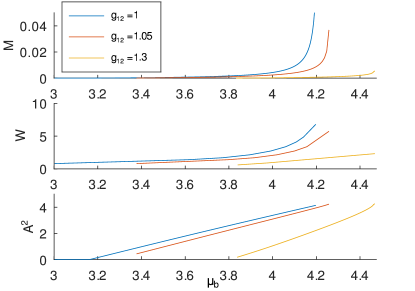
Figure 1: Static properties of the VB steady state centered at the origin. From top to bottom: mass ratio $M$, full width at half max $W$, and squared amplitude $A^{2}$ of the bright component. These properties are plotted for relatively small values of the inter-species coupling $g_{12}$ for fixed values of $\mu_{d}=4.22$ and $\Omega=0.1$. For these relatively small values of $g_{12}$, all properties increase with increasing $g_{12}$.

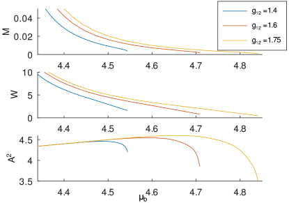
Figure 2: Same as Fig. 1 but for higher $g_{12}$ values.

We monitor three properties of the stationary VB states: the full width half max (FWHM) $W$, the squared amplitude $A^{2}$ of the bright component, and the mass ratio $M$ of the two components as defined in Eq. (3). These properties are computed along a continuation in $\mu_{b}$ for fixed values of $g_{12}$, $\mu_{d}$, and $\Omega$, and they are depicted in Figs. 1 and 2. For the relatively small values of $g_{12}$ closer to $1$ shown in Fig. 1, increasing $\mu_{b}$ results in a larger mass ratio $M$, larger FWHM $W$, and larger amplitude $A$. In this regime, higher mass ratio solutions are wider and taller. In contrast, for the relatively larger values of $g_{12}$ shown in Fig. 2, namely farther into the immiscible regime, it is the lower $\mu_{b}$ values that correspond to higher mass ratio $M$, and as $\mu_{b}$ decreases this corresponds to an inverse relation between $A$ and $W$ (cf. as width increases, the amplitude decreases). In this regime, higher mass ratio solutions are wider but also shorter. In Fig. 3 we depict two typical examples of the densities of the VB complex stationary solution, one in each of the above-mentioned regimes. Figure 4 shows the corresponding density cross sections. Figures 3 and 4 tend to suggest that, for the same mass ratio $M$, bright spots in the lower $g_{12}$ regime are tapered at the top with a wide base (appearing with soft edges) while bright spots in the higher $g_{12}$ regime appear less tapered (sharper with more well-defined boundaries). This is rather intuitive on account of the deeper immiscibility region arising as $g_{12}\gg 1$.

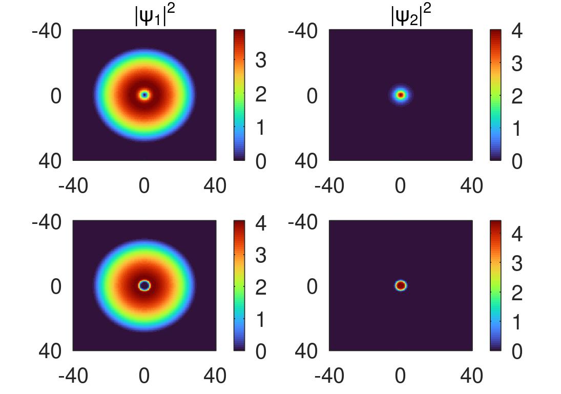
Figure 3: Vortex-bright complexes. Depicted are the densities of two steady state solutions with parameter values $\Omega=0.1$ and $\mu_{d}=4.22$ where both solutions have mass ratio $M\approx 0.02$. The top row solution corresponds to $(g_{12},\mu_{b})=(1,4.16)$ and the solution appears to have soft edges with the bright spot having a wider footprint. By contrast, the bottom row solution corresponds to $(g_{12},\mu_{b})=(1.4,4.43)$ where the solution shows a sharper boundary with the bright spot featuring a slightly narrower footprint.

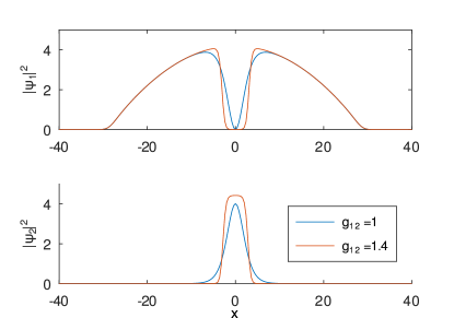
Figure 4: Cross sections of the solutions depicted in Fig. 3. The top (bottom) panel illustrates the dark (bright) component for the values of $g_{12}$ indicated.

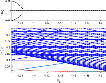
Figure 5: BdG stability spectrum for a VB structure centered at the origin as a function of $\mu_{b}$ for $g_{12}=1.6$, $\mu_{d}=4.25$, and $\Omega=0.1$. The top and bottom panels depict, respectively, the real and imaginary parts of the eigenvalues. A positive real part indicates instability. The eigenvalues are color-coded according to the sign of the Krein signature of the corresponding eigenvector: zero (black), negative (blue), and positive (red). The resulting bifurcation diagram evidences the presence of a (reverse) Hamiltonian Hopf bifurcation at $\mu_{b}\approx 4.383$. Overlaid are plots (cyan) of $\dot{\theta}$ values of the matching ODE given by Eq. (19).

Let us now track the BdG eigenvalue spectrum for the centered VB structure as a function of the parameter $\mu_{b}$. Figure 5 depicts a typical spectrum for $g_{12}=1.6$ and $\mu_{d}=4.25$. Note that Re$(\nu)>0$ indicates an instability. Interestingly, as the spectrum shows, there is a Hamiltonian Hopf bifurcation as $\mu_{b}$ decreases. For $\mu_{d}=4.25$ and values $g_{12}=1.4,1.6,1.75$, the bifurcations occur, respectively, at $\mu_{b}\approx 4.349,4.383,4.403$. This (reverse) Hamiltonian Hopf bifurcation evidences that the lowest two oscillatory (purely imaginary) eigenfrequencies collide as $\mu_{b}$ decreases giving rise to an unstable (complex) quartet. The presence of a complex quartet instability indicates that, in this parametric regime, the VB will destabilize from the center of the trap along an spiralling-out trajectory as we will see below soon. According to the color-coded eigenvalues in Fig. 5, the region of instability lies where the lower branch is colored black for $\mu_{b}\lesssim 4.383$. However, it is interesting that, with the parameters provided in Fig. 5, spiralling-out is also present for $\mu_{b}$ values as high as $\mu_{b}<4.4$ when the VB structure is displaced by a large value such as $x_{0}=2.5$. This tends to suggest that precessional circular orbits may also be prone to instabilities. This is a topic of particular interest in its own right, meriting an examination of such states in a co-rotating frame (as was done, e.g., in the work of Pelinovsky and Kevrekidis (2012)), yet this type of distinct study is an interesting topic for future work.

Focusing on initially centered VB solutions, according to our BdG spectral analysis, starting infinitesimally close to the center, spiral-out trajectories will only be present in the $\mu_{b}$-interval where the stationary solutions are unstable. For instance, the VB dynamics for an initial condition $(x_{0},y_{0})=(2.5,0)$ in the stable regime ($\mu_{b}\approx 4.4$) displays flowering trajectories that have roughly two petals and as $\mu_{b}$ increases the number of petals increase. In Fig. 5, we overlay the two frequencies obtained from the ODE model given by Eq. (19); see the two cyan curves. In the stable regime, these ODE frequencies correspond to the two eigenfrequencies emerging from the Hamiltonian Hopf bifurcation within the PDE model. Note the excellent agreement between these two BdG eigenfrequencies and their ODE counterparts. It is important to note that this agreement is valid for a relatively wide range of $\mu_{b}$ values since the fit of the ODE frequencies, and hence the fit of the parameters $M_{0}$ and $\Lambda$ in Eqs. (10), was performed for each value of $\mu_{b}$. Nonetheless, we checked that, for each chosen value of $\mu_{b}$ (and the corresponding fitted parameters), the PDE and ODE orbits matched for a wide range of initial conditions. This evidences the validity of the ODE model not only qualitatively, but more importantly, quantitatively in its ability to capture the VB evolution within the full PDEs once the parameters of the system are set.

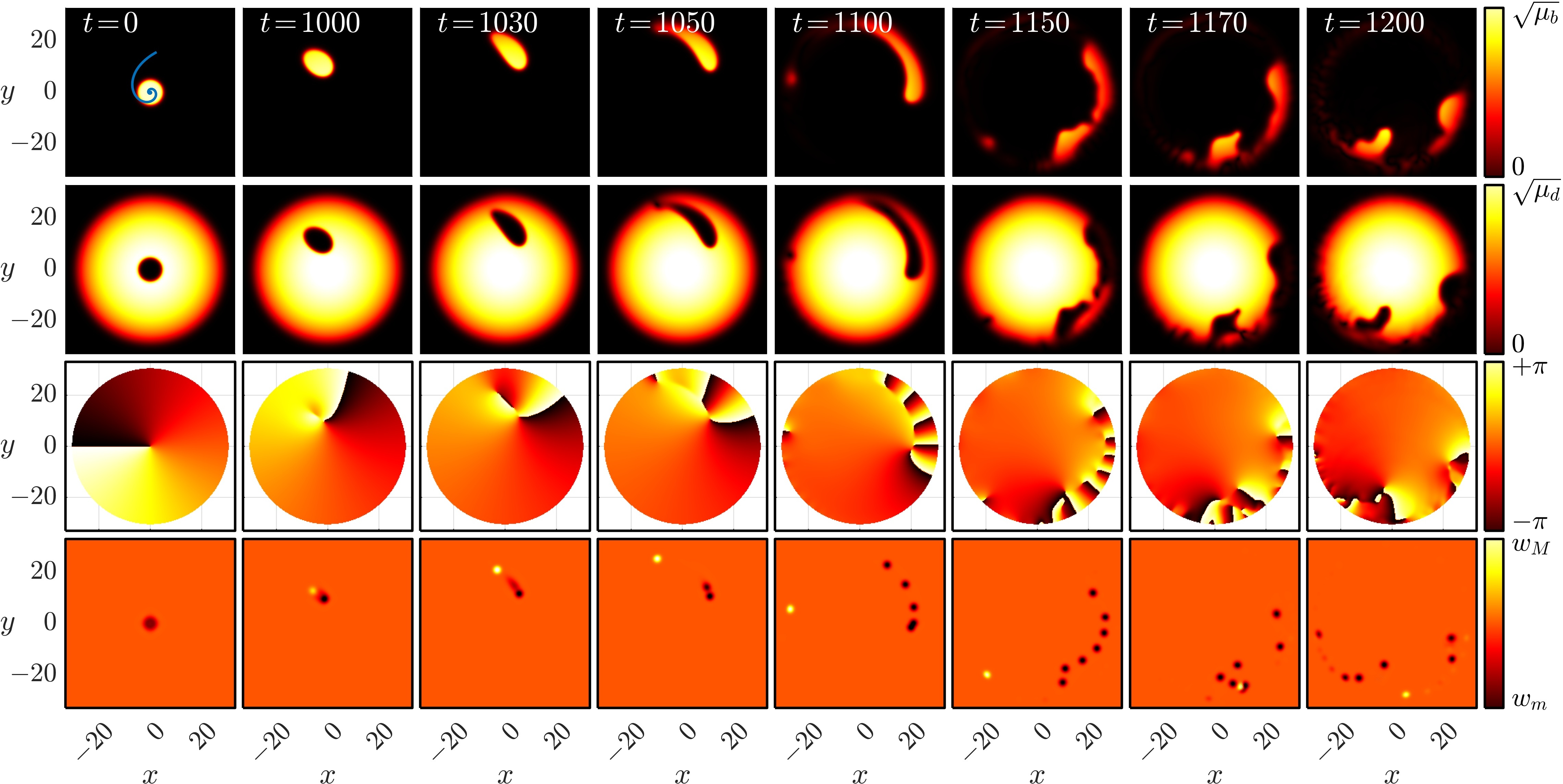
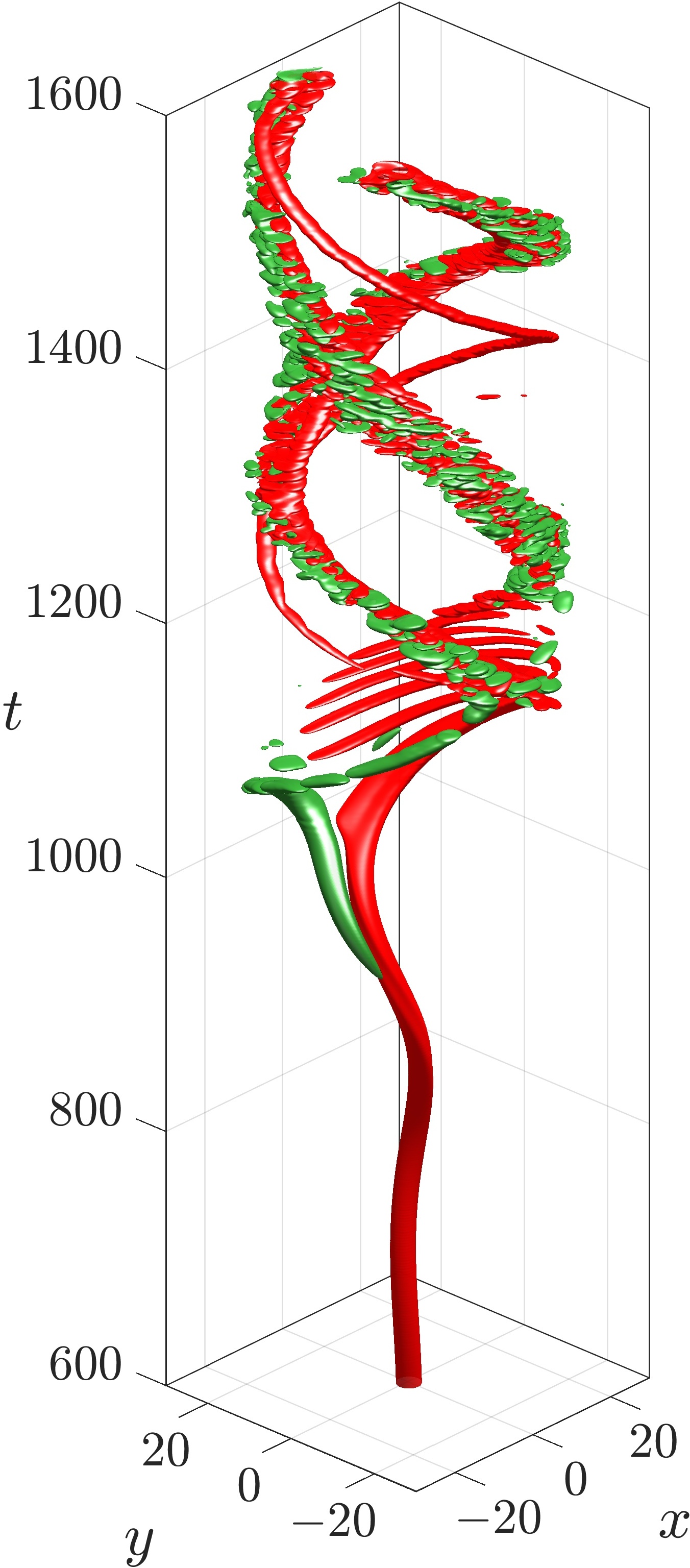
Figure 6: Evolution of an initially centered unstable VB structure for $\mu_{d}=4.25$ and $\mu_{b}\approx 4.38$. The first and second rows of panels depict the (squared root) of the densities for, respectively, the bright and dark components at the times indicated. The blue spiral in the top-left panel corresponds to the orbit followed by the VB structure during its destabilization for $0\leq t\leq 1000$. The third and fourth rows of panels depict, respectively, the phase and vorticity of the dark component. For convenience, the phase panels only show the region inside the Thomas-Fermi radius (outside this region the phases are very complicated as the density rapidly decays to zero). The yellow (black) dots in the vorticity panels depict the location of positively (negatively) charged vortices where the vorticity attains its maximum (minimum) denoted by $w_{M}$ ($w_{m}$). The right panel depicts the evolution of the vorticity by means of isocontours of vorticity in $(x,y,t)$ where the red and green contours correspond to negative and positive vorticities, respectively.

On the other hand, for our chosen parameters and as per our stability analysis, for $\mu_{b}<4.4$ the VB structure centered at the origin is unstable and tends to spiral out. We provide a typical example of the destabilization dynamics in this region in Fig. 6 which depicts the time-evolved solution together with its phase and vorticity profiles. As expected, for initial times ($t\lesssim 1000$), the VB destabilizes from the origin and performs a spiraling-out motion (see overlaid blue curve in the top-left panel) while, approximately, preserving its VB initial shape albeit a small elongation along the spiralling direction. Further down the evolution, this elongation of the VB “patch” becomes more pronounced allowing for the formation of extra vortices inside the VB. Initially, a vortex-anti-vortex pair creation occurs inside the VB complex (see the state at $t=1030$). Then, the corresponding negatively charged vortex keeps trapped within the VB complex while the positively charged vortex, carrying a small amount of bright mass, is ejected out of the VB and runs toward the edge of the condensate orbiting in the opposite direction of the VB motion. Next, as the VB patch continues to stretch, a series of aligned vortices of negative charge are created giving rise to a quasi-1D vortex “patch”. Eventually, the stretched VB patch breaks into two individual VB patches, each carrying a portion of the vortices. We note that, to the best of our knowledge, this intrinsic creation of vortices (i.e., without the need of an external stirrer or potential) is associated with a novel type of VB-creating instability. What seems to be happening here involves the transfer of angular momentum associated with the spiraling motion of the VB into net vorticity since the vortices produced are predominantly of the same charge.

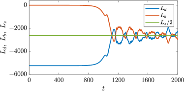
Figure 7: Temporal evolution of the angular momentum for the destabilization dynamics of an initially centered VB depicted in Fig. 6. The initial gradual angular momentum exchange starting around $t\approx 800$ corresponds to the spiralling-out of the VB. As time progresses, the angular momentum of each component tends to vary around the equipartition level $L_{d}\approx L_{b}\approx L_{z}/2$.

In order to garner more information about the emergence of new vortices through the above-mentioned destabilization dynamics of the centered VB complex, we monitor the vorticity in the system. In particular, the angular momentum in each component can be computed using Mukherjee et al. (2020):

$$L_{d,b}(t)=-i\iint_{-\infty}^{+\infty}\Psi^{*}_{d.b}\left(x\partial_{y}-y\partial_{x}\right)\Psi_{d,b}\,dx\,dy,$$ (24)

where the subscripts denote the first (dark) and second (bright) components. Since the underlying potentials for both components are independent of the angular coordinate, the total angular momentum of the system is conserved:

$$L_{z}(t)=L_{d}(t)+L_{b}(t)=L_{z}(0).$$ (25)

Figure 7 illustrates the evolution of the angular momentum for the destabilization dynamics of the initially centered VB complex described in Fig. 6. As we saw in Fig. 6, the VB complex evolves and creates vortices of different charges during its evolution. However, as Fig. 7 confirms, the total angular momentum is indeed conserved. It is interesting to note that the angular momentum transfer from the dark to the bright component seems to occur as a result of the spiral-out motion (which only starts to become significant after $t=800$). In this process, the bright soliton gains angular speed and moves further away from the origin as thus increasing $|L_{b}|$ at the expense of $|L_{d}|$.

Subsequently, as vortex nucleations and annihilations ensue, there is a back-and-forth exchange of angular momentum between the two components. Nonetheless, it is particularly interesting to note that in this case the system tends to “equilibrate” towards a state that has relatively small angular momentum exchanges between the components that hover around the mean value of the total angular momentum such that $L_{d}\approx L_{b}\approx L_{z}/2$. It would be interesting to study this apparent angular momentum equipartition between the components in systems with large number of vortices in the quantum turbulent regime. It is also relevant to point out that in Fig. 6, the majority of the vortices created feature a circulation in the negative direction. This is natural to expect given the selection of a spiraling direction of the vorticity patch upon the manifestation of the Hamiltonian Hopf bifurcation-related instability. In addition, this spiral direction is a result of the negatively charged vortex state, i.e., it is the same as the precessional direction of the initial VB state in the harmonic trap and can be reversed for vortices of opposite charge.

III.2 Vortex-bright dynamics

We now leverage the ODE reduction dynamics presented in Sec. II.2 to describe the dynamics of the VB in the original PDE model. To generate rotational dynamics of the VB state at the level of the original GP model (1), we displace the stationary solutions away from the origin and seed the waveform into a ground state cloud according to the following procedure. First we compute, using our fixed-point algorithm, the ground state cloud $\psi_{1}=\psi_{\rm gs}$ for a given chemical potential value $\mu_{d}$ and a fixed value of the inter-species coupling $g_{12}$ (while we keep the trap strength constant $\Omega=0.1$ throughout this analysis). For convenience we choose a starting point with $x(0)=x_{0}$ and $y(0)=0$. Next, we interpolate the local chemical potential $\mu_{x_{0}}=|\psi_{\rm gs}(x_{0},0)|^{2}$ where the VB will be seeded. The VB solution with $\mu_{d}=\mu_{x_{0}}$ for a chosen $\mu_{b}$ value is prepared and subsequently imprinted at the location $x_{0}$ onto the ground state cloud $\psi_{\rm gs}$. The resulting displaced structure is propagated according to the dynamical equation (1). Note that to avoid unnecessary oscillations of the background cloud induced by the imprinted VB, the initial condition is “kicked” with a suitable (small) velocity $k$ by boosting $\psi_{2}$ with $e^{iky}$ in order to eliminate any linear momentum for the dark cloud. Our study of the resulting VB trajectories will focus mostly on parameter regimes where flowering trajectories are obtained.

For the relatively small $g_{12}$ values shown in Fig. 1, the resulting PDE trajectories after displacement away from the origin are observed to be approximately circular with additional wobbling motion that does not genuinely resemble flowering trajectories. Nonetheless, for the relatively larger $g_{12}$ values shown in Fig. 2 and for large enough $\mu_{b}$ values, the PDE trajectories result in flowering motion. It is in this regime that we will use the ODE reduction provided in Sec. II to match the full GP VB dynamics. For example, keeping $\Omega=0.1$ and for $g_{12}=1.6$, $\mu_{d}=4.25$, and $x_{0}=2.5$, GP flowering trajectories are seen for $\mu_{b}\gtrsim 4.4$ while spiral-outs are seen for $\mu_{b}<4.4$. This is consonant with the stability results depicted in Fig. 5. However, it is important to note that the stability results of Fig. 5 correspond to a VB that is centered at the origin while we are now seeding VB structures away from the center. For instance, we note that within the $\mu_{b}$-interval $4.383<\mu_{b}<4.4$ stationary (i.e., centered at the origin) solutions are stable, but the displaced state starting at $x_{0}=2.5$ results in a spiral-out motion. This evidences that this displacement is relatively far away from the origin for the stability analysis at the origin to be valid. Nonetheless, we have confirmed that, in the unstable region $\mu_{b}\lesssim 4.383$, slightly perturbed solutions from the origin tend to oscillate with frequencies given by Im$(\nu)$.

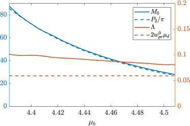
Figure 8: Plot of the ODE parameters $\Lambda$ and $M_{0}$ that best match the PDE trajectories with zero initial velocity. Same parameters as in Fig. 5. The blue dashed line corresponds to the estimate of the parameter $M_{0}$ from Ref. Ruban (2022) and the red dashed line shows the known zero-bright-mass frequency $\Lambda\approx 2\omega_{\rm pr}^{0}\mu_{d}$ (see text for details).

To compare the ODE reduction with the full GP dynamics in the stable regime of Fig. 5 we also depicted therein the value for $\dot{\theta}$ from the ODE model overlaid to demonstrate the frequency matching between the PDE and ODE models. This matching is done according to the following procedure. For a given flowering trajectory in the PDE model within appropriate parameter regimes, to obtain the corresponding ODE parameters we first identify those eigenvalues where the Krein signature bifurcates from zero to positive and negative values. The eigenvalues in Fig. 5 are color coded using (blue, black, red) points when the Krein sign is (negative, zero, positive). In particular, for a given $\mu_{b}$ value, we use the upper branch of the bifurcated eigenvalues to obtain the value $\dot{\theta}={\rm Im}(\nu)$. Then, by Eq. (18) we write the corresponding ODE $\Lambda$ parameter as:

$$\Lambda=2[\rho(r_{0})\dot{\theta}-M_{0}\dot{\theta}^{2}].$$ (26)

Having obtained $\Lambda$ as a function of $M_{0}$, a standard minimization procedure is then used to determine the initial VB ODE velocity and the $M_{0}$ value that best fit (in the least-squared sense) the ODE trajectory to the PDE trajectory. As can be seen in Fig. 5 (see cyan curves), this fitting procedure allows to accurately obtain the entire lower branch of the PDE bifurcating eigenvalues from the ODE frequencies of Eq. (19) as well as the critical point of the Hamiltonian Hopf bifurcation. This very good agreement lends strong credibility to our ODE reduction picture of the VB structure, i.e., Eqs. (10).

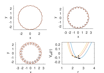
Figure 9: VB trajectories for $g_{12}=1.6$, $M=0.01$, $\mu_{d}=4.25$, and $\mu_{b}=4.56$. The VB is seeded at $x_{0}=2.5$ corresponding to a local chemical potential $\mu_{x_{0}}\approx 4.22$. To match the ODE trajectories we use $M_{0}\approx 18.9$. The top-left panel shows the resulting trajectory with initial velocities $k_{y}=0$ in the PDE (blue curve) and $\dot{y}(0)\approx 0.01$ in the ODE (red curve) with a resulting angular momentum of $\ell\approx 8.9$. For this value of $\ell$, the effective potential $V_{\rm eff}(r)$ in Eq. (16) is plotted in the bottom-right panel (blue). Three black dots are plotted on $V_{\rm eff}(r)$ corresponding to its minimum and the minimum and maximum radii of the trajectory. From these values we have an effective flower energy of $\Delta E\approx 0.002$ according to Eq. (28). Parameters are the same in the top-right panel except with initial velocities $k_{y}=0.1$ in the PDE and $\dot{y}(0)\approx 0.06$ in the ODE, with $\ell\approx 8.92$ giving the effective potential in the bottom-right panel (red) with $\Delta E\approx 0.01$. Similarly, the bottom-left panel corresponds to $k_{y}=0.15$ in the PDE and $\dot{y}(0)\approx 0.08$ in the ODE, while $\ell\approx 8.93$ giving the effective potential in the bottom-right panel (yellow) with $\Delta E\approx 0.03$. The thin black circles in the trajectory plots correspond to the circular orbits at the minima of the effective potentials.

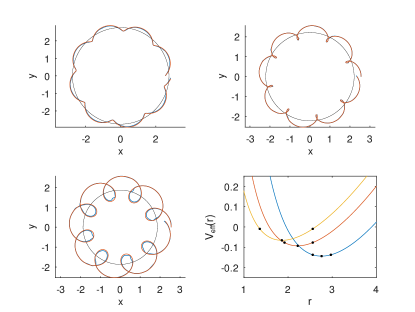
Figure 10: Similar to Fig. 9 with the same parameters except here $\mu_{b}\approx 4.47$, $M=0.02$, and $M_{0}\approx 37.0$. The top left panel has initial velocities $k_{y}=0$ in the PDE, and $\dot{y}(0)\approx 0.01$ in the ODE, $\ell\approx 8.9$, and $\Delta E\approx 0.006$. For this $\ell$, $V_{\rm eff}(r)$ is in the bottom right panel (blue). For the top right panel $k_{y}=0.1$ in the PDE, $\dot{y}(0)\approx 0.06$ in the ODE, with $\ell\approx 8.95$ to give the effective potential in the bottom right panel (red) with $\Delta E\approx 0.016$. Similarly in the bottom left panel $k_{y}=0.15$ in the PDE, $\dot{y}(0)\approx 0.08$ in the ODE, $\ell\approx 8.97$ and the corresponding effective potential is in the bottom right (yellow) with $\Delta E\approx 0.056$. Once again the thin black circles in the trajectory plots represent the circular orbits at the minima of the effective potentials.

Figure 8 depicts the corresponding ODE parameters across a range of $\mu_{b}$ values to the right of the Hamiltonian Hopf bifurcation point. The blue dashed line $P_{2}/\pi$ depicts the estimate for our ODE parameter $M_{0}$ according to Ref. Ruban (2022) [note their $(\tilde{M},M_{br})$ corresponds to our $(M_{0},P_{2})$ respectively as their Eq. (29) agrees with our Eq. (10); see also their Eq. (24) giving $M_{0}=M_{br}/\pi=P_{2}/\pi$]. The match of the relevant curves in Figure 8 is very good, revealing only a slight relative discrepancy of no more than $3.5\%$ for the estimate of $M_{0}$. On the other hand, the red dashed line corresponds to the precessional frequency of a vortex in the absence of the bright component given by $\Lambda=2\omega_{\rm pr}^{0}\mu_{d}$ obtained from Ref. Middelkamp et al. (2010) as follows. Taking our Eq. (10) with $M_{0}=0$ near the origin we obtain

$$\mu_{d}\dot{x} = -\frac{\Lambda}{2}y$$

(27)

$$\mu_{d}\dot{y} = \frac{\Lambda}{2}x.$$

Comparing this reduced system to Eqs. (3) and (4) of Ref. Middelkamp et al. (2010) gives $\Lambda=2w_{\rm pr}^{0}\mu_{d}\equiv\Omega^{2}\ln(8.88\mu_{d}/\Omega)$. The relatively large discrepancy between $\Lambda$ and the theoretical estimate may stem from the fact that the latter, rather than being a true estimate for the precessional frequency of the (massive) VB, it is just the precessional frequency corresponding to a vortex in the absence of the bright component. Note that, for this region of parameters (see Fig. 2), as $\mu_{b}$ increases the mass of the bright component decreases and thus, correspondingly, the $\Lambda$ curve progressively approaches the (red dashed) $\Lambda=2\omega_{pr}^{0}\mu_{d}$ non-filled vortex benchmark.

Direct comparisons between the PDE and ODE orbits are presented in Figs. 9 and 10 where the blue and red curves correspond to the PDE and ODE orbits respectively (the black circle corresponds to the circular orbit at the effective potential minimum; see below). The different cases in each figure are shown for a fixed value of $g_{12}$ and a fixed mass ratio $M$ for various initial velocities. For each trajectory, the angular momentum $\ell$ is obtained according to Eq. (12) and we compute the effective energy of the flower defined as:

$$\Delta E=V_{\rm eff}(r_{\rm max})-{\rm min}\{V_{\rm eff}\},$$ (28)

where $r_{\rm max}$ is the maximum radius (distance to the origin) attained by the orbit. In the bottom-right panels of Figs. 9 and 10 we also depict the ODE effective potential $V_{\rm eff}(r)$ according to Eq. (16). The corresponding overlaid black dots represent the minimum and extremal values of $V_{\rm eff}(r)$ attained through the flowering motion. For guidance we also overlay (see corresponding black circles), on top of the flowering trajectories, the circular orbits corresponding to the effective potential minima. Note that larger values of $\Delta E$ correspond to trajectories with bigger petals. It is also worth mentioning that, as it can be noticed from the values reported in Fig. 9, the initial velocities for the PDE ($k_{y}$) are larger than the fitted initial ODE velocities ($\dot{y}$). This apparent discrepancy is due to the fact that the VB initialization in the PDE is not perfect as we are just boosting the bright component with a velocity $k_{y}$ while we are not adjusting the velocity of the dark component. Therefore, part of the initial energy imparted to the VB in the PDE case is lost to background radiation while the bright hump accelerates the vortex in the dark component. As a result, the effective velocity that the VB acquires, after the initial radiation is emitted, is actually slightly smaller than $k_{y}$. Finding a better initialization procedure for the VB in the PDE model is an intriguing topic for further consideration. The associated difficulty is intimately connected to the “dual character” of the VB. On the one hand, it behaves as a vortical particle (for which at the one-component level, effective equations involve first-order ODEs and an initialization based purely on position), while it also behaves as a Newtonian particle with (bright-induced) mass, thus necessitating an initialization bearing both position and momentum information.

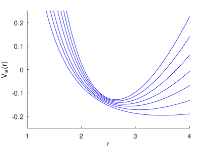
Figure 11: Effective potential $V_{\rm eff}(r)$ as the bright chemical potential $\mu_{b}$ is varied while all other parameters are the same as in Fig. 8. The different curves correspond to the values $\mu_{b}\approx 4.4,4.42,4.44,4.46,4.48,4.5,4.52$ where the shallower (steeper) effective potentials correspond to smaller (larger) values of $\mu_{b}$.

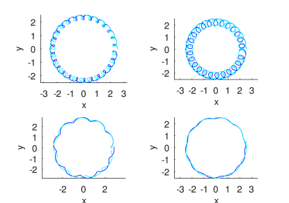
Figure 12: A comparison between flowering trajectories of the ODE system (dark blue) in Eqs. (10) and its corresponding linearization (cyan) as per Eqs. (LABEL:eq:estRTheta) and (LABEL:eq:omegaA). The top panels show the trajectories with $M_{0}\approx 17.95$, $\Lambda\approx 0.07$, and $\Omega=0.1$. In the top-left panel the initial velocity is $\dot{y}(0)=0.06$ giving an angular momentum $\ell\approx 8.93$, effective potential minimum at $r_{0}\approx 2.35$, effective energy $\Delta E\approx 0.01$, and the linearized prediction of $A_{0}\approx 0.1$, $R\approx 0.18$, and $(\omega_{r},\omega_{\rm pr})\approx(0.21,0.01)$. In the top-right panel the initial velocity is $\dot{y}(0)=0.08$ giving $\ell\approx 8.94$, $r_{0}\approx 2.22$, and $\Delta E\approx 0.04$ with linear predicted values $A_{0}\approx 0.17$, $R\approx 0.31$, and $(\omega_{r},\omega_{\rm pr})\approx(0.21,0.01)$. The bottom panels correspond to $M_{0}\approx 36.05$, $\Lambda\approx 0.08$, $\Omega=0.1$, and $(\omega_{r},\omega_{\rm pr})\approx(0.09,0.01)$. The bottom-left panel corresponds to $\dot{y}(0)=0.01$, $\ell\approx 8.9$, $r_{0}\approx 2.7$, $\Delta E\approx 0.004$, $A_{0}\approx-0.08$, and $R\approx 0.15$. The bottom-right panel corresponds to $\dot{y}(0)=0.03$, $\ell\approx 8.93$, $r_{0}\approx 2.49$, $\Delta E\approx 0.02$, $A_{0}\approx 0.04$, and $R\approx 0.07$.

Figure 11 sketches several plots of the effective potential $V_{\rm eff}(r)$ as the bright chemical potential $\mu_{b}$ is varied while all other parameters are fixed. Since larger $\mu_{b}$-values correspond to smaller mass ratios $M$, the resulting effective potentials are steeper. Here, we are capitalizing on the accuracy of our ODE-PDE comparison to infer the dynamical consequences of parametric variation at the PDE level, based on the ODE understanding. As a consequence, smaller bright masses will tend to produce flowering with smaller petals as a steeper potential means a larger initial energy (initial kick) in order to produce the same petal sizes. We should also point out that higher $g_{12}$ values result in flowering with a smaller frequency. Finally, Fig. 12 depicts several examples of flowering in the ODE and its corresponding linearized estimations as per Eqs. (LABEL:eq:estRTheta) and (LABEL:eq:omegaA). Note that the linearized equations are able to capture well the main shape and petal size of the flowering motion even modestly away from the linear regime. This suggests that Eqs. (LABEL:eq:estRTheta) and (LABEL:eq:omegaA) can be used as simple approximate analytical descriptors of the VB dynamics over a wide parametric range.

IV Summary and outlook

In the present work we have explored the topic of the dynamics of VB solitary waves deep within the immiscible regime. Our motivation in revisiting this subject stemmed from the renewed experimental ability to monitor such systems which creates the potential for connecting a particle-based understanding with a detailed analysis of the full PDE model. In that vein, we explored equilibrium solutions in this deeply immiscible regime (while some of the earlier studies of the present authors had confined themselves to regimes close to, e.g., hyperfine states of ⁸⁷Rb where the $g_{ij}$ coefficients are nearly equal Law et al. (2010)). In probing the excitations around the VB equilibrium state, we found the possibility of two frequencies of precession. One of these represents the frequency of precession that is well-familiar from a single-component vortex in a trap. The second frequency can be associated with the oscillation of the VB structure inside an effective radial potential (along the radial direction). The combination of these two frequencies gives rise to the potential for epicyclic motion, which, under suitable conditions discussed herein, can lead to “flowering”, i.e., to flower-like curves of the dynamics of the VB pattern. This intriguing feature, while observed and discussed previously Richaud et al. (2021); Ruban (2022) is here intimately connected between the ODE and PDE dynamics (both at the level of linearization and at that of fully nonlinear dynamical evolution). Our analysis enables both a reasonable approximate analytical description of the relevant motion and key byproducts thereof, such as the critical oscillation amplitude leading to flowering as a (simple) function of the precessional and radial oscillation frequencies. Among the additional intriguing features identified herein, we highlight the (oscillatory) instability of the VB structure when the relevant two frequencies collide. The result of the corresponding dynamics was found to be particularly unusual, in our experience of such systems. Indeed, as the VB embarks on a growing spiral oscillation, it becomes a patch of vorticity that gets elongated and eventually breaks into smaller patches carrying multiple localized phase jumps inside an extended region of vanishing density (in the so-called dark component) in a way reminiscent of persistent currents Wright et al. (2013).

While we considered a number of diagnostics (such as angular momentum-based ones) and visualizations (such as the 3D isocontours of vorticity) of this phenomenon, clearly it merits further study. An additional natural theme of study is to incorporate the (two or more) VB interactions to the model systematically developed herein, so as to examine the potential of formation of lattices (crystals) of such patterns. Understanding the modes of such crystals, their potential instabilities and dynamics promises to be an interesting avenue for the future. Furthermore, the states of interest can be generalized to three spatial dimensions where the natural analogue is the vortex-ring-bright (filled core) solitary wave Ruban et al. (2022); of course, vortex-line-bright structures exist too Charalampidis et al. (2016). A systematic particle-based understanding of such 3D settings is a natural generalization of the considerations provided herein. Relevant studies are currently in progress and will be reported in future publications.