Order parameters and phase transitions of continual learning in deep neural networks

Abstract

Continual learning (CL) enables animals to learn new tasks without erasing prior knowledge. CL in artificial neural networks (NNs) is challenging due to catastrophic forgetting, where new learning degrades performance on older tasks. While various techniques exist to mitigate forgetting, theoretical insights into when and why CL fails in NNs are lacking. Here, we present a statistical-mechanics theory of CL in deep, wide NNs, which characterizes the network’s input-output mapping as it learns a sequence of tasks. It gives rise to order parameters (OPs) that capture how task relations and network architecture influence forgetting and knowledge transfer, as verified by numerical evaluations. We found that the input and rule similarity between tasks have different effects on CL performance. In addition, the theory predicts that increasing the network depth can effectively reduce overlap between tasks, thereby lowering forgetting. For networks with task-specific readouts, the theory identifies a phase transition where CL performance shifts dramatically as tasks become less similar, as measured by the OPs. Sufficiently low similarity leads to catastrophic anterograde interference, where the network retains old tasks perfectly but completely fails to generalize new learning. Our results delineate important factors affecting CL performance and suggest strategies for mitigating forgetting.

¹ Center for Brain Science, Harvard University, Cambridge, Massachusetts 02138, United States
² Program in Neuroscience, Harvard Medical School, Boston, Massachusetts 02115, United States
³ Biophysics Graduate Program, Harvard University, Cambridge, Massachusetts, 02138, United States
⁴ Edmond and Lily Safra Center for Brain Sciences, Hebrew University, Jerusalem 9190401, Israel
⁵ hsompolinsky@mcb.harvard.edu
* These authors contributed equally to this work.

1 Introduction

Continual learning (CL), the capability to acquire and refine knowledge and skills over time, is fundamental to how animals survive in a non-stationary world. As an animal learns and performs many tasks, CL allows it to leverage previous learning to help learn a new task as well as to retain the ability to perform old ones. In artificial neural networks (NN), the cornerstone of recent advances in artificial intelligence, developing such abilities has been challenging. NNs especially struggle with catastrophic forgetting, where learning a new task overwrites existing information and dramatically degrades performance on previously learned tasks [1, 2, 3, 4]. This problem is so prevalent and severe in machine learning (ML) that it has become one of the biggest challenges for developing human-level artificial general intelligence [5, 6, 7]. Despite also relying on NNs for computation, the brain clearly does not suffer from catastrophic forgetting to nearly the same extent. Not only does this offer an “existence proof” of successful CL in NNs [3, 7, 8], it also raises intriguing questions about mechanisms underlying CL in the brain. A wide range of possible underpinnings, ranging from memory reactivation [9], synaptic stabilization [10, 11], to representational drift [12], have been proposed. However, their specific contributions to CL in the brain are not well understood.

Engineering CL in ML and identifying its mechanisms in the brain both suffer from a lack of theoretical understanding of the problem in NNs. Recently, analytical insights have been gained in the case where the network is a shallow linear network [13, 14, 15, 16, 17] or equivalently so via the neural tangent kernel (NTK) approximation [18, 19]. However, this setting does not account for the role of feature changes in CL. Moreover, it does not allow for the common and important scenario of having multiple readouts dedicated to different tasks. Another line of research, focusing on NNs with task-dedicated readouts, studied networks with one hidden layer containing a few neurons [20, 21, 22], limiting its application in realistic settings where there are usually hundreds of hidden units in each layer. Furthermore, a majority of these works [13, 14, 16, 17, 22, 20, 21, 23] rely on specific assumptions about the task data, making it difficult to generalize their conclusions to general tasks. While some studies have introduced theory-motivated metrics to quantify CL-relevant task relations in arbitrary data [24, 18], whether and how they are related to actual CL performance is unclear.

In this work, we propose a Gibbs formulation of CL and use tools from statistical physics to develop a comprehensive theory of CL in deep NNs. Our theory exactly describes how the input-output mapping of the network evolves as it sequentially learns more tasks, with or without task-specific readouts. Critically, these results do not rely on data assumptions, allowing the analysis of CL in a broad range of tasks. The theory connects the degree of forgetting and transfer learning during CL to relations between tasks, the NN’s architecture, and hyper-parameters of the learning process. Analytical and numerical evaluations identify two scalar order parameters (OP) capturing input and rule similarity between tasks and their sometimes contrasting effects on CL outcomes. These OPs prove to be predictive of CL performance on a range of datasets for NNs with and without task-specific readouts. The analysis also reveals how network depth and width strongly modulate CL performance. Increasing depth can mitigate forgetting by reducing the overlap between tasks, as captured by the depth-dependent OPs. For networks with task-dedicated readouts, our analysis identifies three dramatically different CL regimes, determined by the OPs and the amount of training data available relative to network width. Sequentially learning dissimilar tasks can lead to “catastrophic anterograde interference”, where previous learning causes the NN to overfit the latest task. Together, our results provide a rigorous treatment of the rich phenomena of CL in deep NNs and distinguish critical factors in task relations and architecture choices that promote or hinder CL. Implications for understanding the neuroscience of CL are discussed.

2 A Gibbs Formulation of CL in Deep Neural Networks

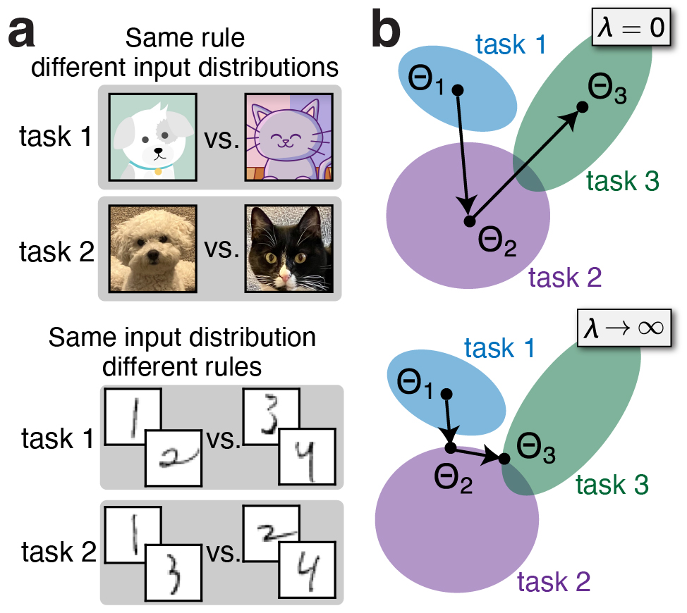
Figure 1: Schematics of CL and the Gibbs Formulation.
a The network learns a sequence of training datasets, each representing a task with an input distribution and a rule. Distributions and/or rules often differ between tasks, as illustrated by the schematics. The first sequence (top) consists of two tasks intuitively involving the same rule (cats vs. dogs) but different input distributions (cartoons or photos). The second sequence (bottom) involves the same input distribution (handwritten digits) but different rules (1, 2 vs. 3, 4 or 1, 3 vs. 2, 4).
b Weight-space schematics showing the Gibbs formulation of CL. Each dataset defines a space of solutions where the training loss is zero. The network learns the first task by sampling from its space of solutions. For subsequent tasks, the network assumes different solutions depending on the regularization strength ($\lambda$). At $\lambda=0$, learning of each task samples from its corresponding space of solutions independent of previous learning. At the other extreme of $\lambda\rightarrow\infty$, learning chooses the solution closest to the weights sampled while learning the previous task. These schematics assume $\beta\rightarrow\infty$.

We studied a task-based CL setting [25] where the network sequentially learns $T$ tasks with different input distributions and/or task rules (Fig. 1a), respectively represented by $T$ training datasets $D_{1},...,D_{T}$ of identical size. $D_{t}\equiv\left(\bm{X}_{t}\in\mathbb{R}^{P\times N_{0}},\bm{Y}_{t}\in\mathbb{R}^{P}\right)$, where $P$ is the number of examples per task and $N_{0}$ is the input dimensionality. Each row of $\bm{X}_{t}$, $\bm{x}_{t}^{\mu}$, is an input example with its corresponding label given by the $\mu$-th element of $\bm{Y}_{t}$, $y_{t}^{\mu}$. While learning task $t$, the network accesses $D_{t}$ but not the other datasets. We use “at time $t$” to refer to the state of the network after sequentially learning $D_{1}$ through $D_{t}$.

We first considered the simplest architecture: a multi-layer perceptron where all weights are shared across tasks (“single-head” CL [26, 27]). The network has $L$ fully-connected hidden layers, each containing $N$ nonlinear neurons, assumed to be ReLU for concreteness. The network load is denoted $\alpha\equiv P/N$. The input-output mapping of the network at time $t$ is given by

$$f_{t}\left(\bm{x}\right)\equiv\frac{1}{\sqrt{N}}\bm{a}_{t}\cdot\Phi(\mathcal{W}_{t},\bm{x}),$$ (1)

where $\bm{a}_{t}\in\mathbb{R}^{N}$ and $\mathcal{W}_{t}$ are the readout and hidden-layer weights at time $t$, respectively. $\Phi\left(\mathcal{W}_{t},\bm{x}\right)\in\mathbb{R}^{N}$ is the activation vector in the last hidden layer for input $\bm{x}\in\mathbb{R}^{N_{0}}$ (Methods), hereafter referred to as the representation of $\bm{x}$. The more complex “multi-head” CL scenario, where the network utilizes task-specific readouts, is introduced and studied later.

To mitigate forgetting, it is natural to constrain learning to favor small weight changes [11, 10, 6, 28]. We assume that learning $D_{t\geq 2}$ involves selecting the weights $\Theta_{t}\equiv\left\{\bm{a}_{t},\mathcal{W}_{t}\right\}$ according to a cost function

$$E\left(\Theta_{t}|\Theta_{t-1},D_{t}\right)\equiv\frac{1}{2}\sum_{\mu=1}^{P}\left(f_{t}\left(\bm{x}_{t}^{\mu}\right)-y_{t}^{\mu}\right)^{2}$$

$$+\frac{1}{2}\beta^{-1}\sigma^{-2}\left\|\Theta_{t}\right\|^{2}+\frac{1}{2}\beta^{-1}\lambda\left\|\Theta_{t}-\Theta_{t-1}\right\|^{2}.$$ (2)

The first term measures the error of $f_{t}$ on $D_{t}$. The second term acts as regularization that favors weights with small norm. The third term is the perturbation penalty that favors small weight changes relative to $\Theta_{t-1}$. $\beta>0$ denotes the inverse temperature, controlling how well $f_{t}$ interpolates $D_{t}$. $\sigma^{-2}>0$ and $\lambda\geq 0$ respectively scale the $L_{2}$ regularization and the perturbation penalty. This penalty is a simple variant of “regularization-based” methods for CL, where some variants [6, 28] apply different $\lambda$ to different weight elements and measure perturbation relative to all past weights. Our choice of the specific penalty form is motivated by its simplicity as well as recent empirical results suggesting that it can match the performance of more sophisticated variants [29]. The cost function for learning $D_{1}$, $E\left(\Theta_{1}|D_{1}\right)$, has the same form but without the penalty.

To make the problem amenable to analytical tools from statistical physics, we studied the equilibrium Gibbs distribution of $\Theta_{t}$ conditioned on $\Theta_{t-1}$, $P\left(\Theta_{t}|\Theta_{t-1},D_{t}\right)\equiv Z\left(\Theta_{t-1},D_{t}\right)^{-1}\exp\left(-\beta E\left(\Theta_{t}|\Theta_{t-1},D_{t}\right)\right)$, where $Z\left(\Theta_{t-1},D_{t}\right)$ is the normalization factor. This distribution defines a Markovian transition from $\Theta_{t-1}$ to $\Theta_{t}$, controlled by $D_{t}$. Multiplying all such distributions for $t\geq 2$ and the posterior of learning one task $P\left(\Theta_{1}|D_{1}\right)\equiv Z(D_{1})^{-1}\exp\left(-\beta E\left(\Theta_{1}|D_{1}\right)\right)$ yields a joint posterior over $\Theta_{1},...,\Theta_{T}$ [30, 16, 17],

$$P\left(\Theta_{1},...,\Theta_{T}|D_{1},...,D_{T}\right)=P\left(\Theta_{1}|D_{1}\right)\left[\prod_{t=2}^{T}Z\left(\Theta_{t-1},D_{t}\right)\right]^{-1}\exp\left(-\sum_{t=2}^{T}\beta E\left(\Theta_{t}|\Theta_{t-1},D_{t}\right)\right).$$ (3)

Eq. 3 fully describes how the network evolves during CL, from which various statistics can be calculated, including the marginals $P\left(\Theta_{t}|D_{1},...,D_{t}\right)$. We focus on over-parameterized NNs [31] in the $\beta\rightarrow\infty$ limit. In this case, there is usually a large space of $\Theta_{t}$ that perfectly interpolates the dataset $D_{t}$ as it comes (Fig. 1b). At $\lambda=0$, there is no coupling between weights from different times, and the network has no memory of previous tasks. On the other hand, at $\lambda\rightarrow\infty$, the network makes the minimum perturbation to weights necessary to interpolate $D_{t}$ [32]. This Gibbs formulation of CL allows us to characterize the distribution over the entire solution space after learning each task. While previous theoretical works on CL in wide DNNs [18, 24] assume linearization of the dynamics around initialization in the NTK regime [19], our Gibbs formulation does not rely on any assumptions on the learning dynamics. Interestingly, we recover a NTK-like theory of CL in the single-head scenario when $\lambda\rightarrow\infty$. However, we stress that the theoretical analysis in this work extends far beyond the NTK results, and is applicable in more realistic settings, in particular when $\lambda$ is finite, or when the number of training examples $P$ scales linearly with network width $N$, both resulting in substantial feature changes during CL.

Performance of the network on some dataset $D=\left(\bm{X},\bm{Y}\right)$ at time $t$ is measured by averaging the normalized mean-squared-error (MSE) loss,

$$\mathcal{L}(f_{t},D)\equiv\sum_{\mu}\left(f_{t}\left(\bm{x}^{\mu}\right)-y^{\mu}\right)^{2}/\left\|\bm{Y}\right\|^{2},$$ (4)

over the posterior of $\Theta_{t}$, denoted $\langle\mathcal{L}(f_{t},D)\rangle$. For the network that has learned $t$ tasks, we measure its forgetting of the training dataset of the $t^{\prime}$-th task ($t^{\prime}\leq t$) by computing $\mathcal{\langle L}(f_{t},D_{t^{\prime}})\rangle$, denoted $F_{t,t^{\prime}}$ for brevity. $F_{t,t}=0$ for all $t$ due to the $\beta\rightarrow\infty$ limit. We also evaluate its generalization of the $t^{\prime}$-th task by computing its performance on a test set $D_{t^{\prime}}^{test},$ $\mathcal{\langle L}\left(f_{t},D_{t^{\prime}}^{test}\right)\rangle$, denoted $G_{t,t^{\prime}}$. Analytically computing $\langle\mathcal{L}(f_{t},D)\rangle$ for an arbitrary $D$ requires the mean and variance of $f_{t}$. Using statistical-mechanics techniques, we developed a theory that provides exact expressions for them in terms of the $t$ tasks the network has already learned and hyperparameters such as $\lambda$ and $\sigma^{2}$. We then studied the theoretical expressions analytically and numerically to gain insights into important aspects of CL such as forgetting and knowledge transfer.

3 Networks Using a Readout Shared Across Tasks

3.1 Contrasting Impacts of Input and Rule Similarity on Forgetting in a Student-Teacher Setting

A major goal of CL research is to understand how relations between tasks affect CL performance. Our theory of single-head CL, exact in the infinite-width limit of $N\rightarrow\infty,\alpha\rightarrow 0$, allows analytical evaluations of $F_{t,t^{\prime}}$ and $G_{t,t^{\prime}}$ for arbitrarily long task sequences (Methods). Numerical analysis of the resultant expressions suggests that performance mainly depends on similarity between inputs of different tasks and between the tasks’ input-output rules. To analyze their respective effects, we first studied a student-teacher setting (Methods) with parameterized task relations (Fig. 2a). Each task consists of random inputs and labels generated by a “teacher” network. $\rho_{input}\in[0,1]$ controls input similarity: at $\rho_{input}=0$, inputs from different tasks have no correlation; at $\rho_{input}=1$, all tasks use the same inputs. Correlation between weights of different teachers is similarly controlled by $\rho_{teacher}\in[0,1].$ To simplify the analysis, we assume a small $\sigma^{2}$ where the variance of $f_{t}$ is small and $\left\langle\mathcal{L}\left(f_{t},D\right)\right\rangle\approx\mathcal{L}\left(\left\langle f_{t}\right\rangle,D\right).$ Finally, for now we assume $\lambda\rightarrow\infty$ and $L=1$, visiting these issues later on.

We first analyzed short-term forgetting, defined as forgetting on task 1 after learning one other task ($F_{2,1}$). Here, input and teacher similarity have opposing effects on forgetting. With increasing $\rho_{input}$, forgetting worsens (Fig. 2b). Under a given $\rho_{teacher}<1$, forgetting reaches its worst at $\rho_{input}=1,$ where $\bm{X}_{1}=\bm{X}_{2}$. On the other hand, forgetting worsens with decreasing $\rho_{teacher}$ (Fig. 2c), as the input-output mapping needed to fit $D_{1}$ increasingly conflicts with that for $D_{2}$. We next analyzed CL of a long sequence of tasks, which we term long-term forgetting. Forgetting of the first task ($F_{t,1}$) increases over time approximately as an exponential relaxation process (Methods), $F_{t,1}\approx F_{max}\left(1-e^{-(t-1)/\tau_{F}}\right)$ (Fig. 2d). We thus quantify long-term forgetting by its time constant $\tau_{F}$ and maximum $F_{max}$ – forgetting is worse with smaller $\tau_{F}$ and/or larger $F_{max}$. We found that $\tau_{F}$ is mainly determined by $\rho_{input}$ (Fig. 2e), with higher $\rho_{input}$ leading to faster forgetting (smaller $\tau_{F}$). On the other hand, $F_{max}$ is mainly determined by $\rho_{teacher}$, with higher $\rho_{teacher}$ leading to less maximum forgetting (smaller $F_{max}$; Fig. 2f). All together, for both short-term and long-term forgetting, forgetting is aggravated by higher input similarity and lower rule similarity.

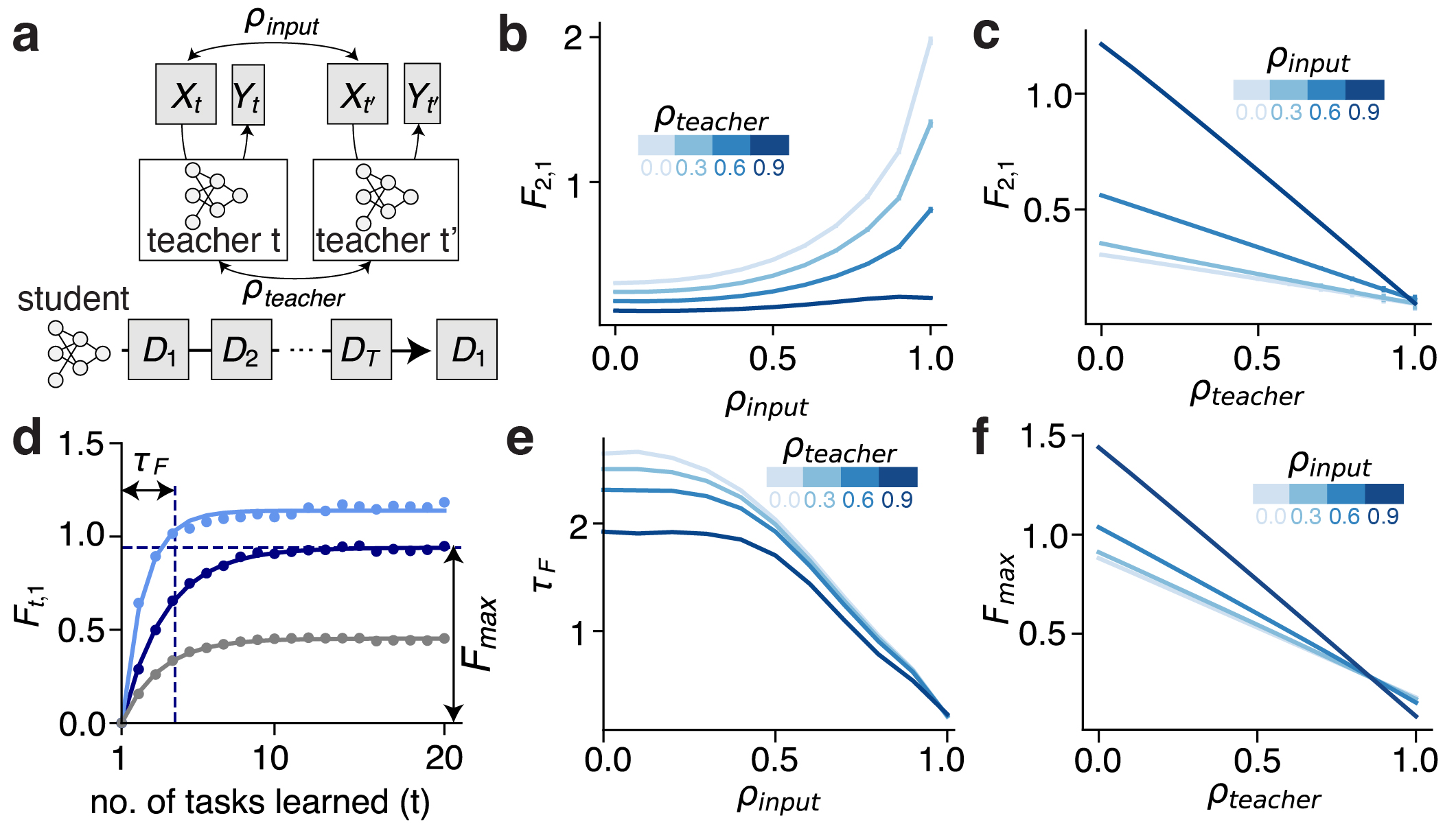
Figure 2: Effects of Input and Rule Similarity on Forgetting in a Student-Teacher Setting.
a Schematics of the generative process of the student-teacher tasks. Each task has random inputs and corresponding labels generated by a teacher network. The input similarity parameter ($\rho_{input}$) controls the correlation between inputs in different tasks; the teacher similarity parameter ($\rho_{teacher}$) controls the correlation between weights of different teacher networks. The student network learns the tasks sequentially and is evaluated on $D_{1}$ to measure forgetting.
b Forgetting on task 1 at time 2 ($F_{2,1}$) increases with $\rho_{input}$ for different fixed levels of $\rho_{teacher}$.
c $F_{2,1}$ decreases with $\rho_{teacher}$ for different fixed levels of $\rho_{input}$.
d Long-term forgetting is quantified by fitting an exponential relaxation process characterized by its time constant ($\tau_{F}$) and maximum ($F_{max}$). Each color indicates a different combination of $\rho_{input},\rho_{teacher}$ (dark blue: $0.1,0.1$; light blue: $0.1$,$0.7$; gray: $0.7,0.1$). Dots are actual forgetting; curves are fits.
e For each fixed level of $\rho_{teacher}$, $\tau_{F}$ decreases (faster forgetting) with $\rho_{input}$. Smaller $\tau_{F}$ indicates worse forgetting.
f For each fixed level of $\rho_{input}$, $F_{max}$ decreases (less maximum forgetting) with $\rho_{teacher}$. Larger $F_{max}$ indicates worse forgetting.
All $F_{t,1}$ have been numerically averaged over random seeds used for generating data. Error bars in b, c, d show standard error over 100 seeds.

3.2 Capturing Task Relations in General Datasets with CL Order Parameters

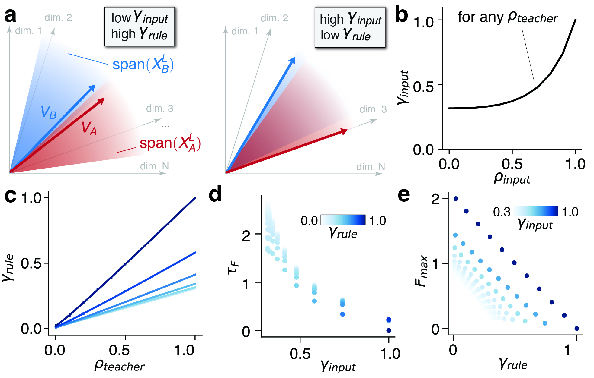
Figure 3: OPs of CL.
a Schematics illustrating the OPs of CL. Inside the $N$-dimensional space, representation vectors of inputs from each task ($\bm{X}_{A}^{L}$ or $\bm{X}_{B}^{L}$) span a P-dimensional linear subspace. Inside each subspace, the rule vector ($\bm{V}_{A}$ or $\bm{V}_{B}$) encodes the learned input-output rule of this task. The input overlap OP ($\gamma_{input}$, Eq. 5) measures the similarity between two subspaces, while the rule congruency OP ($\gamma_{rule}$, Eq. 6) measures the similarity between the rule vectors.
b Measured $\gamma_{input}$ as a function of $\rho_{input}$ in the student-teacher setting. $\gamma_{input}$ only depends on task inputs and thus is not affected by $\rho_{teacher}$ by definition.
c Measured $\gamma_{rule}$ as a function of $\rho_{teacher}$ in the same tasks as b. Each curve corresponds to a different fixed level of $\rho_{input}$.
d The time constant of long-term forgetting ($\tau_{F}$) decreases with $\gamma_{input}$, and only weakly depends on $\gamma_{rule}$. Each dot corresponds to a different $\rho_{input}$, $\rho_{teacher}$ combination.
e The maximum of long-term forgetting ($F_{max}$) decreases with $\gamma_{rule}$ for each fixed level of $\gamma_{input}$, and increases with $\gamma_{input}$ for each fixed level of $\gamma_{rule}$. The effect of $\gamma_{rule}$ is stronger.
Error bars in b and c show standard error over 100 random seeds used for data generation.

Our analysis above relies on a setting with controllable input distributions and task rules. In real-world CL settings, however, the generative processes of tasks are often implicit. Although human intuition can be used to estimate relations between inputs and rules from different tasks (Fig. 1a), it may not predict how a specific NN would sequentially learn these tasks. Therefore, we next studied how the effects of task relations on forgetting of a given network can be quantified and predicted using metrics computed from data. We introduce two theory-motivated scalar order parameters (OP) of CL that respectively measure the input overlap and rule congruency between tasks. These OPs are defined using representations of task inputs in a network with the same architecture as the learner but with Gaussian random hidden-layer weights, $\mathcal{W}_{0}$ (Methods).

For each of a pair of tasks $\left\{\left(\bm{X}_{i},\bm{Y}_{i}\right)\right\}_{i\in\{A,B\}}$, denote the representations of its inputs $\bm{X}_{i}^{L}\in\mathbb{R}^{P\times N}$, where the $\mu$-th row is given by $\Phi\left(\mathcal{W}_{0},\bm{x}_{i}^{\mu}\right)$. In the $N$-dim space of representations, these vectors span a $P$-dimensional linear subspace, characterized by the projection matrix $\bm{P}_{i}\equiv\left(\bm{X}_{i}^{L}\right)^{T}\left[\bm{X}_{i}^{L}\left(\bm{X}_{i}^{L}\right)^{T}\right]^{-1}\bm{X}_{i}^{L}$. The input overlap between tasks $A$ and $B$ is then defined as

$$\gamma_{input}\equiv\frac{\text{Tr}\left(\bm{P}_{A}\bm{P}_{B}\right)}{\sqrt{\text{Tr}\left(\bm{P}_{A}\right)\text{Tr}\left(\bm{P}_{B}\right)}}\in[0,1],$$ (5)

which provides a measure of normalized overlap between two subspaces (Fig. 3a). $\gamma_{input}$ is maximized at $1$ when the two subspaces are identical and minimized at $0$ when they are non-overlapping.

To define the rule congruency OP, we introduce the mean readout vector if the network with random hidden-layer weights learns $\left(\bm{X}_{i},\bm{Y}_{i}\right)$ alone, given by $\bm{V}_{i}\equiv\left(\bm{X}_{i}^{L}\right)^{T}\left[\bm{X}_{i}^{L}\left(\bm{X}_{i}^{L}\right)^{T}\right]^{-1}\bm{Y}_{i}\in\mathbb{R}^{N}$, referred to as the rule vector. Rule congruency between tasks $A$ and $B$ is defined by the cosine similarity of their rule vectors (Fig. 3a)

$$\gamma_{rule}\equiv\frac{\bm{V}_{A}^{T}\bm{V}_{B}}{\left\|\bm{V}_{A}\right\|\left\|\bm{V}_{B}\right\|}\in[-1,1].$$ (6)

Two identical datasets would yield $\gamma_{rule}=1$ whereas two datasets with identical inputs but opposite labels would yield $\gamma_{rule}=-1$.

To illustrate characteristics of the OPs, we first computed them on student-teacher tasks as we systematically varied $\rho_{input}$ and $\rho_{teacher}$. By definition, $\gamma_{input}$ only depends on $\rho_{input}$ and not on $\rho_{teacher}$ (Fig. 3b). At $\rho_{input}=1$, the inputs are identical and $\gamma_{input}$ is maximized at $1$. On the other hand, $\gamma_{input}$ is non-zero at $\rho_{input}=0$, since two sets of uncorrelated random inputs with high probability still span overlapping subspaces in the representation space. Unlike $\gamma_{input}$, $\gamma_{rule}$ in general changes with both $\rho_{input}$ and $\rho_{teacher}$ (Fig. 3c). Its dependence on $\rho_{teacher}$ is intuitive – more similar teachers produce tasks with more congruent rules. Its dependence on $\rho_{input}$ reflects the important fact that, even when both tasks use the same teacher ($\rho_{teacher}=1$), the student network may still end up learning different rules when the input examples are different ($\rho_{input}<1$). These results also point to the general phenomenon where changing the input relations between two tasks usually affects both OPs, whereas changing the relation between their labeling rules affects $\gamma_{rule}$ alone.

For the student-teacher tasks, we found that measuring the two OPs is sufficient for qualitatively predicting the severity of forgetting across sequences with different task relations. For short-term forgetting, higher $\gamma_{input}$ and lower $\gamma_{rule}$ are associated with worse forgetting (Supplementary Note 4). In the long-term, $\tau_{F}$ is negatively correlated with $\gamma_{input}$ (Fig. 3d) and does not significantly depend on $\gamma_{rule}$. On the other hand, $F_{max}$ depends on both OPs (Fig. 3e), increasing with $\gamma_{input}$ and decreasing with $\gamma_{rule}$, although it is more sensitive to the latter. In summary, in both the short-term and long-term, high $\gamma_{input}$ and lower $\gamma_{rule}$ are associated with worse forgetting. Higher $\gamma_{input}$ predicts faster forgetting (lower $\tau_{F}$) and relatively weakly predicts higher maximum forgetting (higher $F_{max}$) whereas lower $\gamma_{rule}$ strongly predicts higher $F_{max}$.

3.3 Using Order Parameters to Predict Forgetting in Benchmark Sequences

To see how well $\gamma_{input}$ and $\gamma_{rule}$ capture the effects of task relations on CL performance over general data, we analyzed several benchmark task sequences. Following standard practices, we created each sequence by applying a generation protocol, specified below, to a multi-way classification dataset (“source datasets”): MNIST [33], EMNIST [34], Fashion-MNIST [35], or CIFAR-100 [36]. To generate long task sequences ($T\gg 2$) for the long-term forgetting analysis, we used the split protocol [28] and , where a higher “permutation ratio” corresponds to less similar inputs between tasks. To analyze anterograde transfer from one task to the next, we also devised a “label-flipping” protocol, which produces sequences of two tasks with inputs independently drawn from the same distribution but labelled using different rules – a higher “flipping ratio” corresponds to less similar rules. Further details and rationales are provided in Methods.

We first computed the OPs for the task sequences, aggregated over the specific source datasets used (Fig. 4a). Among permutation sequences, $\gamma_{input}$ decreases as the permutation ratio increases, as expected. This also leads to a sharp decrease of $\gamma_{rule}$, highlighting the input dependence of $\gamma_{rule}$. For label-flipping tasks, since changing the flipping ratio does not affect the inputs, it only alters $\gamma_{rule}$. Notably, $\gamma_{rule}$ drops below zero with a high flipping ratio.

To analyze long-term forgetting over split and permutation sequences, we again computed $F_{t,1}$ on sequences of length $T\sim O\left(10^{2}\right)$ and fitted them with exponential relaxation (Fig. 4b; Methods). Full-permutation sequences and split sequences exhibit similar OPs. As predicted, forgetting on these sequences has similar $\tau_{F}$ and $F_{max}$ (dark blue and green bars). Among permutation sequences, those generated with a higher permutation ratio are expected to have lower $\tau_{F}$, since the measured $\gamma_{input}$ is lower. In addition, they are anticipated to have higher $F_{max}$ – although lower $\gamma_{input}$ alone predicts lower $F_{max}$, tasks with stronger permutation also have substantially lower $\gamma_{rule}$, which increases $F_{max}$ with a stronger effect. Both predictions are consistent with our observations.

Having varied the OPs by adjusting task-generation procedures, we next studied the effects of the network depth ($L$). $L$, so far assumed to be 1, affects the OPs by modifying $\Phi(\mathcal{W}_{0},\bm{x})$. Across task sequences, increasing $L$ leads to a consistent reduction of both OPs towards $0$ (Fig. 4c, d), indicating that representations for different tasks become more separated in deeper networks. To analyze whether the depth-induced changes to the OPs are associated with different forgetting severity, we next computed $F_{t,1}$ for the same task sequences studied in Fig. 4b but assuming various $L$. Consistent with the notion that lower $\gamma_{input}$ predicts slower forgetting (higher $\tau_{F}$), $\tau_{F}$ across task sequences is increased as the network becomes deeper (Fig. 4e). Furthermore, the relation between $\tau_{F}$ and $\gamma_{input}$ appears conserved across task-sequence types and depth (Fig. 4f). On the other hand, the effect of depth on $F_{max}$ is more complex since it depends on both OPs. The picture is simpler for task sequences with $\gamma_{rule}\approx 0$ at $L=1$ (100% permutation and split sequences, see Fig. 4d). In their case, the only salient effect from increasing depth is the reduction of $\gamma_{input}$, which predicts a lower $F_{max}$, as confirmed by the analysis of $F_{t,1}$ (Fig. 4g). Thus, for these datasets, increasing depth brings both slower forgetting (higher $\tau_{F}$) and lower maximum (lower $F_{max}$). However, for sequences with high $\gamma_{rule}$ at $L=1$, the depth-induced reduction in $\gamma_{rule}$ could overcome benefits from reduced $\gamma_{input}$ on $F_{max}$ and result in slightly increased $F_{max}$ (Fig. 4g). In conclusion, the same tasks are represented less similarly (lower OPs) by deeper networks, resulting in significantly slower forgetting but sometimes higher maximum forgetting.

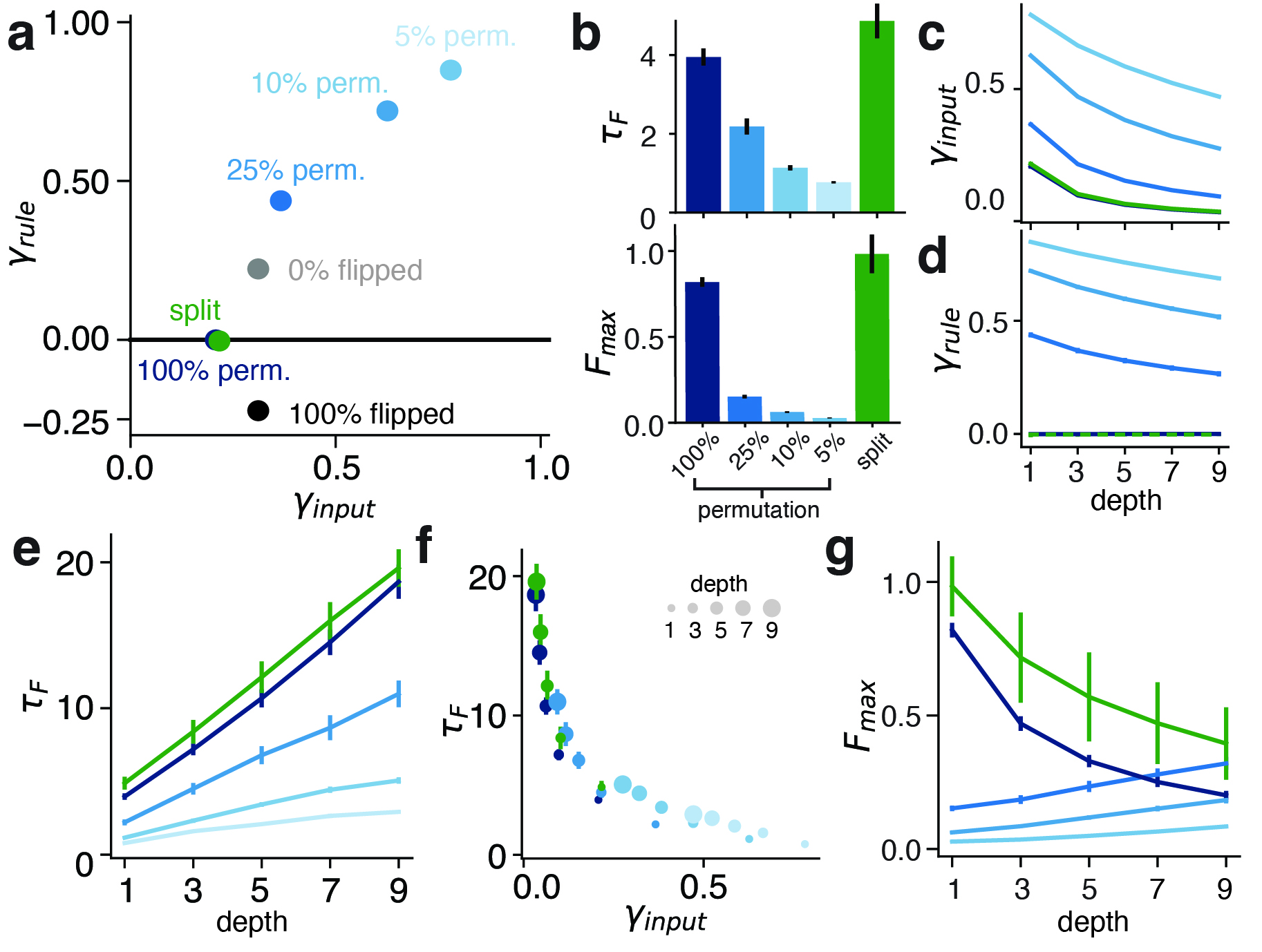
Figure 4: OPs of CL on Benchmark Task Sequences.
a 2D diagram showing input overlap ($\gamma_{input})$ and rule congruency ($\gamma_{rule}$) computed on different benchmark CL task sequences.
b Fitted exponential-relaxation parameters on long-term forgetting on permutation and split sequences.
c, d $\gamma_{input}$ and $\gamma_{rule}$ decrease towards zero with network depth ($L$) for all sequence types.
e The time constant of forgetting ($\tau_{F}$) increases with network depth (slower forgetting), as predicted by the decrease in $\gamma_{input}$ in c.
f The relation between $\tau_{F}$ and $\gamma_{input}$ across sequences and depths. Here, each dot corresponds to a combination of sequence type and the depth. Each sequence type has five dots corresponding to networks of depths 1, 3, 5, 7, and 9. Dots with smaller sizes represent shallower networks.
g Dependence of the maximum forgetting ($F_{max}$) on $L$.
Not all combinations of source datasets and protocols were studied (Methods). OPs are averaged over random seeds used for procedures during task generation as well as the source datasets used. Error bars in a-g, sometimes not visible, indicate standard error over different source datasets.

3.4 Task Relations and Anterograde CL

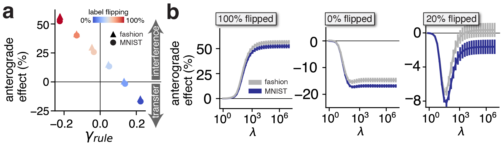
Figure 5: Anterograde Effects on Generalization.
a The anterograde effect, defined as $(G_{2,2}-G_{2}^{0})/G_{2}^{0}$ (see text), measures how learning task 1 affects the test loss on task 2. When the label-flipping ratio is 0%, the two datasets $D_{1},D_{2}$ contain images labelled with the exact same rule. $(G_{2,2}-G_{2}^{0})/G_{2}^{0}<0$, indicating knowledge transfer. As the label-flipping ratio increases, the underlying rules become more distinct. As a result, rule congruency ($\gamma_{rule}$) decreases and the anterograde effect changes from transfer to anterograde interference, where $(G_{2,2}-G_{2}^{0})/G_{2}^{0}>0$.
b The effect of perturbation penalty strength ($\lambda$) on the anterograde effect depends on rule congruency. For very incongruent (100% flipping) or very congruent (0% flipping) tasks, reducing $\lambda$ lessens interference or transfer, respectively. However, for tasks of intermediate congruency (e.g., 20% flipping), the anterograde effect is highly non-monotonic in $\lambda$ and optimized at a finite value.
Error bars show standard error over 50 random seeds used for task generation.

The analysis so far has focused on forgetting, where subsequent learning degrades performance on old tasks. However, in many important CL applications such as curriculum learning [37] and concept-drift adaptation [38], the emphasis is instead placed on how previous learning affects the network’s ability to learn and perform the latest task. To study this aspect, we quantified the anterograde effect of learning a previous task on the generalization performance of the second task with $(G_{2,2}-G_{2}^{0})/G_{2}^{0}$, where $G_{2,2}\equiv\left\langle\mathcal{L}\left(f_{2},D_{2}^{test}\right)\right\rangle$ and $G_{2}^{0}$ is the test loss on task 2 if the NN has learned it alone. A positive value indicates that prior learning increases the test loss and thus indicates anterograde interference; a negative value suggests knowledge transfer. We chose to focus on the generalization performance since the network always reaches zero training error on the second task after learning.

We hypothesized that a single-head network would struggle with anterograde interference more when the tasks contain conflicting rules. If true, the rule congruency OP, $\gamma_{rule}$, should predict the anterograde effect. To test this, we analyzed the relation between $\gamma_{rule}$ and $(G_{2,2}-G_{2}^{0})/G_{2}^{0}$ in label-flipping tasks by varying the flipping ratio, and uncovered a strong anti-correlation (Fig. 5a). These results indicate that single-head CL is prone to anterograde interference, whereas knowledge transfer only occurs at minimal levels of label flipping and thus relatively high rule congruency (see Discussion).

We next studied the perturbation-penalty parameter $\lambda$ (Eq. 2), so far assumed to be infinite to minimize forgetting. Since $\lambda=0$ completely removes dependence of $\Theta_{t}$ on $\Theta_{t-1}$, the network has no memory of previous learning (complete forgetting) and $G_{2,2}=G_{2}^{0}$ regardless of task relations. Adjusting $\lambda$ between zero and infinity provides a parametric way for controlling the anterograde effect. When task rules are strongly incongruent (100% flipping, Fig. 5b left) or congruent (0% flipping, Fig. 5b middle), reducing $\lambda$ lowers the magnitude of anterograde interference/transfer in a mostly monotonic manner. Interestingly, at intermediate levels of congruency (20% flipping, Fig. 5b right) tuning $\lambda$ can have a highly non-monotonic effect, demonstrating how a finite $\lambda$ can optimally balance leveraging transfer and mitigating interference.

4 Networks with Task-Dedicated Readouts

4.1 Setup of Multi-Head CL

In many CL settings, both in ML applications and naturalistic environments for animals, the learner is aware (through external cues or inference) of the identity of the current task being learned or performed. A simple method of incorporating such information into the NN, popular in ML [26, 27], is to use task-specific readouts (“multi-head” CL). When learning a new task, the NN modifies the hidden-layer weights and adds a new task-specific readout, leaving previous readouts untouched (Fig. 6 a). The network has $t$ different input-output mappings after learning $t$ tasks, given by

$$f_{t}^{\tau}({\bf x})\equiv\frac{1}{\sqrt{N}}\bm{a}_{\tau}\cdot\Phi\left(\mathcal{W}_{t},\bm{x}\right)\quad\tau=1,\cdots,t.$$ (7)

At time $t$, the network selects the mapping $f_{t}^{\tau}(\bm{x})$ to perform the $\tau$-th task. Since the readout weights $\left\{\bm{a}_{\tau}\right\}_{\tau=1,\cdots,t}$ are task-dedicated and the hidden-layer weights $\mathcal{W}_{t}$ are shared, only the changes in $\mathcal{W}_{t}$ need to be constrained in order to mitigate forgetting. Due to these differences from single-head CL, the Gibbs formulation of multi-head CL is given by Eq. 2 but with $f_{t}(\bm{x})$ replaced with $f_{t}^{t}(\bm{x})$ and the regularization term $\lVert\Theta_{t}-\Theta_{t-1}\rVert^{2}$ replaced with $\lVert\mathcal{W}_{t}-\mathcal{W}_{t-1}\rVert^{2}$.

The presence of task-specific parameters generally makes forgetting less severe than that in single-head CL [39]. Importantly, this architecture allows the network to perform conflicting tasks, which single-head networks struggle with, as shown in the previous section. In fact, if we consider multi-head networks at the same infinite-width limit ($N\rightarrow\infty,$ $\alpha\rightarrow 0$) where single-head networks were studied above, forgetting and anterograde effects (interference but also transfer) can be entirely avoided regardless of task relations, since the network can simply freeze its random hidden-layer weights and learn a separate readout for each task. However, this simple scheme breaks down in the more realistic cases where resources are limited and the network may have to modify the hidden-layer weights to solve each task. To study CL in this case, we switched to the thermodynamic limit, defined by $P,N\rightarrow\infty$ and $\alpha\sim\mathcal{O}(1)$ (Methods). The theory in this regime is more complex, hence we focused on the case of $T=2$ and $L=1$, although numerical results beyond these restrictions show similar qualitative behaviors (Supplementary Note 5.1). Furthermore, while in single-head CL we neglected the variance of $f_{t}$ and approximated $\left\langle\mathcal{L}(f,D)\right\rangle$ as $\mathcal{L}(\langle f\rangle,D)$, we do not make such approximation in multi-head CL as the variance could drive $\left\langle\mathcal{L}(f,D)\right\rangle$ to divergence, as shown in later sections. Our theory analytically provides the mean and variance of $f_{2}^{1}$, $f_{2}^{2}$ as a function of $D_{1}$ and $D_{2}$ (Methods). This allows evaluating forgetting of task 1 and generalization error on task 2 in multi-head CL, respectively given by $F_{2,1}=\left\langle\mathcal{L}\left(f_{2}^{1},D_{1}\right)\right\rangle$ and $G_{2,2}=\left\langle\mathcal{L}\left(f_{2}^{2},D_{2}^{test}\right)\right\rangle$.

4.2 Phase Transitions in CL Performance in the Student-Teacher Setting

We again began by using the student-teacher tasks to probe how task relations affect CL performance in the limit of $\lambda\rightarrow\infty$. In addition to varying $\rho_{input}$ and $\rho_{teacher}$ as in the single-head analysis, we also varied the load $\alpha$. We chose task sequences generated under three pairs of $\rho_{input},\rho_{teacher}$ as examples and computed $F_{2,1}$ and $G_{2,2}$ as $\alpha$ increases. We found that, regardless of task relations, $F_{2,1}$ is zero as long as $\alpha<1$, while $G_{2,2}$ diverges to infinity as $\alpha$ approaches $1$ (Fig. 6b). To understand the zero forgetting, we analyzed how network representations of task 1 inputs changed due to learning task 2, denoted $\Delta\Phi(\bm{X}_{1})\equiv\Phi(\mathcal{W}_{2},\bm{X}_{1})-\Phi(\mathcal{W}_{1},\bm{X}_{1})$, and found that it has zero norm as long as $\alpha<1$ (Supplementary Note 2.6.2). Such behaviors can be explained by the fact that when $\alpha<1$, learning the task-2 readout ($\bm{a}_{2}$) alone is sufficient to interpolate $D_{2}$, requiring no change to the hidden-layer weights ($\mathcal{W}$). Due to the strong perturbation penalty ($\lambda\rightarrow\infty$), $\mathcal{W}$ do not change, maintaining the network representations after learning task 1. This can also explain the divergence of $G_{2,2}$ as $\alpha\rightarrow 1$: learning $D_{2}$ by modifying $\bm{a}_{2}$ on top of the $N$-dimensional fixed representations is effectively a linear regression, the generalization error of which is well known to diverge as $P$ approaches $N$ [40]. For smaller $\alpha$, the zero $F_{2,1}$ and moderate $G_{2,2}$ demonstrate the advantage of using task-specific readouts. We term this regime of $\alpha<1$, where $F_{2,1}=0$ and $G_{2,2}$ is mostly finite, the “fixed representations” regime.

As $\alpha$ increases past 1, interpolating $D_{2}$ requires changing $\mathcal{W}$. Consequently, we expected that such changes would induce forgetting of task 1. Surprisingly, we found that there exists a critical load, $\alpha_{c}>1$, under which forgetting remains zero (Fig. 6c). Further analysis shows that while $\Delta\Phi(\bm{X}_{1})$ no longer has zero norm, it is confined within the null space of $\bm{a}_{1}$ and thus do not alter the output on task 1 (Supplementary Notes 2.6.2, 5). Although the absence of forgetting is desirable, this regime is accompanied by the network’s inability to generalize on the second task, despite reaching zero training error. In fact, $G_{2,2}$ diverges (Fig. 6d, bottom), indicating the surprising phenomenon we term “catastrophic anterograde interference”, where previous learning completely impedes generalization of new learning. We term this regime, where $F_{2,1}=0$, and $G_{2,2}\rightarrow\infty$, the “overfitting” regime. As $\alpha$ increases past $\alpha_{c}$, the network abruptly enters the “generalization” regime where $F_{2,1}>0$ and $G_{2,2}$ becomes finite. In this regime, $\Delta\Phi(\bm{X}_{1})$ is no longer confined to the null space of $\bm{a}_{1}$, inducing forgetting. The network partially forgets task 1, but learns to generalize on task 2.

Importantly, the boundary separating the two regimes ($\alpha_{c}$) depends on task relations. Each combination of $\rho_{input},\rho_{teacher}$ (Fig. 6c) is associated with a different $\alpha_{c}$. To fully understand such dependence, we analytically estimated $\alpha_{c}$ for a fixed level of $\rho_{input}$ and different $\rho_{teacher}$ (Fig. 6d; Supplementary Note 2.5) and for a fixed level of $\rho_{teacher}$ and different $\rho_{input}$ (Fig. 6e). Increasing $\alpha$ (as done in Fig. 6b, c) amounts to moving horizontally from left to right on such diagrams; the transition into generalization occurs when the horizontal line crosses the boundary. $\alpha_{c}$, jointly determined by $\rho_{input}$ and $\rho_{teacher}$, is small only when both $\rho_{input}$ and $\rho_{teacher}$ are high (Fig. 6f), indicating that both input and rule similarity need to be high for the overfitting regime to be small. These results also highlight the fact that, while both single-head and multi-head CL are strongly dependent on task relations, the nature of such dependencies can be drastically different.

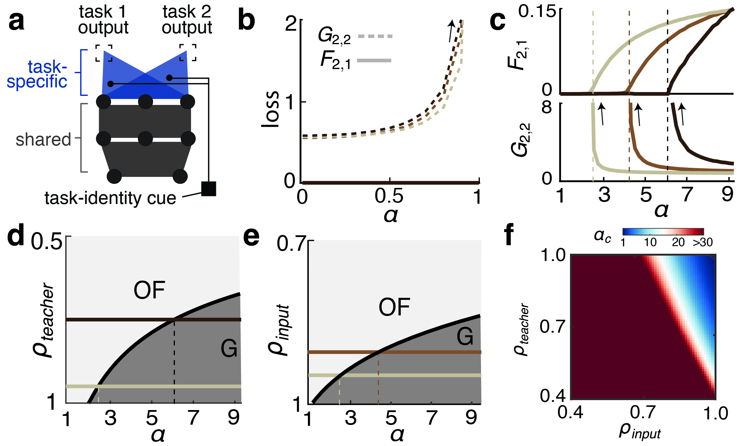
Figure 6: Multi-Head CL Exhibit Phase Transitions in the Student-Teacher Setting.
a Schematics of multi-head CL. Different tasks utilize the same shared hidden-layer weights but different task-specific readouts. The weight-perturbation penalty is only applied to the hidden-layer weights.
b Forgetting of task 1 ($F_{2,1}$) and the generalization error on task 2 ($G_{2,2}$) as a function of the network load ($\alpha$) for different $\rho_{input},\rho_{teacher}$ in the fixed-representations regime ($\alpha<1$). Black arrows indicate divergence towards infinity as $\alpha$ approaches 1. Curves of different colors correspond to tasks with different $\rho_{input},\rho_{teacher}$. light: 0.95, 0.95; medium: 0.9,0.95; dark: 0.95, 0.75.
c Same as b, but for $\alpha>1$. For each $\rho_{input},\rho_{teacher}$ combination, $F_{2,1}$ and $G_{2,2}$ exhibit abrupt changes as $\alpha$ crosses a critical load ($\alpha_{c}$, vertical dashed line). In the overfitting regime $(1<\alpha<\alpha_{c}$), $F_{2,1}$ is zero but $G_{2,2}$ diverges. In the generalization regime ($\alpha>\alpha_{c}$), both $F_{2,1}$ and $G_{2,2}$ can be moderate, finite, and nonzero.
d $\rho_{teacher}-\alpha$ phase diagram showing the overfitting (“OF”) and generalization (“G”) regimes ($\rho_{input}$ is fixed at 0.95). Higher $\rho_{teacher}$ and $\alpha$ lead to the generalization regime, and lower $\rho_{teacher}$ or $\alpha$ leads to the overfitting regime. The black curve marks the transition boundary. The horizontal lines mark the range of parameters shown in b, c.
e Same as d, but in $\rho_{input}-\alpha$ space with fixed $\rho_{teacher}$ at 0.95.
f $\alpha_{c}$ as a function of $\rho_{input}$ and $\rho_{teacher}$. $\alpha_{c}$ is higher for less similar (lower $\rho_{input}$ or $\rho_{teacher}$) tasks, meaning that the overfitting regime is larger and harder to avoid. Both $\rho_{input}$ and $\rho_{teacher}$ need to be high to have small $\alpha_{c}$.

4.3 CL Order Parameters Determine Phase Boundaries

Our analytical results suggest that the three phases are in fact general phenomena and not quirks of the student-teacher tasks. To verify, we selected two permuted MNIST sequences with different permutation ratios (Fig. 7a; Methods) and again computed $F_{2,1}$and $G_{2,2}$ as we varied $\alpha$. The analysis revealed the same three regimes as observed above: when $\alpha<1$, $F_{2,1}$ is zero and $G_{2,2}$ diverges as $\alpha\rightarrow 1$ (fixed representations); when $\alpha$ is between 1 and a critical load $\alpha_{c}$, $F_{2,1}$ remains zero while $G_{2,2}$ stays infinite (overfitting). Finally, at $\alpha>\alpha_{c}$, $F_{2,1}$ and $G_{2,2}$ are both finite (generalization). Repeating the same analysis with split MNIST sequences with different split ratios (Methods) further confirmed the generality of these regimes (Fig. 7b). Furthermore, these qualitative behaviors were reproduced in gradient-descent trained networks (Supplementary Note 5.1) as well as CL of longer task sequences (Supplementary Note 8).

Consistent with findings from student-teacher sequences, $\alpha_{c}$ is affected by changing the permutation/split ratio, which affects relations between tasks. We analytically estimated how $\alpha_{c}$ depends on these ratios (Methods), producing a phase diagram for each type of sequence (Fig. 7c, d). Importantly, we found that under some heuristic approximations, $\alpha_{c}$ is fully determined by the OPs $\gamma_{input}$ and $\gamma_{rule}$ for general task sequences, as defined in earlier sections (Fig. 7 e, f; Supplementary Note 2.5), suggesting that these two OPs capture the effects of task relations on CL performance in both single-head and multi-head scenarios. This finding allows us to study the effect of input/rule similarity on $\alpha_{c}$ in generality by computing it for different $\gamma_{input},\gamma_{rule}$ (Fig. 7g). This revealed a similar qualitative picture as Fig. 6g, where the overfitting regime is larger and requires a larger $\alpha$ to avoid when tasks have low input or rule similarity.

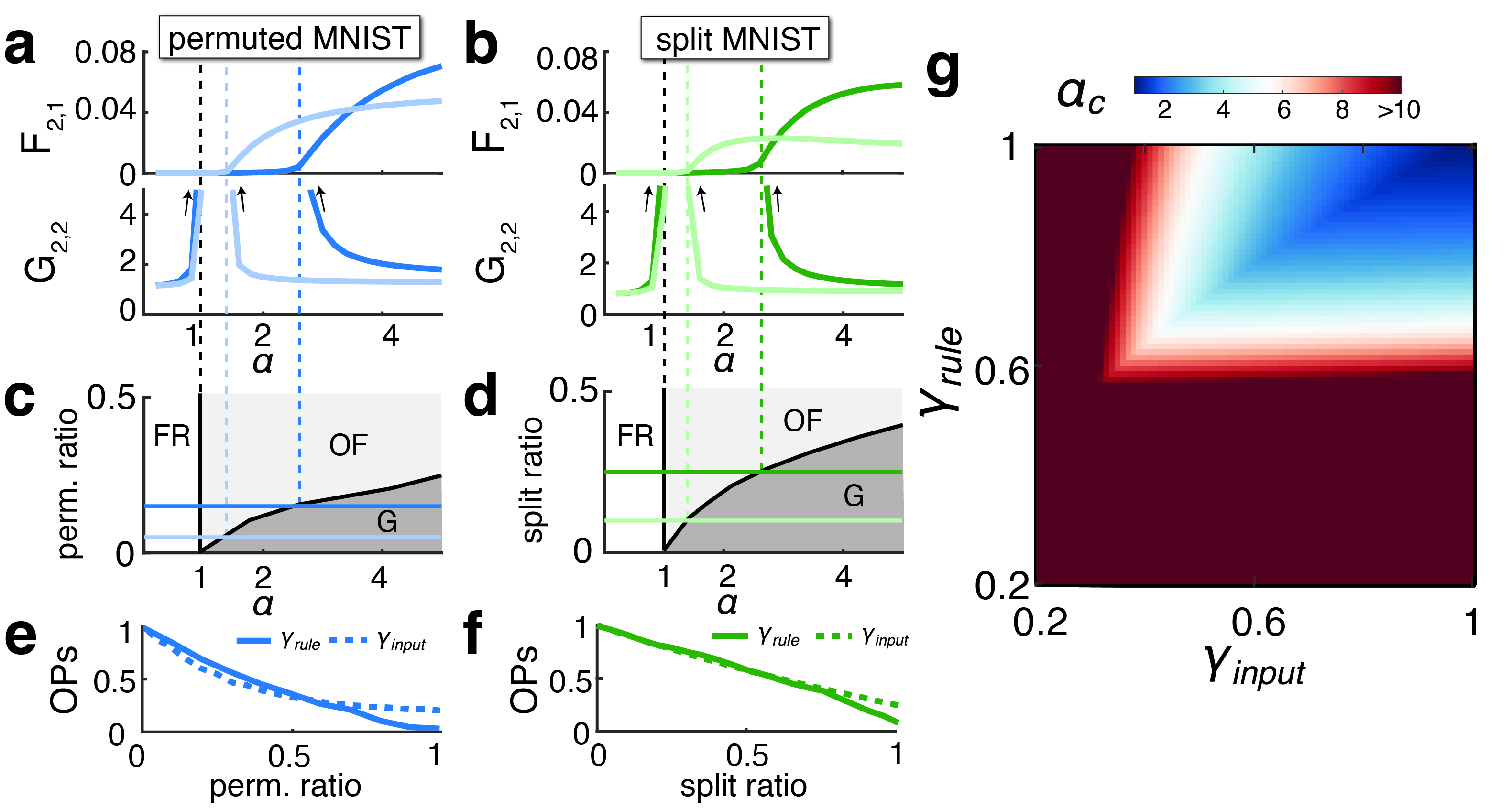
Figure 7: Transition Boundaries Predicted by the OPs of CL.
a Forgetting of task 1 ($F_{2,1}$) and the generalization error on task 2 ($G_{2,2}$) as a function of the network load ($\alpha$) for permuted MNIST sequences. Darker/lighter curves correspond to sequences with two permutation ratios (darker curve: 15%, lighter curve: 5%. See Methods). $F_{2,1}$ transitions from 0 to nonzero at the critical load ($\alpha_{c}$); correspondingly, $G_{2,2}$ starts to diverge at $\alpha=1$, and returns to a finite value at $\alpha_{c}$.
b Same as a, but for split MNIST sequences with two split ratios (darker curve: 25%, lighter curve: 15%. See Methods).
c Phase diagram of permuted MNIST in the permutation ratio-$\alpha$ space (truncated for readability) showing the three regimes: fixed representations (“FR”), overfitting (“OF”) and generalization (“G”). It reveals the same regimes as in Fig. 6. The horizontal lines mark the parameters plotted in a.
d Same as c, but showing the regimes in split ratio-$\alpha$ space for split MNIST sequences.
e, f Adjusting the permutation/split ratio affects both OPs, which in turn determine $\alpha_{c}$.
g $\alpha_{c}$ as a function of input overlap ($\gamma_{input}$) and rule congruency ($\gamma_{rule}$). Larger $\gamma_{input}$ and $\gamma_{rule}$ lead to smaller $\alpha_{c}$, indicating a smaller overfitting regime.

4.4 Balancing Memorization and New Learning with Finite $\lambda$

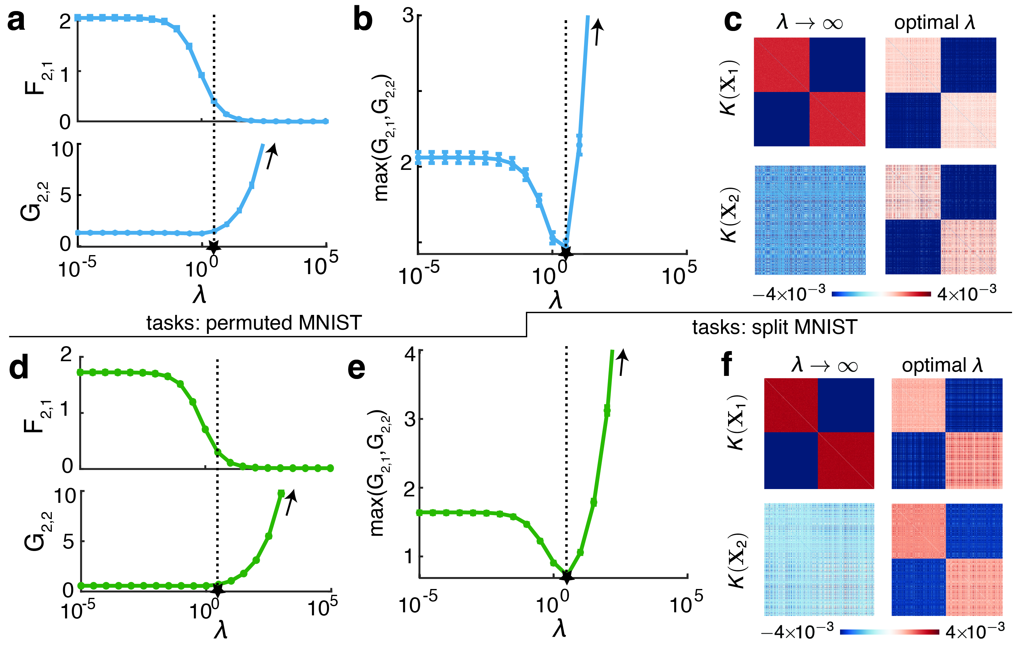
Figure 8: Optimal $\lambda$ Balances Memorization and New Learning.
a Forgetting of task 1 ($F_{2,1}$) monotonically decreases with the regularization strength ($\lambda$) while the generalization error on task 2 ($G_{2,2}$) monotonically increases. Generalization error on the first task ($G_{2,1}$) behaves similarly as $F_{2,1}$ and is not shown. The two tasks considered here are sufficiently dissimilar (permuted MNIST with 100% permutation) that they are in the overfitting regime and $G_{2,2}$ diverges at large $\lambda$.
b Maximum of the generalization error on task 1 and task 2 (max($G_{2,1}$,$G_{2,2}$)) as a function of the regularization strength $\lambda$. There exists an intermediate optimal $\lambda$ which minimizes $\max(G_{2,1},G_{2,2})$ by keeping both of them relatively small, indicated by the star. See Supplementary Note 9 for how the error can be further approximately mapped to classification accuracy.
c The learning-induced component of the similarity matrix of representations on task 1 and task 2 training data ($\bm{X}_{1}$ and $\bm{X}_{2}$), after learning the two tasks, denoted $K({\bf X}_{1})$ (top row) and $K({\bf X}_{2})$ (bottom row) respectively (Supplementary Note 2.6). At $\lambda\rightarrow\infty$, only $K(\bm{X}_{1})$ but not $K(\bm{X}_{2})$ exhibits a task-relevant block structure. This indicates that the network fails to learn good representations for task 2, and over-memorizes task 1. In contrast, at the optimal $\lambda$ (corresponding to the star in panel b), both $K(\bm{X}_{1})$ and $K(\bm{X}_{2})$ show a block structure aligned with their corresponding tasks, exhibiting a shared representation beneficial for both tasks.
d-f Same as a-c, but for split MNIST with 100% split.
In a, b, d, e, error bars are across 10 different random samples of training data. $\alpha=3$ in both examples, which is below the corresponding $\alpha_{c}$ for these sequences.

The analysis so far has shown that, when tasks are sufficiently dissimilar, $\lambda\rightarrow\infty$ can cause the network to memorize perfectly (zero $F_{2,1}$) at the expense of catastrophic anterograde interference (diverging $G_{2,2}$). We next characterized the tradeoff for such tasks between improving $G_{2,2}$ and maintaining low $F_{2,1}$ by lowering $\lambda$. As expected, as $\lambda$ lowers, the network forgets the first task more (higher $F_{2,1}$, Fig. 8a, d), resulting weaker interference of the second task (lower $G_{2,2}$, Fig. 8a, d). To evaluate the performance on both tasks and quantify the tradeoff, we also computed the test loss on task 1 after learning task 2, given by $G_{2,1}=\left\langle\mathcal{L}\left(f_{2}^{1},D_{1}^{test}\right)\right\rangle$, and studied $\max(G_{2,1},G_{2,2})$ as a function of $\lambda$ (Fig. 8b, e). We found that there exists a finite optimal $\lambda$ that minimizes $\max(G_{2,1},G_{2,2})$ by keeping both $G_{2,1}$ and $G_{2,2}$ reasonably low. Further analysis showed that empirically the optimal $\lambda$ is approximately conserved at around $O(1)$ across different task relations and load $\alpha$ (Supplementary Note 6.2).

We next sought to understand how the representations of task 1 and task 2 inputs after learning both depend on $\lambda$ by studying the representation similarity matrix after learning both tasks. Specifically, we analyzed the learned component in the similarity matrix on the training data $\bm{X}_{1}$ and $\bm{X}_{2}$ (Supplementary Note 2.6), denoted by $K(\bm{X}_{1})\in\mathbb{R}^{P\times P}$ and $K(\bm{X}_{2})\in\mathbb{R}^{P\times P}$ respectively. Prior work has indicated that, for binary classification tasks that we considered, a $2\times 2$ block structure in the similarity matrix suggests that the representations are clustered according to the task labels, and is associated with good generalization performance [41, 42, 43, 44]. Indeed, we found that at large $\lambda$, the similarity matrix has such structure for $\bm{X}_{1}$ but not $\bm{X}_{2}$ (Fig. 8c, f), explaining our previous finding that in the overfitting regime the network fails to generalize on task 2. However, when using the optimal $\lambda$ that minimizes $\max\left(G_{2,1},G_{2,2}\right)$, representations of inputs from both tasks have such block structure, consistent with the finding that both $G_{2,1}$ and $G_{2,2}$ are reasonable (Supplementary Note 6.3), highlighting the importance of representation learning on the generalization capabilities in CL.

5 Discussion

Forgetting and Task Relations

We systematically investigated how task relations influence catastrophic forgetting in $L_{2}$-regularized CL in wide DNNs in single-head and multi-head scenarios, studying both short-term forgetting (sequential learning of two tasks) and long-term forgetting (a long sequence of tasks). In contrast to prior work, which mostly treated “task similarity” as a single variable [2, 18, 45, 16, 22, 21] (but see [20, 13]), our analysis emphasizes the importance of distinguishing input and rule similarity, respectively measured by $\gamma_{input}$ and $\gamma_{rule}$. For single-head CL, they have contrasting effects on forgetting: higher input similarity increases short-term forgetting and speeds up long-term forgetting, whereas higher rule similarity reduces short-term forgetting and lowers the maximum of long-term forgetting. The relationship between the severity of forgetting and either type of similarity is monotonic, consistent with a previous toy-model analysis [13]. For multi-head CL, their effects depend on the load $\alpha$. For $\alpha<1$, task relations have no effect on forgetting as it vanishes at $\lambda\rightarrow\infty$. However, for $\alpha>1$ there exists a $\gamma_{input}-\gamma_{rule}-\alpha$ phase diagram (Fig. 7). For a fixed load ($\alpha$), when both $\gamma_{input}$ and $\gamma_{rule}$ are sufficiently high, CL is in the generalization regime where forgetting is non-zero but moderate. When either drops below some critical load ($\alpha_{c}$), CL abruptly enters the overfitting regime where forgetting is zero but generalization on the new task fails despite reaching zero training error, a surprising phenomenon we termed “catastrophic anterograde interference”. For tasks in this regime, fine-tuning $\lambda$ of the learner can reach a reasonable compromise and allow the network to perform both tasks (Fig. 8).

Architecture

Our analysis suggests that task relations are modulated by the architecture of the learner. Increasing depth effectively mitigates single-head forgetting for long task sequences (reflected in increased forgetting time constant $\tau_{F}$, Fig. 4) by reducing the overlap between task subspaces, as measured by $\gamma_{input}$. In addition, increasing the width ($N$), which we studied for multi-head CL, can also mitigate forgetting. As $N$ increases for a fixed dataset size ($P$), $\alpha$ decreases below $\alpha_{c}$. As a result, CL transitions from the generalization regime, where forgetting is finite, to the overfitting regime, where it is zero. Although the specific value of $\alpha_{c}$ depends on task relations, our theory indicates that the transition to zero forgetting is a general phenomenon. Widening the network further eventually causes $\alpha$ to drop below 1 where network features are fixed and forgetting is zero for any tasks. The observed beneficial effects of depth and width on mitigating forgetting are consistent with empirical reports of less forgetting in larger networks [46].

Anterograde Effects

In addition to forgetting (retrograde interference), we investigated anterograde aspects of CL by studying how learning one task affects the generalization performance on a subsequently learned one. Results from both single-head (Fig. 5) and multi-head (Figs. 6-8) CL indicate that anterograde interference can be severe and worsens as the tasks become less similar. For multi-head CL, this is highlighted by the catastrophic anterograde interference for dissimilar tasks. This suggests a parameter regime at $\alpha>1$ where, counter-intuitively, single-head CL performs better than multi-head (Supplementary Fig. 10). It would be interesting to verify this in a future theory of single-head CL with finite $\alpha$. The existence of diverging test loss for $\alpha>1$ suggests that increasing the width of the network (reducing $\alpha$ to a value below $1$) will have a very beneficial effect on sequential learning. While anterograde interference appears prevalent and severe in our analysis, this is partially due to the specific settings we focused on. Assuming the second task to have substantially fewer training examples than the first or a compositional structure between tasks [47] could lead to stronger transfer effects. In addition, making transitions between dissimilar tasks “smoother” by inserting intermediate datasets can mitigate anterograde interference (Supplementary Note 8).

Implications for CL in the Brain

Recent neuroscience experiments indicate that neural representations of a learned task can “drift” after learning has concluded [48, 12], raising the question of how the brain maintains stable task performance despite such drifts [49]. While a multitude of mechanisms likely underlie this phenomenon, subsequent learning of other tasks by the same neural circuits likely contributes [12]. As shown by our analysis, this can indeed occur during multi-head CL at $\alpha>1$, where representations of task 1 inputs are altered by learning the second task. Our analysis hints at how the brain may deal with this issue. Task 1 performance can be unperturbed as long as representational changes occur only in the null space of its readout, consistent with the notion that the brain orthogonalizes representations for different tasks to reduce interference [50, 51, 12]. The overfitting regime demonstrates that such orthogonality can occur without storing task 1 inputs and explicitly confining new learning in their null space, as long as the penalty on weight perturbations is sufficiently strong. To avoid the failure to generalize on task 2 in this regime, the brain may weaken the penalty, where representational changes are still mostly orthogonal to the task 1 readout but sufficient for good generalization of task 2. These results suggest the possibility of enforcing near-orthogonality between task subspaces by having a regularization-like mechanism (e.g., synaptic stabilization [11, 10]) alone with appropriately tuned penalty strength.

Our results also highlight how architectural elements of the brain can confer CL benefits. Sensory expansion, a motif often seen in sensory cortices, projects a low-dimensional input signal into a much higher-dimensional code within a large population of neurons [52]. From the perspective of multi-head CL, this may effectively increase the NN width and reduce forgetting, as discussed above. Additionally, our finding that increasing depth can mitigate forgetting may indicate an advantage of having a deep, multi-stage sensory processing system. This suggestion predicts that representations of different tasks are less similar in later stages of sensory processing [53, 54]. To assess such similarity in high-dimensional neural codes without resorting to nonlinear dimensionality-reduction techniques (e.g., [51]), it may be promising to adapt our OPs to experimental data.

Finally, it would be interesting to test whether the same connections between task relations and severity of forgetting hold in the brain. For instance, animals can be sequentially trained on a series of two-alternative forced choice tasks. In each task, the animal would need to distinguish two classes of simple stimuli with a few attributes (e.g., red striped squares vs. blue dotted triangles). Different tasks would contain different randomly generated dichotomies to ensure $\gamma_{rule}\approx 0$. Assuming animals are using a single-head-like shared behavioral readout for these tasks [55] and a regularization-like mechanism for CL, our results predict forgetting to be faster if stimuli from different tasks are made more similar (higher $\gamma_{input}$).

Extensions and Limitations

The presented theory can be extended in several important directions. First, our Gibbs formulation assumes a uniform perturbation penalty across all weights, while popular regularization-based CL methods typically use some metric to evaluate the importance of each individual weight for past performance and apply a stronger penalty to more important ones [6, 28]. Our theory may be extended to the case with weight-specific penalties and elaborate how different importance metrics affect CL outcomes. Second, there are important aspects of task relations not captured by the two specific OPs we studied. For example, our CL OPs are symmetric with respect to task ordering, preventing them from capturing how different orderings of the same set of tasks elicit different CL performance. While we have neglected ordering effects here because they are often small in common task sequences [56, 16], they may be captured by modifications of OP definitions or the addition of an “asymmetric OP” in specific setups where the ordering becomes significant (Supplementary Note 3). Finally, while we have focused on leveraging task-identity information during CL using the multi-head scheme, such information can also improve single-head CL. This may be done by appending a task-identity embedding vector to relevant inputs [57] or gate individual neurons in a task-dependent manner [58, 59, 60]. Extending our theory to analyze how these mechanisms affect the OPs and CL performance is a promising future research direction.

6 Methods

Network Architecture

All networks we studied have a fully-connected feedforward body. $\bm{x}^{l=0,...,L}$ denote the vector of activation in the $l$-th hidden layer in response to input $\bm{x}$ ($\bm{x}^{0}\equiv\bm{x}$), given by

$$x_{i}^{l+1}\left(\bm{x}\right)=\phi\left(\frac{1}{\sqrt{\text{dim}\left(\bm{x}^{l}\right)}}\sum_{j}W_{ij}^{l}x_{j}^{l}\left(\bm{x}\right)\right),$$ (8)

where $\text{dim}\left(\bm{x}^{0}\right)=N_{0}$ and $\dim\left(\bm{x}^{1,...,L}\right)=N$. The representation of an input $\bm{x}$ denotes the last-layer activation, $\Phi\left(\mathcal{W},\bm{x}\right)\equiv\bm{x}^{L}\left(\bm{x}\right)$. $\phi:\mathbb{R}\rightarrow\mathbb{R}$ is the single-neuron activation function, taken to be ReLU ($\phi(x)=\max\left\{0,x\right\}$).

Summary of Theoretical Results

This section summarizes the main theoretical results. We first introduce several important “generalized kernel functions” that play a key role in the theory, and will appear in the expressions for the network-output statistics that determine the network performance. We then introduce the expressions for the statistics of the network’s input-output mapping in the case of single-head and multi-head CL, respectively. For single-head CL, we present the expression for the average input-output mappings of the network, denoted as $\langle f_{t}\rangle$ at $t=1,\cdots,T$ for arbitrary $T$. For multi-head CL, we present both the mean and variance of the network input-output mappings, respectively denoted as $\langle f_{t}^{\tau}\rangle$ and $\langle\delta^{2}f_{t}^{\tau}\rangle$ ($t=1,\cdots,T;\tau=1,\cdots,t$), for $L=1$ and $T=2$. Further expositions of the theory can be found in Supplementary Note 1 (single-head) and Supplementary Note 2 (multi-head).

Generalized Kernel Functions

Our theoretical results show that the statistics of the network’s input-output mappings depend on the input data through several generalized kernel functions, similar in spirit to the Neural Tangent Kernel (NTK) and Neural Network Gaussian Process (NNGP) theories of learning [19, 61]. However, there are two crucial differences between the generalized kernel functions in our theory and the kernels in NTK/NNGP theories. First, our kernel functions are “generalized” in that they are generally asymmetric with respect to the inputs and thus are not proper kernels [62]. Second, our kernel functions are time-dependent, as opposed to the stationary NTK/NNGP kernels in classic results. For brevity, we simply refer to the generalized kernel functions as kernels or kernel functions hereafter.

The kernel functions are defined as the inner products between random features averaged over correlated Gaussian weights. The statistics of the Gaussian weights are given by the prior contribution in Eq. 3, specifically

$$P(\mathcal{W})\propto\exp\left(-\frac{1}{2}\beta^{-1}\sigma^{-2}\sum_{t=1}^{T}\left\|\mathcal{W}_{t}\right\|^{2}+\frac{1}{2}\beta^{-1}\sum_{t=2}^{T}\lambda\left\|\mathcal{W}_{t}-\mathcal{W}_{t-1}\right\|^{2}\right)$$ (9)

Kernel functions for arbitrary $\lambda$:

The important kernel functions are given by

$$K_{t,t^{\prime}}^{L,1}(\bm{x},\bm{x}^{\prime})\equiv\frac{1}{N}\langle\Phi(\mathcal{W}_{t},\bm{x})\cdot\Phi(\mathcal{W}_{t^{\prime}},\bm{x}^{\prime})\rangle_{\mathcal{W}}$$ (10)

$$K_{t,t^{\prime}}^{L,0}(\bm{x},\bm{x}^{\prime})\equiv\frac{1}{N}\langle\langle\Phi(\mathcal{W}_{t},\bm{x})\rangle_{t,t^{\prime}}\cdot\langle\Phi(\mathcal{W}_{t^{\prime}},\bm{x}^{\prime})\rangle_{t^{\prime},t^{\prime}}\rangle_{\mathcal{W}}$$ (11)

where $\langle\cdot\rangle_{\mathcal{W}}$ denotes the average over the full prior distribution Eq. 9, and $\langle\cdot\rangle_{t,t^{\prime}}$ denotes the partial average over the conditional distribution $P(\mathcal{W}_{t,}\mathcal{W}_{t-1},\cdots,\mathcal{W}_{t^{\prime}}|\mathcal{W}_{t^{\prime}-1})$. Furthermore, we introduce

$$\tilde{K}_{t,t^{\prime}}^{L}(\bm{x},\bm{x}^{\prime})\equiv m_{t,t^{\prime}}^{1}K_{t,t^{\prime}}^{L,1}(\bm{x},\bm{x}^{\prime})-m_{t,t^{\prime}}^{0}K_{t,t^{\prime}}^{L,0}(\bm{x},\bm{x}^{\prime})$$ (12)

For $t\geq t^{\prime}\geq 2$, $m_{t,t^{\prime}}^{1}=\frac{\sigma^{2}}{1+\tilde{\lambda}}(\tilde{\lambda}^{t-t^{\prime}}+\tilde{\lambda}^{t+t^{\prime}-1})$, and $m_{\tau,\tau^{\prime}}^{0}=\frac{\sigma^{2}}{1+\tilde{\lambda}}(\tilde{\lambda}^{t-t^{\prime}+2}+\tilde{\lambda}^{t+t^{\prime}-1})$, where $\tilde{\lambda}\equiv\lambda(\lambda+\sigma^{-2})^{-1}$. Otherwise, $m_{t,1}^{1}=\sigma^{2}\tilde{\lambda}^{t-1}$ and $m_{t,1}^{0}=0$. Finally, we introduce the difference kernel

$$\Delta K_{t,t^{\prime}}^{L}(\bm{x},\bm{x}^{\prime})\equiv K_{t,t^{\prime}}^{1}(\bm{x},\bm{x}^{\prime})-K_{t,t^{\prime}}^{0}(\bm{x},\bm{x}^{\prime}).$$ (13)

Kernel functions in the $\lambda\rightarrow\infty$ limit:

In the limit $\lambda\rightarrow\infty$, these kernel functions become stationary in time and can be simplified. In particular, $K_{t,t^{\prime}}^{L,1}(\bm{x},\bm{x}^{\prime})$ becomes the NNGP kernel, given by

$$K_{t,t^{\prime}}^{L,1}(\bm{x},\bm{x}^{\prime})\overset{\lambda\rightarrow\infty}{\longrightarrow}K_{GP}^{L}(\bm{x},\bm{x}^{\prime})\equiv\Phi(\mathcal{W}_{0},\bm{x})\cdot\Phi(\mathcal{W}_{0},\bm{x}^{\prime}),$$ (14)

where $\Phi(\mathcal{W}_{0},\bm{x})\in\mathbb{R}^{N}$, and $\mathcal{W}_{0}\sim\mathcal{N}(0,\sigma^{2}\mathbb{I})$, as introduced in the main text when we introduced the OPs. $\tilde{K}_{t,t^{\prime}}^{L}$ ($t,t^{\prime}\geq 2$) becomes the NTK, given by

$$\tilde{K}_{t,t^{\prime}}^{L}(\bm{x},\bm{x}^{\prime})\overset{\lambda\rightarrow\infty}{\longrightarrow}\lambda^{-1}K_{NTK}^{L}(\bm{x},\bm{x}^{\prime})\equiv\lambda^{-1}\partial_{\Theta_{random}}f(\Theta_{0},\bm{x})\cdot\partial_{\Theta_{random}}f(\Theta_{0},\bm{x}^{\prime})$$ (15)

where $\partial_{\Theta_{0}}f(\Theta_{0},\bm{x})\in\mathbb{R}^{N^{2}(L-1)+NN_{0}+N}$ is of the dimension of the total number of parameters in the network, and $\Theta_{0}\sim\mathcal{N}(0,\sigma^{2}\mathbb{I}).$ $\Delta K_{t,t^{\prime}}^{L}(\bm{x},\bm{x}^{\prime})$ is given by

$$\Delta K_{t,t^{\prime}}^{L}(\bm{x},\bm{x}^{\prime})\overset{\lambda\rightarrow\infty}{\longrightarrow}\lambda^{-1}K_{NTK}^{L}(\bm{x},\bm{x}^{\prime})\dot{K}^{L}(\bm{x},\bm{x}^{\prime})$$ (16)

where

$$\dot{K}^{L}(\bm{x},\bm{x}^{\prime})\equiv\phi^{\prime}(h_{0}^{L}(\bm{x}))\cdot\phi^{\prime}(h_{0}^{L}(\bm{x}^{\prime}))$$ (17)

is the derivative kernel. $\left\{h_{0}^{l}(\bm{x})\right\}_{l=1,\cdots,L}$ denote the pre-activation of each layer with random weights $\mathcal{W}_{0}=\left\{W_{0}^{l}\right\}_{l=1,\cdots,L}$, i.e.,

$$h_{0}^{l}(\bm{x})\equiv\frac{1}{\sqrt{\text{dim}\left(\bm{x}^{l-1}\right)}}\sum_{j}W_{0,ij}^{l-1}x_{0,j}^{l-1}\left(\bm{x}\right)$$ (18)

$$x_{0}^{l}(\bm{x})=\phi(h_{0}^{l}(\bm{x}))$$ (19)

In the infinite-width limit $N\rightarrow\infty$, Eqs. 14-17 are all self-averaging, namely, they do not depend on the specific realization of $\mathcal{W}_{0}$ or $\Theta_{0}$, and is equivalent to their averages across Gaussian $\mathcal{W}_{0}$ or $\Theta_{0}$. See Supplementary Note 1.2 for detailed derivations of the kernel functions and Supplementary Note 1.4 for their analytical expressions in ReLU networks.

Furthermore, to simplify the expression of the statistics of the network’s input-output mappings, for each kernel function, we introduce corresponding notations for applying them to the training and testing data, respectively. Specifically, for a kernel function $K_{t,t^{\prime}}^{L}(\bm{x},\bm{x}^{\prime})$, we introduce

$$\bm{k}_{t,t^{\prime}}^{L}(\bm{x})\equiv K_{t,t^{\prime}}^{L}(\bm{x},\bm{X}_{t^{\prime}})\in\mathbb{R}^{P}$$ (20)

$$\bm{K}_{t,t^{\prime}}^{L}\equiv K_{t,t^{\prime}}^{L}(\bm{X}_{t},\bm{X}_{t^{\prime}})\in\mathbb{R}^{P\times P}$$ (21)

$$k_{t,t^{\prime}}^{L}\equiv K_{t,t^{\prime}}^{L}(\bm{x},\bm{x})\in\mathbb{R}$$ (22)

where $\bm{X}_{t}$ denotes the training data matrix of task $t$, and $\bm{x}$ denotes an arbitrary test point. $K^{L}$ represents the different kernel functions above, including $K^{L,1},K^{L,0},\tilde{K}^{L}$ and $\Delta K^{L}$.

Single-Head Theory

In single-head CL, the mean input-output mapping after learning $T$ tasks in a network with $L$ hidden layers in the infinite-width limit ($N\rightarrow\infty$, $\alpha=P/N\rightarrow 0$) is given by

$$\langle f_{T}(\bm{x})\rangle=\sum_{t=1}^{T}\tilde{\bm{k}}_{T,t}^{L}(\bm{x})^{\top}\langle-i\bm{v}_{t}\rangle$$ (23)

$$\langle-i\bm{v}_{t}\rangle=\left(\tilde{\bm{K}}_{t,t}^{L}\right)^{-1}(\bm{Y}_{t}-\sum_{t^{\prime}=1}^{t-1}\tilde{\bm{K}}_{t,t^{\prime}}^{L}\langle-i\bm{v}_{\tau^{\prime}}\rangle)$$ (24)

The equation is applied to evaluate $F_{t,1}\approx\mathcal{L}(\langle f_{T}\rangle,D_{1})$ (relevant results shown in Figs. 2-4) and $G_{2,2}\approx\mathcal{L}(\langle f_{2}\rangle,D_{2}^{test})$ (relevant results shown in Fig. 5). These results hold for general $\lambda$, in the $\lambda\rightarrow\infty$ limit, the kernels $\tilde{K}_{t,t^{\prime}}^{L}(t,t^{\prime}\geq 2)$ are replaced with $\lambda^{-1}K_{NTK}^{L}$ (Eq. 15) and the kernels $\tilde{K}_{t,1}^{L}$ are replaced with $K_{GP}^{L}$ (Eq. 14). All results shown use $\sigma^{2}=0.04$ such that the variance of the mapping (expression derived in Supplementary Note 1.3) becomes negligible.

Multi-Head Theory

In multi-head CL, we consider both the mean and variance of the network’s input-output mappings, for $T=2$ and $L=1$. The variance is not negligible as in single-head CL, as it causes the divergent $G_{2,2}$ in the overfitting regime. We thus neglect the $L$ superscript of the kernels in this section. Analogous to the kernel $\tilde{K}_{t,t^{\prime}}^{L}(\bm{x},\bm{x}^{\prime})$ defined in Eq. 12, we introduce a new “renormalized” kernel for multi-head CL, using the same notation

$$\tilde{K}_{2,2}(\bm{x},\bm{x}^{\prime})\equiv u_{2,2}^{1}K_{2,2}^{1}(\bm{x},\bm{x}^{\prime})-u_{2,2}^{0}K_{2,2}^{0}(\bm{x},\bm{x}^{\prime})$$ (25)

where the “renormalization factors” $u_{2,2}^{1}$ and $u_{2,2}^{0}$ can be solved self-consistently as detailed in Supplementary Note 2.3. Similarly as in the earlier section where we introduced the single-head theory, we introduce $\tilde{\bm{k}}_{2,2}(\bm{x})\in\mathbb{R}^{P},\tilde{\bm{K}}_{2,2}\in\mathbb{R}^{P\times P}$ and $\tilde{k}_{2,2}\in\mathbb{R}$ for this kernel function applied on the training and testing data. The expressions for the statistics of the network’s input-output mappings are given as follows.

Mean of $f$:

The mean input-output mappings are given by

$$\langle f_{2}^{1}(\bm{x})\rangle =u_{1,2}^{1}\Delta\bm{k}_{2,2}(\bm{x})^{\top}\tilde{\bm{K}}_{2,2}^{-1}\left(\bm{Y}_{2}-u_{1,2}^{1}\left(u_{1,1}^{1}\right)^{-1}\bm{K}_{2,1}^{1}\left(\bm{K}_{1,1}^{1}\right)^{-1}\bm{Y}_{1}\right)+\bm{k}_{2,1}^{1}(\bm{x})^{\top}\left(\bm{K}_{1,1}^{1}\right)^{-1}\bm{Y}_{1}$$ (26)

$$\langle f_{2}^{2}(\bm{x})\rangle =\tilde{\bm{k}}_{2,2}(\bm{x})^{\top}\tilde{\bm{K}}_{2,2}^{-1}\left(\bm{Y}_{2}-u_{1,2}^{1}\left(u_{1,1}^{1}\right)^{-1}\bm{K}_{2,1}^{1}\left(\bm{K}_{1,1}^{1}\right)^{-1}\bm{Y}_{1}\right)+u_{2,1}^{1}\left(u_{1,1}^{1}\right)^{-1}\bm{k}_{2,1}^{1}(\bm{x})^{\top}\left(\bm{K}_{1,1}^{1}\right)^{-1}\bm{Y}_{1}$$ (27)

Variance of $f$:

The variance of the input-output mappings are

$$\langle\delta f_{2}^{1}(\bm{x})^{2}\rangle =u_{1,1}^{1}k_{2,2}^{1}(\bm{x},\bm{x})-\left(u_{1,2}^{1}\right)^{2}\Delta\bm{k}_{2,2}(\bm{x})^{\top}\tilde{\bm{K}}_{2,2}^{-1}\Delta\bm{k}_{2,2}(\bm{x})-\left(u_{1,1}^{1}\bm{k}_{2,1}^{1}(\bm{x})-u_{1,2}^{1}\Delta\bm{k}_{2,2}(\bm{x})\tilde{\bm{K}}_{2,2}^{-1}\tilde{\bm{K}}_{2,1}\right)\tilde{\bm{K}}_{1,1}^{-1}$$

$$\left(u_{1,1}^{1}\bm{k}_{2,1}^{1}(\bm{x})-u_{1,2}^{1}\Delta\bm{k}_{2,2}(\bm{x})\tilde{\bm{K}}_{2,2}^{-1}\tilde{\bm{K}}_{2,1}\right)^{\top}-2\left(u_{1,2}\right)^{2}\Delta\bm{k}_{2,2}(\bm{x})\tilde{\bm{K}}_{2,2}^{-1}\bm{k}_{2,2}^{0}(\bm{x})^{\top}$$

$$+\left(u_{1,2}^{1}\right)^{2}u_{2,2}^{0}\Delta\bm{k}_{2,2}(\bm{x})^{\top}\tilde{\bm{K}}_{2,2}^{-1}\bm{K}_{2,2}^{0}\tilde{\bm{K}}_{2,2}^{-1}\Delta\bm{k}_{2,2}(\bm{x})$$ (28)

$$\langle\delta f_{2}^{2}(\bm{x})^{2}\rangle =u_{2,2}^{1}k_{2,2}^{1}(\bm{x},\bm{x})-\left(u_{2,2}^{1}\right)^{2}\Delta\bm{k}_{2,2}(\bm{x})^{\top}\tilde{\bm{K}}_{2,2}^{-1}\Delta\bm{k}_{2,2}(\bm{x})-\left(\tilde{\bm{k}}_{2,1}(\bm{x})-\tilde{\bm{k}}_{2,2}(\bm{x})\tilde{\bm{K}}_{2,2}^{-1}\tilde{\bm{K}}_{2,1}\right)\tilde{\bm{K}}_{1,1}^{-1}$$

$$\left(\tilde{\bm{k}}_{2,1}(\bm{x})-\tilde{\bm{k}}_{2,2}(\bm{x})\tilde{\bm{K}}_{2,2}^{-1}\tilde{\bm{K}}_{2,1}\right)^{\top}-2u_{2,2}^{0}\tilde{\bm{k}}_{2,2}(\bm{x})\tilde{\bm{K}}_{2,2}^{-1}\bm{k}_{2,2}^{0}(\bm{x})^{\top}$$

$$+u_{2,2}^{0}\tilde{\bm{k}}_{2,2}(\bm{x})\tilde{\bm{K}}_{2,2}^{-1}\bm{K}_{2,2}^{0}\tilde{\bm{K}}_{2,2}^{-1}\tilde{\bm{k}}_{2,2}(\bm{x})^{\top}.$$ (29)

These results hold for arbitrary $\lambda$. The “renormalization factors” $\left\{u_{1,1}^{1},u_{1,2}^{1},u_{2,2}^{1},u_{2,2}^{0}\right\}$ are solved with Supplementary Eqs. 119, 122 in Supplementary Note 2.3. We can then plug them back into Eqs. 26, 29, and use them to evaluate $F_{2,1}=\left\langle\mathcal{L}(f_{2}^{1},D_{1})\right\rangle$, $G_{2,2}=\left\langle\mathcal{L}(f_{2}^{2},D_{2}^{test})\right\rangle$ and $G_{2,1}=\left\langle\mathcal{L}(f_{2}^{1},D_{1}^{test})\right\rangle$, which we show in our multi-head results.
Furthermore, in the $\lambda\rightarrow\infty$ limit, the phase-transition boundary between the overfitting regime and the generalization regime and the corresponding $\alpha_{c}$ (shown in Figs. 6, 7) is calculated by solving

$$\gamma_{asymm}\gamma_{1}\gamma_{input}-\gamma_{rule}^{2}\gamma_{1}>u_{1,1}^{1}\left(\gamma_{input}-\alpha^{-1/2}\right)$$ (30)

$$\sigma^{-2}\left(u_{1,1}^{1}\right)^{2}-(1-\alpha)u_{1,1}^{1}-\alpha\gamma_{1}=0$$ (31)

where we have defined $\gamma_{1}\equiv\lVert\bm{V}_{1}\rVert^{2}$, along with several important order parameters. $\gamma_{input}$ and $\gamma_{rule}$ are defined in Eqs. 6, 5, and an additional OP $\gamma_{asymm}$ is given by

$$\gamma_{asymm}\equiv\gamma_{1}^{-1}\gamma_{input}^{-1}\bm{V}_{1}^{\top}\bm{P}_{2}\bm{V}_{1}$$ (32)

For details of different solutions of the renormalization factors in the three phases, and the derivations of the phase-transition boundary see Supplementary Note 2.5, for further discussion about $\gamma_{asymm}$ see Supplementary Note 3. Theoretical results regarding the hidden representations (Fig. 8c, f) are shown in Supplementary Note 2.6. All multi-head CL results shown are evaluated with $\sigma^{2}=1$, results for the $\lambda\rightarrow\infty$ limit are evaluated at $\lambda=10^{6}$.

Student-Teacher Setting with Parametric Task Relations

The student-teacher setting is based on the template model [52], where the training inputs of each task consists of $P$ templates and the test inputs are sampled near these templates with Gaussian noise of variance $\sigma_{x}^{2}$. To generate $T$ sets of training inputs with the desired cross-task correlation controlled by $\rho_{input}$, we first sample $\left\{\bm{g}_{t}^{\mu}\right\}_{t=0,...,T;\mu=1,...P}$ i.i.d. from $\mathcal{N}\left(0,\left(1-\sigma_{x}^{2}\right)\mathbb{I}_{N_{0}}\right)$. Training examples for the $t$-th task are then given by $\bm{x}_{t}^{\mu}=\sqrt{\rho_{input}}\bm{g}_{0}^{\mu}+\sqrt{1-\rho_{input}}\bm{g}_{t}^{\mu}.$

Labels for training and test inputs for task $t$ are generated with $y_{t}^{\mu}=f_{t}^{teacher}\left(\bm{x}_{t}^{\mu}\right)$, where each of $\left\{f_{t}^{teacher}\right\}_{t=1,...,T}$ is the input-output mapping of a two-layer ReLU network with random weights and $N_{teacher}$ neurons in the hidden layer. All teacher networks share the same random hidden-layer weights, which are sampled i.i.d. from $\mathcal{N}\left(0,1\right)$. Readout weights from different teachers have pairwise correlation controlled by the teacher similarity parameter $\rho_{teacher}$. Readout weights are generated in a way analogous to how $\left\{\bm{x}_{t}^{\mu}\right\}_{t=1,\cdots T;\mu=1,\cdots,P}$ are generated above. Finally, we add a fixed scalar bias to the output of each network such that $\left\langle f_{t}^{teacher}\left(\bm{x}\right)\right\rangle_{\bm{x}\sim\mathcal{N}\left(0,\mathbb{I}\right)}=0$.

Figs. 2, 3 were produced with $L=1,P=100,N_{0}=100,N_{teacher}=100,\sigma_{x}^{2}=0$. We used $\sigma_{x}^{2}=0$ because these analyses do not concern the test sets. Figs. 6 and 7a were produced with $L=1,P=600,N_{0}=300,N_{teacher}=300,\sigma_{x}^{2}=0.5$.

Computing Order Parameters

We here discuss how the OPs are computed for ReLU architectures of a given depth. We assume $\mathcal{W}_{0}$ to be drawn i.i.d. from a Gaussian distribution, $\mathcal{N}\left(0,\sigma^{2}\mathbb{I}\right)$. For the NNs we studied, which have ReLU nonlinearity and no bias terms, the OPs do not depend on the variance of $\mathcal{W}_{0}$ (explained below). In the large $N$ limit, the OPs are deterministic functions of the datasets $\left\{\left(\bm{X}_{i},\bm{Y}_{i}\right)\right\}_{i\in\{A,B\}}$ and the depth of the NN. In other words, they do not fluctuate with different samples of $\mathcal{W}_{0}$ In addition, they can be computed without handling vectors and matrices of $N$ dimensions, which is not feasible under the $N\rightarrow\infty$ assumption.

Input Similarity $\gamma_{input}$ (Eq. 5):

By invariance of the trace operator to circular shifts,

$$\gamma_{input} =\frac{\text{Tr}\left(\left[\bm{X}_{A}^{L}\left(\bm{X}_{A}^{L}\right)^{T}\right]^{-1}\bm{X}_{A}^{L}\left(\bm{X}_{B}^{L}\right)^{T}\left[\bm{X}_{B}^{L}\left(\bm{X}_{B}^{L}\right)^{T}\right]^{-1}\bm{X}_{B}^{L}\left(\bm{X}_{A}^{L}\right)^{T}\right)}{\sqrt{\prod_{i=A,B}\text{Tr}\left(\left[\bm{X}_{i}^{L}\left(\bm{X}_{i}^{L}\right)^{T}\right]^{-1}\bm{X}_{i}^{L}\left(\bm{X}_{i}^{L}\right)^{T}\right)}}.$$

The NNGP kernel can be written as $K_{GP}^{L}\left(\bm{X}_{i},\bm{X}_{j}\right)=N^{-1}\bm{X}_{i}^{L}\left(\bm{X}_{j}^{L}\right)^{T}\in\mathbb{R}^{P\times P}$ , equivalent to Eq. 14, we can write

$$\gamma_{input}=\frac{\text{Tr}\left(K_{GP}^{L}\left(\bm{X}_{A},\bm{X}_{A}\right)^{-1}K_{GP}^{L}\left(\bm{X}_{A},\bm{X}_{B}\right)K_{GP}^{L}\left(\bm{X}_{B},\bm{X}_{B}\right)^{-1}K_{GP}^{L}\left(\bm{X}_{B},\bm{X}_{A}\right)\right)}{P}.$$ (33)

As already mentioned in Methods, at large $N$ and under our assumption of weight statistics, $K_{GP}^{L}\left(\bm{X}_{i},\bm{X}_{j}\right)$ is a deterministic function of $\bm{X}_{i},\bm{X}_{j}$. This kernel function is available with explicit iterative expressions for ReLU networks (given in [61] and Supplementary Note 1.4), allowing for $\gamma_{input}$ to be easily computed. For ReLU networks, changing the variance of $\mathcal{W}_{0}$ amounts to scaling all $K_{GP}^{L}$ by the same factor [61], which cancels out in the expressions for $\gamma_{input}$, $\gamma_{rule}$. Thus, without loss of generality, we can assume the variance $\sigma^{2}$ to be 1.

Rule Congruency $\gamma_{rule}$ (Eq. 6):

$\gamma_{rule}$ can be similarly expressed in terms of $K_{GP}^{L}$ as

$$\gamma_{rule} =\frac{\bm{Y}_{A}^{T}\left[\bm{X}_{A}^{L}\left(\bm{X}_{A}^{L}\right)^{T}\right]^{-1}\bm{X}_{A}^{L}\left(\bm{X}_{B}^{L}\right)^{T}\left[\bm{X}_{B}^{L}\left(\bm{X}_{B}^{L}\right)^{T}\right]^{-1}\bm{Y}_{B}}{\prod_{i=A,B}\sqrt{\bm{Y}_{i}^{T}\left[\bm{X}_{i}^{L}\left(\bm{X}_{i}^{L}\right)^{T}\right]^{-1}\bm{X}_{i}^{L}\left(\bm{X}_{i}^{L}\right)^{T}\left[\bm{X}_{i}^{L}\left(\bm{X}_{i}^{L}\right)^{T}\right]^{-1}\bm{Y}_{i}}}$$

$$=\frac{\bm{Y}_{A}^{T}K_{GP}^{L}\left(\bm{X}_{A},\bm{X}_{A}\right)^{-1}K_{GP}^{L}\left(\bm{X}_{A},\bm{X}_{B}\right)K_{GP}^{L}\left(\bm{X}_{B},\bm{X}_{B}\right)^{-1}\bm{Y}_{B}}{\prod_{i=A,B}\sqrt{\bm{Y}_{i}^{T}K_{GP}^{L}\left(\bm{X}_{i},\bm{X}_{i}\right)^{-1}\bm{Y}_{i}}}.$$

See Supplementary Notes 1.6 and 2.5 for how these OPs arise from our theory of single-head and multi-head CL, respectively.

Benchmark Task Sequences

All source datasets used (MNIST [33], EMNIST [34], Fashion-MNIST [35], and CIFAR-100 [36]) are image classification datasets. The images are either grayscale (MNIST, EMNIST, Fashion-MNIST) or converted to grayscale (CIFAR-100). As preprocessing, all images are centered (zero-meaned), whitened, and normalized (such that the squared norm of every image is the input dimension of each source dataset). While each source dataset contains $\mathcal{O}(10^{5})$ images in total, all of our analysis used subsets of $\mathcal{O}\left(10^{2}-10^{3}\right)$ images to save computational cost, as commonly done in theoretical studies of deep NNs (e.g., [19, 63]) – the subset of images used are redrawn for each random seed used. The specific protocols used for generating task sequences from source datasets are detailed below. In all cases we use the MNIST dataset, which consists of images of digits “0” through “9”, as an example to explain the protocols.

Permutation

Our permutation protocol largely follows standard practices in the literature [2]. Each source dataset is first turned into a binary classification dataset by randomly dividing the original image classes (e.g., “0” through “9”) into two groups. Images from one group are assigned target label $+1$ and those from the other are assigned $-1$. All training and test images corresponding to the same task undergo the same randomly generated pixel permutation, where the fraction of pixels permuted (relative to the original unpermuted images) is termed the “permutation ratio”. The permutation is independently generated for each task. Inputs in each of $D_{1},...,D_{T}$ are permuted versions of the same subset of images – this allows us to fully explore the range of input similarity, since at zero permutation $D_{1}=D_{2}=...=D_{T}$.
Note that the protocol above differs from standard practices in that we also permuted images in $D_{1}$ – this to ensure such that any pair of tasks in a long sequence (Fig. 4) have the same statistical relations. In all analysis of forgetting over permutation sequences of two tasks (Fig. 7), we followed standard practices and did not permuted $D_{1}$. $P=500$ in Fig. 4; $P=600$ in Figs. 7, 8. In the two examples of permuted MNIST in Fig. 7, images for the second task are permuted at 5% (lighter line) and 15% (darker line). In the example in Fig. 8, images for the second task are permuted 100%.

Split

Our split protocol also largely follows standard practices in the literature [2, 28]. Each task contains only images from a disjoint pair of classes (e.g., task 1 is “0” vs. “1”, task 2 is “2” vs. “3”). Thus, the maximum length of the sequence is limited by the number of classes in the source dataset – since MNIST and Fashion-MNIST each contains 10 classes, they can produce sequences with at most five tasks. On the other hand, CIFAR-100 contains 100 classes and EMNIST contains 62 classes, allowing for much longer sequences. Thus, our analysis of long-term forgetting (Fig. 4) only applies the split protocol to CIFAR-100 and EMNIST. Each random seed corresponds to a different subsample of images from each class being used, as well as a random assignment of classes into pairs.

In the special case of having only two tasks (Figs. 7, 8), we designed a “partial split” protocol to parametrically vary relations between $D_{1}$ and $D_{2}$. As an example, suppose the first pair of classes is “0” and “1”. The second pair is “2” and “3”. Under $x\%$ split, the training/test sets of task 1 would have $\left(x/2+50\right)\%$ images from the first pair and $\left(-x/2+50\right)\%$ from the second pair, whereas task 2 would have $\left(-x/2+50\right)\%$ from the first and $\left(x/2+50\right)\%$ from the second. Images in both tasks are labeled according to the rule “0”, “1” vs. “2”, “3”. Under $0\%$ split the two datasets would be identical.

In Fig. 4, we used the regular split protocol and $P=500$. In Figs. 7, 8, we used the partial-split approach to adjust the similarity for split MNIST, and fixed $P=600$ for each task. The split ratio is 25% (darker line) and 15% (lighter line) in the two examples in Fig. 7 and 0% in Fig. 8.

Label Flipping

This protocol produces two tasks. Inputs in each dataset are sampled from all original classes. Labels for images in each task are determined according to a different rule. In the case of zero flipping, both tasks use the same rule to dichotomize original classes. An example task sequence generated with partial flipping would include task 1 with “0” through “4” vs. “5” through “9” and task 2 with “0”, “1”, “2”, “3”, “5” vs. “4”, “6”, “7”, “8”, “9”.

Importantly, each of $D_{1},D_{2}$ contains an independently drawn subset of images, unlike in the permutation protocol. Therefore, $D_{1}\neq D_{2}$ even without label flipping. This is important for the analysis of anterograde effects since, if we have used the exact same images for both $D_{1},D_{2}$, there would be zero knowledge transfer even without label flipping. We used $P=500$.

Measuring Generalization

For all analysis measuring the generalization performance of an NN (Figs. 5-8), we restricted the source dataset to be either MNIST or Fashion-MNIST. This is motivated by our observation, consistent with reports from others [61, 64], that fully-connected networks in general have poor single-task generalization performance on CIFAR-100 and EMNIST. On the other hand, performance on MNIST and Fashion-MNIST is more reasonable.

Exponential Fitting of Long-Term Forgetting

Let $F_{t=1,...,T}$ be the forgetting on task 1. All exponential fitting was carried out on the forgetting averaged over data randomness, $\bar{F}_{t=1,...,T}$. In the student-teacher setting, data randomness refers to random variables such as teacher-network weights. For benchmark task sequences, it refers factors such as different subsamples of the full source dataset (see Methods). For permutation task sequences with very low permutation ratios, we sometimes observed a non-monotonic relation between $\bar{F}_{t}$ and $t$. In these cases we truncated $\bar{F}_{t=1,...,T}$ at the maximum before fitting.

7 Acknowledgements

The authors would like to thank Alexander van Meegen and Daniel D. Lee for helpful discussions. This research is supported by the Swartz Foundation, the Gatsby Charitable Foundation, the Kempner Institute for the Study of Natural and Artificial Intelligence at Harvard University, and Office of Naval Research (ONR) grant No. N0014-23-1-2051.

Supplementary Information

1 Single-Head Theory

1.1 Moment Generating Function

In this section, we present the detailed derivation for the statistics of input-output mappings in single-head CL in the infinite-width limit. We start from the MGF for multi-head CL, given by

$$\mathcal{M}(\ell_{T})\equiv\left[Z(D_{1})\prod_{t=2}^{T}Z\left(\Theta_{t-1},D_{t}\right)\right]^{-1}\exp\left(-\beta E(\Theta_{1}|D_{1})-\sum_{t=2}^{T}\beta E\left(\Theta_{t}|\Theta_{t-1},D_{t}\right)+i\sum_{t=1}^{T}\ell_{T}f_{T}({\bf x})\right)$$ (1)

where

$$E\left(\Theta_{t}|\Theta_{t-1},D_{t}\right)=\frac{1}{2}\sum_{\mu=1}^{P}\left(f_{t}\left(\bm{x}_{t}^{\mu}\right)-y_{t}^{\mu}\right)^{2}+\frac{1}{2}\beta^{-1}\sigma^{-2}\left\|\Theta_{t}\right\|^{2}+\frac{1}{2}\beta^{-1}\lambda\left\|\Theta_{t}-\Theta_{t-1}\right\|^{2}.$$ (2)

$$E(\Theta_{1},D_{1})=\frac{1}{2}\sum_{\mu=1}^{P}\left(f_{2}^{1}\left(\bm{x}_{1}^{\mu}\right)-y_{1}^{\mu}\right)^{2}+\frac{1}{2}\beta^{-1}\sigma^{-2}\left\|\Theta_{1}\right\|^{2}$$ (3)

and

$$Z\left(\Theta_{t-1},D_{t}\right)\equiv\int d\Theta_{t}\exp(-\beta E(\Theta_{t}|\Theta_{t-1},D_{t}))$$ (4)

$$Z(D_{1})\equiv\int d\Theta_{1}\exp(-\beta E(\Theta_{1},D_{1})$$ (5)

Here we introduced field $\ell_{T}$ coupled to the mapping after learning all $T$ tasks, the statistics of $f_{T}({\bf x})$ can therefore be calculated by

$$\langle f_{T}({\bf x})\rangle=-i\frac{\partial\mathcal{M}(\ell_{T})}{\partial\ell_{T}}\lvert_{\ell_{T}=0}$$ (6)

$$\langle\delta^{2}f_{T}({\bf x})\rangle=-\frac{\partial^{2}\mathcal{M}(\ell_{T})}{\partial(\ell_{T})^{2}}\lvert_{\ell_{T}=0}$$ (7)

We use the replica method for the denominator in Supplementary Eq. 1, and denote the physical copy of $\Theta_{t}$ as $\Theta_{t}^{n}$,we have

$$Z(\Theta_{t-1},D_{t})^{-1}=Z(\Theta_{t-1}^{n},D_{t})^{-1}=\lim_{n\rightarrow 0}\int\prod_{\alpha=1}^{n-1}d\Theta_{t}^{\alpha}\exp(-\beta\sum_{\alpha=1}^{n-1}E_{t}(\Theta_{t}^{\alpha}|\Theta_{t-1}^{n},D_{t})).$$ (8)

We then introduce auxiliary integration variable $\left\{\bm{v}_{t}^{\alpha}\right\}_{t=2,\cdots,T;\alpha=1,\cdots n},\bm{v}_{1}^{n}\in\mathbb{R}^{P}$ using the H-S transform, and arrive at

$$\mathcal{M}\left(\ell_{T}\right) =\lim_{n\rightarrow 0}\intop\prod_{\alpha=1}^{n}\prod_{t=2}^{T}d\bm{v}_{t}^{\alpha}\int d\bm{v}_{1}^{n}\int\prod_{\alpha=1}^{n}\prod_{t=2}^{T}d\Theta_{t}^{\alpha}\int d\Theta_{1}^{n}\exp(-i\sum_{t,\alpha}\sum_{\mu=1}^{P}v_{t}^{\alpha,\mu}\left(f_{t}\left(\Theta_{t}^{\alpha},\bm{x}_{t}^{\mu}\right)-y_{t}^{\mu}\right)$$

$$-\frac{1}{2}\sigma^{-2}\sum_{t,\alpha}\left\|\Theta_{t}^{\alpha}\right\|^{2}-\frac{1}{2}\lambda\sum_{t=2}^{T}\sum_{\alpha=1}^{n}\left\|\Theta_{t}^{\alpha}-\Theta_{t-1}^{n}\right\|^{2}-\frac{1}{2}\beta^{-1}\sum_{t,\alpha}\bm{v}_{t}^{\alpha\top}\bm{v}_{t}^{\alpha}+\sum_{t=1}^{T}\ell_{T}f_{T}(\Theta_{T}^{n},\bm{x}))$$ (9)

where we use $f_{t}\left(\Theta_{t}^{\alpha},\bm{x}_{t}^{\mu}\right)$ to denote the mapping with the replicated $\Theta_{t}^{\alpha},$$f_{t}(\Theta_{t}^{\alpha},{\bf x}_{t}^{\mu})\equiv\frac{1}{\sqrt{N}}\bm{a}_{t}^{\alpha}\Phi(\mathcal{W}_{t}^{\alpha},{\bf x}_{t}^{\mu})$; and we use $f_{T}(\Theta_{T}^{n},\bm{x})$ to denote the mapping after learning all $T$ tasks on arbitrary test input $\bm{x}$. Note that $t=1$ is different from other time indices as we do not introduce replica for $Z_{1}(D_{1})$. Therefore only $\Theta_{1}^{n}$ (and thus $\bm{v}_{1}^{n}$) appears in the MGF. For notational convenience we define $\sum_{t,\alpha}(\cdot)_{t,\alpha}\equiv(\cdot)_{1,n}+\sum_{t=2}^{T}\sum_{\alpha=1}^{n}(\cdot)_{t,\alpha}.$

We then integrate the readout weights $\left\{\bm{a}_{t}^{\alpha}\right\}_{t=1,\cdots T;\alpha=1,\cdots n}$, and obtain in the $\beta\rightarrow\infty$ limit

$$\mathcal{M}\left(\ell_{T}\right)=\lim_{n\rightarrow 0}\intop\prod_{\alpha=1}^{n}\prod_{t=1}^{T}dv_{t}^{\alpha}\exp\left(-\frac{1}{2}\beta^{-1}\sum_{t,\alpha}\bm{v}_{t}^{\alpha\top}\bm{v}_{t}^{\alpha}+i\sum_{t,\alpha}\bm{v}_{t}^{\alpha\top}\bm{Y}_{t}+G(\left\{\tilde{\bm{v}}_{t}^{\alpha}\right\}_{\alpha=1,\cdots,n;t=2,\cdots,T},\tilde{\bm{v}}_{1}^{n})\right)$$ (10)

where

$$G(\left\{\tilde{\bm{v}}_{t}^{\alpha}\right\}_{\alpha=1,\cdots,n;t=2,\cdots,T},\tilde{\bm{v}}_{1}^{n})\equiv\log\left[\intop\prod_{\alpha=1}^{n}\prod_{t=1}^{T}d\mathcal{W}_{t}^{\alpha}\exp\left(S_{0}\left(\left\{\mathcal{W}^{\alpha}\right\}_{\alpha=1,\cdots,n}\right)-\frac{1}{2}\sum_{t,\alpha}\sum_{t^{\prime},\beta}m_{t,t^{\prime}}^{\alpha\beta}\tilde{\bm{v}}_{t}^{\alpha\top}\bm{M}_{t,t^{\prime}}^{\alpha\beta}\tilde{\bm{v}}_{t^{\prime}}^{\beta}\right)\right]$$ (11)

$$S_{0}(\left\{\mathcal{W}^{\alpha}\right\}_{\alpha=1,\cdots,n})\equiv-\frac{1}{2}\sigma^{-2}\sum_{t,\alpha}\left\|\mathcal{W}_{t}^{\alpha}\right\|^{2}-\frac{1}{2}\lambda\sum_{t=2}^{T}\sum_{\alpha=1}^{n}\left\|\mathcal{W}_{t}^{\alpha}-\mathcal{W}_{t-1}^{n}\right\|^{2}$$ (12)

and

$$\bm{M}_{t,t^{\prime}}^{\alpha\beta}\equiv\left[\begin{array}[]{cc}\frac{1}{N}\Phi(\mathcal{W}_{t}^{\alpha},\bm{X}_{t})\cdot\Phi(\mathcal{W}_{t^{\prime}}^{\beta},\bm{X}_{t^{\prime}})\in\mathbb{R}^{P\times P}&\frac{1}{N}\Phi(\mathcal{W}_{t}^{\alpha},\bm{X}_{t})\cdot\Phi(\mathcal{W}_{T}^{\beta},{\bf x})\in\mathbb{R}^{P\times 1}\\ \frac{1}{N}\Phi(\mathcal{W}_{T}^{\alpha},{\bf x})\cdot\Phi(\mathcal{W}_{t^{\prime}}^{\beta},\bm{X}_{t^{\prime}})\in\mathbb{R}^{1\times P}&\frac{1}{N}\Phi(\mathcal{W}_{T}^{\alpha},{\bf x})\cdot\Phi(\mathcal{W}_{T}^{\beta},{\bf x})\in\mathbb{R}\end{array}\right]\in\mathbb{R}^{(P+1)\times(P+1)}$$ (13)

For simplicity, here we denote $\tilde{\bm{v}}_{t}^{\alpha}\equiv[\bm{v}_{t}^{\alpha},\delta_{\alpha n}\delta_{tT}\ell_{T}]\in\mathbb{R}^{P+1}$, absorbing the field coupled to the mapping on arbitrary ${\bf x}$ into $\bm{v}_{t}^{\alpha}$.

Since $m_{t,t^{\prime}}^{\alpha\beta}$ is symmetric in $t,t^{\prime}$, w.l.o.g., we assume $t\geq t^{\prime}$. For $t,t^{\prime}\geq 2$, we have

$$m_{t,t^{\prime}}^{\alpha\beta}=\begin{cases}m_{t,t^{\prime}}^{1}=\frac{\sigma^{2}}{1+\tilde{\lambda}}(\tilde{\lambda}^{t-t^{\prime}}+\tilde{\lambda}^{t+t^{\prime}-1})&\left\{\alpha=\beta,t=t^{\prime}\right\}\cup\left\{\beta=n,t>t^{\prime}\right\}\\ m_{\tau,\tau^{\prime}}^{0}=\frac{\sigma^{2}}{1+\tilde{\lambda}}(\tilde{\lambda}^{t-t^{\prime}+2}+\tilde{\lambda}^{t+t^{\prime}-1})&otherwise\end{cases}$$ (14)

where $\tilde{\lambda}\equiv\frac{\lambda}{\lambda+\sigma^{-2}}.$ Otherwise we denote

$$m_{t,1}^{\alpha n}=m_{t,1}^{1}=\sigma^{2}\tilde{\lambda}^{t-1};m_{t,1}^{0}\equiv 0$$ (15)

While it is in general highly nontrivial to evaluate $G$, in the infinite-width limit, the distribution of $\mathcal{W}$ is dominated by the Gaussian prior determined by $S_{0}(\mathcal{W})$, and the weights become self-averaging. $G$ is thus given by

$$G(\left\{\tilde{\bm{v}}_{t}^{\alpha}\right\}_{\alpha=1,\cdots,n;t=2,\cdots,T},\tilde{\bm{v}}_{1}^{n})=-\frac{1}{2}\sum_{t,\alpha}\sum_{t,\beta}m_{t,t^{\prime}}^{\alpha\beta}\tilde{\bm{v}}_{t}^{\alpha\top}\langle\bm{M}_{t,t^{\prime}}^{\alpha\beta}\rangle_{\mathcal{W}}\tilde{\bm{v}}_{t^{\prime}}^{\beta}$$ (16)

where $\langle\cdot\rangle_{\mathcal{W}}$ denotes averaging over the prior Gaussian distribution proportional to $\exp(-S_{0}(\left\{\mathcal{W}^{\alpha}\right\}_{\alpha=1,\cdots,n}))$.

1.2 Definition of Kernel Functions

We observe that due to the structure of the prior distribution, $\langle\bm{M}_{t,t^{\prime}}^{\alpha\beta}\rangle_{\mathcal{W}}$ can be expressed by two different kernel functions, defined on arbitrary inputs $\bm{x}$ and $\bm{x}^{\prime}$.The kernel functions are symmetric in $t$ and $t^{\prime}$, so w.l.o.g. we define them with $t\geq t^{\prime}$.

$$K_{t,t^{\prime}}^{L,1}(\bm{x},\bm{x}^{\prime})\equiv\frac{1}{N}\langle\Phi(\mathcal{W}_{t},\bm{x})\cdot\Phi(\mathcal{W}_{t^{\prime}},\bm{x}^{\prime})\rangle_{\mathcal{W}}$$ (17)

$$K_{t,t^{\prime}}^{L,0}(\bm{x},\bm{x}^{\prime})\equiv\frac{1}{N}\langle\langle\Phi(\mathcal{W}_{t},\bm{x})\rangle_{t,t^{\prime}}\cdot\langle\Phi(\mathcal{W}_{t^{\prime}},\bm{x}^{\prime})\rangle_{t,t^{\prime}}\rangle_{\mathcal{W}}$$ (18)

where $\langle\cdot\rangle_{\mathcal{W}}$ denotes the average over the full prior distribution Eq. 9, and $\langle\cdot\rangle_{t,t^{\prime}}$ denotes the partial average over the conditional distribution $P(\mathcal{W}_{t,}\mathcal{W}_{t-1},\cdots,\mathcal{W}_{t^{\prime}}|\mathcal{W}_{t^{\prime}-1})$.

$\langle\bm{M}_{t,t^{\prime}}^{\alpha\beta}\rangle_{\mathcal{W}}$ can be expressed as

$$\langle\bm{M}_{t,t^{\prime}}^{\alpha\beta}\rangle_{\mathcal{W}}=\left[\begin{array}[]{cc}\bm{K}_{t,t^{\prime}}^{L,\alpha\beta}\in\mathbb{R}^{P\times P}&\bm{k}_{t,T}^{L,\alpha n}(\bm{x})\in\mathbb{R}^{P\times 1}\\ \bm{k}_{T,t^{\prime}}^{L,n\beta}(\bm{x})\in\mathbb{R}^{1\times P}&k_{T,T}^{L,nn}(\bm{x},\bm{x})\in\mathbb{R}\end{array}\right]$$ (19)

with $\bm{K}_{t,t^{\prime}}^{L,\alpha\beta}$,$\bm{k}_{t,T}^{L,\alpha n}(\bm{x})$,$\bm{k}_{T,t}^{L,n\beta}(\bm{x})$ and $k_{T,T}^{L,nn}(\bm{x},\bm{x})$ denoting the 4 blocks corresponding to Supplementary Eq. 13. They are given by applying the kernel functions on the training and testing data, respectively.Again since $\langle\bm{M}_{t,t^{\prime}}^{\alpha\beta}\rangle_{\mathcal{W}}$ is symmetric in $t$ and $t^{\prime},$ w.l.o.g. for $t\geq t^{\prime}$, we have

$$\bm{K}_{t,t^{\prime}}^{L,\alpha\beta}=\begin{cases}\bm{K}_{t,t^{\prime}}^{L,1}\equiv K_{t,t^{\prime}}^{L,1}(\bm{X}_{t},\bm{X}_{t^{\prime}})&\left\{\alpha=\beta,t=t^{\prime}\right\}\cup\left\{\beta=n,t>t^{\prime}\right\}\\ \bm{K}_{t,t^{\prime}}^{L,0}\equiv K_{t,t^{\prime}}^{L,0}(\bm{X}_{t},\bm{X}_{t^{\prime}})&otherwise\end{cases}$$ (20)

$$\bm{k}_{t,T}^{L,\alpha n}(\bm{x})=\begin{cases}\bm{k}_{t,T}^{L,1}(\bm{x})\equiv K_{t,T}^{L,1}(\bm{X}_{t},\bm{x})&\alpha=n\\ \bm{k}_{t,T}^{L,0}(\bm{x})\equiv K_{t,T}^{L,0}(\bm{X}_{t},\bm{x})&otherwise\end{cases}$$ (21)

$$k_{T,T}^{L,nn}(\bm{x},\bm{x})=k_{T,T}^{L,1}(\bm{x},\bm{x})\equiv K_{T,T}^{L,1}(\bm{x},\bm{x})$$ (22)

We introduced notations $\bm{K}_{t,t^{\prime}}^{L,1}$,$\bm{K}_{t,t^{\prime}}^{L,0}$,$\bm{k}_{t,T}^{L,1}(\bm{x})$, $\bm{k}_{t,T}^{L,0}(\bm{x})$ and $k_{T,T}^{L,1}(\bm{x},\bm{x})$, for applying the kernel functions (Supplementary Eqs. 1817) on the training and testing data.

For notational convenience, we introduce another kernel function as it will appear frequently in the statistics of input-output mappings

$$\tilde{K}_{t,t^{\prime}}^{L}(\bm{x},\bm{x}^{\prime})\equiv m_{t,t^{\prime}}^{1}K_{t,t^{\prime}}^{L,1}(\bm{x},\bm{x}^{\prime})-m_{t,t^{\prime}}^{0}K_{t,t^{\prime}}^{L,0}(\bm{x},\bm{x}^{\prime})$$ (23)

Applying this kernel function on the training and testing data, we have $\tilde{\bm{K}}_{t,t^{\prime}}^{L}=m_{t,t^{\prime}}^{1}\bm{K}_{t,t^{\prime}}^{L,1}-m_{t,t^{\prime}}^{0}\bm{K}_{t,t^{\prime}}^{L,0}$ , $\tilde{\bm{k}}_{t,t^{\prime}}^{L}(\bm{x})=m_{t,t^{\prime}}^{1}\bm{k}_{t,t^{\prime}}^{L,1}(\bm{x})-m_{t,t^{\prime}}^{0}\bm{k}_{t,t^{\prime}}^{L,0}(\bm{x})$. We will use the same notations for these kernel functions and for applying them on training and testing data throughout the supplementary. Interestingly, in the limit $\lambda\rightarrow\infty$, $\tilde{K}_{t,t^{\prime}}^{L}(\bm{x},\bm{x}^{\prime})$ corresponds to a generalized two-times Neural Tangent Kernel, as we will show in Supplementary Note 1.5.

1.3 Derivation of the Statistics of Input-Output Mappings

With the above definition of the kernel functions, we can replace $\langle\bm{M}_{t,t^{\prime}}^{\alpha\beta}\rangle_{\mathcal{W}}$ with the corresponding kernels, and thus rewriting $\mathcal{M}(\ell_{T})$ as

$$\mathcal{M}\left(\ell_{T}\right) =\lim_{n\rightarrow 0}\intop\prod_{\alpha=1}^{n}\prod_{t=1}^{T}d\bm{v}_{t}^{\alpha}\exp(-\frac{1}{2}\beta^{-1}\sum_{t,\alpha}\bm{v}_{t}^{\alpha\top}\bm{v}_{t}^{\alpha}+i\sum_{t,\alpha}\bm{v}_{t}^{\alpha\top}\bm{Y}_{t}$$

$$-\frac{1}{2}\sum_{t,\alpha}\bm{v}_{t}^{\alpha}\tilde{\bm{K}}_{t,t^{\prime}}^{L}\bm{v}_{t}^{\alpha}-\frac{1}{2}\sum_{t=2}^{T}\sum_{\alpha,\beta=1}^{n}m_{t,t}^{0}\bm{v}_{t}^{\alpha\top}\bm{K}_{t,t}^{L,0}\bm{v}_{t}^{\beta}$$

$$-\sum_{t=t^{\prime}+1}^{T}\sum_{t^{\prime}=1}^{T}\sum_{\alpha=1}^{n}\bm{v}_{t}^{\alpha\top}\tilde{\bm{K}}_{t,t^{\prime}}^{L}\bm{v}_{t^{\prime}}^{n}-\sum_{t=t^{\prime}+1}^{T}\sum_{t^{\prime}=2}^{T}\sum_{\alpha,\beta=1}^{n}m_{t,t^{\prime}}^{0}\bm{v}_{t}^{\alpha}\bm{K}_{t,t^{\prime}}^{L,0}\bm{v}_{t^{\prime}}^{\beta}$$

$$-\ell_{T}\sum_{t=1}^{T}\tilde{\bm{k}}_{T,t}^{L}(\bm{x})\bm{v}_{t}^{n}-\sum_{t=2}^{T}\sum_{\beta=1}^{n}m_{T,t}^{0}\ell_{T}\bm{k}_{T,t}^{L,0}(\bm{x})\bm{v}_{t}^{\beta}-\frac{1}{2}\ell_{T}^{2}m_{T,T}^{1}k_{T,T}^{L,1}(\bm{x},\bm{x}))$$ (24)

The remaining calculation is to integrate over $\left\{\bm{v}_{t}^{\alpha}\right\}_{t=1,\cdots,T;\alpha=1,\cdots,n}$. To decouple the replica indices, we introduce $\bm{p}_{t}=\sum_{\alpha=1}^{n}\bm{v}_{t}^{\alpha}$, and its corresponding conjugate variable $\bm{q}_{t}$. Using Fourier representation of the Dirac delta function $\delta(\bm{p}_{t}-\sum_{\alpha=1}^{n}\bm{v}_{t}^{\alpha})=\int d\bm{q}_{t}\exp\left(i\bm{q}_{t}\left(\bm{p}_{t}-\sum_{\alpha=1}^{n}\bm{v}_{t}^{\alpha}\right)\right)$, we rewrite $\mathcal{M}(\ell_{T})$ as

$$\mathcal{M}\left(\ell_{T}\right)= \lim_{n\rightarrow 0}\int d\bm{v}_{1}\intop\prod_{\alpha=1}^{n}\prod_{t=2}^{T}d\bm{v}_{t}^{\alpha}\int\prod_{t=1}^{T}d\bm{p}_{t}\int\prod_{t=1}^{T}d\bm{q}_{t}$$

$$\exp\Bigg{[}-\frac{1}{2}\beta^{-1}\sum_{t,\alpha}\bm{v}_{t}^{\alpha\top}\bm{v}_{t}^{\alpha}+i\sum_{t=2}^{T}\bm{p}_{t}^{\top}\bm{Y}_{t}+i\bm{v}_{1}^{\top}\bm{Y}_{1}$$ (25)

$$+i\sum_{t=2}^{T}\bm{q}_{t}(\bm{p}_{t}-\sum_{\alpha=1}^{n}\bm{v}_{t}^{\alpha})-\frac{1}{2}\sum_{t,\alpha}\bm{v}_{t}^{\alpha}\tilde{\bm{K}}_{t,t}^{L}\bm{v}_{t}^{\alpha}-\frac{1}{2}\sum_{t=2}^{T}m_{t,t}^{0}\bm{p}_{t}^{\top}\bm{K}_{t,t}^{L,0}\bm{p}_{t}$$

$$-\sum_{t=t^{\prime}+1}^{T}\sum_{t^{\prime}=1}^{T}\bm{p}_{t}^{\top}\tilde{\bm{K}}_{t,t^{\prime}}^{L}\bm{v}_{t^{\prime}}-\sum_{t=t^{\prime}+1}^{T}\sum_{t^{\prime}=2}^{T}m_{t,t^{\prime}}^{0}\bm{p}_{t}^{\top}\bm{K}_{t,t^{\prime}}^{L,0}\bm{p}_{t^{\prime}}$$

$$-\ell_{T}\sum_{t=1}^{T}\tilde{\bm{k}}_{T,t}^{L}(\bm{x})\bm{v}_{t}^{n}-\sum_{t=2}^{T}m_{T,t}^{0}\ell_{T}\bm{k}_{T,t}^{L,0}(\bm{x})\bm{p}_{t}-\frac{1}{2}\ell_{T}^{2}m_{T,T}^{1}k_{T,T}^{L,1}(\bm{x},\bm{x})\Bigg{]}$$ (26)

We note that the different replica indices have been decoupled, which allows us to integrate over $\left\{\bm{v}_{t}^{\alpha}\right\}_{\alpha=1,\cdots,n}$ independently. Let $\bm{v}_{t}\equiv\bm{v}_{t}^{n}$, integrate over $\left\{\bm{v}_{t}^{\alpha}\right\}_{\alpha=1}^{n-1}$, and keep only the $\mathcal{O}(1)$ terms (neglecting $\mathcal{O}(n)$ contributions), we have

$$\mathcal{M}\left(\ell_{T}\right)=\int\prod_{t=2}^{T}d\bm{p}_{t}\int\prod_{t=1}^{T}d\bm{v}_{t}\exp\Bigg{[}-\frac{1}{2}\sum_{t=2}^{T}\bm{p}_{t}^{\top}(m_{t,t}^{0}\bm{K}_{t,t}^{L,0}-\tilde{\bm{K}}_{t,t}^{L})\bm{p}_{t}-\frac{1}{2}m_{1,1}^{1}\bm{v}_{1}^{\top}\bm{K}_{1,1}^{L,1}\bm{v}_{1}\\ -\sum_{t=t^{\prime}}^{T}\sum_{t^{\prime}=2}^{T}\bm{p}_{t}^{\top}\tilde{\bm{K}}_{t,t^{\prime}}^{L}\bm{v}_{t^{\prime}}-\sum_{t=t^{\prime}+1}^{T}\sum_{t^{\prime}=2}^{T}m_{t,t^{\prime}}^{0}\bm{p}_{t}^{\top}\bm{K}_{t,t^{\prime}}^{L,0}\bm{p}_{t^{\prime}}-\sum_{t=2}^{T}m_{t,1}^{1}\bm{v}_{1}^{\top}\bm{K}_{1,t}^{L,1}\bm{p}_{t}+i\sum_{t=2}^{T}\bm{p}_{t}^{\top}\bm{Y}_{t}+i\bm{v}_{1}^{\top}\bm{Y}_{1}\\ -\frac{1}{2}\ell_{T}^{2}m_{T,T}^{1}k_{T,T}^{L,1}(\bm{x},\bm{x})-\ell_{T}\sum_{t=2}^{T}m_{t,T}^{0}\bm{k}_{T,t}^{L,0}(\bm{x})\bm{p}_{t}-\ell_{T}\sum_{t=1}^{T}\tilde{\bm{k}}_{T,t}^{L}(\bm{x})\bm{v}_{t}\Bigg{]}$$ (27)

We have eliminated all the replica indices, allowing us to proceed to computing the mapping statistics.

The mean mapping:

The average mapping can be obtained by taking derivative of $\mathcal{M}(\ell_{T})$ w.r.t. $\ell_{T}$, resulting in

$$\langle f_{T}(\bm{x})\rangle=\sum_{t=2}^{T}m_{T,t}^{0}\bm{k}_{T,t}^{L,0}(\bm{x})\langle-i\bm{p}_{t}\rangle+\sum_{t=1}^{T}\tilde{\bm{k}}_{T,t}^{L}(\bm{x})\langle-i\bm{v}_{t}\rangle$$ (28)

with the statistics of $\bm{p}_{t}$ and $\bm{v}_{t}$ determined by $\mathcal{M}(\ell_{T}=0)$, resulting in $\langle\bm{p}_{t}\rangle=0$ and

$$\langle-i\bm{v}_{t}\rangle=\left(\tilde{\bm{K}}_{t,t}^{L}\right)^{-1}(\bm{Y}_{t}-\sum_{t^{\prime}=1}^{t-1}\tilde{\bm{K}}_{t,t^{\prime}}^{L}\langle-i\bm{v}_{\tau^{\prime}}\rangle)$$ (29)

The mean mapping thus simplifies to

$$\langle f_{T}(\bm{x})\rangle=\sum_{t=1}^{T}\tilde{\bm{k}}_{T,t}^{L}(\bm{x})\langle-i\bm{v}_{t}\rangle.$$ (30)

The variance of the mapping:

The variance of the mapping can be evaluated by taking the second derivative of $\mathcal{M}(\ell_{T})$ w.r.t. $\ell_{T}$, resulting in

$$\langle\delta^{2}f_{T}(\bm{x})\rangle =m_{T,T}^{1}k_{T,T}^{L,1}(\bm{x},\bm{x})-\sum_{t,t^{\prime}=2}^{T}\left(m_{T,t}^{0}\right)^{2}\bm{k}_{T,t}^{L,0}(\bm{x})\langle\delta\bm{p}_{t}\delta\bm{p}_{t^{\prime}}^{\top}\rangle\bm{k}_{T,t}^{L,0}(\bm{x})^{\top}$$

$$-\sum_{t,t^{\prime}=1}^{T}\tilde{\bm{k}}_{T,t}^{L}(\bm{x})\langle\delta\bm{v}_{t}\delta\bm{v}_{t^{\prime}}^{\top}\rangle\tilde{\bm{k}}_{T,t^{\prime}}^{L}(\bm{x})^{\top}-2\sum_{t=2}^{T}\sum_{t^{\prime}=1}^{T}m_{t,T}^{0}\bm{k}_{T,t}^{L,0}(\bm{x})\langle\delta\bm{p}_{t}\delta\bm{v}_{t^{\prime}}^{\top}\rangle\tilde{\bm{k}}_{T,t^{\prime}}^{L}(\bm{x})^{\top}$$ (31)

The statistics of $\bm{p}_{t}$ and $\bm{v}_{t}$ is again determined by $\mathcal{M}(\ell_{T}=0)$, and we have $\langle\delta\bm{p}_{t}\delta\bm{p}_{t^{\prime}}^{\top}\rangle=0$

$$\langle\delta\bm{p}_{t}\delta\bm{v}_{t^{\prime}}^{\top}\rangle=\begin{cases}0&t^{\prime}<t\\ \left(\tilde{\bm{K}}_{t,t}^{L}\right)^{-1}&t=t^{\prime}\\ -\left(\tilde{\bm{K}}_{t,t}^{L}\right)^{-1}\left(\sum_{\tau=t+1}^{t^{\prime}}\tilde{\bm{K}}_{t,\tau}^{L}\langle\delta\bm{p}_{\tau}\delta\bm{v}_{t^{\prime}}^{\top}\rangle\right)&t^{\prime}>t\end{cases}$$ (32)

$\langle\delta\bm{v}_{t}\delta\bm{v}_{t^{\prime}}^{\top}\rangle$ is symmetric in $t$,$t^{\prime}$, so we show $\langle\delta\bm{v}_{t}\delta\bm{v}_{t^{\prime}}^{\top}\rangle$ only for $t\leq t^{\prime}$

$$\langle\delta\bm{v}_{t}\delta\bm{v}_{t^{\prime}}^{\top}\rangle =-\left(\tilde{\bm{K}}_{t,t}^{L}\right)^{-1}(\sum_{\tau=2}^{t-1}\tilde{\bm{K}}_{t,\tau}^{L}\langle\delta\bm{v}_{\tau}\delta\bm{v}_{t^{\prime}}^{\top}\rangle+(m_{t,t}^{0}\bm{K}_{t,t}^{L,0}-\tilde{\bm{K}}_{t,t}^{L})\langle\delta\bm{p}_{t}\delta\bm{v}_{t^{\prime}}^{\top}\rangle$$

$$+\sum_{\tau=2}^{t^{\prime}}(1-\delta_{\tau,t})m_{t,\tau}^{0}\bm{K}_{t,\tau}^{L,0}\langle\delta\bm{p}_{\tau}\delta\bm{v}_{t^{\prime}}^{\top}\rangle+(1-\delta_{1,t})m_{1,t}^{1}\bm{K}_{t,1}^{L,1}\langle\delta\bm{p}_{1}\delta\bm{v}_{t^{\prime}}^{\top}\rangle)$$ (33)

Thus the variance can be simplified as

$$\langle\delta^{2}f_{T}(\bm{x})\rangle =m_{T,T}^{1}k_{T,T}^{L,1}(\bm{x},\bm{x})-\sum_{t,t^{\prime}=1}^{T}\tilde{\bm{k}}_{T,t}^{L}(\bm{x})\langle\delta\bm{v}_{t}\delta\bm{v}_{t^{\prime}}^{\top}\rangle\tilde{\bm{k}}_{T,t^{\prime}}^{L}(\bm{x})^{\top}$$

$$-2\sum_{t^{\prime}=1}^{T}\sum_{t=2}^{t^{\prime}}m_{t,T}^{0}\bm{k}_{T,t}^{L,0}(\bm{x})\langle\delta\bm{p}_{t}\delta\bm{v}_{t^{\prime}}^{\top}\rangle\tilde{\bm{k}}_{T,t^{\prime}}^{L}(\bm{x})^{\top}$$ (34)

The variance can therefore be calculated iteratively. Since $\left\{m_{t,t^{\prime}}^{1}\right\}_{t,t^{\prime}=1,\cdots,T},\left\{m_{t,t^{\prime}}^{0}\right\}_{t,t^{\prime}=1,\cdots,T}$ scales as $\sigma^{2}$ , and the GP kernels scale as $\sigma^{2L}$, the variance scales with $\sigma^{2(L+1)}$, therefore when $\sigma$ is small, the variance contribution can be neglected. For simplicity, we focus on the contribution of the bias term to the performance, namely $\langle\mathcal{L}(f_{T},D)\rangle\approx\mathcal{L}(\langle f_{T}\rangle,D)$.

1.4 Analytical Forms of Kernel Functions in Linear and ReLU Neurons

The kernel functions in Supplementary Note 1.2 can be evaluated iteratively across layers, using

$$K_{t,t^{\prime}}^{L,1}(\bm{x},\bm{x}^{\prime})=F(m_{t,t}^{1}K_{t,t}^{L-1,1}(\bm{x},\bm{x}),m_{t^{\prime},t^{\prime}}^{1}K_{t^{\prime},t^{\prime}}^{L-1,1}(\bm{x}^{\prime},\bm{x}^{\prime}),m_{t,t^{\prime}}^{L-1,1}K_{t,t^{\prime}}^{L-1,1}(\bm{x},\bm{x}^{\prime}))$$ (35)

$$K_{t,t^{\prime}}^{L,0}(\bm{x},\bm{x}^{\prime})=F(m_{t,t}^{1}K_{t,t}^{L-1,1}(\bm{x},\bm{x}),m_{t^{\prime},t^{\prime}}^{1}K_{t^{\prime},t^{\prime}}^{L-1,1}(\bm{x}^{\prime},\bm{x}^{\prime}),m_{t,t^{\prime}}^{L-1,0}K_{t,t^{\prime}}^{L-1,0}(\bm{x},\bm{x}^{\prime}))$$ (36)

with the initial conditions

$$K_{t,t^{\prime}}^{L=0,1}(\bm{x},\bm{x}^{\prime})=K_{t,t^{\prime}}^{L=0,0}(\bm{x},\bm{x}^{\prime})=N_{0}^{-1}\bm{x}\cdot\bm{x}^{\prime}$$ (37)

The function $F(\mathbb{E}[z^{2}],\mathbb{E}[z^{{}^{\prime}2}],\mathbb{E}[zz^{\prime}])$ is a function of the variances of two Gaussian variables $z$ and $z^{\prime}$ and their covariance. The form of $F$ depends on the nonlinearity of the network [65]. $F$ has analytical forms for certain types of nonlinearities $\phi$. In this paper we show results for networks with linear or ReLU nonlinearities. We present the analytical forms of the kernels in this section.

Linear:

$$K_{t,t^{\prime}}^{L,0}(\bm{x},\bm{x}^{\prime})=N_{0}^{-1}\left(m_{t,t^{\prime}}^{0}\right)^{L}\bm{x}\cdot\bm{x}^{\prime}$$ (38)

$$K_{t,t^{\prime}}^{L,1}(\bm{x},\bm{x}^{\prime})=N_{0}^{-1}\left(m_{t,t^{\prime}}^{1}\right)^{L}\bm{x}\cdot\bm{x}^{\prime}$$ (39)

$$\tilde{K}_{t,t^{\prime}}^{L}(\bm{x},\bm{x}^{\prime})=N_{0}^{-1}\left(\left(m_{t,t^{\prime}}^{1}\right)^{L+1}-\left(m_{t,t^{\prime}}^{0}\right)^{L+1}\right)\bm{x}\cdot\bm{x}^{\prime}$$ (40)

In the $\lambda\rightarrow\infty$ limit, $\tilde{K}_{t,t^{\prime}}^{L}(\bm{x},\bm{x}^{\prime})$ scales with $\lambda^{-1}$, and can be given by

$$\tilde{K}_{t,t^{\prime}}^{L}(\bm{x},\bm{x}^{\prime})=N_{0}^{-1}(L+1)\lambda^{-1}\bm{x}\cdot\bm{x}^{\prime}$$ (41)

.

ReLU:

For ReLU nonlinearity, we first define the function

$$J(\theta)=(\pi-\theta)\cos(\theta)+\sin(\theta)$$ (42)

Then we have

$$K_{t,t^{\prime}}^{L,0}(\bm{x},\bm{x}^{\prime})=\frac{\sqrt{K_{t,t}^{L-1,1}(\bm{x},\bm{x})K_{t^{\prime},t^{\prime}}^{L-1,1}(\bm{x}^{\prime},\bm{x}^{\prime})}}{2\pi}J(\theta_{t,t^{\prime}}^{L-1,0}(\bm{x},\bm{x}^{\prime}))$$ (43)

$$K_{t,t^{\prime}}^{L,1}(\bm{x},\bm{x}^{\prime})=\frac{\sqrt{K_{t,t}^{L-1,1}(\bm{x},\bm{x})K_{t^{\prime},t^{\prime}}^{L-1,1}(\bm{x}^{\prime},\bm{x}^{\prime})}}{2\pi}J(\theta_{t,t^{\prime}}^{L-1,1}(\bm{x},\bm{x}^{\prime}))$$ (44)

where

$$\theta_{t,t^{\prime}}^{L,0}(\bm{x},\bm{x}^{\prime})=\cos^{-1}\left(\frac{m_{t,t^{\prime}}^{0}K_{t,t^{\prime}}^{L,0}(\bm{x},\bm{x}^{\prime})}{\sqrt{m_{t,t}^{1}K_{t,t}^{L,1}(\bm{x},\bm{x})}\sqrt{m_{t^{\prime},t^{\prime}}^{1}K_{t^{\prime},t^{\prime}}^{L,1}(\bm{x^{\prime}},\bm{x}^{\prime})}}\right)$$ (45)

and

$$\theta_{t,t^{\prime}}^{L,1}(\bm{x},\bm{x}^{\prime})=\cos^{-1}\left(\frac{m_{t,t^{\prime}}^{1}K_{t,t^{\prime}}^{L,1}(\bm{x},\bm{x}^{\prime})}{\sqrt{m_{t,t}^{1}K_{t,t}^{L,1}(\bm{x},\bm{x})}\sqrt{m_{t^{\prime},t^{\prime}}^{1}K_{t^{\prime},t^{\prime}}^{L,1}(\bm{x^{\prime}},\bm{x}^{\prime})}}\right)$$ (46)

with the initial condition that

$$K_{t,t^{\prime}}^{L=0,0}(\bm{x},\bm{x}^{\prime})=K_{t,t^{\prime}}^{L=0,1}(\bm{x},\bm{x}^{\prime})=N_{0}^{-1}\bm{x}\cdot\bm{x}^{\prime}$$ (47)

As usual we have $\tilde{K}_{t,t^{\prime}}^{L}(\bm{x},\bm{x}^{\prime})=m_{t,t^{\prime}}^{1}K_{t,t^{\prime}}^{L,1}(\bm{x},\bm{x}^{\prime})-m_{t,t^{\prime}}^{0}K_{t,t^{\prime}}^{L,0}(\bm{x},\bm{x}^{\prime})$.In the $\lambda\rightarrow\infty$ limit, $\tilde{K}_{t,t^{\prime}}^{L}(\bm{x},\bm{x}^{\prime})$ scales with $\lambda^{-1}$, and is given iteratively by

$$\tilde{K}_{t,t^{\prime}}^{L}(\bm{x},\bm{x}^{\prime})=\lambda^{-1}K_{t,t^{\prime}}^{L,1}(\bm{x},\bm{x}^{\prime})+\sigma^{2}\frac{1}{2\pi}(\pi-\theta_{t,t^{\prime}}^{L-1,1}(\bm{x},\bm{x}^{\prime}))\tilde{K}_{t,t^{\prime}}^{L-1}(\bm{x},\bm{x}^{\prime})$$ (48)

with initial condition

$$\tilde{K}_{t,t^{\prime}}^{L=0}(\bm{x},\bm{x}^{\prime})=\lambda^{-1}N_{0}^{-1}\bm{x}\cdot\bm{x}^{\prime}$$ (49)

1.5 $\tilde{K}_{t,t^{\prime}}^{L}$ and the Neural Tangent Kernel

In this section, we show that the kernel function $\tilde{K}_{t,t^{\prime}}^{L}(\bm{x},\bm{x}^{\prime})$ defined in Supplementary Eq. 23 and appearing in the mapping statistics in Supplementary Note 1.3 is closely related the the neural tangent kernel [19], in the limit $\lambda\rightarrow\infty$.

Iterative expression of $\tilde{K}_{t,t^{\prime}}^{L}$

First, we derive an iterative expression of $\tilde{K}_{t,t^{\prime}}^{L}(\bm{x},\bm{x}^{\prime})$ in the $\lambda\rightarrow\infty$ limit. By expanding in $\mathcal{O}(\lambda^{-1})$, we can rewrite the $\tilde{K}_{t,t^{\prime}}^{L}(\bm{x},\bm{x}^{\prime})$ as

$$\tilde{K}_{t,t^{\prime}}^{L}(\bm{x},\bm{x}^{\prime})=\lambda^{-1}K_{t,t^{\prime}}^{L,1}(\bm{x},\bm{x}^{\prime})+\sigma^{2}\Delta K_{t,t^{\prime}}^{L}(\bm{x},\bm{x}^{\prime})$$ (50)

where $\Delta K_{t,t^{\prime}}^{L}(\bm{x},\bm{x}^{\prime})$ is defined as

$$\Delta K_{t,t^{\prime}}^{L}(\bm{x},\bm{x}^{\prime})\equiv K_{t,t^{\prime}}^{L,1}(\bm{x},\bm{x}^{\prime})-K_{t,t^{\prime}}^{L,0}(\bm{x},\bm{x}^{\prime})$$ (51)

Applying and expanding Supplementary Eqs. 3635, we have

$$\Delta K_{t,t^{\prime}}^{L}(\bm{x},\bm{x}^{\prime})=\dot{K}_{t,t^{\prime}}^{L}(\bm{x},\bm{x}^{\prime})\tilde{K}_{t,t^{\prime}}^{L-1}(\bm{x},\bm{x}^{\prime})$$ (52)

$$\dot{K}_{t,t^{\prime}}^{L}(\bm{x},\bm{x}^{\prime})\equiv\langle\phi^{\prime}(h_{t}^{L}(\bm{x}))\cdot\phi^{\prime}(h_{t^{\prime}}^{L}(\bm{x}^{\prime}))\rangle$$ (53)

where $h_{t}^{L}(\bm{x})\equiv N^{-1/2}W_{t}^{L}\cdot\bm{x}$ is the pre-activation at the $L$-th layer.Thus we have an iterative relation

$$\tilde{K}_{t,t^{\prime}}^{L}(\bm{x},\bm{x}^{\prime})=\lambda^{-1}K_{t,t^{\prime}}^{L,1}(\bm{x},\bm{x}^{\prime})+\sigma^{2}\dot{K}_{t,t^{\prime}}^{L}(\bm{x},\bm{x}^{\prime})\tilde{K}_{t,t^{\prime}}^{L-1}(\bm{x},\bm{x}^{\prime})$$ (54)

with initial condition

$$\tilde{K}_{t,t^{\prime}}^{L=0}(\bm{x},\bm{x}^{\prime})=\lambda^{-1}N_{0}^{-1}\bm{x}\cdot\bm{x}^{\prime}$$ (55)

Note that in the $\lambda\rightarrow\infty$ limit both $K_{t,t^{\prime}}^{L,1}$ and $\dot{K}_{t,t^{\prime}}^{L}$ are independent of time. Therefore $\tilde{K}_{t,t^{\prime}}^{L}(\bm{x},\bm{x}^{\prime})$ is also independent of time.Thus we have

$$\tilde{K}^{L}(\bm{x},\bm{x}^{\prime})=\lambda^{-1}K_{GP}^{L}(\bm{x},\bm{x}^{\prime})+\sigma^{2}\dot{K}^{L}(\bm{x},\bm{x}^{\prime})\tilde{K}^{L-1}(\bm{x},\bm{x}^{\prime})$$ (56)

Relation to the neural tangent kernel:

Next, we note that the neural tangent kernel (NTK), is given by

$$K^{L,NTK}(\bm{x},\bm{x}^{\prime})=\langle\partial_{\Theta_{random}}f(\Theta_{random},\bm{x})\cdot\partial_{\Theta_{random}}f(\Theta_{random},\bm{x}^{\prime})\rangle$$ (57)

Where the average is w.r.t. Gaussian random $\Theta_{random}\sim\mathcal{N}(0,\sigma^{2}\mathbb{I})$. We aim to show that $K^{L,NTK}(\bm{x},\bm{x}^{\prime})$ obeys the same relation as $\lambda\tilde{K}^{L}(\bm{x},\bm{x}^{\prime})$, given by Supplementary Eq. 56.To this end, we separate Supplementary Eq. 57 into two parts, derivative w.r.t. the readout weights, and derivative w.r.t. the hidden-layer weights.

• Derivative w.r.t. the readout weights:

  $$\langle\partial_{\bm{a}_{random}}f(\Theta_{random},\bm{x})\cdot\partial_{\bm{a}_{random}}f(\Theta_{random},\bm{x}^{\prime})\rangle=K_{GP}^{L}(\bm{x},\bm{x}^{\prime})$$ (58)

• Derivative w.r.t. the hidden-layer weights:

  Using $\left\{h_{m}^{l}(\bm{x})\right\}_{m=1,\cdots N;l=1,\cdots,L}$ and $\left\{x_{n}^{l}(\bm{x})\right\}_{n=1,\cdots,N;l=1,\cdots,L}$ to denote the hidden-layer pre- and post-activations with random weights $\Theta_{random}$. By chain rule, we have

  $$\partial_{W_{random,ij}^{l}}x_{m}^{L}(\bm{x})=\begin{cases}\left(N_{L-1}\right)^{-1/2}\phi^{\prime}(h_{m}^{L}(\bm{x}))\sum_{n}W_{random,mn}^{L}\frac{\partial x_{n}^{L-1}(\bm{x})}{\partial W_{random,ij}^{l}}&l\leq L-1\\ \left(N_{L-1}\right)^{-1/2}\phi^{\prime}(h_{m}^{L}(\bm{x}))\delta_{im}x_{j}^{L-1}(\bm{x})&l=L\end{cases}$$ (59)

  To the leading order

  $$\sum_{l=1}^{L}\langle\partial_{W_{random}^{l}}f(\Theta_{random},\bm{x})\cdot\partial_{W_{random}^{l}}f(\Theta_{random},\bm{x}^{\prime})\rangle$$ (60)

  $$= \langle N_{L}^{-1}\bm{a}_{random}\cdot\bm{a}_{random}\rangle\cdot N_{L}^{-1}\sum_{l=1}^{L}\langle\sum_{m,ij}\left(\partial_{W_{random,ij}^{l}}x_{m}^{L}(\bm{x})\cdot\partial_{W_{random,ij}^{l}}x_{m}^{L}(\bm{x}^{\prime})\right)\rangle$$ (61)

  $$= N_{L}^{-1}\sigma^{2}\sum_{l=1}^{L}\langle\sum_{m,ij}\left(\partial_{W_{random,ij}^{l}}x_{m}^{L}(\bm{x})\cdot\partial_{W_{random,ij}^{l}}x_{m}^{L}(\bm{x}^{\prime})\right)\rangle$$ (62)

  and by plugging in Supplementary Eq. 62 and keeping only the leading order terms

  $$N_{L}^{-1}\sum_{l=1}^{L}\langle\sum_{m,ij}\left(\partial_{W_{random,ij}^{l}}x_{m}^{L}(\bm{x})\cdot\partial_{W_{random,ij}^{l}}x_{m}^{L}(\bm{x}^{\prime})\right)\rangle$$ (63)

  $$= \sigma^{2}N_{L}^{-1}\langle\left(\phi^{\prime}(h_{m}^{L}(\bm{x}))\cdot\phi^{\prime}(h_{m}^{L}(\bm{x}^{\prime}))\right)\rangle N_{L-1}^{-1}\sum_{l=1}^{L-1}\langle\sum_{n,ij}\left(\partial_{W_{random,ij}^{l}}x_{n}^{L-1}(\bm{x})\cdot\partial_{W_{random,ij}^{l}}x_{n}^{L-1}(\bm{x}^{\prime})\right)\rangle$$ (64)

  $$+N_{L}^{-1}\langle\left(\phi^{\prime}(h_{m}^{L}(\bm{x}))\cdot\phi^{\prime}(h_{m}^{L}(\bm{x}^{\prime}))\right)\rangle N_{L-1}^{-1}\sum_{j}x_{j}^{L-1}(\bm{x})\cdot x_{j}^{L-1}(\bm{x}^{\prime})$$

  $$= \dot{K}^{L}(\bm{x},\bm{x}^{\prime})\left(\sigma^{2}N_{L-1}^{-1}\sum_{l=1}^{L-1}\langle\sum_{n,ij}\left(\partial_{W_{random,ij}^{l}}x_{n}^{L-1}(\bm{x})\cdot\partial_{W_{random,ij}^{l}}x_{n}^{L-1}(\bm{x}^{\prime})\right)\rangle+K_{GP}^{L-1}(\bm{x},\bm{x}^{\prime})\right)$$ (65)

  Denote

  $$\mathcal{Q}^{L-1}(\bm{x},\bm{x}^{\prime})= \sigma^{2}N_{L-1}^{-1}\sum_{l=1}^{L-1}\langle\sum_{n,ij}\left(\partial_{W_{random,ij}^{l}}x_{n}^{L-1}(\bm{x})\cdot\partial_{W_{random,ij}^{l}}x_{n}^{L-1}(\bm{x}^{\prime})\right)\rangle$$ (66)

  $$+K_{GP}^{L-1}(\bm{x},\bm{x}^{\prime})$$ (67)

  and we have

  $$\mathcal{Q}^{L}(\bm{x},\bm{x}^{\prime})=\sigma^{2}\dot{K}^{L}(\bm{x},\bm{x}^{\prime})\mathcal{Q}^{L-1}(\bm{x},\bm{x}^{\prime})+K_{GP}^{L}(\bm{x},\bm{x}^{\prime})$$ (68)

  with initial condition

  $$\mathcal{Q}^{L=0}(\bm{x},\bm{x}^{\prime})=N_{0}^{-1}\bm{x}\cdot\bm{x}^{\prime}$$ (69)

  Therefore $\mathcal{Q}^{L}$ obeys the same iterative relation and initial condition as $\tilde{K}^{L}\lambda$. So we have

  $$\mathcal{Q}^{L}(\bm{x},\bm{x}^{\prime})=\tilde{K}^{L}(\bm{x},\bm{x}^{\prime})\lambda$$ (70)

  We also have

  $$\sum_{l=1}^{L}\langle\partial_{W_{random}^{l}}f(\Theta_{random},\bm{x})\cdot\partial_{W_{random}^{l}}f(\Theta_{random},\bm{x}^{\prime})\rangle=\mathcal{Q}^{L}(\bm{x},\bm{x}^{\prime})-K_{GP}^{L}(\bm{x},\bm{x}^{\prime})$$ (71)

Combining the two contributions above we have

$$\langle\partial_{\Theta_{random}}f(\Theta_{random},\bm{x})\cdot\partial_{\Theta_{random}}f(\Theta_{random},\bm{x}^{\prime})\rangle=\mathcal{Q}^{L}(\bm{x},\bm{x}^{\prime})=\lambda\tilde{K}^{L}(\bm{x},\bm{x}^{\prime})$$ (72)

The relation is similar to what has been shown in [66], the relevant scales of temperature $\beta^{-1}$, $\lambda$ and time $t$ are different.Thus $\tilde{K}^{L}(\bm{x},\bm{x}^{\prime})$ is time-independent, and is equivalent to the NTK.

1.6 Motivation for the OPs

To identify task similarity metrics that are important for network performance, we consider the simplified case of $T=2$, and measure the forgetting on task 1, $F_{2,1}=\left\langle\mathcal{L}(f_{2},D_{1})\right\rangle\approx\mathcal{L}(\langle f_{2}\rangle,D)$. We further note that in the $\lambda\rightarrow\infty$ limit $\tilde{K}_{t,t^{\prime}}^{L}(\bm{x},\bm{x}^{\prime})$ becomes independent of time (Supplementary Note 1.5). We heuristically approximate it as being proportional to the GP kernel, i.e. $\tilde{K}_{t,t^{\prime}}^{L}\left(\bm{x},\bm{x}^{\prime}\right)\propto K_{GP}^{L}\left(\bm{x},\bm{x}^{\prime}\right)$ (GP kernel as defined by Eq. 14). Denoting the datasets for the two tasks as $\left\{\bm{X}_{A},\bm{Y}_{A}\right\}$ and $\left\{\bm{X}_{B},\bm{Y}_{B}\right\}$, we have

$$F_{2,1} =\lVert K_{GP}^{L}(\bm{X}_{A},\bm{X}_{B})^{\top}K_{GP}^{L}(\bm{X}_{B},\bm{X}_{B})^{-1}\left(\bm{Y}_{B}-K_{GP}^{L}(\bm{X}_{B},\bm{X}_{A})K_{GP}^{L}(\bm{X}_{A},\bm{X}_{A})^{-1}\bm{Y}_{A}\right)\rVert^{2}/\lVert\bm{Y}_{A}\rVert^{2}$$ (73)

Using the definition of $\bm{X}_{A}^{L},\bm{X}_{B}^{L}$;$\bm{P}_{A},\bm{P}_{B}$ and $\bm{V}_{A},\bm{V}_{B}$ in the main text, we can rewrite $F_{2,1}$ as

$$F_{2,1}=\frac{\lVert\bm{X}_{A}^{L\top}\bm{P}_{B}\left(\bm{V}_{B}-\bm{V}_{A}\right)\rVert^{2}}{\lVert\bm{X}_{A}^{L\top}\bm{V}_{A}\rVert^{2}}$$ (74)

To gain better insight, we would like to separate the effect of the representations $\bm{X}_{A}^{L},\bm{X}_{B}^{L}$, and the effect of the rule vectors $\bm{V}_{A},\bm{V}_{B}$. While there are various ways we can approximate $F_{2,1}$ in order to disentangle the representations and the rule vectors, empirically, we find that the approximation below best captures the long term forgetting behavior of the network. We take the heuristic approximation that

$$F_{2,1}\approx\frac{\lVert\bm{X}_{A}^{L\top}\bm{P}_{B}\rVert^{2}}{\lVert\bm{X}_{A}^{L}\lVert^{2}}\cdot\frac{\lVert\bm{V}_{B}-\bm{V}_{A}\rVert^{2}}{\lVert\bm{V}_{A}\rVert^{2}}$$ (75)

We then approximate the first term as

$$\frac{\lVert\bm{X}_{A}^{L\top}\bm{P}_{B}\rVert^{2}}{\lVert\bm{X}_{A}^{L}\lVert^{2}}=\frac{\lVert\bm{X}_{A}^{L}\left(\bm{X}_{A}^{L\top}\bm{X}_{A}\right)^{-1}\rVert^{2}\lVert\bm{X}_{A}^{L\top}\bm{P}_{B}\rVert^{2}}{\lVert\bm{X}_{A}^{L}\left(\bm{X}_{A}^{L\top}\bm{X}_{A}\right)^{-1}\rVert^{2}\lVert\bm{X}_{A}^{L}\rVert^{2}}\approx\frac{\lVert\bm{P}_{A}\bm{P}_{B}\rVert^{2}}{\lVert\bm{P}_{A}\lVert^{2}}$$ (76)

Assuming $\lVert\bm{P}_{A}\rVert\approx\lVert\bm{P}_{B}\rVert$, we can further approximate the first term as

$$\frac{\lVert\bm{X}_{A}^{L\top}\bm{P}_{B}\rVert^{2}}{\lVert\bm{X}_{A}^{L}\lVert^{2}}\approx\frac{\mathrm{Tr}(\bm{P}_{A}\bm{P}_{B})}{\sqrt{\mathrm{Tr}(\bm{P}_{A})\cdot\mathrm{Tr}(\bm{P}_{B})}}=\gamma_{input}$$ (77)

If we further assume $\lVert\bm{V}_{A}\rVert\approx\lVert\bm{V}_{B}\rVert$, then the magnitude of the second term in $F_{2,1}$ is trivially determined by

$$\frac{\bm{V}_{A}\cdot\bm{V}_{B}}{\lVert\bm{V}_{A}\rVert\cdot\lVert\bm{V}_{B}\rVert}=\gamma_{rule}$$ (78)

2 Multi-Head Theory

2.1 Kernel Renormalization Theory

In this section, we will present the detailed derivation for mapping statistics of multi-head CL, in the thermodynamic finite-width limit ($P\rightarrow\infty,N\rightarrow\infty$). We start from the MGF for multi-head CL, given by

$$\mathcal{M}(\left\{\ell_{T}^{task\ t}\right\}_{t=1,\cdots,T})\equiv\left[Z\left(D_{1}\right)\prod_{t=2}^{T}Z\left(\Theta_{t-1},D_{t}\right)\right]^{-1}\exp\left(-\beta E\left(\Theta_{1}|D_{1}\right)-\sum_{t=1}^{T}\beta E\left(\Theta_{t}|\Theta_{t-1},D_{t}\right)+\sum_{t=1}^{T}\ell_{t}f_{T}^{t}({\bf x})\right)$$ (79)

where

$$E\left(\Theta_{t}|\Theta_{t-1},D_{t}\right)= \frac{1}{2}\sum_{\mu=1}^{P}\left(f_{t}^{t}\left(\bm{x}_{t}^{\mu}\right)-y_{t}^{\mu}\right)^{2}$$ (80)

$$+\frac{1}{2}\beta^{-1}\sigma^{-2}\left\|\Theta_{t}\right\|^{2}+\frac{1}{2}\beta^{-1}\lambda\left\|\mathcal{W}_{t}-\mathcal{W}_{t-1}\right\|^{2}.$$ (81)

$$E\left(\Theta_{1}|D_{1}\right)=\frac{1}{2}\sum_{\mu=1}^{P}\left(f_{1}^{1}\left(\bm{x}_{1}^{\mu}\right)-y_{1}^{\mu}\right)^{2}+\frac{1}{2}\beta^{-1}\sigma^{-2}\left\|\Theta_{1}\right\|^{2}$$ (82)

and

$$Z\left(\Theta_{t-1},D_{t}\right)\equiv\int d\Theta_{t}\exp(-\beta E\left(\Theta_{t}|\Theta_{t-1},D_{t}\right))$$ (83)

$$Z\left(D_{1}\right)\equiv\int d\Theta_{1}\exp(-\beta E\left(\Theta_{1}|D_{1}\right))$$ (84)

Here we introduce fields $\ell_{t}$ coupled to each mapping $f_{T}^{t}({\bf x})$ after learning the $T$-th task, the statistics of $f_{T}^{t}({\bf x})$ can therefore be calculated by

$$\langle f_{T}^{t}({\bf x})\rangle=\frac{\partial\mathcal{M}(\left\{\ell_{t}\right\}_{t=1,\cdots,T})}{\partial\ell_{t}}\lvert_{\left\{\ell_{t}\right\}_{t=1,\cdots,T}=0}$$ (85)

$$\langle\delta^{2}f_{T}^{t}({\bf x})\rangle=\frac{\partial^{2}\mathcal{M}(\left\{\ell_{t}\right\}_{t=1,\cdots,T})}{\partial(\ell_{t})^{2}}\lvert_{\left\{\ell_{t}\right\}_{t=1,\cdots,T}=0}$$ (86)

Similarly as in single-head CL, we use the replica method for the denominator in Supplementary Eq. 79, and introduce auxilliary integration variable $\left\{\bm{v}_{t}^{\alpha}\right\}_{t=2,\cdots,T;\alpha=1,\cdots n},\bm{v}_{1}^{n}\in\mathbb{R}^{P}$ using the H-S transform, and arrive at

$$\mathcal{M}\left(\left\{\ell_{T}^{task\ t}\right\}_{t=1,\cdots,T}\right)$$ (87)

$$= \lim_{n\rightarrow 0}\intop\prod_{\alpha=1}^{n}\prod_{t=2}^{T}d\bm{v}_{t}^{\alpha}\int d\bm{v}_{1}^{n}\int\prod_{\alpha=1}^{n}\prod_{t=2}^{T}d\Theta_{t}^{\alpha}\int d\Theta_{1}^{n}$$

$$\exp\Bigg{[}-i\sum_{t,\alpha}\sum_{\mu=1}^{P}v_{t}^{\alpha,\mu}\left(f_{t}^{t}\left(\Theta_{t}^{\alpha},\bm{x}_{t}^{\mu}\right)-y_{t}^{\mu}\right)$$

$$-\frac{1}{2}\sigma^{-2}\sum_{t,\alpha}\left\|\Theta_{t}^{\alpha}\right\|^{2}-\frac{1}{2}\lambda\sum_{t=2}^{T}\sum_{\alpha=1}^{n}\left\|\mathcal{W}_{t}^{\alpha}-\mathcal{W}_{t-1}^{n}\right\|^{2}$$

$$-\frac{1}{2}\beta^{-1}\sum_{t,\alpha}\bm{v}_{t}^{\alpha\top}\bm{v}_{t}^{\alpha}+\sum_{t=1}^{T}\ell_{t}f_{T}^{t}(\bm{a}_{t}^{n},\mathcal{W}_{T}^{n},{\bf x})\Bigg{]}$$

where we use $f_{t}^{t}\left(\Theta_{t}^{\alpha},\bm{x}_{t}^{\mu}\right)$ to denote the mapping with the replicated $\Theta_{t}^{\alpha},$$f_{t}^{t}(\Theta_{t}^{\alpha},{\bf x}_{t}^{\mu})\equiv\frac{1}{\sqrt{N}}\bm{a}_{t}^{\alpha}\Phi(\mathcal{W}_{t}^{\alpha},{\bf x}_{t}^{\mu})$; and we use $f_{T}^{t}(\bm{a}_{t}^{n},\mathcal{W}_{T}^{n},{\bf x})$ to denote the $t$-th mapping after learning all $T$ tasks with physical parameters $\left\{\bm{a}_{t}^{n},\mathcal{W}_{T}^{n}\right\}$, on an arbitrary test input ${\bf x}$.Similar to single-head CL, we define $\sum_{t,\alpha}(\cdot)_{t,\alpha}\equiv(\cdot)_{1,n}+\sum_{t=2}^{T}\sum_{\alpha=1}^{n}(\cdot)_{t,\alpha}.$

We then integrate the readout weights $\left\{\bm{a}_{t}^{\alpha}\right\}_{t=1,\cdots T;\alpha=1,\cdots n}$, and obtain in the $\beta\rightarrow\infty$ limit

$$\mathcal{M}\left(\left\{\ell_{t}\right\}_{t=1,\cdots,T}\right)$$ (88)

$$= \lim_{n\rightarrow 0}\intop\prod_{\alpha=1}^{n}\prod_{t=1}^{T}d\bm{v}_{t}^{\alpha}\exp\Bigg{(}-\frac{1}{2}\beta^{-1}\sum_{t,\alpha}\bm{v}_{t}^{\alpha\top}\bm{v}_{t}^{\alpha}+i\sum_{t,\alpha}\bm{v}_{t}^{\alpha\top}\bm{Y}_{t}$$ (89)

$$+G(\left\{\tilde{\bm{v}}_{t}^{\alpha}\right\}_{\alpha=1,\cdots,n;t=2,\cdots,T},\tilde{\bm{v}}_{1}^{n})\Bigg{)}$$ (90)

where

$$G(\left\{\tilde{\bm{v}}_{t}^{\alpha}\right\}_{\alpha=1,\cdots,n;t=2,\cdots,T},\tilde{\bm{v}}_{1}^{n})$$ (91)

$$\equiv \log\left[\intop\prod_{\alpha=1}^{n}\prod_{t=1}^{T}d\mathcal{W}_{t}^{\alpha}\exp\left(S_{0}\left(\left\{\mathcal{W}^{\alpha}\right\}_{\alpha=1,\cdots,n}\right)-\frac{\sigma^{2}}{2}\sum_{t,\alpha}\tilde{\bm{v}}_{t}^{\alpha\top}\bm{M}_{t,t}^{\alpha\alpha}\tilde{\bm{v}}_{t}^{\alpha}\right)\right]$$ (92)

and $S_{0}(\left\{\mathcal{W}^{\alpha}\right\}_{\alpha=1,\cdots,n})$ and $\bm{M}$ are defined in the same way as in Supplementary Eqs. 1213. The only difference is that only diagonal elements of $\bm{M}$ appear in $G$.For simplicity, here we denote $\tilde{\bm{v}}_{t}^{\alpha}\equiv[\bm{v}_{t}^{\alpha},\delta_{\alpha n}\ell_{t}]\in\mathbb{R}^{P+1}$, absorbing the fields coupled to the mappings on arbitrary ${\bf x}$ into $\bm{v}_{t}^{\alpha}$. It is still highly nontrivial to integrate the hidden-layer weights and compute $G(\left\{\tilde{\bm{v}}_{t}^{\alpha}\right\}_{\alpha=1,\cdots,n;t=2,\cdots,T},\tilde{\bm{v}}_{1}^{n})$ in general.

Infinite-width limit:

In the infinite-width limit, the distribution of $\left\{\mathcal{W}^{\alpha}\right\}_{\alpha=1,\cdots,n}$ is dominated by the prior determined by $S_{0}(\left\{\mathcal{W}^{\alpha}\right\}_{\alpha=1,\cdots,n})$. Therefore, $G$ can be calculated by integrating over Gaussian $\left\{\mathcal{W}^{\alpha}\right\}_{\alpha=1,\cdots,n}$, resulting in

$$G(\left\{\tilde{\bm{v}}_{t}^{\alpha}\right\}_{\alpha=1,\cdots,n;t=2,\cdots,T},\tilde{\bm{v}}_{1}^{n})=-\frac{\sigma^{2}}{2}\sum_{t,\alpha}\tilde{\bm{v}}_{t}^{\alpha\top}\langle\bm{M}_{t,t}^{\alpha\alpha}\rangle_{\mathcal{W}}\tilde{\bm{v}}_{t}^{\alpha}$$ (93)

Compared to Supplementary Eq. 16, there is no coupling between different replica indices, and no coupling between different time indices, which allows us to get rid of the replica easily. Using Supplementary Eqs. 21,22,20,19, we have, in the $\beta\rightarrow\infty$ limit,

$$\mathcal{M}\left(\left\{\ell_{t}\right\}_{t=1,\cdots,T}\right)$$ (94)

$$= \int\prod_{t=1}^{T}d\bm{v}_{t}\exp\Bigg{(}i\sum_{t=1}^{T}\bm{v}_{t}^{\top}\bm{Y}_{t}-\frac{\sigma^{2}}{2}\sum_{t=1}^{T}\bm{v}_{t}^{\top}\bm{K}_{t,t}^{L,1}\bm{v}_{t}$$ (95)

$$-\frac{\sigma^{2}}{2}\left(\ell_{t}\right)^{2}k_{T,T}^{L,1}(\bm{x},\bm{x})-\sigma^{2}\sum_{t=1}^{T}\ell_{t}k_{T,t}^{L,1}(\bm{x})\bm{v}_{t}\Bigg{)}$$ (96)

$$= \exp\Bigg{(}-\frac{\sigma^{2}}{2}\left(\ell_{t}\right)^{2}k_{T,T}^{L,1}(\bm{x},\bm{x})-\frac{\sigma^{-2}}{2}\sum_{t=1}^{T}(\bm{Y}_{t}+\sigma^{2}i\ell_{t}\bm{k}_{T,t}^{L,1}(\bm{x}))\left(\bm{K}_{t,t}^{L,1}\right)^{-1}$$ (97)

$$(\bm{Y}_{t}+i\ell_{t}\sigma^{2}\bm{k}_{T,t}^{L,1}(\bm{x}))^{\top}\Bigg{)}$$ (98)

The mapping statistics are then simply given by

$$\langle f_{T}^{t}(\bm{x})\rangle=\bm{k}_{T,t}^{L,1}(\bm{x})\left(\bm{K}_{t,t}^{L,1}\right)^{-1}\bm{Y}_{t}$$ (99)

and

$$\langle\delta f_{T}^{t}(\bm{x})^{2}\rangle=\sigma^{2}\left(k_{T,T}^{L,1}(\bm{x},\bm{x})-\bm{k}_{T,t}^{L,1}(\bm{x})\left(\bm{K}_{t,t}^{L,1}\right)^{-1}\bm{k}_{T,t}^{L,1}(\bm{x})^{\top}\right)$$ (100)

Therefore, the infinite-width limit in multi-head CL is trivial. The mapping statistics are identical as learning a single task, where the readout weights are learned with hidden-layer weights $\mathcal{W}_{t}$. There is no coupling between different tasks induced by the learning of hidden-layer weights. As a result, we focus on the thermodynamic finite-width limit, where the hidden-layer weights become task-relevant, and induce interactions between different tasks during CL.

Thermodynamic finite-width limit:

We focus on the thermodynamic finite-width limit, and use the kernel renormalization approach as in [63] to derive the mapping statistics in this regime for networks with a single hidden-layer. First, for $L=1$, using $\bm{w}_{t}^{\alpha}$ to denote a single row of $W_{t}^{1,\alpha}$, we have

$$G(\left\{\tilde{\bm{v}}_{t}^{\alpha}\right\}_{\alpha=1,\cdots,n;t=2,\cdots,T},\tilde{\bm{v}}_{1}^{n})$$ (101)

$$= N\log\left[\intop\prod_{\alpha=1}^{n}\prod_{t=1}^{T}d\bm{w}_{t}^{\alpha}\exp\left(S_{0}\left(\bm{w}\right)-\frac{\sigma^{2}}{2}\sum_{t,\alpha}\tilde{\bm{v}}_{t}^{\alpha\top}\bm{M}_{t,t}^{\alpha\alpha,w}\tilde{\bm{v}}_{t}^{\alpha}\right)\right]$$ (102)

where $\bm{M}_{t,t}^{\alpha\alpha,w}$ is defined similarly as Supplementary Eq. 13, but replacing the $P\times N$ matrix $\Phi(\mathcal{W}_{t}^{\alpha},{\bf x}_{t})$ and $N$ dimensional vector $\Phi(\bm{w}_{t}^{\alpha},{\bf x})$ , and replacing the $P$ dimensional vector $\Phi(\mathcal{W}_{t}^{\alpha},{\bf x})$ with a scalar $\Phi(\bm{w}_{t}^{\alpha},{\bf x})$, and scaled by $N$ to keep the elements $\mathcal{O}(1)$. $S_{0}(\bm{w})$ is also defined similarly as in Supplementary Eq. 12, by replacing $\left\{\mathcal{W}_{t}^{\alpha}\right\}_{t=1,\cdots,T;\alpha=1,\cdots,n}$ with the row vectors $\left\{\bm{w}_{t}^{\alpha}\right\}_{t=1,\cdots,T;\alpha=1,\cdots,n}$. Furthermore, we adopt the Gaussian approximation equivalent to [63], such that

$$z_{t}^{\alpha}=N^{-1/2}\sigma\bm{v}_{t}^{\alpha\top}\Phi(\bm{w}_{t}^{\alpha},{\bf x}_{t})+N^{-1/2}\sigma\delta_{\alpha n}\ell^{task\ t}\Phi(\bm{w}_{T}^{\alpha},{\bf x})$$ (103)

is Gaussian with $\langle z_{t}^{\alpha}\rangle=0$ and $\langle z_{t}^{\alpha}z_{t^{\prime}}^{\beta}\rangle=\sigma^{2}\frac{1}{N}\tilde{\bm{v}}_{t}^{\alpha\top}\langle\bm{M}_{t,t^{\prime}}^{\alpha\beta,w}\rangle_{w}\tilde{\bm{v}}_{t^{\prime}}^{\beta}$where the average $\langle\cdot\rangle_{w}$ is w.r.t. the prior Gaussian distribution in $\bm{w}$, whose probability density function is proportional to $\exp(-S_{0}(\bm{w}))$. Therefore, we replace the integral over $\bm{w}_{t}^{\alpha}$ with a Gaussian integral over $z_{t}^{\alpha}$, and introducing $H_{t,t^{\prime},\alpha,\beta}=\sigma^{2}\frac{1}{N}\tilde{\bm{v}}_{t}^{\alpha\top}\langle\bm{M}_{t,t^{\prime}}^{\alpha\beta,w}\rangle_{w}\tilde{\bm{v}}_{t^{\prime}}^{\beta}$, we have

$$G(\left\{\tilde{v}_{t}^{\alpha}\right\}_{\alpha=1,\cdots,n;t=1,\cdots,T})=G(\bm{H})$$ (104)

$$= N\log\left[\intop\prod_{\alpha=1}^{n}\prod_{t=1}^{T}dz_{t}^{\alpha}\det(\bm{H})^{-1/2}\exp\left(-\frac{1}{2}\sum_{t,\alpha}\sum_{t^{\prime},\beta}z_{t}^{\alpha\top}[\bm{H}^{-1}]_{t,t^{\prime},\alpha\beta}z_{t^{\prime}}^{\beta}-\frac{1}{2}\sum_{t,\alpha}(z_{t}^{\alpha})^{2}\right)\right]$$ (105)

$$= -\frac{N}{2}\log\det(\mathbb{I}+\bm{H})$$ (106)

Plugging into Supplementary Eq. 90, and using the Fourier representation of the Dirac delta function to introduce $\bm{H}$,i.e.,

$$\delta(\sigma^{-2}H_{t,t^{\prime},\alpha,\beta}-\frac{1}{N}\tilde{\bm{v}}_{t}^{\alpha\top}\langle\bm{M}_{t,t^{\prime}}^{\alpha\beta,w}\rangle_{w}\tilde{\bm{v}}_{t^{\prime}}^{\beta})=\int d\bm{U}\exp(\sum_{t,t^{\prime},\alpha,\beta}U_{t,t^{\prime},\alpha,\beta}(\sigma^{-2}H_{t,t^{\prime},\alpha,\beta}-\frac{1}{N}\tilde{\bm{v}}_{t}^{\alpha\top}\langle\bm{M}_{t,t^{\prime}}^{\alpha\beta,w}\rangle_{w}\tilde{\bm{v}}_{t^{\prime}}^{\beta}))$$

,we have

$$\mathcal{M}\left(\left\{\ell_{t}\right\}_{t=1,\cdots,T}\right)$$

$$= \lim_{n\rightarrow 0}\intop\prod_{\alpha=1}^{n}\prod_{t=1}^{T}d\bm{v}_{t}^{\alpha}\int d\bm{U}\int d\bm{H}$$

$$\exp(-\frac{1}{2}\beta^{-1}\sum_{t,\alpha}\bm{v}_{t}^{\alpha\top}\bm{v}_{t}^{\alpha}+i\sum_{t,\alpha}\bm{v}_{t}^{\alpha\top}\bm{Y}_{t}-\frac{N}{2}\log\det(\mathbb{I}+\bm{H})$$

$$+\sigma^{-2}\frac{N}{2}\mathrm{Tr}(\bm{U}\bm{H})-\frac{1}{2}\sum\sum_{t^{\prime},\beta}U_{t,t^{\prime},\alpha,\beta}\tilde{\bm{v}}_{t}^{\alpha\top}\langle\bm{M}_{t,t^{\prime}}^{\alpha\beta,w}\rangle_{w}\tilde{\bm{v}}_{t^{\prime}}^{\beta})$$ (107)

In the limit $N\rightarrow\infty$, $P\rightarrow\infty$, $\alpha=P/N\sim\mathcal{O}(1)$. The exponent of $\mathcal{M}(\ell)$ scales with $N$, allowing us to adopt the saddle-point approximation for the integral over $H$ and $U$. Taking derivative of the exponent w.r.t. $H$ and set it to $0$, we obtain $\sigma^{-2}\bm{U}=(\mathbb{I}+\bm{H})^{-1}$,plugging back in, we have

$$\mathcal{M}\left(\left\{\ell_{t}\right\}_{t=1,\cdots,T}\right)$$

$$= \lim_{n\rightarrow 0}\intop\prod_{\alpha=1}^{n}\prod_{t=1}^{T}d\bm{v}_{t}^{\alpha}\int d\bm{U}$$

$$\exp\Bigg{[}-\frac{1}{2}\beta^{-1}\sum_{t,\alpha}\bm{v}_{t}^{\alpha\top}\bm{v}_{t}^{\alpha}+i\sum_{t,\alpha}\bm{v}_{t}^{\alpha\top}\bm{Y}_{t}+\frac{N}{2}\log\det(\bm{U})$$

$$-\sigma^{-2}\frac{N}{2}\mathrm{Tr}(\bm{U})-\frac{1}{2}\sum_{t,\alpha}\sum_{t^{\prime},\beta}U_{t,t^{\prime},\alpha,\beta}\tilde{\bm{v}}_{t}^{\alpha\top}\langle\bm{M}_{t,t^{\prime}}^{\alpha\beta,w}\rangle_{w}\tilde{\bm{v}}_{t^{\prime}}^{\beta}\Bigg{]}$$ (108)

To proceed from Supplementary Eq. 108, we take the replica symmetric ansatz, analogous to calculation for the Franz-Parisi potential[30], for $t,t^{\prime}\geq 2$

$$U_{t,t^{\prime},\alpha,\beta}=\begin{cases}u_{t,t^{\prime}}^{1}&\left\{\alpha=\beta,\tau=\tau^{\prime}\right\}\cup\left\{\alpha=n,\tau<\tau^{\prime}\right\}\cup\left\{\beta=n,\tau>\tau^{\prime}\right\}\\ u_{t,t^{\prime}}^{0}&otherwise\end{cases}$$ (109)

otherwise denote

$$U_{t,1,\alpha,n}=u_{t,1}^{1};u_{t,1}^{0}\equiv 0$$ (110)

Furthermore, $\langle\bm{M}_{t,t^{\prime}}^{\alpha\beta,w}\rangle_{w}$ can be written in the same way as Supplementary Eqs. 20212219, thus getting rid of the replica indices in $\bm{M}$. Analogous to Supplementary Eq. 23, we introduce

$$\tilde{K}_{t,t^{\prime}}(\bm{x},\bm{x}^{\prime})=u_{t,t^{\prime}}^{1}K_{t,t^{\prime}}^{L,1}(\bm{x},\bm{x}^{\prime})-u_{t,t^{\prime}}^{0}K_{t,t^{\prime}}^{L,0}(\bm{x},\bm{x}^{\prime})$$ (111)

and correspondingly, $\tilde{\bm{K}}_{t,t^{\prime}}^{L}=u_{t,t^{\prime}}^{1}\bm{K}_{t,t^{\prime}}^{L,1}-u_{t,t^{\prime}}^{0}\bm{K}_{t,t^{\prime}}^{L,0}$. $\tilde{\bm{k}}_{t,t^{\prime}}^{L}(\bm{x})=u_{t,t^{\prime}}^{1}\bm{k}_{t,t^{\prime}}^{L,1}(\bm{x})-u_{t,t^{\prime}}^{0}\bm{k}_{t,t^{\prime}}^{L,0}(\bm{x})$.We also introduce $\Delta\bm{k}_{t,t^{\prime}}(\bm{x})=\bm{k}_{t,t^{\prime}}^{L,1}(\bm{x})-\bm{k}_{t,t^{\prime}}^{L,0}(\bm{x})$. Note that for multi-head CL, the theoretical results are for $L=1$, we thus neglect the $L$ index hereafter.

$\mathcal{M}(\ell)$ is quadratic in $\bm{v}_{t}^{\alpha}$, in principle, it allows us to perform integration over $\bm{v}_{t}^{\alpha}$ for arbitrary $T$ in a similar way as in Supplementary Note 1.3. By introducing $\bm{p}_{t}=\sum_{\alpha=1}^{n}\bm{v}_{t}^{\alpha}$ and integrating over $\left\{\bm{v}_{t}^{\alpha}\right\}_{\alpha=1,\cdots,n-1;t=1,\cdots,T}$ letting $\bm{v}_{t}\equiv\bm{v}_{t}^{n}$, we arrive at

$$\mathcal{M}\left(\left\{\ell_{t}\right\}_{t=1,\cdots,T}\right)$$

$$= \int d\bm{U}\int\prod_{t=2}^{T}d\bm{p}_{t}\int\prod_{t=1}^{T}d\bm{v}_{t}\exp\Bigg{[}\frac{N}{2}\log\det(\bm{U})$$

$$-\sigma^{-2}\frac{N}{2}\mathrm{Tr}(\bm{U})-\frac{1}{2}\sum_{t=2}^{T}\bm{p}_{t}^{\top}(u_{t,t}^{0}\bm{K}_{t,t}^{0}-\tilde{\bm{K}}_{t,t})\bm{p}_{t}-\frac{1}{2}u_{1,1}^{1}\bm{v}_{1}^{\top}\bm{K}_{1,1}^{1}\bm{v}_{1}$$

$$-\sum_{t=t^{\prime}}^{T}\sum_{t^{\prime}=2}^{T}\bm{p}_{t}^{\top}\tilde{\bm{K}}_{t,t^{\prime}}\bm{v}_{t^{\prime}}-\sum_{t=t^{\prime}+1}^{T}\sum_{t^{\prime}=2}^{T}u_{t,t^{\prime}}^{0}\bm{p}_{t}^{\top}\bm{K}_{t,t^{\prime}}^{0}\bm{p}_{t^{\prime}}-\sum_{t=2}^{T}u_{t,1}^{1}\bm{v}_{1}^{\top}\bm{K}_{1,t}^{1}\bm{p}_{t}+i\sum_{t=2}^{T}\bm{p}_{t}^{\top}\bm{Y}_{t}+i\bm{v}_{1}^{\top}\bm{Y}_{1}$$

$$-(n-2)\sum_{t=2}^{T}\log\det\tilde{\bm{K}}_{t,t}+\frac{n}{2}\sum_{t=2}^{T}\bm{p}_{t}^{\top}\tilde{\bm{K}}_{t,t}\bm{p}_{t}-n\sum_{t=2}^{T}\bm{p}_{t}^{\top}\tilde{\bm{K}}_{t,t}\bm{v}_{t}+\frac{n}{2}\sum_{t=1}^{T}\bm{v}_{t}^{\top}\tilde{\bm{K}}_{t,t}\bm{v}_{t}$$

$$-\sum_{t=1}^{T}\sum_{t^{\prime}=t+1}^{T}u_{t,t^{\prime}}^{1}\ell_{t}\Delta\bm{k}_{T,t^{\prime}}(\bm{x})\bm{v}_{t^{\prime}}-\sum_{t=1}^{T}\sum_{t^{\prime}=1}^{t}\ell_{t}[u_{t,t^{\prime}}^{1}\bm{k}_{T,t^{\prime}}^{1}(\bm{x})-u_{t,t^{\prime}}^{0}k_{T,t^{\prime}}^{0}(\bm{x})]\bm{v}_{t^{\prime}}$$

$$-\sum_{t=1}^{T}\sum_{t^{\prime}=t+1}^{T}u_{t,t^{\prime}}^{1}\ell_{t}\bm{k}_{T,t^{\prime}}^{0}(\bm{x})\bm{p}_{t^{\prime}}-\sum_{t=1}^{T}\sum_{t^{\prime}=2}^{t}u_{t,t^{\prime}}^{0}\ell_{t}\bm{k}_{T,t^{\prime}}^{0}(\bm{x})\bm{p}_{t^{\prime}}$$

$$-\sum_{t,t^{\prime}=1}^{T}k_{T,T}^{1}(\bm{x},\bm{x})u_{t,t^{\prime}}^{1}\ell_{t}\ell_{t^{\prime}}\Bigg{]}$$ (112)

First, we note that the structure of Supplementary Eq. 112 is quite similar to Supplementary Eq. 27. Comparing the two equations, there are several major differences. One is that the factors $\left\{m_{t,t^{\prime}}^{1}\right\}_{t,t^{\prime}=1,\cdots,T}$ and $\left\{m_{t,t^{\prime}}^{0}\right\}_{t,t^{\prime}=1,\cdots,T}$ in Supplementary Eq. 27 are determined by the prior distribution in the readout weights $\bm{a}_{t}$, the renormalization factors $\left\{u_{t,t^{\prime}}^{1}\right\}_{t,t^{\prime}=1,\cdots,T}$ and $\left\{u_{t,t^{\prime}}^{0}\right\}_{t,t^{\prime}=1,\cdots,T}$ incorporate the effect of learning the data, and need to be solved self-consistently. The other difference is in the terms containing the external field $\left\{\ell_{t}\right\}_{t=1,\cdots,T}$, while in single-head CL we only introduce one external field $\ell$, in multi-head CL we introduce $T$ external fields each coupled to one mapping. Furthermore, in multi-head CL, the mappings utilize $\bm{a}_{t}$ and $\mathcal{W}_{T}$, at different times, some kernels are renormalized by renormalization factors with different time indices. As an example, we see kernels with time indices $t,T$ renormalized by renormalization factors with time indices $t$ and $t^{\prime}$. In single-head CL, however, kernels with time indices $t$ and $t^{\prime}$ always appear with $m_{t,t^{\prime}}^{1}$ or $m_{t,t^{\prime}}^{0}$.Finally, we stress that unlike in Supplementary Eq. 27 in Supplementary Note 1.3, we keep also the $\mathcal{O}(n)$ terms, as we will see later, these terms will determine the self-consistent equations in the renormalization factors.

2.2 Statistics for Arbitrary Number of Tasks $T$

The statistics of input-output mappings can be evaluated for arbitrary $T$, by taking derivative of $\mathcal{M}(\ell)$ w.r.t. $\ell_{t}$. Using Supplementary Eqs. 85, 86, we have

Mean:

The mean mappings are given by

$$\langle f_{T}^{t}(\bm{x})\rangle=\sum_{t^{\prime}=t+1}^{T}u_{t,t^{\prime}}^{1}\Delta\bm{k}_{T,t^{\prime}}(\bm{x})^{\top}\langle-i\bm{v}_{t^{\prime}}\rangle+\sum_{t^{\prime}=1}^{t}[u_{t,t^{\prime}}^{1}\bm{k}_{T,t^{\prime}}^{L,1}(\bm{x})-u_{t,t^{\prime}}^{0}k_{T,t^{\prime}}^{L,0}(\bm{x})]^{\top}\langle-i\bm{v}_{t^{\prime}}\rangle$$ (113)

Variance:

$$\langle\delta^{2}f_{T}^{t}(\bm{x})\rangle= u_{t,t}^{1}k_{T,T}^{1}(\bm{x},\bm{x})-\sum_{\tau,\tau^{\prime}=t+1}^{T}\Delta\bm{k}_{T,\tau}(\bm{x})u_{t,\tau}^{1}u_{t,\tau^{\prime}}\langle\delta\bm{v}_{\tau}\delta\bm{v}_{\tau^{\prime}}^{\top}\rangle\Delta\bm{k}_{T,\tau^{\prime}}(\bm{x})^{\top}$$

$$-\sum_{\tau,\tau^{\prime}=1}^{t}[u_{t,\tau}^{1}\bm{k}_{T,\tau}^{1}(\bm{x})-u_{t,\tau}^{0}\bm{k}_{T,\tau}^{0}(\bm{x})]\langle\delta\bm{v}_{\tau}\delta\bm{v}_{\tau^{\prime}}^{\top}\rangle[u_{t,\tau^{\prime}}^{1}\bm{k}_{T,\tau^{\prime}}^{1}(\bm{x})-u_{t,\tau^{\prime}}^{0}\bm{k}_{T,\tau^{\prime}}^{0}(\bm{x})]^{\top}$$

$$-2\sum_{\tau=1}^{t}\sum_{\tau^{\prime}=t+1}^{T}u_{t,\tau^{\prime}}^{1}[u_{t,\tau}^{1}\bm{k}_{T,\tau}^{1}(\bm{x})-u_{t,\tau}^{0}\bm{k}_{T,\tau}^{0}(\bm{x})]\langle\delta\bm{v}_{\tau}\delta\bm{v}_{\tau^{\prime}}^{\top}\rangle\Delta\bm{k}_{T,\tau^{\prime}}(\bm{x})^{\top}$$

$$-2\sum_{\tau=t+1}^{T}\sum_{\tau^{\prime}=t+1}^{\tau}u_{t,\tau}^{1}u_{t,\tau^{\prime}}^{1}\Delta\bm{k}_{T,\tau}(\bm{x})\langle\delta\bm{v}_{\tau}\delta\bm{p}_{\tau^{\prime}}^{\top}\rangle\bm{k}_{T,\tau^{\prime}}^{0}(\bm{x})^{\top}$$

$$-2\sum_{\tau=t+1}^{T}\sum_{\tau^{\prime}=2}^{t}u_{t,\tau}^{1}u_{t,\tau^{\prime}}^{0}\Delta\bm{k}_{T,\tau}(\bm{x})\langle\delta\bm{v}_{\tau}\delta\bm{p}_{\tau^{\prime}}^{\top}\rangle\bm{k}_{T,\tau^{\prime}}^{0}(\bm{x})^{\top}$$

$$-2\sum_{\tau=1}^{t}\sum_{\tau^{\prime}=1}^{\tau}u_{t,\tau^{\prime}}^{0}[u_{t,\tau}^{1}\bm{k}_{T,\tau}^{1}(\bm{x})-u_{t,\tau}^{0}k_{T,\tau}^{0}(\bm{x})]\langle\delta\bm{v}_{\tau}\delta\bm{p}_{\tau^{\prime}}^{\top}\rangle\bm{k}_{T,\tau^{\prime}}^{0}(\bm{x})^{\top}$$ (114)

The first and second moments of $\left\{\bm{v}_{t},\bm{p}_{t}\right\}_{t=2}^{T}$ and $\bm{v}_{1}$ are the same as in Supplementary Note 1.3, given by Supplementary Eqs. 32, 33, 29, but replacing the factors $\left\{m_{t,t^{\prime}}^{1}\right\}_{t,t^{\prime}=1,\cdots,T}$ , $\left\{m_{t,t^{\prime}}^{0}\right\}_{t,t^{\prime}=1,\cdots,T}$ with $\left\{u_{t,t^{\prime}}^{1}\right\}_{t,t^{\prime}=1,\cdots,T}$ and $\left\{u_{t,t^{\prime}}^{0}\right\}_{t,t^{\prime}=1,\cdots,T}$.Taking $T=2$ and $t=1,2$, we can obtain the results presented in Method.

To complete the calculation, we need to compute the renormalization factors $\left\{u_{t,t^{\prime}}^{1}\right\}_{t,t^{\prime}=1,\cdots,T}$ and $\left\{u_{t,t^{\prime}}^{0}\right\}_{t,t^{\prime}=1,\cdots,T}$. They obey self-consistent equations derived from saddle-point approximation of the integrals in Supplementary Eq. 112w.r.t. $\bm{U}$. The self-consistent equations for general $T$ are complicated for the following reasons. First, using the replica symmetry ansatz, explicitly writing down $\log\det\bm{U}$ as a function of $\left\{u_{t,t^{\prime}}^{1}\right\}_{t,t^{\prime}=1,\cdots,T}$ and $\left\{u_{t,t^{\prime}}^{0}\right\}_{t,t^{\prime}=1,\cdots,T}$ for arbitrary $T$ is complicated. Second, the total number of renormalization factors grow quadratically with the number of tasks. For $T$ tasks, there are a total of $T^{2}$ renormalization factors. In the scope of this paper, we will only present the self-consistent equations for up to $T=3$ in Supplementary Note 2.3, which we use in our main results.

2.3 Self-Consistent Equations for the Renormalization Factors Up to $T=3$

In this section, we start from Supplementary Eq. 112 and present the detailed derivation of the self-consistent equations for the renormalization factors for $T=2$. For $T=3$, we present the final result of the effective Hamiltonian used to derive the self-consistent equations on the renormalization factors, the detailed derivation is similar as for $T=2$.

Self-consistent equations for $T=2:$

The terms coupled to the external field $\left\{\ell_{t}\right\}_{t=1,\cdots,T}$ do not impact the self-consistent equation, and we may neglect them for simplicity, and for $T=2$, Supplementary Eq. 112 simplifies to

$$\mathcal{M}\left(\left\{\ell_{t}\right\}_{t=1,2}=0\right)= \int d\bm{U}\int d\bm{p}_{2}\int\prod_{t=1}^{2}d\bm{v}_{t}\exp\Bigg{[}\frac{N}{2}\log\det(\bm{U})-\sigma^{-2}\frac{N}{2}\mathrm{Tr}(\bm{U})$$

$$-\frac{1}{2}\bm{p}_{2}^{\top}(u_{2,2}^{0}\bm{K}_{2,2}^{0}-\tilde{\bm{K}}_{2,2})\bm{p}_{2}-\frac{1}{2}\bm{v}_{1}^{\top}\tilde{\bm{K}}_{1,1}\bm{v}_{1}$$

$$-\bm{p}_{2}^{\top}\tilde{\bm{K}}_{2,2}\bm{v}_{2}-\bm{v}_{1}^{\top}\tilde{\bm{K}}_{1,2}\bm{p}_{2}+i\bm{p}_{2}^{\top}\bm{Y}_{2}+i\bm{v}_{1}^{\top}\bm{Y}_{1}$$

$$-\frac{1}{2}(n-2)\log\det\tilde{\bm{K}}_{2,2}+\frac{n}{2}\bm{p}_{2}^{\top}\tilde{\bm{K}}_{2,2}\bm{p}_{2}-n\bm{p}_{2}^{\top}\tilde{\bm{K}}_{2,2}\bm{v}_{2}+\frac{n}{2}\sum_{t=1}^{2}\bm{v}_{t}^{\top}\tilde{\bm{K}}_{t,t}\bm{v}_{t}\Bigg{]}$$ (115)

First, note that for $T=2$, we can derive explicit form of $\log\det(\bm{U})$ in terms of $\left\{u_{t,t^{\prime}}^{1}\right\}_{t,t^{\prime}=1,\cdots,T}$ and $\left\{u_{t,t^{\prime}}^{0}\right\}_{t,t^{\prime}=1,\cdots,T}$, as

$$\log\det(\bm{U})=\log u_{1,1}^{1}+n\log\left(u_{2,2}^{1}-u_{2,2}^{0}\right)+n\left(u_{2,2}^{1}-u_{2,2}^{0}\right)^{-1}\left(u_{2,2}^{0}-(u_{1,2}^{1})^{2}(u_{1,1}^{1})^{-1}\right)$$ (116)

Plugging in $\log\det(\bm{U})$ and $\mathrm{Tr}(\bm{U})$, and integrating over $\bm{p}_{2}$ and $\bm{v}_{2}$, we have

$$\mathcal{M}\left(\left\{\ell_{t}\right\}_{t=1,2}=0\right)$$

$$= \int du_{1,1}^{1}\int du_{1,2}^{1}\int du_{2,2}^{1}\int du_{2,2}^{0}\int d\bm{v}_{1}$$

$$\exp\Bigg{[}\frac{N}{2}\log u_{1,1}^{1}+\frac{N}{2}n\log\left(u_{2,2}^{1}-u_{2,2}^{0}\right)+\frac{N}{2}n\left(u_{2,2}^{1}-u_{2,2}^{0}\right)^{-1}\left(u_{2,2}^{0}-(u_{1,2}^{1})^{2}(u_{1,1}^{1})^{-1}\right)-\sigma^{-2}\frac{N}{2}u_{1,1}^{1}-\sigma^{-2}n\frac{N}{2}u_{2,2}^{1}$$

$$+i\bm{v}_{1}^{\top}\bm{Y}_{1}-\frac{1}{2}\bm{v}_{1}^{\top}\tilde{\bm{K}}_{1,1}\bm{v}_{1}-\frac{n}{2}\log\det\tilde{\bm{K}}_{2,2}-\frac{n}{2}u_{2,2}^{0}\mathrm{Tr}(\left(\tilde{\bm{K}}_{2,2}\right)^{-1}\bm{K}_{2,2}^{0})$$

$$+\frac{N}{2}n\left(i\bm{Y}_{2}+\tilde{\bm{K}}_{2,1}\bm{v}_{1}\right)^{\top}\left(\tilde{\bm{K}}_{2,2}\right)^{-1}\left(i\bm{Y}_{2}+\tilde{\bm{K}}_{2,1}\bm{v}_{1}\right)\Bigg{]}$$ (117)

We will neglect the index $L$ for the kernels from here, as we only consider $L=1$ for multi-head CL. Further integrating $\bm{v}_{1}$, we have

$$\mathcal{M}(\left\{\ell_{t}\right\}_{t=1,2}=0)=\int du_{1,1}^{1}\int du_{1,2}^{1}\int du_{2,2}^{1}\int du_{2,2}^{0}\exp(-\frac{N}{2}\mathcal{H}_{eff}(u_{1,1}^{1},u_{1,2}^{1},u_{2,2}^{1},u_{2,2}^{0}))$$

$$\mathcal{H}_{eff}(u_{1,1}^{1},u_{1,2}^{1},u_{2,2}^{1},u_{2,2}^{0})=\sigma^{-2}u_{1,1}^{1}-(1-\alpha)\log u_{1,1}^{1}+\frac{1}{N}\bm{Y}_{1}^{\top}\tilde{\bm{K}}_{1,1}^{-1}\bm{Y}_{1}+\log\det\bm{K}_{1,1}^{1}\\ -n\log\left(u_{2,2}^{1}-u_{2,2}^{0}\right)-n\left(u_{2,2}^{1}-u_{2,2}^{0}\right)^{-1}\left(u_{2,2}^{0}-(u_{1,2}^{1})^{2}(u_{1,1}^{1})^{-1}\right)+\sigma^{-2}nu_{2,2}^{1}\\ +n\frac{1}{N}\log\det\tilde{\bm{K}}_{2,2}+nu_{2,2}^{0}\frac{1}{N}\mathrm{Tr}(\tilde{\bm{K}}_{2,2}^{-1}\bm{K}_{2,2}^{0})-n\frac{1}{N}\mathrm{Tr}(\tilde{\bm{K}}_{2,1}\tilde{\bm{K}}_{1,1}^{-1}\tilde{\bm{K}}_{2,1}^{\top}\tilde{\bm{K}}_{2,2}^{-1})\\ +n\frac{1}{N}\left(\bm{Y}_{2}-\tilde{\bm{K}}_{2,1}\tilde{\bm{K}}_{1,1}^{-1}\bm{Y}_{1}\right)^{\top}\tilde{\bm{K}}_{2,2}^{-1}\left(\bm{Y}_{2}-\tilde{\bm{K}}_{2,1}\tilde{\bm{K}}_{1,1}^{-1}\bm{Y}_{1}\right)$$ (118)

We see that the leading terms in $u_{1,1}^{1}$ are $\mathcal{O}(1)$, while the leading terms in $u_{2,2}^{1}$,$u_{2,2}^{0}$ and $u_{1,2}^{1}$ are all $\mathcal{O}(n)$, this indicates that the solution of $u_{1,1}^{1}$ will not be affected by the other renormalization factors, reflecting the sequential nature of the learning.The self-consistent equations for these renormalization factors are derived by taking derivative of Supplementary Eq. 118 w.r.t. them and setting to 0, resulting in

$$\sigma^{-2}\left(u_{1,1}^{1}\right)^{2}-(1-\alpha)u_{1,1}^{1}-\frac{1}{N}\bm{Y}_{1}^{\top}\left(\bm{K}_{1,1}^{1}\right)^{-1}\bm{Y}_{1}=0$$ (119)

$$u_{1,2}^{1}\left(u_{1,1}^{1}(u_{2,2}^{1}-u_{2,2}^{0})\right)^{-1}+\frac{1}{N}\mathrm{Tr}\left(\tilde{\bm{K}}_{2,1}\tilde{\bm{K}}_{1,1}^{-1}\bm{K}_{1,2}^{1}\tilde{\bm{K}}_{2,2}^{-1}\right)\\ +\frac{1}{N}\bm{Y}_{1}^{\top}\tilde{\bm{K}}_{1,1}^{-1}\bm{K}_{1,2}^{1}\tilde{\bm{K}}_{2,2}^{-1}\left(\bm{Y}_{2}-\tilde{\bm{K}}_{2,1}\tilde{\bm{K}}_{1,1}^{-1}\bm{Y}_{1}\right)=0$$ (120)

$$\left(u_{2,2}^{1}-u_{2,2}^{0}\right)^{-1}-\sigma^{-2}+u_{2,2}^{0}\frac{1}{N}\mathrm{Tr}\left(\tilde{\bm{K}}_{2,2}^{-1}\Delta\bm{K}_{2,2}\tilde{\bm{K}}_{2,2}^{-1}\bm{K}_{2,2}^{0}\right)\\ -\frac{1}{N}\mathrm{Tr}\left(\tilde{\bm{K}}_{2,2}^{-1}\bm{K}_{2,2}^{1}\right)-\frac{1}{N}\mathrm{Tr}\left(\tilde{\bm{K}}_{2,1}\tilde{\bm{K}}_{1,1}^{-1}\tilde{\bm{K}}_{2,1}^{\top}\tilde{\bm{K}}_{2,2}^{-1}\Delta\bm{K}_{2,2}\tilde{\bm{K}}_{2,2}^{-1}\right)\\ +\frac{1}{N}\left(\bm{Y}_{2}-\tilde{\bm{K}}_{2,1}\tilde{\bm{K}}_{1,1}^{-1}\bm{Y}_{1}\right)^{\top}\tilde{\bm{K}}_{2,2}^{-1}\Delta\bm{K}_{2,2}\tilde{\bm{K}}_{2,2}^{-1}\left(\bm{Y}_{2}-\tilde{\bm{K}}_{2,1}\tilde{\bm{K}}_{1,1}^{-1}\bm{Y}_{1}\right)=0$$ (121)

$$\left(u_{2,2}^{0}-\left(u_{1,2}^{1}\right)^{2}\left(u_{1,1}^{1}\right)^{-1}\right)\left(u_{2,2}^{1}-u_{2,2}^{0}\right)^{-2}\\ -u_{2,2}^{0}\frac{1}{N}\mathrm{Tr}\left(\tilde{\bm{K}}_{2,2}^{-1}\bm{K}_{2,2}^{0}\tilde{\bm{K}}_{2,2}^{-1}\bm{K}_{2,2}^{0}\right)+\frac{1}{N}\mathrm{Tr}\left(\tilde{\bm{K}}_{2,1}\tilde{\bm{K}}_{1,1}^{-1}\tilde{\bm{K}}_{2,1}^{\top}\tilde{\bm{K}}_{2,2}^{-1}\bm{K}_{2,2}^{0}\tilde{\bm{K}}_{2,2}^{-1}\right)\\ -\frac{1}{N}\left(\bm{Y}_{2}-\tilde{\bm{K}}_{2,1}\tilde{\bm{K}}_{1,1}^{-1}\bm{Y}_{1}\right)^{\top}\tilde{\bm{K}}_{2,2}^{-1}\bm{K}_{2,2}^{0}\tilde{\bm{K}}_{2,2}^{-1}\left(\bm{Y}_{2}-\tilde{\bm{K}}_{2,1}\tilde{\bm{K}}_{1,1}^{-1}\bm{Y}_{1}\right)=0$$ (122)

Effective Hamiltonian for $T=3:$

The effective Hamiltonian for $T=3$ can be derived similarly as for $T=2$. For $T=3$, we have 9 renormalization factors, among which $u_{1,1}^{1},u_{1,2}^{1},u_{2,2}^{1}$ and $u_{2,2}^{0}$ satisfy Supplementary Eqs. 120122121119. The other renormalization factors including $u_{1,3}^{1},u_{2,3}^{1},u_{2,3}^{0},u_{3,3}^{1}$ and $u_{3,3}^{0}$ can be solved by taking derivative of the following effective Hamiltonian (Supplementary Eq. 123) w.r.t. each of them and setting to 0.

$$\mathcal{H}_{eff}(u_{1,3}^{1},u_{2,3}^{1},u_{2,3}^{0},u_{3,3}^{1},u_{3,3}^{0})$$

$$= n\sigma^{-2}u_{3,3}^{1}+n\log\left(u_{3,3}^{1}-u_{3,3}^{0}\right)$$

$$+n\left(u_{3,3}^{1}-u_{3,3}^{0}\right)^{-1}\left(u_{3,3}^{0}-\left(u_{1,3}^{1}\right)^{2}\left(u_{1,1}^{1}\right)^{-1}\right)$$

$$-2n\left(u_{3,3}^{1}-u_{3,3}^{0}\right)^{-1}\left(u_{2,3}^{1}-u_{2,3}^{0}\right)\left(u_{2,2}^{1}-u_{2,2}^{0}\right)^{-1}\left(u_{2,3}^{0}-u_{1,3}^{1}u_{1,2}^{1}\left(u_{1,1}^{1}\right)^{-1}\right)$$

$$-n\left(u_{3,3}^{1}-u_{3,3}^{0}\right)^{-1}\left(u_{2,3}^{1}-u_{2,3}^{0}\right)^{2}\left(u_{2,2}^{1}-u_{2,2}^{0}\right)^{-1}\left(1-\left(u_{2,2}^{1}-u_{2,2}^{0}\right)^{-1}\left(u_{2,2}^{0}-\left(u_{1,2}^{1}\right)^{2}u_{1,1}^{-1}\right)\right)$$

$$+n\log\det\tilde{\bm{K}}_{3,3}+nu_{3,3}^{0}\mathrm{Tr}\left(\tilde{\bm{K}}_{3,3}^{-1}\bm{K}_{3,3}^{0}\right)-n\mathrm{Tr}\left(\tilde{\bm{K}}_{3,3}^{-1}\tilde{\bm{K}}_{3,1}\tilde{\bm{K}}_{1,1}^{-1}\tilde{\bm{K}}_{1,3}\right)$$

$$+2n\mathrm{Tr}\left(\tilde{\bm{K}}_{3,3}^{-1}\tilde{\bm{K}}_{3,2}\tilde{\bm{K}}_{2,2}^{-1}\left(\tilde{\bm{K}}_{2,1}\tilde{\bm{K}}_{1,1}^{-1}\tilde{\bm{K}}_{1,3}-u_{2,3}^{0}\bm{K}_{2,3}^{0}\right)\right)$$

$$-n\mathrm{Tr}\left(\tilde{\bm{K}}_{3,3}^{-1}\tilde{\bm{K}}_{3,2}\left(\tilde{\bm{K}}_{2,2}^{-1}-\tilde{\bm{K}}_{2,2}^{-1}\left(u_{2,2}^{0}\bm{K}_{2,2}^{0}-\tilde{\bm{K}}_{2,1}\tilde{\bm{K}}_{1,1}^{-1}\tilde{\bm{K}}_{1,2}\right)\tilde{\bm{K}}_{2,2}^{-1}\right)\tilde{\bm{K}}_{2,3}\right)$$

$$+n\left(\bm{Y}_{3}-\tilde{\bm{K}}_{3,2}\tilde{\bm{K}}_{2,2}^{-1}\left(\bm{Y}_{2}-\tilde{\bm{K}}_{2,1}\tilde{\bm{K}}_{1,1}^{-1}\bm{Y}_{1}\right)-\tilde{\bm{K}}_{3,1}\tilde{\bm{K}}_{1,1}^{-1}\bm{Y}_{1}\right)^{\top}$$

$$\tilde{\bm{K}}_{3,3}^{-1}\left(\bm{Y}_{3}-\tilde{\bm{K}}_{3,2}\tilde{\bm{K}}_{2,2}^{-1}\left(\bm{Y}_{2}-\tilde{\bm{K}}_{2,1}\tilde{\bm{K}}_{1,1}^{-1}\bm{Y}_{1}\right)-\tilde{\bm{K}}_{3,1}\tilde{\bm{K}}_{1,1}^{-1}\bm{Y}_{1}\right)$$ (123)

2.4 Interpretation of Renormalization Factors

In this section we show that the renormalization factors introduced in Supplementary Note 2.1 is directly linked to the norm and inner product of the readout weights. To show this, we can compute the readout norm by introducing moment generating term coupled to them. Specifically we introduce $L_{t,t^{\prime}}$ coupled to $\bm{a}_{t}\cdot\bm{a}_{t^{\prime}}$ in the replicated partition function, resulting in

$$\mathcal{M}\left(\bm{L}\right)= \lim_{n\rightarrow 0}\intop\prod_{\alpha=1}^{n}\prod_{t=2}^{T}d\bm{v}_{t}^{\alpha}\int d\bm{v}_{1}^{n}\int\prod_{\alpha=1}^{n}\prod_{t=2}^{T}d\Theta_{t}^{\alpha}$$

$$\int d\Theta_{1}^{n}\exp(-i\sum_{t,\alpha}\sum_{\mu=1}^{P}v_{t}^{\alpha,\mu}\left(f_{t}^{t}\left(\Theta_{t}^{\alpha},\bm{x}_{t}^{\mu}\right)-y_{t}^{\mu}\right)$$

$$-\frac{1}{2}\sigma^{-2}\sum_{t,\alpha}\left\|\Theta_{t}^{\alpha}\right\|^{2}-\frac{1}{2}\lambda\sum_{t=2}^{T}\sum_{\alpha=1}^{n}\left\|\mathcal{W}_{t}^{\alpha}-\mathcal{W}_{t-1}^{n}\right\|^{2}$$

$$-\frac{1}{2}\beta^{-1}\sum_{t,\alpha}\bm{v}_{t}^{\alpha\top}\bm{v}_{t}^{\alpha}-\sum_{t,t^{\prime}}L_{t,t^{\prime}}\bm{a}_{t}^{n}\cdot\bm{a}_{t^{\prime}}^{n})$$ (124)

Thus by taking derivative of the MGF w.r.t. $\bm{L}$, we can derive

$$\langle\bm{a}_{t}\cdot\bm{a}_{t^{\prime}}\rangle=-\frac{\partial\mathcal{M}(\bm{L})}{\partial L_{t,t^{\prime}}}\lvert_{\bm{L}=0}$$ (125)

We can perform the calculation in the same way as in Supplementary Note 2.1, define

$$z_{t}^{\alpha}=N^{-1/2}\sigma\bm{v}_{t}^{\alpha\top}\Phi(\bm{w}_{t}^{\alpha},\bm{X}_{t})$$ (126)

and we obtain

$$G(\left\{\bm{v}_{t}^{\alpha}\right\}_{\alpha=1,\cdots,n;t=1,\cdots,T})=G(\bm{H})$$

$$=N\log\Bigg{[}\intop\prod_{\alpha=1}^{n}\prod_{t=1}^{T}dz_{t}^{\alpha}\det(\bm{H})^{-1/2}\det(\mathbb{I}+\sigma^{2}\bm{L})^{-1/2}$$

$$\exp\left(-\frac{1}{2}\sum_{t,\alpha}\sum_{t^{\prime},\beta}z_{t}^{\alpha\top}[\bm{H}^{-1}]_{t,t^{\prime},\alpha\beta}z_{t^{\prime}}^{\beta}-\frac{1}{2}\sum_{t,\alpha}z_{t}^{\alpha}\left(\mathbb{I}+\sigma^{2}\bm{L}\right)^{-1}{}_{t,t^{\prime},\alpha,\beta}z_{t^{\prime}}^{\beta}\right)\Bigg{]}$$ (127)

$$=-\frac{N}{2}\log\det(\bm{H}+\mathbb{I}+\sigma^{2}\bm{L})$$ (128)

in place of Supplementary Eq. 106, and

$$\mathcal{M}\left(\bm{L}\right)=\lim_{n\rightarrow 0}\intop\prod_{\alpha=1}^{n}\prod_{t=1}^{T}d\bm{v}_{t}^{\alpha}\int d\bm{U}\int d\bm{H}\exp(-\frac{1}{2}\beta^{-1}\sum_{t,\alpha}\bm{v}_{t}^{\alpha\top}\bm{v}_{t}^{\alpha}+i\sum_{t,\alpha}\bm{v}_{t}^{\alpha\top}\bm{Y}_{t}-\frac{N}{2}\log\det(\mathbb{I}+\bm{H}+\sigma^{2}\bm{L})\\ +\sigma^{-2}\frac{N}{2}\mathrm{Tr}(\bm{U}\bm{H})-\frac{1}{2}\sum\sum_{t^{\prime},\beta}U_{t,t^{\prime},\alpha,\beta}\bm{v}_{t}^{\alpha\top}\Phi(\bm{w}_{t}^{\alpha},\bm{X}_{t})\cdot\Phi(\bm{w}_{t^{\prime}}^{\beta},\bm{X}_{t^{\prime}})\bm{v}_{t^{\prime}}^{\beta})$$ (129)

in place of Supplementary Eq. 107.

Taking derivative of $\bm{H}$ and setting to 0 we obtain,

$$\sigma^{-2}\bm{U}=\left(\mathbb{I}+\bm{H}+\sigma^{2}\bm{L}\right)^{-1}$$ (130)

Plugging into Supplementary Eq. 129, we obtain

$$\mathcal{M}\left(\bm{L}\right)=\lim_{n\rightarrow 0}\intop\prod_{\alpha=1}^{n}\prod_{t=1}^{T}d\bm{v}_{t}^{\alpha}\int d\bm{U}\int d\bm{H}\exp(-\frac{1}{2}\beta^{-1}\sum_{t,\alpha}\bm{v}_{t}^{\alpha\top}\bm{v}_{t}^{\alpha}+i\sum_{t,\alpha}\bm{v}_{t}^{\alpha\top}\bm{Y}_{t}+\frac{N}{2}\log\det(\bm{U})\\ -\sigma^{-2}\frac{N}{2}\mathrm{Tr}(\bm{U})-\frac{N}{2}\mathrm{Tr}(\bm{U}\bm{L})-\frac{1}{2}\sum\sum_{t^{\prime},\beta}U_{t,t^{\prime},\alpha,\beta}\bm{v}_{t}^{\alpha\top}\Phi(\bm{w}_{t}^{\alpha},\bm{X}_{t})\cdot\Phi(\bm{w}_{t^{\prime}}^{\beta},\bm{X}_{t^{\prime}})\bm{v}_{t^{\prime}}^{\beta})$$ (131)

in place of Supplementary Eq. 108.

Taking derivative w.r.t. $\bm{L}$, we have

$$\langle\bm{a}_{t},\bm{a}_{t}\rangle=NU_{t,t^{\prime},n,n}$$ (132)

Therefore, we have

$$N^{-1}\langle\bm{a}_{t}\cdot\bm{a}_{t^{\prime}}\rangle=u_{t,t^{\prime}}^{1}$$ (133)

The renormalization factors $\left\{u_{t,t^{\prime}}^{1}\right\}_{t,t^{\prime}=1,\cdots,T}$ are directly related the the covariances of the readout weights. In the specific case of $T=2$,

$$u_{2,2}^{1}=N^{-1}\langle\lVert\bm{a}_{2}\rVert^{2}\rangle$$ (134)

$$u_{2,1}^{1}=N^{-1}\langle\bm{a}_{2}\cdot\bm{a}_{1}\rangle$$ (135)

The renormalization factors $\left\{u_{t,t^{\prime}}^{0}\right\}_{t,t^{\prime}=1,\cdots,T}$ are less interpretable, the difference between $\left\{u_{t,t^{\prime}}^{1}\right\}_{t,t^{\prime}=1,\cdots,T}$ and $\left\{u_{t,t^{\prime}}^{0}\right\}_{t,t^{\prime}=1,\cdots,T}$ can be related to the susceptibility of the readout weights, but we leave out the detailed calculation for simplicity.

2.5 Predicting Phase-Transition Boundaries and the Relevant CL Order Parameters

Even when there are only two tasks, Supplementary Eqs. 119122121120 need to be solved numerically in general. In the $\lambda\rightarrow\infty$ limit, we can analyze the scaling of the solutions with $\lambda$. Interestingly, we find 3 different consistent scaling of the solutions with $\lambda$. $u_{1,1}^{1}$ only depends on the first task, and is always $\mathcal{O}(1)$ w.r.t. $\lambda$.In one regime, we have $u_{2,2}^{1},u_{2,2}^{0},u_{2,2}^{1}-u_{2,2}^{0}\sim\mathcal{O}(1)$, and to the leading order, Supplementary Eqs. 122120121 can be thus simplified as

$$u_{1,2}^{1}=0$$ (136)

$$u_{2,2}^{0}=\frac{1}{N(1-\alpha)}\bm{Y}_{2}^{\top}\left(\bm{K}_{2,2}^{1}\right)^{-1}\bm{Y}_{2}$$ (137)

$$u_{2,2}^{1}-u_{2,2}^{0}=\sigma^{2}(1-\alpha)$$ (138)

Note that since $u_{2,2}^{1}>u_{2,2}^{0}$ and $u_{2,2}^{0}>0$ (see Supplementary Note 2.4), this solution can only hold when $\alpha<1$. In particular, in the infinite-width limit, $\alpha=0$, and we have $u_{2,2}^{0}=0,u_{2,2}^{1}=\sigma^{2}$. This result is equivalent to learning each task individually, with Gaussian random hidden-layer weights.

When $\alpha>1$, there are two consistent scalings of the solutions with $\lambda$. In one regime, we have $u_{2,2}^{1},u_{2,2}^{0}\sim\mathcal{O}(\lambda^{1/2}),u_{2,2}^{1}-u_{2,2}^{0}\sim\mathcal{O}(\lambda^{-1/2})$, $u_{1,2}^{1}\sim\mathcal{O}(1)$. This corresponds to the overfitting regime in.To the leading order, Supplementary Eq. 120 remains the same, Supplementary Eqs. 122, 121 are simplified as

$$1-\frac{1}{N}\left(u_{2,2}^{1}-u_{2,2}^{0}\right)^{2}\mathrm{Tr}\left(\tilde{\bm{K}}_{2,2}^{-1}\bm{K}_{2,2}^{1}\tilde{\bm{K}}_{2,2}^{-1}\bm{K}_{2,2}^{1}\right)=0$$ (139)

$$\sigma^{-2}u_{2,2}^{0}-\left(u_{1,2}^{1}\right)^{2}\left(u_{1,1}^{1}\right)^{-1}\left(u_{2,2}^{1}-u_{2,2}^{0}\right)^{-1}+\frac{1}{N}\mathrm{Tr}\left(\tilde{\bm{K}}_{2,1}\tilde{\bm{K}}_{1,1}^{-1}\tilde{\bm{K}}_{1,2}\tilde{\bm{K}}_{2,2}^{-1}\right)\\ -\frac{1}{N}\left(\bm{Y}_{2}-\tilde{\bm{K}}_{2,1}\tilde{\bm{K}}_{1,1}^{-1}\bm{Y}_{1}\right)^{\top}\tilde{\bm{K}}_{2,2}^{-1}\left(\bm{Y}_{2}-\tilde{\bm{K}}_{2,1}\tilde{\bm{K}}_{1,1}^{-1}\bm{Y}_{1}\right)=0$$ (140)

In another regime, we have $u_{2,2}^{1},u_{2,2}^{0},u_{1,2}^{1}\sim\mathcal{O}(1),u_{2,2}^{1}-u_{2,2}^{0}\sim\mathcal{O}(\lambda^{-1})$, this corresponds to the generalization regime. To the leading order, Supplementary Eqs. 120,122 remains the same, Supplementary Eq. 121 are simplified as

$$\left(u_{2,2}^{1}-u_{2,2}^{0}\right)^{-1}+u_{2,2}^{0}\frac{1}{N}\mathrm{Tr}\left(\tilde{\bm{K}}_{2,2}^{-1}\Delta\bm{K}_{2,2}\tilde{\bm{K}}_{2,2}^{-1}\bm{K}_{2,2}^{L,0}\right)-\frac{1}{N}\mathrm{Tr}\left(\tilde{\bm{K}}_{2,2}^{-1}\bm{K}_{2,2}^{L,1}\right)\\ -\frac{1}{N}\mathrm{Tr}\left(\tilde{\bm{K}}_{2,1}\tilde{\bm{K}}_{1,1}^{-1}\tilde{\bm{K}}_{2,1}^{\top}\tilde{\bm{K}}_{2,2}^{-1}\Delta\bm{K}_{2,2}\tilde{\bm{K}}_{2,2}^{-1}\right)\\ +\frac{1}{N}\left(\bm{Y}_{2}-\tilde{\bm{K}}_{2,1}\tilde{\bm{K}}_{1,1}^{-1}\bm{Y}_{1}\right)^{\top}\tilde{\bm{K}}_{2,2}^{-1}\Delta\bm{K}_{2,2}\tilde{\bm{K}}_{2,2}^{-1}\left(\bm{Y}_{2}-\tilde{\bm{K}}_{2,1}\tilde{\bm{K}}_{1,1}^{-1}\bm{Y}_{1}\right)=0$$ (141)

It is difficult to see where the transition between the two scalings occur in general. Therefore, we make a further simplification assuming that the kernels $\bm{K}_{2,2}^{1}$,$\bm{K}_{2,2}^{0},\tilde{\bm{K}}_{2,2}$ and $\Delta\bm{K}_{2,2}$ are different only in their magnitudes. To the leading order $\bm{K}_{2,2}^{1}=\bm{K}_{2,2}^{0}$

$$\Delta\bm{K}_{2,2}\approx\sigma^{-2}\lambda^{-1}\bm{K}_{2,2}^{1}\sim\mathcal{O}(\lambda^{-1})$$ (142)

$$\tilde{\bm{K}}_{2,2}\approx\left((u_{2,2}^{1}-u_{2,2}^{0})+\sigma^{-2}\lambda^{-1}u_{2,2}^{0}\right)\bm{K}_{2,2}^{1}$$ (143)

Note that this approximation is exact for linear networks, for nonlinear networks $\bm{K}_{2,2}^{0}$ and $\bm{K}_{2,2}^{1}$ are not only different in their scales but also their magnitude, and the approximation is only heuristic. In figures shown in the main text, we see that the approximation is very accurate. With this approximation Supplementary Eqs. 140139 further simplifies to

$$\left(1+\sigma^{-2}\lambda^{-1}\frac{u_{2,2}^{0}}{u_{2,2}^{1}-u_{2,2}^{0}}\right)^{2}=\alpha$$ (144)

$$\sigma^{-2}\alpha^{1/2}u_{2,2}^{0}(u_{2,2}^{1}-u_{2,2}^{0})u_{1,1}^{1}-\alpha^{1/2}\left(u_{1,2}^{1}\right)^{2}+\left(u_{1,2}^{1}\right)^{2}\frac{1}{N}\mathrm{Tr}\left(\bm{K}_{2,1}^{1}\left(\bm{K}_{1,1}^{1}\right)^{-1}\bm{K}_{2,1}^{1}\left(\bm{K}_{2,2}^{1}\right)^{-1}\right)\\ -\frac{1}{N}u_{1,1}^{1}\bm{Y}_{2}^{\top}\left(\bm{K}_{2,2}^{1}\right)^{-1}\bm{Y}_{2}+2u_{1,2}^{1}\frac{1}{N}\bm{Y}_{2}^{\top}\left(\bm{K}_{2,2}^{1}\right)^{-1}\bm{K}_{2,1}^{1}\left(\bm{K}_{1,1}^{1}\right)^{-1}\bm{Y}_{1}\\ -\frac{1}{N}\left(u_{1,2}^{1}\right)^{2}\left(u_{1,1}^{1}\right)^{-1}\bm{Y}_{1}^{\top}\left(\bm{K}_{1,1}^{1}\right)^{-1}\bm{K}_{1,2}^{1}\left(\bm{K}_{2,2}^{1}\right)^{-1}\bm{K}_{2,1}^{1}\left(\bm{K}_{1,1}^{1}\right)^{-1}\bm{Y}_{1}=0$$ (145)

For this solutions to be valid, it is evident that we require $\alpha>1$, confirming the phase-transition boundary at $\alpha=1$. Furthermore, since $u_{2,2}^{0},u_{2,2}^{1},u_{2,2}^{1}-u_{2,2}^{0}>0$, we have

$$\alpha^{-1/2}u_{1,2}^{1}-u_{1,2}^{1}\frac{1}{P}\mathrm{Tr}\left(\bm{K}_{2,1}^{1}\left(\bm{K}_{1,1}^{1}\right)^{-1}\bm{K}_{2,1}^{1}\left(\bm{K}_{2,2}^{1}\right)^{-1}\right)\\ +\frac{1}{P}u_{1,1}^{1}\left(u_{1,2}^{1}\right)^{-1}\bm{Y}_{2}^{\top}\left(\bm{K}_{2,2}^{1}\right)^{-1}\bm{Y}_{2}-2\frac{1}{P}\bm{Y}_{2}^{\top}\left(\bm{K}_{2,2}^{1}\right)^{-1}\bm{K}_{2,1}^{1}\left(\bm{K}_{1,1}^{1}\right)^{-1}\bm{Y}_{1}\\ +\frac{1}{P}u_{1,2}^{1}\left(u_{1,1}^{1}\right)^{-1}\bm{Y}_{1}^{\top}\left(\bm{K}_{1,1}^{1}\right)^{-1}\bm{K}_{1,2}^{1}\left(\bm{K}_{2,2}^{1}\right)^{-1}\bm{K}_{2,1}^{1}\left(\bm{K}_{1,1}^{1}\right)^{-1}\bm{Y}_{1}>0$$ (146)

which determines the phase-transition boundary between the overfitting regime ($u_{2,2}^{1},u_{2,2}^{0}\sim\mathcal{O}(\lambda^{1/2}),u_{2,2}^{1}-u_{2,2}^{0}\sim\mathcal{O}(\lambda^{-1/2})$) and the generalization regime ($u_{2,2}^{1},u_{2,2}^{0}\sim\mathcal{O}(1),u_{2,2}^{1}-u_{2,2}^{0}\sim\mathcal{O}(\lambda^{-1})$).By simplifying Supplementary Eq. 120 , solving for $u_{1,2}^{1}$, and plugging in Supplementary Eq. 146, resulting in

$$\gamma_{asymm}\gamma_{1}\gamma_{input}-\gamma_{rule}^{2}\gamma_{1}>u_{1,1}^{1}\left(\gamma_{input}-\alpha^{-1/2}\right)$$ (147)

where we have defined several important order parameters:

$$\gamma_{input}\equiv\frac{1}{P}\mathrm{Tr}\left(\bm{K}_{2,1}^{1}\left(\bm{K}_{1,1}^{1}\right)^{-1}\bm{K}_{2,1}^{1}\left(\bm{K}_{2,2}^{1}\right)^{-1}\right)$$ (148)

$$\gamma_{rule}\equiv\gamma_{1}^{-1/2}\gamma_{2}^{-1/2}\frac{1}{P}\bm{Y}_{2}^{\top}\left(\bm{K}_{2,2}^{1}\right)^{-1}\bm{K}_{2,1}^{1}\left(\bm{K}_{1,1}^{1}\right)^{-1}\bm{Y}_{1}$$ (149)

$$\gamma_{asymm}\equiv\gamma_{1}^{-1}\gamma_{input}^{-1}\frac{1}{P}\bm{Y}_{1}^{\top}\left(\bm{K}_{1,1}^{1}\right)^{-1}\bm{K}_{1,2}^{1}\left(\bm{K}_{2,2}^{1}\right)^{-1}\bm{K}_{2,1}^{1}\left(\bm{K}_{1,1}^{1}\right)^{-1}\bm{Y}_{1}$$ (150)

with $\gamma_{1}\equiv\frac{1}{P}\bm{Y}_{1}^{\top}\left(\bm{K}_{1,1}^{1}\right)^{-1}\bm{Y}_{1}$ and $\gamma_{2}\equiv\frac{1}{P}\bm{Y}_{2}^{\top}\left(\bm{K}_{2,2}^{1}\right)^{-1}\bm{Y}_{2}$.Note that $u_{1,1}^{1}$ depends on the data only through $\gamma_{1}$.Furthermore, since we are in the $\lambda\rightarrow\infty$ limit, the kernel functions $K_{t,t^{\prime}}^{1}$ are time invariant, and therefore the kernels in Supplementary Eqs. 149, 150, 148 are given by $\bm{K}_{t,t^{\prime}}^{1}=K_{GP}(\bm{X}_{t},\bm{X}_{t^{\prime}})$ $t,t^{\prime}\in\left\{1,2\right\}$. Thus we have derived the phase-transition boundary and the relevant OPs as we introduced in Methods.

Out of these order parameters, $\gamma_{1}$ and $\gamma_{2}$ are only dependent on individual tasks and do not reflect task relations. By properly normalizing the data, we can neglect the effects of these two OPs. Beside them, we find 3 order parameters determining the phase-transition boundary. Two of these OPs, $\gamma_{input}$ and $\gamma_{rule}$, are symmetric in the ordering of task 1 and task 2, they are also identical to the OPs defined in single-head CL.

Furthermore, we empirically observed that on student-teacher dataset, split and permuted MNIST dataset, only these two order parameters vary significantly as we vary the task similarity, and $\gamma_{asymm}$ remains roughly unchanged, as shown in Supplementary Fig. 1. Therefore in the main text, we discuss the phase transition in 3-dimensional space, spanned by $\alpha$, $\gamma_{input}$ and $\gamma_{rule}$, using the permuted and split MNIST dataset. The effect of of the asymmetric OP $\gamma_{asymm}$ is further discussed in Supplementary Note 3.

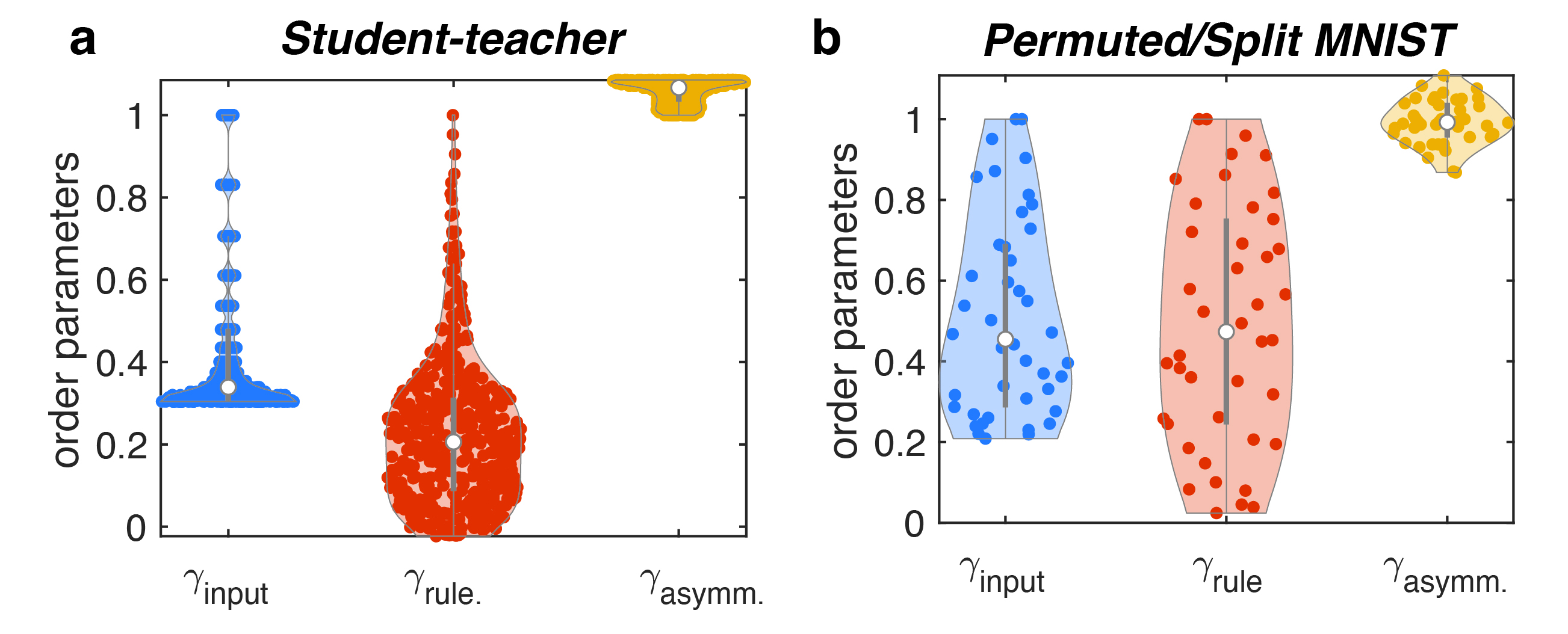
Figure 1: Distribution of the Three OPs.
a Violin plot showing the distribution of $\gamma_{input}$,$\gamma_{rule}$ and $\gamma_{asymm}$ by varying $\rho_{teacher}$ and $\rho_{input}$ in the student-teacher dataset.
b Same as a, but for permuted/split MNIST dataset by varying the permutation ratio (permuted MNIST) or split ratio (split MNIST).
In these examples $\gamma_{input}$ and $\gamma_{rule}$ vary significantly with task similarity, while $\gamma_{asymm}$ remains roughly unchanged.

2.6 Hidden-Layer Kernels and Representational Changes

2.6.1 Hidden-layer kernels

To estimate the hidden-layer kernels, we make an heuristic approximation that the probability distribution of $\Phi(\mathcal{W}_{2}^{\alpha},\bm{x})$, $\Phi(\mathcal{W}_{1},\bm{x})$ induced by the Gaussian prior proportional to $\exp(-S_{0}(\mathcal{W}))$ is also Gaussian with mean 0 and covariances

$$N^{-1}\langle\Phi(\mathcal{W}_{1},\bm{x})\cdot\Phi(\mathcal{W}_{1},\bm{x}^{\prime})\rangle_{\mathcal{W}}=K_{1,1}^{1}(\bm{x},\bm{x}^{\prime})$$ (151)

$$N^{-1}\langle\Phi(\mathcal{W}_{2}^{\alpha},\bm{x})\cdot\Phi(\mathcal{W}_{2}^{\beta},\bm{x}^{\prime})\rangle_{\mathcal{W}}=\begin{cases}K_{2,2}^{1}(\bm{x},\bm{x}^{\prime})&\alpha=\beta\\ K_{2,2}^{0}(\bm{x},\bm{x}^{\prime})&\alpha\neq\beta\end{cases}$$ (152)

$$N^{-1}\langle\Phi(\mathcal{W}_{1},\bm{x})\cdot\Phi(\mathcal{W}_{2}^{\alpha},\bm{x}^{\prime})\rangle=K_{1,2}^{1}(\bm{x},\bm{x}^{\prime})$$ (153)

The approximation is exact for linear networks. This approximation allows us to evaluate second moments in the representations over the posterior distribution in $\Theta$ by evaluating Gaussian integrals.In particular, we define the similarity between representations

$$K_{sim}(\bm{x},\bm{x}^{\prime})\equiv N^{-1}\langle\Phi(\mathcal{W}_{2},\bm{x})\cdot\Phi(\mathcal{W}_{2},\bm{x}^{\prime})\rangle$$ (154)

where the average is w.r.t. the posterior distribution Eq. 3 for $T=2$.We have

$$K_{sim}(\bm{x},\bm{x}^{\prime})=K_{2,2}^{1}(\bm{x},\bm{x}^{\prime})-\frac{1}{N}(u_{1,1}^{1}\bm{k}_{2,1}^{1}(\bm{x})^{\top}\langle\bm{v}_{1}\bm{v}_{1}^{\top}\rangle\bm{k}_{1,2}^{1}(\bm{x}^{\prime})+u_{2,2}^{0}\Delta\bm{k}_{2,2}(\bm{x})^{\top}\langle\bm{v}_{2}\bm{v}_{2}^{\top}\rangle\Delta\bm{k}_{2,2}(\bm{x}^{\prime})\\ +u_{1,2}^{1}\bm{k}_{2,1}^{1}(\bm{x})^{\top}\langle\bm{v}_{1}\bm{v}_{2}^{\top}\rangle\Delta\bm{k}_{2,2}(\bm{x}^{\prime})+u_{1,2}^{1}\Delta\bm{k}_{2,2}(\bm{x})^{\top}\langle\bm{v}_{2}\bm{v}_{1}^{\top}\rangle\bm{k}_{1,2}^{1}(\bm{x}^{\prime})\\ +u_{2,2}^{0}\bm{k}_{2,2}^{0}(\bm{x})^{\top}\langle\delta\bm{v}_{2}\delta\bm{p}_{2}^{\top}\rangle\Delta\bm{k}_{2,2}(\bm{x}^{\prime})+u_{2,2}^{0}\Delta\bm{k}_{2,2}(\bm{x})^{\top}\langle\delta\bm{v}_{2}\delta\bm{p}_{2}^{\top}\rangle\bm{k}_{2,2}^{0}(\bm{x}^{\prime})\\ +\left(u_{2,2}^{1}-u_{2,2}^{0}\right)\left(\bm{k}_{2,2}^{1}(\bm{x})^{\top}\langle\bm{v}_{2}\bm{v}_{2}^{\top}\rangle\bm{k}_{2,2}^{1}(\bm{x}^{\prime})-\bm{k}_{2,2}^{0}(\bm{x})^{\top}\langle\bm{v}_{2}\bm{v}_{2}^{\top}\rangle\bm{k}_{2,2}^{0}(\bm{x}^{\prime})\right))$$ (155)

where the statistics of $\bm{v}_{2},\bm{p}_{2}$ and $\bm{v}_{1}$ are given in Supplementary Eqs. 323329, with $\left\{m_{t,t^{\prime}}^{1}\right\}_{t,t^{\prime}=1,\cdots,T},\left\{m_{t,t^{\prime}}^{0}\right\}_{t,t^{\prime}=1,\cdots,T}$ replaced by $\left\{u_{t,t^{\prime}}^{1}\right\}_{t,t^{\prime}=1,\cdots,T},\left\{u_{t,t^{\prime}}^{0}\right\}_{t,t^{\prime}=1,\cdots,T}$. $K(\bm{x},\bm{x}^{\prime})$ has two contributions, the first term in Supplementary Eq. 155 corresponds to averaging Supplementary Eq. 154 w.r.t. the Gaussian prior in $\mathcal{W}_{2}$, and the rest of the terms are induced by learning, which we denote as $K(\bm{x},\bm{x}^{\prime})$. $K({\bf x},{\bf x}^{\prime})$ thus captures the changes in the similarity matrix before learning (at random Gaussian initialization) and after learning.

Although the learning induced terms are sub-leading and of $\mathcal{O}(1)$, we see in the main text that the structure of these terms can affect the generalization performance. We note that, in the overfitting regime, because $u_{2,2}^{1},u_{2,2}^{0}\sim\mathcal{O}(\lambda^{1/2})$ and $u_{2,2}^{1}-u_{2,2}^{0}\sim\mathcal{O}(\lambda^{-1/2})$, several terms vanish in the large $\lambda$ limit, and we have

$$K_{sim}(\bm{x},\bm{x}^{\prime})=K_{2,2}^{1}(\bm{x},\bm{x}^{\prime})-\frac{1}{N}(u_{1,1}^{1}\bm{k}_{2,1}^{1}(\bm{x})^{\top}\langle\bm{v}_{1}\bm{v}_{1}^{\top}\rangle\bm{k}_{1,2}^{1}(\bm{x}^{\prime})\\ -\left(u_{2,2}^{0}\right)^{2}\Delta\bm{k}_{2,2}(\bm{x})^{\top}\tilde{\bm{K}}_{2,2}^{-1}\bm{K}_{2,2}^{0}\tilde{\bm{K}}_{2,2}^{-1}\Delta\bm{k}_{2,2}(\bm{x}^{\prime})\\ +u_{2,2}^{0}\bm{k}_{2,2}^{0}(\bm{x})^{\top}\tilde{\bm{K}}_{2,2}^{-1}\Delta\bm{k}_{2,2}(\bm{x}^{\prime})+u_{2,2}^{0}\Delta\bm{k}_{2,2}(\bm{x})^{\top}\tilde{\bm{K}}_{2,2}^{-1}\bm{k}_{2,2}^{0}(\bm{x}^{\prime})\\ -\left(u_{2,2}^{1}-u_{2,2}^{0}\right)u_{2,2}^{0}\left(\bm{k}_{2,2}^{1}(\bm{x})^{\top}\tilde{\bm{K}}_{2,2}^{-1}\bm{K}_{2,2}^{0}\tilde{\bm{K}}_{2,2}^{-1}\bm{k}_{2,2}^{1}(\bm{x}^{\prime})-\bm{k}_{2,2}^{0}(\bm{x})^{\top}\tilde{\bm{K}}_{2,2}^{-1}\bm{K}_{2,2}^{0}\tilde{\bm{K}}_{2,2}^{-1}\bm{k}_{2,2}^{0}(\bm{x}^{\prime})\right))$$ (156)

the structure of $K_{sim}(\bm{x},\bm{x}^{\prime})$ is not affected by the labels of the second task $\bm{Y}_{2}$, confirming our observation that the network fails to learn task 2 relevant representations in this regime. In the main text Fig.8, we evaluate the kernel on the training data, $K_{sim}(\bm{X}_{1})=K_{sim}(\bm{X}_{1},\bm{X}_{1})\in\mathbb{R}^{P\times P},K_{sim}(\bm{X}_{2})=K_{sim}(\bm{X}_{2},\bm{X}_{2})\in\mathbb{R}^{P\times P}$, and similarly $K(\bm{X}_{1})=K(\bm{X}_{1},\bm{X}_{1})\in\mathbb{R}^{P\times P},K(\bm{X}_{2})=K(\bm{X}_{2},\bm{X}_{2})\in\mathbb{R}^{P\times P}$.

2.6.2 Representational changes

For the changes in the representation of $\bm{x}$ defined as $\Delta\Phi(\bm{x})=\Phi(\mathcal{W}_{2},\bm{x})-\Phi(\mathcal{W}_{1},\bm{x})$, we can derive the second moments in $\Delta\Phi(\bm{x})$ using the same Gaussian approximation for calculating the hidden-layer kernels. In the $\lambda\rightarrow\infty$ limit, we obtain

$$\Delta\Phi(\bm{x})\cdot\Delta\Phi(\bm{x}^{\prime}) =-u_{2,2}^{0}\Delta\bm{k}_{2,2}(\bm{x})^{\top}\langle\bm{v}_{2}\bm{v}_{2}^{\top}\rangle\Delta\bm{k}_{2,2}(\bm{x}^{\prime})$$ (157)

By analyzing the scalings of $u_{2,2}^{1},u_{2,2}^{0}$,$u_{2,2}^{1}-u_{2,2}^{0}$ and $u_{1,2}^{1}$ in the different regimes in the $\lambda\rightarrow\infty$ limit, we can analyze the behavior of $\Delta\Phi(\bm{x})\cdot\Delta\Phi(\bm{x}^{\prime})$. In the regime $\alpha<1$, we have $\Delta\Phi(\bm{x})\cdot\Delta\Phi(\bm{x}^{\prime})=0$,confirming that the hidden-layer weights do not change from task 1 to task 2. In the overfitting regime, by evaluating $\langle\bm{v}_{2}\bm{v}_{2}^{\top}\rangle$ with the corresponding scaling of the renormalization factors, we have

$$\Delta\Phi(\bm{x})\cdot\Delta\Phi(\bm{x}^{\prime}) =\left(u_{2,2}^{0}\right)^{2}\Delta\bm{k}_{2,2}(\bm{x})^{\top}\tilde{\bm{K}}_{2,2}^{-1}\bm{K}_{2,2}^{0}\tilde{\bm{K}}_{2,2}^{-1}\Delta\bm{k}_{2,2}(\bm{x}^{\prime})$$ (158)

In the generalization regime, we have

$$\Delta\Phi(\bm{x})\cdot\Delta\Phi(\bm{x}^{\prime})$$

$$= \left(u_{2,2}^{0}\right)^{2}\Delta\bm{k}_{2,2}(\bm{x})^{\top}\tilde{\bm{K}}_{2,2}^{-1}\bm{K}_{2,2}^{0}\tilde{\bm{K}}_{2,2}^{-1}\Delta\bm{k}_{2,2}(\bm{x}^{\prime})$$

$$+u_{2,2}^{0}\Delta\bm{k}_{2,2}(\bm{x})^{\top}\tilde{\bm{K}}_{2,2}^{-1}\left(\bm{Y}_{2}-\tilde{\bm{K}}_{2,1}\tilde{\bm{K}}_{1,1}^{-1}\bm{Y}_{1}\right)\left(\bm{Y}_{2}-\tilde{\bm{K}}_{2,1}\tilde{\bm{K}}_{1,1}^{-1}\bm{Y}_{1}\right)^{\top}\tilde{\bm{K}}_{2,2}^{-1}\Delta\bm{k}_{2,2}(\bm{x}^{\prime})$$ (159)

Therefore as long as $\alpha>1$, $\lVert\Delta\Phi(\bm{x})\rVert^{2}\geq 0$. In the overfitting regime the structure of $\Delta\Phi(\bm{x})\cdot\Delta\Phi(\bm{x}^{\prime})$ is not aligned with either $\bm{Y}_{1}$ nor $\bm{Y}_{2}$, and in the generalization regime the structure is affected by both $\bm{Y}_{1}$ and $\bm{Y}_{2}$. While the result holds for general $\bm{x}$, in the main text we only mentioned the norm of representational changes on $\bm{X}_{1}$ and their alignment with $\bm{Y}_{1}$ (Supplementary Note 5), as they are directly related to forgetting on task 1 ($F_{2,1}$).

3 Asymmetric OP in Multi-Head CL

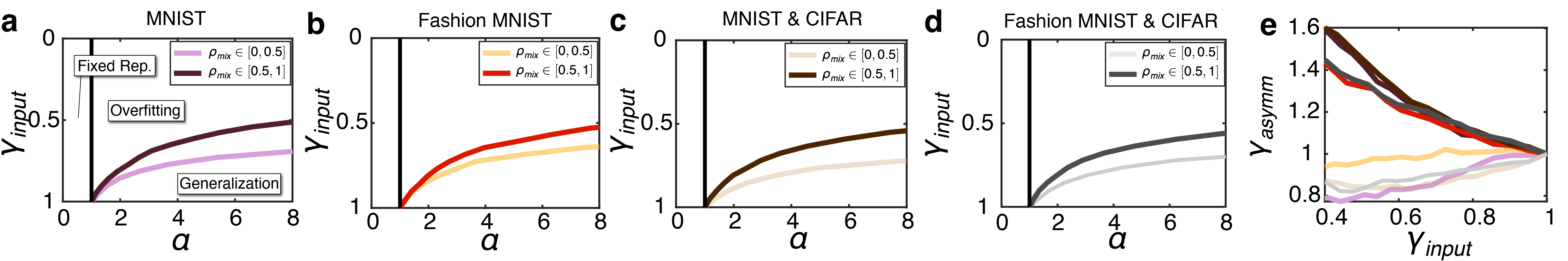
Figure 2: Effect of Ordering on the Asymmetric OP and Phase-Transition Boundaries.
a Phase-transition boundaries in the 2D $\gamma_{input}-\alpha$ plane on the MNIST dataset. $\gamma_{input},\gamma_{rule},\gamma_{asymm}$ are simultaneously varied as $\rho_{mix}$ is varied. There is a larger generalization regime when $\rho_{mix}$ varies from 1 to 0.5, compared to $\rho_{mix}$ varying from 0 to 0.5, exhibiting an ordering effect on the phase-transition boundary.
b Same as a but on Fashion MNIST.
c Same as a, first dataset is MNIST, second dataset is CIFAR 10, both with binary labels of even vs. odd classification.
d Same as c, but replacing the first dataset with Fashion MNIST.
e $\gamma_{asymm}$ as a function of $\gamma_{input}$ as $\rho_{mix}$ is varied on the 4 examples in a-d, shown with corresponding colors. $\gamma_{asymm}$ is different when the ordering of the two tasks is switched, in the examples we show varying $\rho_{mix}$ from 1 to 0.5 corresponds to larger $\gamma_{asymm}$ compared to varying $\rho_{mix}$ from 0 to 0.5 by flipping the order of the two tasks.

In Supplementary Note 2.5, we derived the phase-transition boundaries separating the 3 different regimes, which depends on task relations through 3 order parameters. On examples of split, permuted MNIST and the student-teacher dataset, one of the OPs ($\gamma_{asymm}$) remains unchanged (Supplementary Fig. 2), this is due to the symmetric nature of the tasks themselves.

We also find examples where $\gamma_{asymm}$ significantly varies with task similarity, and affect the position of the phase-transition boundary, particularly when the two tasks are largely different in their statistics. Unlike $\gamma_{input}$ and $\gamma_{rule}$, $\gamma_{asymm}$ is asymmetric in the ordering of task 1 and task 2, revealing the ordering effect on learning. In Supplementary Fig. 2 we show 4 example tasks where $\gamma_{asymm}$ varies significantly, resulting in different phase-transition boundaries by switching the order of the two tasks.

In all examples we smoothly vary task relations by adjusting the split ratio of two datasets, as in Method 6. The first task is composed of $1-x\%$ of the first dataset, and $x\%$ of the second dataset, and vice versa for the second task. Therefore at $x\%=50\%$ the two tasks are identical. Furthermore, changing the split ratio from $x\%$ to $1-x\%$ results in flipping the order of the two tasks. In Supplementary Fig. 2a, the first dataset is composed of 0 and 1 digits in MNIST, with binary labels of 0 vs. 1. The second dataset is composed of all 10 digits in MNIST, with binary labels of even vs. odd. We show the phase-transition boundaries as we vary $x\%$ from $0\%$ to $50\%$, and from $100\%$ to $50\%$ (by reversing the order of the two tasks). We observe a larger generalization regime when we vary $x\%$ from $100\%$ to 50%. In Supplementary Fig. 2b, we show similar results as in Supplementary Fig. 2a, but on the Fashion MNIST dataset.

In Supplementary Fig. 2 c, d we evaluate tasks composed of two different source datasets. In Supplementary Fig. 2 c, the first dataset is MNIST, and the second dataset is CIFAR 10, both with binary labels of even vs. odd. We observe a similar phenomenon as in Supplementary Fig. 2a,b, where the generalization regime becomes larger if we vary $x\%$ from 100% to 50%. Similar result is obtained when we change the first dataset to Fashion MNIST (Supplementary Fig. 2 d).

In Supplementary Fig. 2 e, we show $\gamma_{asymm}$ as a function of $\gamma_{input}$, as we vary $x\%$, for the 4 pairs of tasks. We observe that in all cases, as we vary $x\%$ from 0% to 50%, $\gamma_{asymm}$ gradually increases to 1 (light colors in Supplementary Fig. 2e, colors correspond to different datasets shown in a-d). By flipping the order of the two tasks and vary $x\%$ from $100\%$ to $50\%$, the value of $\gamma_{asymm}$ is significantly larger (dark colors in Supplementary Fig. 2e), and gradually decreases to 1. A larger $\gamma_{asymm}$ corresponds to a larger generalization regime.

Interestingly, in these 4 pairs of examples we evaluated, we observe that a larger $\gamma_{asymm}$ usually correspond to learning a more difficult task first, and proceeding to learn an easier task (e.g., CIFAR 10 is intuitively perceived as a more difficult task than both MNIST and Fashion MNIST; and even vs odd classification is generally considered a more difficult task than 0 vs. 1 classification), and thus learning a more difficult task first increases the generalization regime and mitigates anterograde interference. This observation indicates that $\gamma_{asymm}$ may serve as an OP measuring the relative difficulty of a pair of tasks, and has interesting implications on curriculum learning.

4 Order Parameters and Short-Term Forgetting in Single-Head CL.

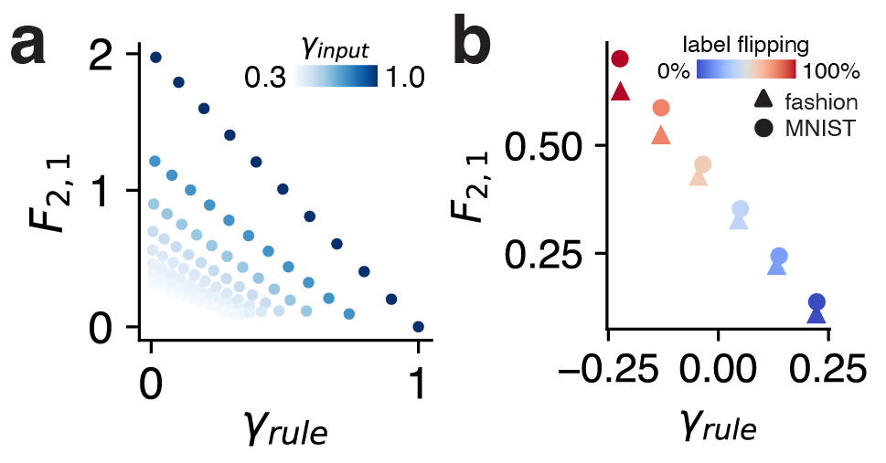
Figure 3: Order Parameters and Short-Term Forgetting in Single-Head CL.
a Short-term forgetting, defined as the training loss of task 1 after learning two student-teacher tasks ($F_{2,1}$). Each point corresponds to a different $\rho_{input},\rho_{teacher}$ combination used for task generation (Methods). For a fixed level of $\gamma_{input}$, forgetting decreases approximately linearly in $\gamma_{rule}$. Forgetting is smaller with lower $\gamma_{input}$ or higher $\gamma_{rule}$.
b $F_{2,1}$ as a function of $\gamma_{rule}$ in label-flipping tasks (Methods). Task sequences made with different levels of label flipping differ only in $\gamma_{rule}$. $F_{2,1}$ also decreases approximately linearly in $\gamma_{rule}$.

5 Phase Transition in the Structure of Representational Changes in Multi-Head CL

In multi-head CL, since we keep $\bm{a}^{{\rm task}\ 1}$ intact when learning the second task, the behavior of forgetting on the first task ($F_{2,1}$) must be accounted for by the behavior of the change in the representations ($\Delta\Phi({\bf X}_{1})$). In Fig.6, we showed that there’s an abrupt transition in $F_{2,1}$ ,which cannot be explained by the behavior of the magnitude of the representational changes, $P^{-1}\lVert\Delta\Phi({\bf X}_{1})\rVert^{2}$. Therefore, the transition must be accounted for by abrupt changes in the structure of $\Delta\Phi({\bf X}_{1})$. In this section, we further investigated the structure of representational changes. Motivated by recent results showing that the representations become aligned to task labels after learning one task [42, 63, 41], we focused on how much $\Delta\Phi({\bf X}_{1})$ is aligned with labels of the first task ${\bf Y}_{1}$,measured by the alignment metric

$$A({\bf X}_{1})\equiv\frac{{\bf Y}_{1}^{\top}\Delta\Phi({\bf X}_{1})\Delta\Phi({\bf X}_{1})^{\top}{\bf Y}_{1}}{\left\|\Delta\Phi({\bf X}_{1})\right\|^{2}\cdot\lVert{\bf Y}_{1}\rVert^{2}}.$$ (160)

First, we show $A(\bm{X}_{1})$ on the student-teacher task, as a function of $\rho_{teacher}(\rho_{input})$ and $\alpha$(Supplementary Fig. 4) The analysis reveals that $A({\bf X}_{1})$ undergoes a similar phase transition from the overfitting to the generalization regime as $F_{2,1}$ and $G_{2,2}$ do. $A({\bf X}_{1})=0$ in the overfitting regime, suggesting that although the magnitude of representational changes is non-zero, the direction of the change is orthogonal to ${\bf Y}_{1}$. Therefore, the changes do not result in losing task 1 relevant information, and does not affect the network output, leading to $F_{2,1}=0$. In contrary, $A({\bf X}_{1})$ becomes non-zero in the generalization regime as the representational changes become aligned with ${\bf Y}_{1}$, resulting in nonzero $F_{2,1}$.

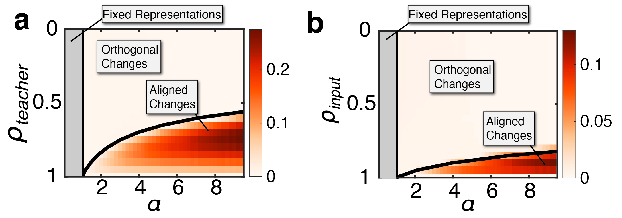
Figure 4: Phase Transition in the Alignment Metric in the Student-Teacher Task.
a Phase transition of $A({\bf X}_{1})$ in the $\rho_{teacher}-\alpha$ plane, for student-teacher tasks ($\rho_{input}$ is fixed at $1$). The alignment metric exhibits the same 3 regimes as $F_{2,1}$ and $G_{2,2}$ with the same phase-transition boundaries.
b Same as a, but for fixed $\rho_{teacher}=1$ and different $\rho_{input}$.

We then show that similar to the phase transition in $F_{2,1}$ and $G_{2,2}$, the phase transition in $A(\bm{X}_{1})$ also happens in general data. The phase-transition boundary occurs at the same $\alpha_{c}(\gamma_{input},\gamma_{rule})$ as $F_{2,1}$ and $G_{2,2}$ (as shown by comparing Fig. 7 and Supplementary Fig. 5). $A(\bm{X}_{1})=0$ for $1<\alpha<\alpha_{c}$, and $A(\bm{X}_{1})>0$ for $\alpha>\alpha_{c}.$as

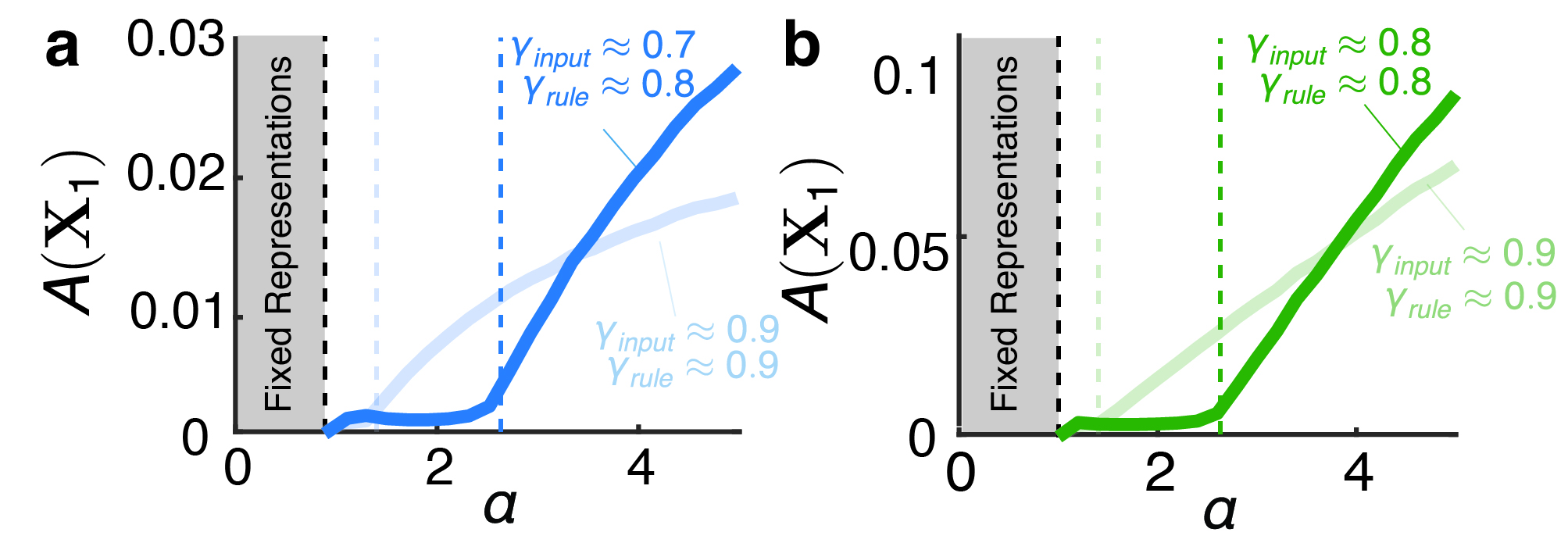
Figure 5: Phase Transition in the Alignment Metric in Benchmark Datasets.
a $A({\bf X}_{1})$ as a function of $\alpha$ for the same tasks and parameters as in Fig. 7a. $A(\bm{X}_{1})=0$ when $1<\alpha<\alpha_{c}$, $A(\bm{X}_{1})>0$ when $\alpha>\alpha_{c}$.Black dash line: $\alpha=1$. Colored dashed line: theoretical prediction of $\alpha_{c}$.
b Same as a, but for the same task and parameters as in Fig. 7b.

5.1 Phase Transitions in Gradient Descent Simulations in Multi-Head CL

In multi-head CL, we observe surprising phenomenon of phase transition in our theory, suggesting that the performance of the network changes abruptly, dependent on task similarity and the network width ($\alpha$). In this section, we present numerical results validating our theoretical analysis.

To capture multi-head CL behaviors in the $\lambda\rightarrow\infty$ limit, we first train an NN with GD on the first task until the network reaches zero training error. We add an explicit regularizer penalizing the change in hidden-layer weights as we proceed to learn the next tasks. The GD dynamics is given by

$$\mathcal{W}_{t}^{\tau}=\mathcal{W}_{t}^{\tau-1}-\eta\nabla_{\mathcal{W}_{t}^{\tau-1}}\mathcal{L}(f_{t}^{t}(\Theta_{t}^{\tau-1}),D_{t})-\eta\gamma(\mathcal{W}_{t}^{\tau-1}-\mathcal{W}_{t-1})$$ (161)

$$a_{t}^{\tau}=a_{t}^{\tau-1}-\eta\nabla_{a_{t}^{\tau-1}}\mathcal{L}(f_{t}^{t}(\Theta_{t}^{\tau-1}),D_{t})$$ (162)

here we use $t$ to denote the index of the task, and $\tau$ to denote the time steps during training. For each task, the readout weights are always initialized as $a_{t}^{0}\sim\mathcal{N}(0,\sigma_{0}^{2})$, where as the hidden-layer weights $\mathcal{W}_{t}^{0}$ are initialized as $\mathcal{W}_{t-1}$, which denotes the weights obtained at the end of training on the previous task. Except for on the first task, $\mathcal{W}_{1}^{0}$ is initialized as $\mathcal{W}_{1}^{0}\sim\mathcal{N}(0,\sigma_{0}^{2})$.

The learning process is run sufficiently long, in order to approximate the $\lambda\rightarrow\infty$ limit where the closest solution to $\mathcal{W}_{t-1}$ is obtained.While our theory depicts the statistics over the posterior weights, and do not directly correspond to NNs trained with GD dynamics, it makes qualitative accurate prediction of the existence of the 3 different regimes. Furthermore, as shown in Supplementary Fig. 6 top panels, on both split (a) and permuted MNIST(b), the theoretical phase-transition boundary (black lines) accurately predicts the position of phase transition in GD simulations.

Although our theory has not been extended to $L>1$, we conduct GD simulations on deeper networks with $L=2$, as shown in Supplementary Fig. 6 bottom panels. The dependence of $F_{2,1}$ and $G_{2,2}$ on task similarity and $\alpha$ are similar as in $L=1$. However, the regime where $F_{2,1}$ is essentially 0 and $G_{2,2}$ is very large (corresponding to the overfitting regime) becomes larger. This suggests that adding more layers mitigates forgetting, while increasing the anterograde interference effect. Extending the current theory to networks with more than 1 hidden layer is an ongoing challenging direction.

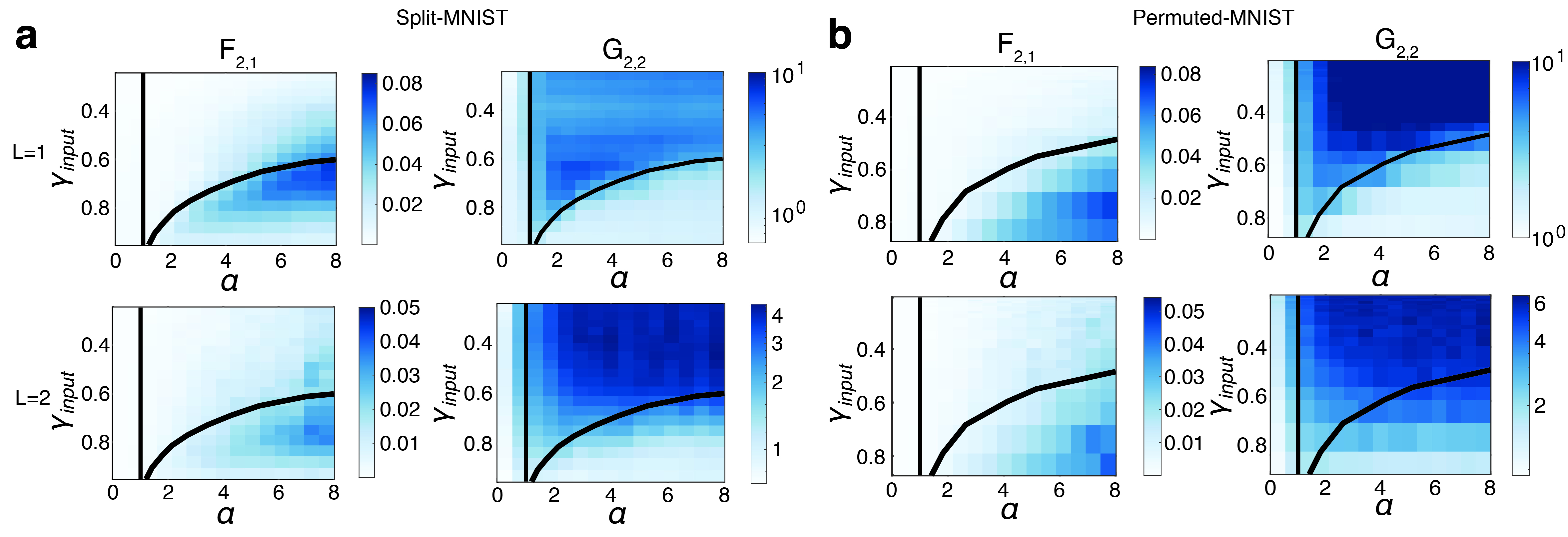
Figure 6: Phase Transition in Networks Trained with Gradient Descent and Explicit Regularizer.
a $F_{2,1}$ (left) and $G_{2,2}$(right) evaluated from networks trained with GD and an explicit regularizer (Supplementary Eqs. 162, 161), as a function of $\gamma_{input}$ and $\alpha$ for split MNIST, for $L=1$(top) and $L=2$(bottom). The same 3 regimes are observed as predicted by the theory. In networks with $L=1$, theoretical approximation of the phase-transition boundary (black line) accurately matches the simulation.In networks with $L=2$, the overfitting regime extends beyond the theoretical phase-transition boundary of $L=1$ (black line), indicating a stronger anterograde interference effect.Simulations are done with $\gamma=0.1$,$\sigma_{0}=1$, $\eta=0.01$ for $L=1$ and $\eta=0.001$ for $L=2$.
b Same as a, for permuted MNIST task. Simulations are done with $\gamma=0.1$,$\sigma_{0}=1,$$\eta=0.005$ for $L=1$ and $\eta=0.001$ for $L=2$.
The tasks are identical as those shown in Fig. 7.

6 Performance and Representations at Finite $\lambda$ in Multi-Head CL

6.1 Phase Diagram at Finite $\lambda$

In the main text we investigated the phase transitions in multi-head CL when $\lambda\rightarrow\infty$. To check whether the phase diagrams provide insights for qualitative behaviors of $F_{2,1}$ and $G_{2,2}$ at finite $\lambda$, here we show the 2-D phase diagram in the $\gamma_{input}-\alpha$ space for split and permuted MNIST at finite but relatively large $\lambda$ ($\lambda=10$). Interestingly, as shown in Supplementary Fig.7, we found that although the phase transitions disappear as expected, some qualitative behaviors of $F_{2,1}$ and $G_{2,2}$ still persists. For example, $F_{2,1}$ increases with $\alpha$, suggesting that there’s more forgetting when the load increases. $F_{2,1}$ can also be non-monotonic in task similarities for a range of $\alpha$. $G_{2,2}$ is large when the tasks are dissimilar, and decreases with $\gamma_{input}$ . These common qualitatively behaviors are also present in the $\lambda\rightarrow\infty$ limit, and suggest that our analytical results on the phase transitions at $\lambda\rightarrow\infty$ provide qualitative insights on how the network performance depends on $\alpha$ and task relations for a wide range of finite $\lambda$.

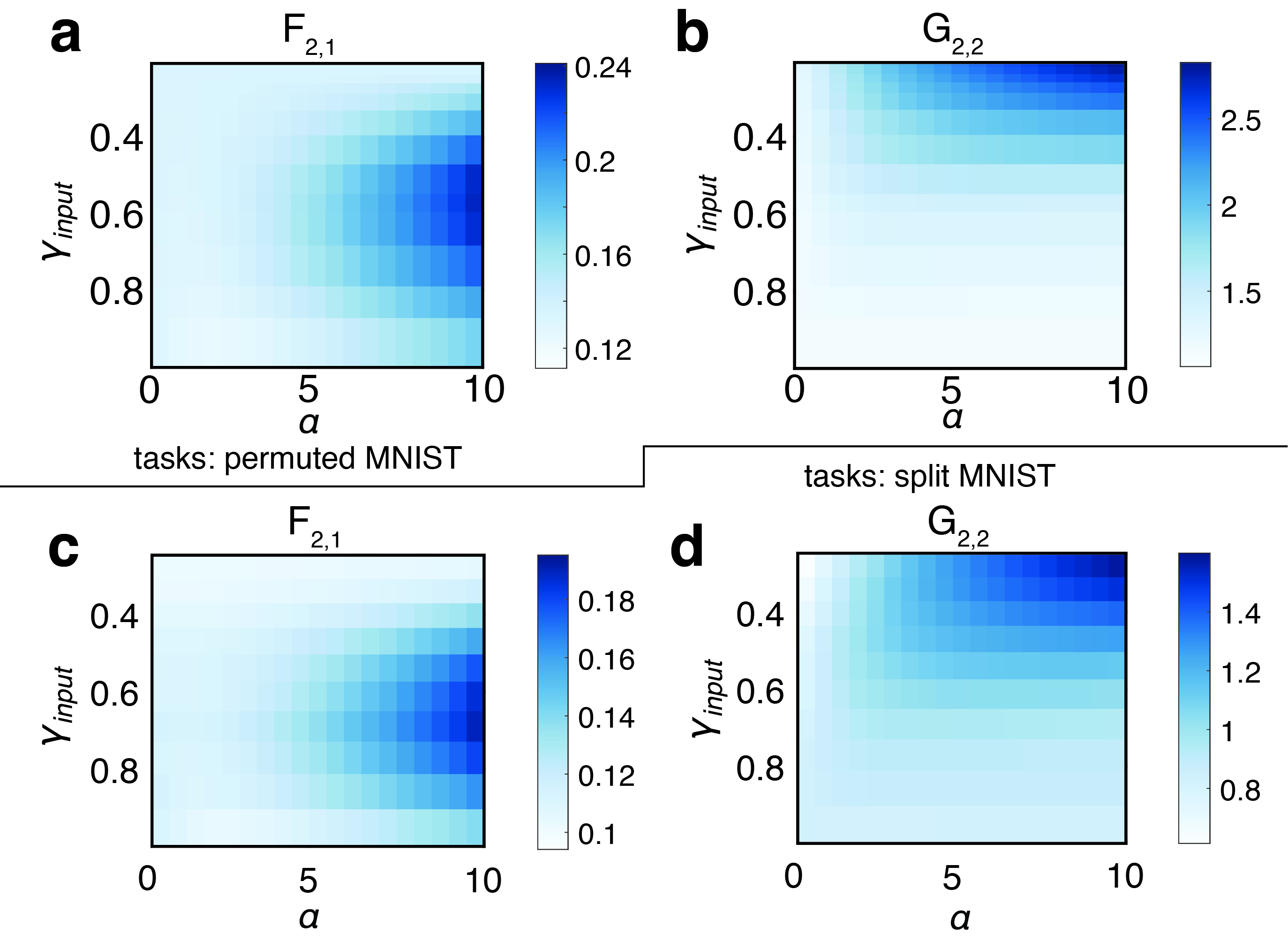
Figure 7: Phase Diagrams for Permuted MNIST and Split MNIST at Finite $\lambda$.
a, b $F_{2,1}$ and $G_{2,2}$ as a function of $\alpha$ and $\gamma_{input}$ for permuted MNIST at $\lambda=10$. There is no abrupt phase transitions as shown in Fig.7 as both $F_{2,1}$ and $G_{2,2}$ vary smoothly, but the dependence on $\alpha$ and $\gamma_{input}$ is qualitatively similar to the $\lambda\rightarrow\infty$ limit.
c, d Same as a, b, but for the split MNIST dataset.

6.2 Dependence of Optimal Regularization Strengths on $\alpha$ and Task Relations

For multi-head CL, we showed that there’s an optimal finite $\lambda$ which can avoid the overfitting regime at the cost of slightly increasing forgetting, achieving a balance between retrograde and anterograde interference by minimizing $max(G_{2,1},G_{2,2})$. Here we show a more thorough analysis on the effect of $\lambda$ at different values of $\alpha$ and for different task relations. As shown in Supplementary Fig. 8, the optimal finite $\lambda$ exists for almost all values of $\alpha$ and $\gamma_{input}$, on both split and permuted MNIST tasks. Furthermore, the magnitude of the optimal $\lambda$ is not significantly affected by either $\alpha$ or task relations, and remains in the range of $1-10$ for all combinations of $\alpha$ and $\gamma_{input}$.

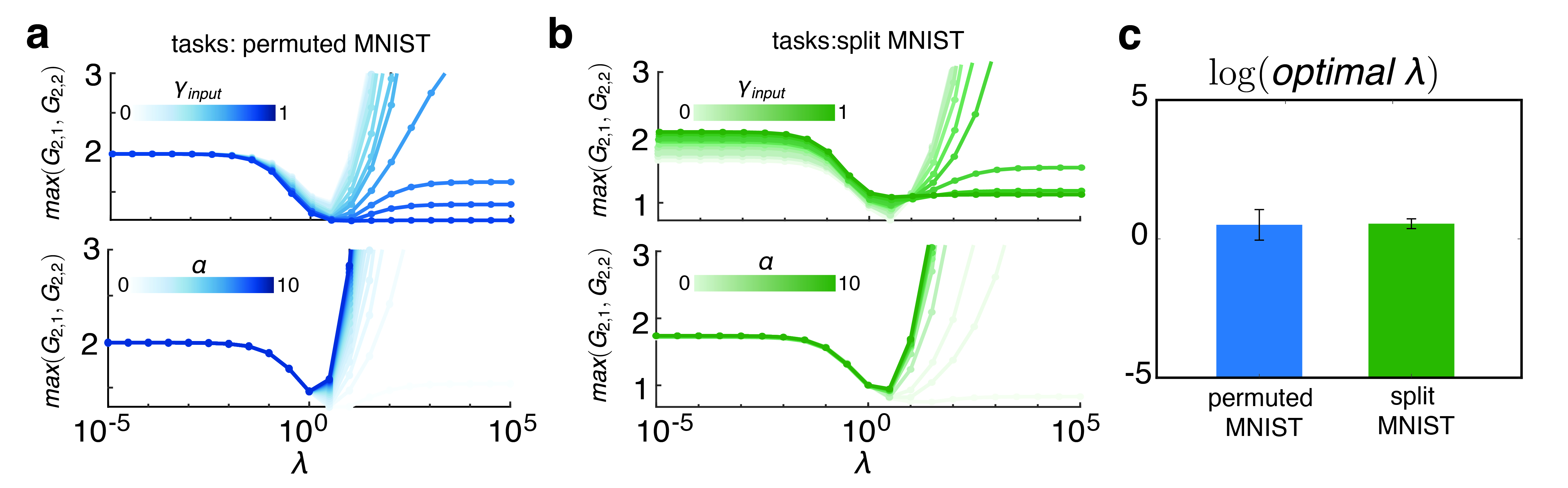
Figure 8: Optimal Regularization Strengths for Permuted MNIST and Split MNIST is Independent of $\alpha$ and Task Relations.
a $\max(G_{2,1},G_{2,2})$ as a function of $\lambda$ for permuted MNIST. For a fixed $\alpha$ ($\alpha=3$) and a wide range of $\gamma_{input}$ (top); or for a fixed pair of tasks (full permutation, $\gamma_{input}\approx 0.2$) and a wide range of $\alpha$ (bottom). There exists an optimal finite $\lambda$ that minimizes $\max(G_{2,1},G_{2,2})$ for a wide range of $\gamma_{input}$ and $\alpha$.
b Same as a, but for the split MNIST dataset.
c The average $\log(\text{optimal}\ \lambda)$ for permuted and split MNIST, errorbars are standard deviations across all combinations of $\alpha$ and $\gamma_{input}$. The order of magnitude of the optimal $\lambda$ does not vary significantly with either $\alpha$ or task relations, and remains roughly order 1.

6.3 Dependence of Kernel Alignment on the Regularization Strength in Multi-Head CL

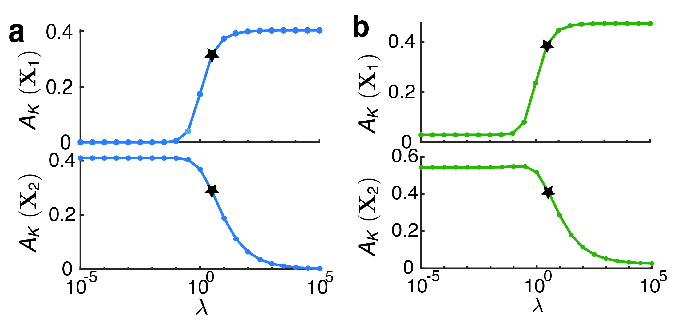
Figure 9: Dependence of the Kernel-Alignment Metric on $\lambda$
a $A_{K^{*}}({\bf X}_{1})$ and $A_{K^{*}}({\bf X}_{2})$ as a function of $\lambda$ for the same tasks and parameters as in Fig. 8a-c. Task 1 alignment monotonically increases with $\lambda$, while task 2 alignment monotonically decreases with $\lambda$. The star indicates the optimal $\lambda$ corresponding to the stars in Fig. 8 a-c.
b Same as a, but for the same task and parameters as in Fig. 8d-f.

In Fig. 8c,f we show examples of the hidden-layer kernels $K^{*}({\bf X}_{1})$ and $K^{*}({\bf X}_{2})$ at different levels of $\lambda$, emphasizing that the network learns shared representations for both tasks at optimal intermediate $\lambda$. To quantify the $\lambda$ dependence of learned representations, we define scalar quantities $A_{K^{*}}({\bf X}_{1})$ and $A_{K^{*}}({\bf X}_{2})$ that measure the alignment between $K^{*}({\bf X}_{1})$,$K^{*}({\bf X}_{2})$ and their corresponding task labels ${\bf Y}_{1}$ and ${\bf Y}_{2}$ (Fig. 8). The alignment metric is defined similarly as in Supplementary Eq. 160. Given by

$$A_{K^{*}}({\bf X}_{t})\equiv\frac{\bm{Y}_{t}^{\top}K^{*}(\bm{X}_{t})\bm{Y}_{t}}{\lVert\bm{Y}_{t}\rVert^{2}\mathrm{Tr}(\sqrt{K^{*}(\bm{X}_{1})^{\top}K^{*}(\bm{X}_{1})})};t\in\left\{1,2\right\}$$ (163)

Confirming the qualitative observations in Fig.8, $A_{K^{*}}({\bf X}_{1})$ monotonically increases with $\lambda$, and $A_{K^{*}}({\bf X}_{2})$ monotonically decreases with $\lambda$. As $\lambda$ increases, the representation becomes more aligned with task 1 and less aligned with task 2. At the optimal $\lambda$ (indicated by black stars), both $A_{K^{*}}({\bf X}_{1})$ and $A_{K^{*}}({\bf X}_{2})$ are relatively large, again indicating a shared representation.

7 Empirical comparison between single-head and multi-head CL

In this work, we focused on single-head CL in the infinite-width limit where $\alpha=0$, and $\sigma$ is small such that the contribution from the mapping variance is neglected. As discussed in the main text, it is trivial that multi-head CL will perform better in this limit, as both anterograde effects and forgetting will be small. However, multi-head CL exhibit catastrophic overfitting, resulting in strong anterograde interference when $\alpha>1$, and the tasks are dissimilar. This suggests that when we take into account the effect of variance, and consider finite $\alpha$, there could be regimes where single-head CL outperforms multi-head CL. We empirically verified this by looking at the generalization performance obtained from training with GD dynamics with explicit regularizers. For multi-head CL, we run the dynamics as described in Supplementary Note 5.1. For single-head CL, the dynamics of $\mathcal{W}_{t}^{\tau}$ is the same as Supplementary Eq. 161, the dynamics of $a_{t}^{\tau}$ is modified as

$$a_{t}^{\tau}=a_{t}^{\tau-1}-\eta\nabla_{a_{t}^{\tau-1}}\mathcal{L}(f_{t}(\Theta_{t}^{\tau-1}),D_{t})-\eta\gamma(a_{t}^{\tau-1}-a_{t-1})$$ (164)

On the first task, $a_{1}^{0}$ is initialized as $\mathcal{N}(0,\sigma_{0}^{2})$. On the following tasks, $a_{t}^{0}$ initializes at $a_{t-1}$ which denotes the weights at the end of training on task $t-1$.

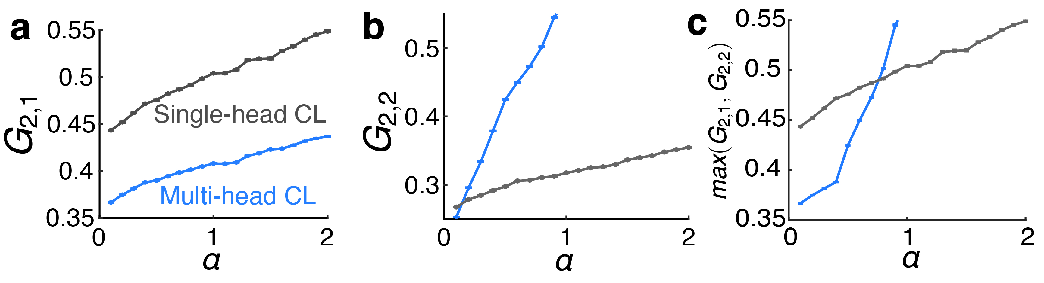
Figure 10: Empirical Comparison Between Single-Head and Multi-Head CL.
a Generalization error on the first task after sequentially learning two tasks for single ($G_{2,1}=\left\langle\mathcal{L}(f_{2},D_{1}^{test})\right\rangle$) and multi-head ($G_{2,1}=\left\langle\mathcal{L}(f_{2}^{1},D_{1}^{test})\right\rangle$) CL as a function of $\alpha$ ($\alpha$ is changed through modifying $N$ and fixing $P$). Multi-head CL always outperforms single-head CL for the entire range of $\alpha$.
b Generalization error on the second task after sequentially learning two tasks for single ($G_{2,2}=\left\langle\mathcal{L}(f_{2},D_{2}^{test})\right\rangle$) and multi-head ($G_{2,2}=\left\langle\mathcal{L}(f_{2}^{2},D_{2}^{test})\right\rangle$) CL as a function of $\alpha$. Both performance worsen with increasing $\alpha$, the generalization error increases at a much faster rate for multi-head CL compared to single-head CL, and starts diverging at $\alpha=1$ as the network enters the overfitting regime. Multi-head CL only outperforms single-head CL when $\alpha$ is very small.
c Same as a, b, but taking the maximum over $G_{2,1}$ and $G_{2,2}$.
Numerics are done using split MNIST dataset with 100% split (Method 6), such that multi-head CL lies in the overfitting regime as long as $\alpha>1$. Detailed parameters are $P=600,\text{$\gamma=0.1,\eta=0.005$}$and $\sigma_{0}=0.5$ for both scenarios.

As shown in Supplementary Fig. 10, for split MNIST task, as we varied the network width, generalization performance on both tasks worsens with decreasing width (or increasing $\alpha$), consistent with previous work which shows that width is beneficial for mitigating forgetting in CL. Multi-head CL always outperforms single-head CL on the first task (Supplementary Fig. 10a), due to the small (or essentially 0) forgetting in multi-head CL in this regime. However, single-head CL almost always outperforms multi-head CL on the second task, except for when $\alpha$ is very close to 0 (Supplementary Fig. 10b). This is due to the divergence of $G_{2,2}$ in the overfitting regime in multi-head CL. Our goal is to keep both generalization errors small, thus to measure the overall performance on both tasks, we use the worst case performance defined by $\max(G_{2,1},G_{2,2})$, as in Fig. 8. Our preliminary results show that for a good overall performance on both tasks, one should choose multi-head CL when $\alpha$ is small, and single-head CL when $\alpha$ becomes large (Supplementary Fig. 10c). It would be an interesting future direction to develop a theory for single-head CL at finite $\alpha$ for more systematic comparison between the two scenarios.

8 Mitigating Anterograde Interference With Intermediate Datasets

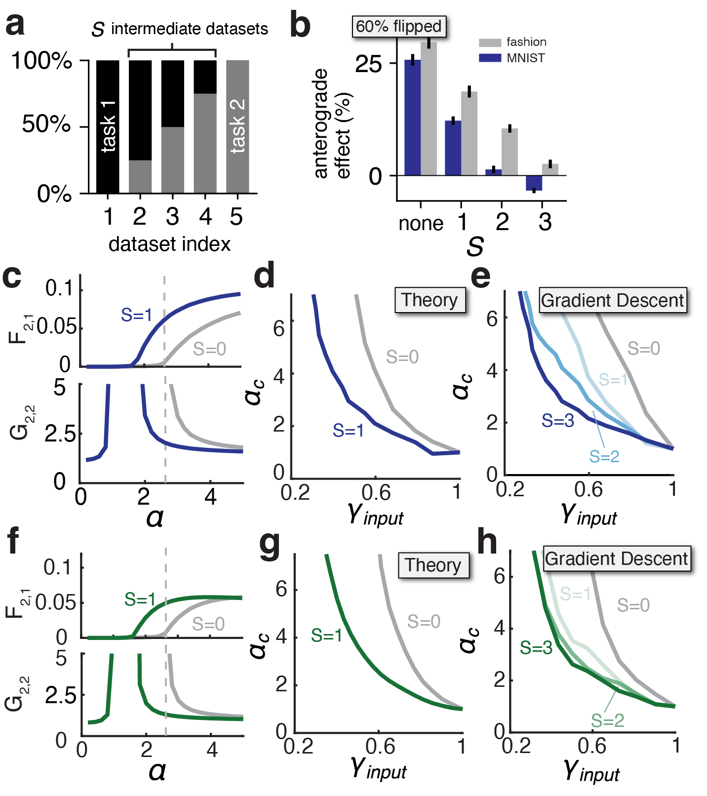
Figure 11: Intermediate Datasets Help Avoid Anterograde Interference.
a Schematics of a task sequence with intermediate datasets. Examples from all datasets represent two tasks with different ratios. The first and last datasets solely contain examples from the first and second tasks, respectively, whereas the $S$ intermediate ones contain a mixture of examples from two tasks. The fraction of examples coming from task 2 increases in later intermediate datasets.
b The anterograde effect of learning task 1 on generalization of task 2 during single-head CL, as a function of the number of intermediate datasets ($S$). In the example here $60\%$ of the labels are flipped.
c The rest of this figure concerns multi-head CL. For a fixed pair of tasks of partially permuted MNIST, forgetting on the first task ($F_{2,1}$) and generalization error on the second task ($G_{2,2}$) as a function of the network load $\alpha=P/N$ without intermediate datasets ($S=0$, gray) and with one intermediate dataset ($S=1$, blue). In both cases there exists a critical $\alpha_{c}$, for $\alpha>\alpha_{c}$ the network is in the generalization regime, $F_{2,1}$ is nonzero, and $G_{2,2}$ is finite; for $1\leq\alpha\leq\alpha_{c}$, the network is in the overfitting regime, $F_{2,1}=0$ and $G_{2,2}$ diverges. The critical $\alpha_{c}$ becomes smaller with the addition of an intermediate dataset, indicating a smaller overfitting regime and mitigated anterograde interference. Dashed line: theoretical prediction of $\alpha_{c}$ for $S=0$.
d The critical $\alpha_{c}$ given by the theory, as a function of $\gamma_{input}$ between task 1 and task 2 in permuted MNIST, without any intermediate datasets ($S=0$, $\alpha_{c}$ calculated by theoretically analyzing the phase-transition boundary and solving Methods Eqs. $\ref{eq:ptboundary},\text{ \ref{eq:u11-1}}$) and with 1 intermediate dataset ($S=$1, $\alpha_{c}$ calculated by estimating the position where $G_{2,2}$ starts to diverge). The difference between the two lines $S=0$ and $S=1$ is larger for small $\gamma_{input}$, indicating that the benefit of intermediate datasets is more significant when task 1 and task 2 are less similar.
e $\alpha_{c}$ evaluated from the phase diagram given by gradient-descent simulation (see text), as a function of $\gamma_{input}$ between task 1 and task 2 in permuted MNIST, without any intermediate datasets ($S=0$) or with 1-3 intermediate datasets ($S=1,2,3$) Increasing $S$ beyond 1 further reduces $\alpha_{c}$.
f-h Same as c-e, but for split MNIST.

We investigated how to reduce interference when sequentially learning incongruent tasks and hypothesized that having “blurry” task boundaries [67] may help. In this case, the NN sequentially learns $S+2$ datasets that contain different mixtures of examples from two tasks (Supplementary Fig. 11a), mimicking real-world settings where the task rule gradually changes over time. The first and last datasets are composed entirely of examples from the first and second tasks, respectively, whereas the $S$ intermediate ones contain mixtures of examples that interpolate between the two extremes.

We first tested the effect of this approach on single-head CL of two label-flipping tasks (Supplementary Fig. 11). The addition of just one intermediate dataset can already alleviate anterograde interference, and stronger benefits are seen with more intermediate datasets.

We next studied whether introducing intermediate tasks between dissimilar tasks can help multi-head CL avoid catastrophic anterograde interference in the overfitting regime. We tested this approach with permuted MNIST and split MNIST and introduced $S$ intermediate datasets between a pair of tasks with given $\gamma_{input},\gamma_{rule}$. For a pair of partially permuted MNIST tasks, we computed $F_{2,1}$ and $G_{2,2}$ as a function of $\alpha$ with $S=1$ (Supplementary Fig. 11c, blue) and $S=0$ (gray). Having blurry task boundaries does not erase the phase transition between the overfitting regime and the generalization regime. However, adding just one intermediate dataset significantly reduces $\alpha_{c}$, resulting in a smaller overfitting regime.

In Supplementary Fig. 11d, we varied $\gamma_{input},\gamma_{rule}$ together by changing the permutation ratio, and plotted $\alpha_{c}$ as a function of $\gamma_{input}$ for $S=0$ and $S=1$ (see Supplementary Note 2.3 and 2.5). We observed that for a wide range of $\gamma_{input}$, task interpolation significantly reduces $\alpha_{c}$, and thus mitigates anterograde interference. Although our theoretical results are so far limited to $S\leq 1$(Supplementary Note 2.3), gradient-descent simulations (Supplementary Fig. 11e) confirmed that introducing intermediate datasets reduces $\alpha_{c}$ even beyond $S=1$.

$\alpha_{c}$ for both gradient descent numerics (Supplementary Fig. 11) and for the theoretical evaluation of $S=1$ (using the mapping statistics in Supplementary Eqs. 113, 114, Supplementary Fig. 11d) are evaluated from 2-D heatmaps of $G_{2,2}$ in the $\gamma_{input}-\alpha$ space, as shown in Supplementary Fig.12 top, using

$$G_{2,2}(\alpha_{c})=\frac{1}{2}(\max_{\alpha>1}G_{2,2}(\alpha)+\min_{\alpha>1}G_{2,2}(\alpha)))$$ (165)

Thus $\alpha_{c}$ is estimated as where $G_{2,2}$ assumes the mid point value of its maximum and minimum. In Supplementary Fig. 12, the evaluated $\alpha_{c}$ is shown by the black lines, accurately capturing the transition in the phase diagram.

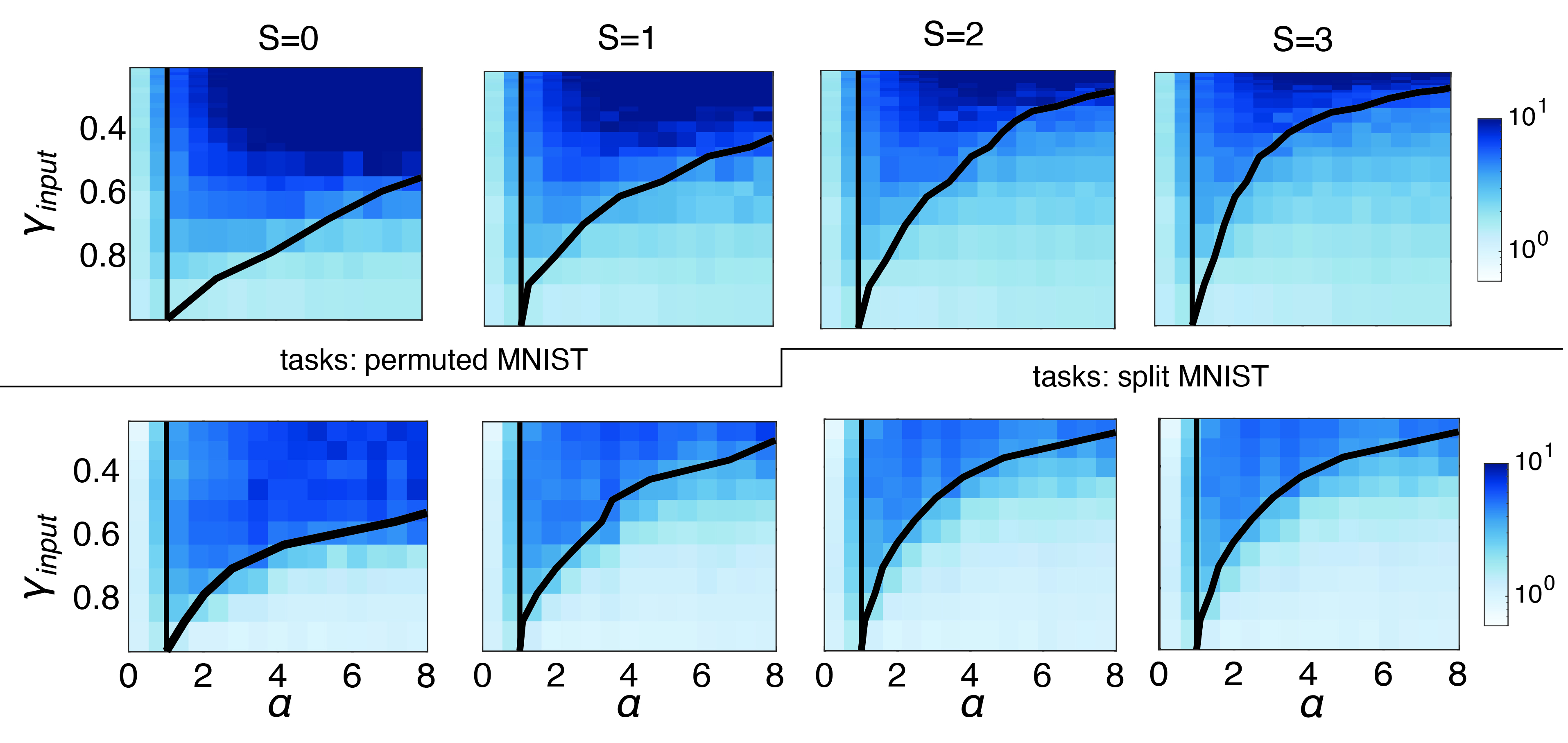
Figure 12: Effect of Task Interpolation in Networks Trained with Gradient Descent and Explicit Regularizer.
$G_{2,2}$ evaluated from networks trained with GD and an explicit regularizer, as a function of $\gamma_{input}$ and $\alpha$, for permuted (top panels) and split (bottom panels) MNIST datasets, from $S=0$ to $S=3$. Black lines show $\alpha_{c}$ estimated using Supplementary Eq. 165.
The tasks are identical as those shown in Fig. 11, $\alpha_{c}$ as shown in Fig. 11e, h correspond to the black lines in this figure. Simulations are done with $\gamma=0.1$,$\sigma_{0}=1$, $\eta=0.01$ for split MNIST, and $\eta=0.005$ for permuted MNIST.

All qualitative results were replicated with the split MNIST dataset (Supplementary Fig. 11f-h, Supplementary Fig.12 bottom).

9 Relation between Normalized MSE and Classification Accuracy

In the main text we present results on forgetting and anterograde effects using the normalized MSE $\mathcal{L}(f_{t},D)$ (Eq. 4). However, many tasks that we considered and are also more common in ML applications are classification tasks. In fact, we can use the mapping statistics to estimate the classification error. By assuming that the distribution of the network outputs are Gaussian with the corresponding mean $\langle f({\bf x})\rangle$ and variance $\langle\delta f({\bf x})^{2}\rangle$, we can estimate the classification accuracy using

$${\rm acc}({\bf x})=\frac{1}{2}\left(y({\bf x})+1\right)-\frac{1}{2}y({\bf x}){\rm erfc}\left(-\frac{\langle f({\bf x})\rangle}{\sqrt{2\langle\delta f({\bf x})^{2}\rangle}}\right)$$ (166)

In principle we can evaluate the accuracy case by case for all the examples we show. To simplify the analysis, we hypothesize that the relation between MSE and accuracy should be largely consistent between different tasks, in which case we can estimate classification accuracy from MSE using a unified mapping. To establish a simple mapping between them, we evaluate them on single classification tasks with different source datasets, in a network with ReLU nonlinearity. In Supplementary Fig.13 we present a scatter plot of classification accuracy vs. MSE on many different tasks. We find that they observe a linear relation that is indeed conserved across different datasets. This linear relation differs depend on whether we take into account the contribution from the variance. The mapping can be used to estimate the accuracy corresponding to the MSE that we show in our main results, to get a better understanding of the performance of the networks.

Figure 13: Relation Between MSE and Classification Accuracy.
The relation between MSE and classification accuracy is approximately linear. Different colors represent different source datasets, different shapes represent different classification problems (“even vs. odd” or “0 vs. 1”). “w/o variance” represents results evaluated without contribution from the mapping variance, and “w/ variance” represents results evaluated using the full expression of ${\rm acc}({\bf x})$ and $\mathcal{L}(f,D)$.The linear relation between MSE and accuracy is conserved across different source datasets and classification problems, but it depends on whether the variance is taken into account.
The linear relation in the “w/o variance” case can be used to roughly estimate classification accuracy for results shown in single-head CL, where we ignore the variance contribution to the loss function. The linear relation in the “w variance” case can be used to roughly estimate classification accuracy for results shown in multi-head CL.
Parameters used are, $\alpha=0.2$,$\sigma=1$,$L=1$,$N_{0}=784$ for MNIST and fashion-MNIST, $N_{0}=3072$ for CIFAR10. $P$ is varied to obtain different values of MSE and accuracy.

References

- [1] Michael McCloskey and Neal J Cohen “Catastrophic interference in connectionist networks: The sequential learning problem” In Psychology of learning and motivation 24 Elsevier, 1989, pp. 109–165
- [2] Ian J Goodfellow et al. “An empirical investigation of catastrophic forgetting in gradient-based neural networks” In arXiv preprint arXiv:1312.6211, 2013
- [3] German I Parisi et al. “Continual lifelong learning with neural networks: A review” In Neural networks 113 Elsevier, 2019, pp. 54–71
- [4] Gido M Van de Ven and Andreas S Tolias “Three scenarios for continual learning” In arXiv preprint arXiv:1904.07734, 2019
- [5] Daniel L Silver “Machine lifelong learning: Challenges and benefits for artificial general intelligence” In Artificial General Intelligence: 4th International Conference, AGI 2011, Mountain View, CA, USA, August 3-6, 2011. Proceedings 4, 2011, pp. 370–375 Springer
- [6] James Kirkpatrick et al. “Overcoming catastrophic forgetting in neural networks” In Proceedings of the national academy of sciences 114.13 National Acad Sciences, 2017, pp. 3521–3526
- [7] Raia Hadsell, Dushyant Rao, Andrei A Rusu and Razvan Pascanu “Embracing change: Continual learning in deep neural networks” In Trends in cognitive sciences 24.12 Elsevier, 2020, pp. 1028–1040
- [8] Demis Hassabis, Dharshan Kumaran, Christopher Summerfield and Matthew Botvinick “Neuroscience-inspired artificial intelligence” In Neuron 95.2 Elsevier, 2017, pp. 245–258
- [9] Björn Rasch and Jan Born “Maintaining memories by reactivation” In Current opinion in neurobiology 17.6 Elsevier, 2007, pp. 698–703
- [10] Guang Yang, Feng Pan and Wen-Biao Gan “Stably maintained dendritic spines are associated with lifelong memories” In Nature 462.7275 Nature Publishing Group UK London, 2009, pp. 920–924
- [11] Tonghui Xu et al. “Rapid formation and selective stabilization of synapses for enduring motor memories” In Nature 462.7275 Nature Publishing Group UK London, 2009, pp. 915–919
- [12] Laura N Driscoll, Lea Duncker and Christopher D Harvey “Representational drift: Emerging theories for continual learning and experimental future directions” In Current Opinion in Neurobiology 76 Elsevier, 2022, pp. 102609
- [13] Haruka Asanuma et al. “Statistical mechanical analysis of catastrophic forgetting in continual learning with teacher and student networks” In Journal of the Physical Society of Japan 90.10 The Physical Society of Japan, 2021, pp. 104001
- [14] Oussama Dhifallah and Yue M Lu “Phase transitions in transfer learning for high-dimensional perceptrons” In Entropy 23.4 MDPI, 2021, pp. 400
- [15] Itay Evron et al. “How catastrophic can catastrophic forgetting be in linear regression?” In Conference on Learning Theory, 2022, pp. 4028–4079 PMLR
- [16] Luca Saglietti, Stefano Mannelli and Andrew Saxe “An analytical theory of curriculum learning in teacher-student networks” In Advances in Neural Information Processing Systems 35, 2022, pp. 21113–21127
- [17] Chan Li, Zhenye Huang, Wenxuan Zou and Haiping Huang “Statistical mechanics of continual learning: Variational principle and mean-field potential” In Physical Review E 108.1 APS, 2023, pp. 014309
- [18] Thang Doan et al. “A theoretical analysis of catastrophic forgetting through the ntk overlap matrix” In International Conference on Artificial Intelligence and Statistics, 2021, pp. 1072–1080 PMLR
- [19] Arthur Jacot, Franck Gabriel and Clément Hongler “Neural tangent kernel: Convergence and generalization in neural networks” In Advances in neural information processing systems 31, 2018
- [20] Sebastian Lee, Sebastian Goldt and Andrew Saxe “Continual learning in the teacher-student setup: Impact of task similarity” In International Conference on Machine Learning, 2021, pp. 6109–6119 PMLR
- [21] Federica Gerace et al. “Probing transfer learning with a model of synthetic correlated datasets” In Machine Learning: Science and Technology 3.1 IOP Publishing, 2022, pp. 015030
- [22] Sebastian Lee et al. “Maslow’s Hammer for Catastrophic Forgetting: Node Re-Use vs Node Activation” In arXiv preprint arXiv:2205.09029, 2022
- [23] Michiel Straat et al. “Supervised learning in the presence of concept drift: a modelling framework” In Neural Computing and Applications 34.1 Springer, 2022, pp. 101–118
- [24] Mehdi Abbana Bennani, Thang Doan and Masashi Sugiyama “Generalisation guarantees for continual learning with orthogonal gradient descent” In arXiv preprint arXiv:2006.11942, 2020
- [25] Rahaf Aljundi, Klaas Kelchtermans and Tinne Tuytelaars “Task-free continual learning” In Proceedings of the IEEE/CVF Conference on Computer Vision and Pattern Recognition, 2019, pp. 11254–11263
- [26] Sebastian Farquhar and Yarin Gal “A unifying bayesian view of continual learning” In arXiv preprint arXiv:1902.06494, 2019
- [27] Alaa El Khatib and Fakhri Karray “Strategies for improving single-head continual learning performance” In Image Analysis and Recognition: 16th International Conference, ICIAR 2019, Waterloo, ON, Canada, August 27–29, 2019, Proceedings, Part I 16, 2019, pp. 452–460 Springer
- [28] Friedemann Zenke, Ben Poole and Surya Ganguli “Continual learning through synaptic intelligence” In International conference on machine learning, 2017, pp. 3987–3995 PMLR
- [29] Yen-Chang Hsu, Yen-Cheng Liu, Anita Ramasamy and Zsolt Kira “Re-evaluating continual learning scenarios: A categorization and case for strong baselines” In arXiv preprint arXiv:1810.12488, 2018
- [30] Silvio Franz and Giorgio Parisi “Recipes for metastable states in spin glasses” In Journal de Physique I 5.11 EDP Sciences, 1995, pp. 1401–1415
- [31] Tomaso Poggio, Andrzej Banburski and Qianli Liao “Theoretical issues in deep networks” In Proceedings of the National Academy of Sciences 117.48 National Acad Sciences, 2020, pp. 30039–30045
- [32] Haozhe Shan and Haim Sompolinsky “Minimum perturbation theory of deep perceptual learning” In Physical Review E 106.6 APS, 2022, pp. 064406
- [33] Yann LeCun, Léon Bottou, Yoshua Bengio and Patrick Haffner “Gradient-based learning applied to document recognition” In Proceedings of the IEEE 86.11 Ieee, 1998, pp. 2278–2324
- [34] Gregory Cohen, Saeed Afshar, Jonathan Tapson and Andre Van Schaik “EMNIST: Extending MNIST to handwritten letters” In 2017 international joint conference on neural networks (IJCNN), 2017, pp. 2921–2926 IEEE
- [35] Han Xiao, Kashif Rasul and Roland Vollgraf “Fashion-mnist: a novel image dataset for benchmarking machine learning algorithms” In arXiv preprint arXiv:1708.07747, 2017
- [36] Alex Krizhevsky and Geoffrey Hinton “Learning multiple layers of features from tiny images” Toronto, ON, Canada, 2009
- [37] Yoshua Bengio, Jérôme Louradour, Ronan Collobert and Jason Weston “Curriculum learning” In Proceedings of the 26th annual international conference on machine learning, 2009, pp. 41–48
- [38] Jie Lu et al. “Learning under concept drift: A review” In IEEE transactions on knowledge and data engineering 31.12 IEEE, 2018, pp. 2346–2363
- [39] Sebastian Farquhar and Yarin Gal “Towards robust evaluations of continual learning” In arXiv preprint arXiv:1805.09733, 2018
- [40] David Holzmüller “On the universality of the double descent peak in ridgeless regression” In arXiv preprint arXiv:2010.01851, 2020
- [41] Aristide Baratin et al. “Implicit regularization via neural feature alignment” In International Conference on Artificial Intelligence and Statistics, 2021, pp. 2269–2277 PMLR
- [42] Haozhe Shan and Blake Bordelon “A theory of neural tangent kernel alignment and its influence on training” In arXiv preprint arXiv:2105.14301, 2021
- [43] Blake Bordelon and Cengiz Pehlevan “Self-Consistent Dynamical Field Theory of Kernel Evolution in Wide Neural Networks” In arXiv preprint arXiv:2205.09653, 2022
- [44] Alexander Atanasov, Blake Bordelon and Cengiz Pehlevan “Neural networks as kernel learners: The silent alignment effect” In arXiv preprint arXiv:2111.00034, 2021
- [45] Vinay V Ramasesh, Ethan Dyer and Maithra Raghu “Anatomy of catastrophic forgetting: Hidden representations and task semantics” In arXiv preprint arXiv:2007.07400, 2020
- [46] Vinay Venkatesh Ramasesh, Aitor Lewkowycz and Ethan Dyer “Effect of scale on catastrophic forgetting in neural networks” In International Conference on Learning Representations, 2022
- [47] Jin Hwa Lee, Stefano Sarao Mannelli and Andrew Saxe “Why Do Animals Need Shaping? A Theory of Task Composition and Curriculum Learning” In arXiv preprint arXiv:2402.18361, 2024
- [48] Michael E Rule, Timothy O’Leary and Christopher D Harvey “Causes and consequences of representational drift” In Current opinion in neurobiology 58 Elsevier, 2019, pp. 141–147
- [49] Laura N Driscoll et al. “Dynamic reorganization of neuronal activity patterns in parietal cortex” In Cell 170.5 Elsevier, 2017, pp. 986–999
- [50] Lea Duncker et al. “Organizing recurrent network dynamics by task-computation to enable continual learning” In Advances in neural information processing systems 33, 2020, pp. 14387–14397
- [51] Timo Flesch et al. “Orthogonal representations for robust context-dependent task performance in brains and neural networks” In Neuron 110.7 Elsevier, 2022, pp. 1258–1270
- [52] Baktash Babadi and Haim Sompolinsky “Sparseness and expansion in sensory representations” In Neuron 83.5 Elsevier, 2014, pp. 1213–1226
- [53] Takuya Ito and John D Murray “Multitask representations in the human cortex transform along a sensory-to-motor hierarchy” In Nature Neuroscience 26.2 Nature Publishing Group US New York, 2023, pp. 306–315
- [54] W Jeffrey Johnston and Stefano Fusi “Abstract representations emerge naturally in neural networks trained to perform multiple tasks” In Nature Communications 14.1 Nature Publishing Group UK London, 2023, pp. 1040
- [55] Amy M Ni et al. “Learning and attention reveal a general relationship between population activity and behavior” In Science 359.6374 American Association for the Advancement of Science, 2018, pp. 463–465
- [56] Samuel J Bell and Neil D Lawrence “The effect of task ordering in continual learning” In arXiv preprint arXiv:2205.13323, 2022
- [57] Yael Niv “Learning task-state representations” In Nature neuroscience 22.10 Nature Publishing Group US New York, 2019, pp. 1544–1553
- [58] Davide Abati et al. “Conditional channel gated networks for task-aware continual learning” In Proceedings of the IEEE/CVF Conference on Computer Vision and Pattern Recognition, 2020, pp. 3931–3940
- [59] Seyed Iman Mirzadeh, Mehrdad Farajtabar and Hassan Ghasemzadeh “Dropout as an implicit gating mechanism for continual learning” In Proceedings of the IEEE/CVF Conference on Computer Vision and Pattern Recognition Workshops, 2020, pp. 232–233
- [60] Timo Flesch, David G Nagy, Andrew Saxe and Christopher Summerfield “Modelling continual learning in humans with Hebbian context gating and exponentially decaying task signals” In PLOS Computational Biology 19.1 Public Library of Science San Francisco, CA USA, 2023, pp. e1010808
- [61] Jaehoon Lee et al. “Deep neural networks as gaussian processes” In arXiv preprint arXiv:1711.00165, 2017
- [62] Thomas Hofmann, Bernhard Schölkopf and Alexander J Smola “Kernel methods in machine learning”, 2008
- [63] Qianyi Li and Haim Sompolinsky “Statistical mechanics of deep linear neural networks: The backpropagating kernel renormalization” In Physical Review X 11.3 APS, 2021, pp. 031059
- [64] Behnam Neyshabur “Towards learning convolutions from scratch” In Advances in Neural Information Processing Systems 33, 2020, pp. 8078–8088
- [65] Youngmin Cho and Lawrence Saul “Kernel methods for deep learning” In Advances in neural information processing systems 22, 2009
- [66] Yehonatan Avidan, Qianyi Li and Haim Sompolinsky “Connecting NTK and NNGP: A Unified Theoretical Framework for Neural Network Learning Dynamics in the Kernel Regime” In arXiv preprint arXiv:2309.04522, 2023
- [67] Chen Zeno, Itay Golan, Elad Hoffer and Daniel Soudry “Task agnostic continual learning using online variational bayes” In arXiv preprint arXiv:1803.10123, 2018