TASeg: Temporal Aggregation Network for LiDAR Semantic Segmentation

Abstract

Training deep models for LiDAR semantic segmentation is challenging due to the inherent sparsity of point clouds. Utilizing temporal data is a natural remedy against the sparsity problem as it makes the input signal denser. However, previous multi-frame fusion algorithms fall short in utilizing sufficient temporal information due to the memory constraint, and they also ignore the informative temporal images. To fully exploit rich information hidden in long-term temporal point clouds and images, we present the Temporal Aggregation Network, termed TASeg. Specifically, we propose a Temporal LiDAR Aggregation and Distillation (TLAD) algorithm, which leverages historical priors to assign different aggregation steps for different classes. It can largely reduce memory and time overhead while achieving higher accuracy. Besides, TLAD trains a teacher injected with gt priors to distill the model, further boosting the performance. To make full use of temporal images, we design a Temporal Image Aggregation and Fusion (TIAF) module, which can greatly expand the camera FOV and enhance the present features. Temporal LiDAR points in the camera FOV are used as mediums to transform temporal image features to the present coordinate for temporal multi-modal fusion. Moreover, we develop a Static-Moving Switch Augmentation (SMSA) algorithm, which utilizes sufficient temporal information to enable objects to switch their motion states freely, thus greatly increasing static and moving training samples. Our TASeg ranks 1^st on three challenging tracks, i.e., SemanticKITTI single-scan track, multi-scan track and nuScenes LiDAR segmentation track, strongly demonstrating the superiority of our method. Codes are available at https://github.com/LittlePey/TASeg.

1 Introduction

LiDAR segmentation aims to infer the semantic information of each point in point clouds and plays an indispensable role in the autonomous driving [42, 3, 34, 21]. With the advent of deep learning, a large quantity of LiDAR segmentation algorithms [46, 14, 39, 19, 24] have been put forward. Despite their impressive results, the segmentation performance is still constrained by the inherent sparsity of point clouds. To alleviate this, it is desirable to aggregate temporal data. Previous multi-frame models [9, 4, 22] can only fuse a few LiDAR frames due to the GPU memory constraint, which restricts them from utilizing rich information hidden in the long-term temporal point clouds. Although MSeg3D [20] stacks dozens of LiDAR frames, the memory and time overhead are intolerable. Moreover, previous attempts concentrate on utilizing temporal point clouds, ignoring the valuable information hidden in temporal images.

To better leverage long-term temporal information, we propose a Temporal LiDAR Aggregation and Distillation (TLAD) algorithm. It can perform efficient multi-frame aggregation while achieving higher accuracy. TLAD consists of Flexible Step Aggregation (FSA) and Mask Distillation. FSA is based on the observation that the model needs different amounts of temporal points for different classes. For difficult classes, such as bicyclists, more points are needed to yield accurate predictions. However, for easy classes, such as cars and roads, it is unnecessary to aggregate too many point cloud frames for them. Therefore, we propose to assign different aggregation steps for different classes in point cloud sequences, which can significantly save memory and computation overhead on easy classes while providing sufficient temporal points for difficult classes. To identify classes of temporal point clouds, historical predictions are used, considering the temporal data is processed in chronological order, which is consistent with practical applications.

Interestingly, by assigning different classes with different steps, FSA actually injects historical priors into the aggregated point clouds. For classes with different steps, their patterns can be more discriminative due to their different densities. This makes the point cloud frames accumulated by FSA more conducive for segmentation. Experimental results show that FSA can not only reduce memory and time costs but also enhance overall performance. To further verify our idea, we directly replace historical predictions of temporal point clouds with their ground truth labels for FSA. We find the performance boosts greatly. This inspires us to use the model injected with gt priors to distill the model injected with historical priors, which we term Mask Distillation.

To fully use the informative temporal images, we devise a Temporal Image Aggregation and Fusion (TIAF) module. Previous multi-modal fusion methods usually suffer from limited image features due to the different FOVs (field of views) between the LiDAR and the camera. We observe that as the ego-vehicle moves forward, cameras can capture different FOVs. By aggregating images of different timestamps, the FOV of the present camera can be enlarged greatly. In addition, temporal images can provide different views for the same region at different timestamps, which can supply richer information. Our TIAF leverages temporal LiDAR points in the FOV of the corresponding temporal camera to transform historical image features to the present coordinate with the pose matrix. After aggregating all temporal image features, we use a series of 3D sparse convolutions to fuse them and convert them to voxel representation. Ultimately, we use temporal LiDAR points to gather temporal image features for temporal multi-modal fusion. The fused features embrace both temporal LiDAR and temporal image information, which contribute to more precise segmentation results. To our knowledge, we are the first to leverage temporal point clouds and temporal images simultaneously for LiDAR semantic segmentation.

Moreover, in the multi-scan task, the model needs to distinguish the motion states (moving or static) of a movable object, which is very challenging. In this paper, we make full use of temporal information to remarkably increase the multi-scan perception ability of the model. Specifically, we propose a data augmentation strategy named Static-Moving Switch Augmentation (SMSA). It manipulates temporal point clouds of a movable object to switch its motion state. In this way, we can increase the quantity of static and moving samples significantly, even in the absence of training samples of static or moving classes.

In summary, our major contributions are listed as follows:

• We propose a Temporal LiDAR Aggregation and Distillation algorithm, which uses Flexible Step Aggregation and Mask Distillation techniques to largely reduce memory and time costs while achieving higher accuracy.

• We devise a Temporal Image Aggregation and Fusion module, which exploits temporal images to enlarge the camera FOV and enhance present features. It also delivers a scheme for temporal multi-modal fusion.

• We design a Static-Moving Switch Augmentation algorithm to enable static and moving objects to switch their motion states freely. With this technique, we can greatly increase static and moving training samples.

• Our Temporal Aggregation Network, dubbed TASeg, achieves impressive results on SemanticKITTI and nuScenes benchmarks. Notably, our TASeg ranks 1^st on three challenging tracks. Thorough ablation studies are provided to demonstrate the efficacy of our approach.

2 Related Work

LiDAR Semantic Segmentation. LiDAR semantic segmentation aims to assign a unique class label to each point in the input point cloud sequence. Recent years have witnessed an explosion of LiDAR segmentation algorithms [27, 7, 5, 31, 13, 39, 19, 20, 15, 24]. For example, [26] is the pioneering work that approximates the permutation-invariant function with a per-point and shared Multi-Layer Perceptron. [46] changes traditional cubic grids to cylindrical grids and designs a network of asymmetrical 3D convolutions. [19] divides the space with the radial window, which increases the receptive field smoothly and helps improve the performance. Despite their good segmentation performance, these methods still take the single LiDAR frame as input, which does not utilize the rich semantic and geometric information hidden in temporal data.

Multi-Frame LiDAR Perception. Compared to a single LiDAR scan, multiple LiDAR scans can provide more sufficient information. Recently, many research efforts have been put on temporal LiDAR segmentation [1, 17, 45, 30, 6, 2, 9, 22, 8, 20]. For example, [8] leverages a Bayes filter to explore the temporal consistency. [4] shunts the historical points into two groups to utilize historical frames efficiently. Despite the success of previous multi-frame methods, they can not leverage the valuable information hidden in long-term temporal point clouds due to the GPU memory constraint. Although [20] stacks dozens of LiDAR scans, the memory and time overhead are intolerable. In this paper, we present an efficient multi-frame aggregation algorithm, which can greatly save memory and computation consumption while achieving higher performance.

Multi-Modal Fusion. Since LiDAR and camera are two complementary sensors for 3D semantic segmentation, multi-modal fusion has gained increasing attention in recent years [47, 10, 18, 43, 24]. However, these multi-modal fusion methods usually suffer from limited overlapped regions between the LiDAR and camera due to their different FOVs. [39] proposes a cross-modal knowledge distillation method, which is free from images at inference, while it causes much loss of the RGB information. [20] completes the missing camera features using predicted pseudo-camera features, while the used image information is still restricted to the present camera FOV. In this paper, we fully take advantage of temporal images to enlarge the FOV of the present camera and enhance present image features.

Knowledge Distillation for LiDAR Perception. Knowledge distillation [12] is widely used in various fields in that it can improve the performance of the student without sacrificing inference efficiency. In LiDAR perception, [40, 13] compress a cumbersome teacher to a lightweight student to reinforce the representation learning of the student as well as maintain high efficiency. [39] distills the prior of 2D images to 3D point clouds with well-designed cross-modal knowledge distillation module. [32, 44] utilizes a multi-frame teacher to help a single-frame student learn dense 3D features. By contrast, our method aims to transfer knowledge from a multi-frame teacher injected with gt priors to a multi-frame student injected with historical priors.

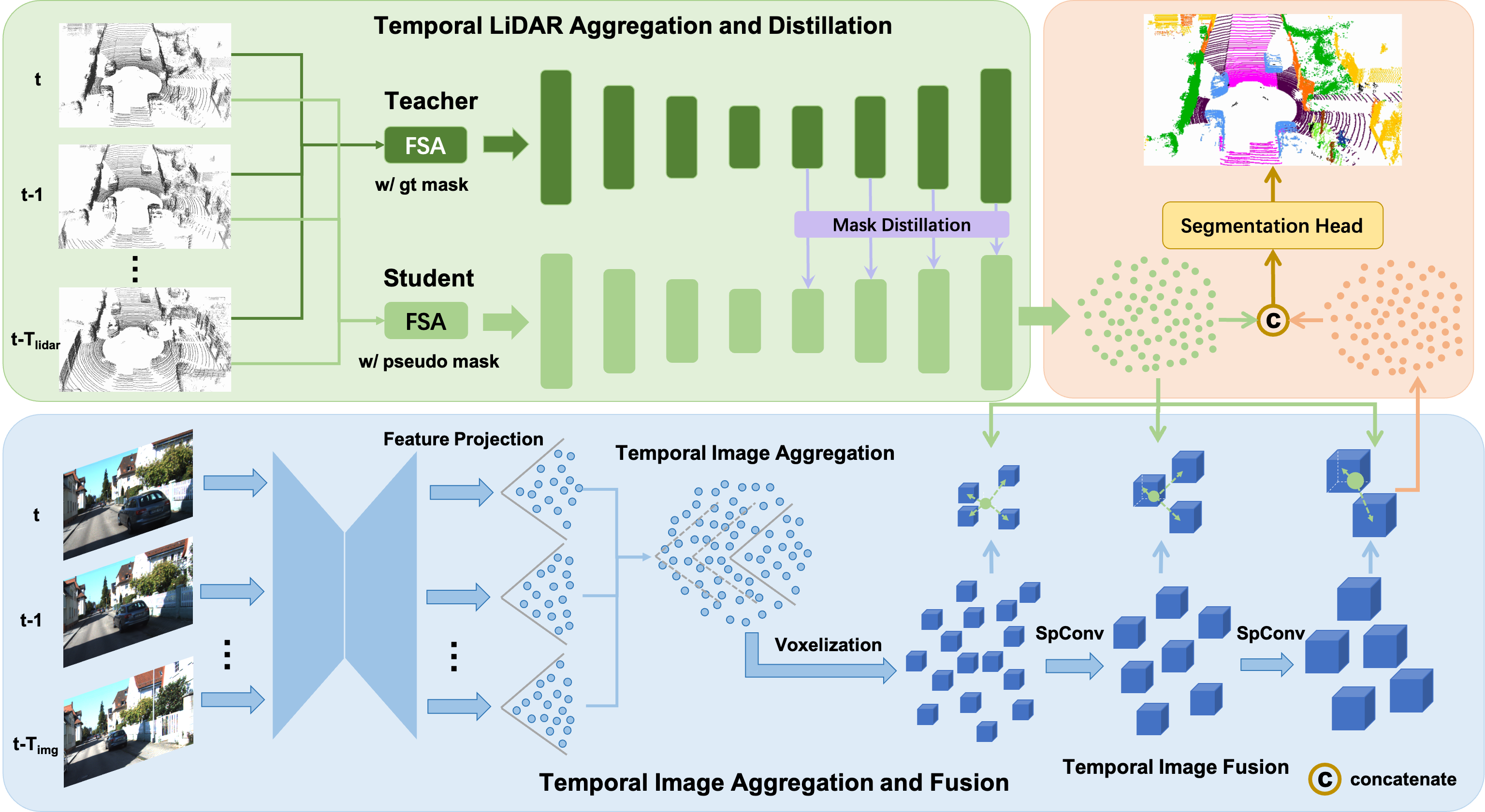
Figure 1: Overview of our Temporal Aggregation Network (TASeg). (1) Temporal LiDAR Aggregation and Distillation leverages the proposed Flexible Step Aggregation (FSA) to assign different temporal steps for different classes, and it utilizes a teacher injected with gt priors for knowledge distillation. (2) Temporal Image Aggregation and Fusion takes temporal LiDAR points as mediums to transform historical image features to the present coordinate. 3D sparse convolutions are employed to fuse temporal image features. Finally, we use temporal LiDAR points to gather voxel-wise temporal image features for temporal multi-modal fusion.

3 Methodology

3.1 Temporal LiDAR Aggregation and Distillation

A simple solution to utilize the temporal information of a consecutive point cloud sequence is to concatenate all points of the sequence, as shown in the following equation:

$$X_{t} =\text{concat}(P_{t},T_{t-1}P_{t-1},\dots,T_{t-\Delta t}P_{t-\Delta t}),$$ (1)

$$Y_{t} =\text{concat}(L_{t},L_{t-1},\dots,L_{t-\Delta t}),$$

where $P_{t-i}$ and $L_{t-i}$ denote the $(t-i)^{th}$ point cloud frame and the corresponding point-wise label. $T_{t-i}$ is the transformation matrix that transforms the coordinate from the $(t-i)^{th}$ frame to the $t^{th}$ frame. $\Delta t$ is the window size of temporal point clouds and $\text{concat}(.)$ denotes the concatenation operation. $X_{t}$ and $Y_{t}$ are the aggregated LiDAR frame and point-wise label. Although simple, there are some problems. On the one hand, direct concatenation consumes much GPU memory. On the other hand, the huge memory cost constrains the multi-frame model from utilizing more historical frames, thereby limiting the ultimate performance.

3.1.1 Flexible Step Aggregation

To reduce the GPU memory consumption, we can sample temporal frames with a step, while this method is also sub-optimal. A small step introduces huge memory overhead, whilst a large step cannot utilize sufficient temporal information. To this end, we propose Flexible Step Aggregation (FSA). Our method is based on the observation that for different classes, the model needs different amounts of temporal information. For difficult classes, such as bicycles, more points are needed to yield accurate predictions. For easy classes, such as cars and buildings, it is unnecessary to aggregate many point cloud frames for them. Based on the above analysis, we propose to assign different steps for different classes according to their learning difficulty. Specifically, we leverage historical predictions to divide the temporal point clouds into several class groups and assign a specific sampling step for each group. Then, we aggregate temporal points for each group with the corresponding step. Eventually, temporal points of all groups are concatenated with the current frame, resulting in an aggregated frame.

The group division is not strict as long as it follows the principle that more difficult classes need smaller steps. For example, we can simply divide all classes into three groups according to their segmentation performance, such as [0, 80) mIoU, [80, 90) mIoU and [90, 100] mIoU. Then, we assign the three groups with a step of 2, 4 and $\infty$ ($\infty$ means we do not aggregate temporal points for the group). To save more memory and computation without sacrificing performance, a more fine-grained division can be used. Formally, suppose we divide temporal point clouds into $g$ groups. We aggregate temporal points for the $k^{th}$ group as below:

$$X_{t}^{k} =\text{concat}(T_{o_{1}}P_{o_{1}}M_{o_{1}}^{k},\dots,T_{o_{n}}P_{o_{n}}M_{o_{n}}^{k}),$$ (2)

$$Y_{t}^{k} =\text{concat}(L_{o_{1}}M_{o_{1}}^{k},\dots,L_{o_{n}}M_{o_{n}}^{k}).$$

Here $o=\{o_{i}|o_{i}=t-i\times s_{k},i=1,2,...,n,n=\lfloor\Delta t/s_{k}\rfloor\}$. $s_{k}$ is the sampling step for the $k^{th}$ class group and $\lfloor.\rfloor$ is the floor operation. $M^{k}_{o_{i}}$ is the group mask that indicates which point of $P_{o_{i}}$ belongs to the $k^{th}$ class group. It can be obtained from historical predictions. Finally, we concatenate points and labels of all groups with the current frame:

$$X_{t} =\text{concat}(P_{t},X_{t}^{1},\dots,X_{t}^{k},\dots,X_{t}^{g}),$$ (3)

$$Y_{t} =\text{concat}(L_{t},Y_{t}^{1},\dots,X_{t}^{k},\dots,Y_{t}^{g}).$$

In this way, we discard massive redundant temporal points while maintaining essential temporal information. Since easy classes are usually large and hold a large quantity of points, the GPU memory overhead can be further reduced. Moreover, by assigning different classes with different steps, FSA actually injects historical priors into the aggregated point clouds. For classes with different steps, their patterns can be more discriminative due to their different densities (steps), which makes it easier to segment the multi-frame point clouds aggregated by FSA. Experiments in Table 4 verify that the proposed FSA can not only save memory and time costs but also achieve better performance.

3.1.2 Mask Distillation

In FSA, we use historical predictions to generate group masks, which we call pseudo masks. Since ground truth labels are more accurate than historical predictions, a natural question arises: what if we use gt masks (the group masks generated by ground truth labels) for FSA? Our experiment shows that the performance can be improved greatly. Actually, using gt masks for FSA can produce more discriminative patterns for classes with different steps. This motivates us to simulate features of a model trained on temporal point clouds aggregated with gt masks. In this way, our model is guided to learn more discriminative features to distinguish different classes. We call this Mask Distillation. Specifically, we formulate the distillation on the feature map of student $F^{s}\in\mathbb{R}^{N^{s}\times C}$ and the feature map of teacher $F^{t}\in\mathbb{R}^{N^{t}\times C}$:

$$\mathcal{L}_{\text{KD}}=\mathbb{E}[\|F^{s}m^{s}-F^{t}m^{t}\|_{2}].$$ (4)

Since temporal point clouds aggregated with pseudo masks and gt masks are different, we use masks $m^{s}$ and $m^{t}$ to select voxels that appeared in both $F^{s}$ and $F^{t}$. Note that our Mask Distillation is distinct from the methods that distill a multi-frame model to a single-frame model [32, 44]. Both the student and teacher in our method are multi-frame models.

3.2 Temporal Image Aggregation and Fusion

Previous multi-modal fusion methods only focus on leveraging present images while ignoring the precious value of temporal images. Temporal images can provide broader camera FOVs and richer information. Besides, they can enable more robust multi-modal fusion under the malfunction condition on some cameras. In this section, we provide an effective solution for aggregating temporal image features and performing temporal multi-modal fusion.

Temporal Aggregation and Fusion. Since temporal images are in different feature spaces, it is difficult to establish the relationship between different images for feature aggregation. In our method, we take temporal LiDAR points as mediums to transform temporal image features to the present coordinate with the pose information. This way, temporal image features are unified to the present 3D space. Specifically, given an image $I_{t-\Delta t}\in\mathbb{R}^{H\times W\times 3}$ and point cloud $P_{t-\Delta t}\in\mathbb{R}^{N\times 3}$, we use an image network to extract the image feature $Z_{t-\Delta t}\in\mathbb{R}^{H\times W\times C}$. According to the sensor calibration, we can establish the pixel-to-point mapping between 2D pixels and 3D points. Hence, we can project image feature $Z_{t-\Delta t}$ to 3D space, resulting in point-wise image feature $Q_{t-\Delta t}\in\mathbb{R}^{M\times C}$, where $M$ is the number of LiDAR points located on $Z_{t-\Delta t}$. By transforming $Q_{t-\Delta t}$ to the present coordinate with the pose matrix, we realize the aggregation of temporal image features:

$$\overline{X}_{t} =\text{concat}(Q_{t},T_{o_{1}}Q_{o_{1}},\dots,T_{o_{n}}Q_{o_{n}}),$$ (5)

where $o=\{o_{i}|o_{i}=t-i\times s,i=1,2,...,\lfloor\Delta t/s\rfloor\}$ and $s$ is the sampling step for temporal images. With temporal images aggregated, the FOV of the present camera is expanded greatly. Moreover, temporal image feature fusion becomes convenient because they are unified to the same 3D space. Concretely, we can use several 3D sparse convolutions to fuse aggregated temporal image features, which also endows them with geometric information, as shown in Equation 6. In addition, feature map downsampling is also utilized to generate multi-scale voxel features, providing richer information for subsequent temporal multi-modal fusion.

$$\overline{V}_{t} =\text{SparseConv}_{\text{3D}}(\text{Voxelization}(\overline{X}_{t})).$$ (6)

Temporal Multi-Modal Fusion. Benefiting from the temporal image aggregation, associating temporal image features with temporal LiDAR points also becomes convenient. Specifically, given temporal image features converted to unified voxel representation $\overline{V}_{t}$, we can establish a point-to-voxel association between temporal LiDAR points and $\overline{V}_{t}$. For each temporal LiDAR point, we generate its image feature by pooling its nearby voxel-wise temporal image features with trilinear interpolation instead of hard indexing. To extract richer image features, we perform interpolation on multi-scale feature maps. Finally, we concatenate the point cloud features and aggregated multi-scale image features, resulting in fused features, which convey powerful information of both temporal point clouds and temporal images.

2D and 3D Supervision. To make the extracted image features more informative, we add 2D supervision and 3D supervision on the 2D backbone and 3D convolutions in the image branch, respectively. The 3D supervision is just the label of point clouds. The 2D supervision is obtained by projecting labels of point clouds to the image plane.

3.3 Static-Moving Switch Augmentation

In the multi-scan task, the model is required to distinguish the motion state of movable objects. To enable the model to explore a large data space, we design an effective data augmentation, Static-Moving Switch Augmentation (SMSA). SMSA enables a movable object to switch its motion state freely, which can remarkably increase the sample quantity of static and moving objects. Concretely, considering that a unique object $b$ has the same instance id in all frames of a sequence, we can use its instance mask to crop its temporal point clouds, which is denoted as $\mathcal{B}$ = $\{\mathcal{B}_{o_{i}}|i=0,1,...,\lfloor\Delta t/s\rfloor,\mathcal{B}_{o_{i}}\in\mathbb{R}^{N\times 3}\}$. Here $o=\{o_{i}|o_{i}=t-i\times s,i=1,2,...,\lfloor\Delta t/s\rfloor\}$, $s$ is the sampling step and $\mathcal{B}_{o_{i}}$ is the temporal part of $b$ at $t_{o_{i}}$. By manipulating $\mathcal{B}$, we can change the motion state of $b$.

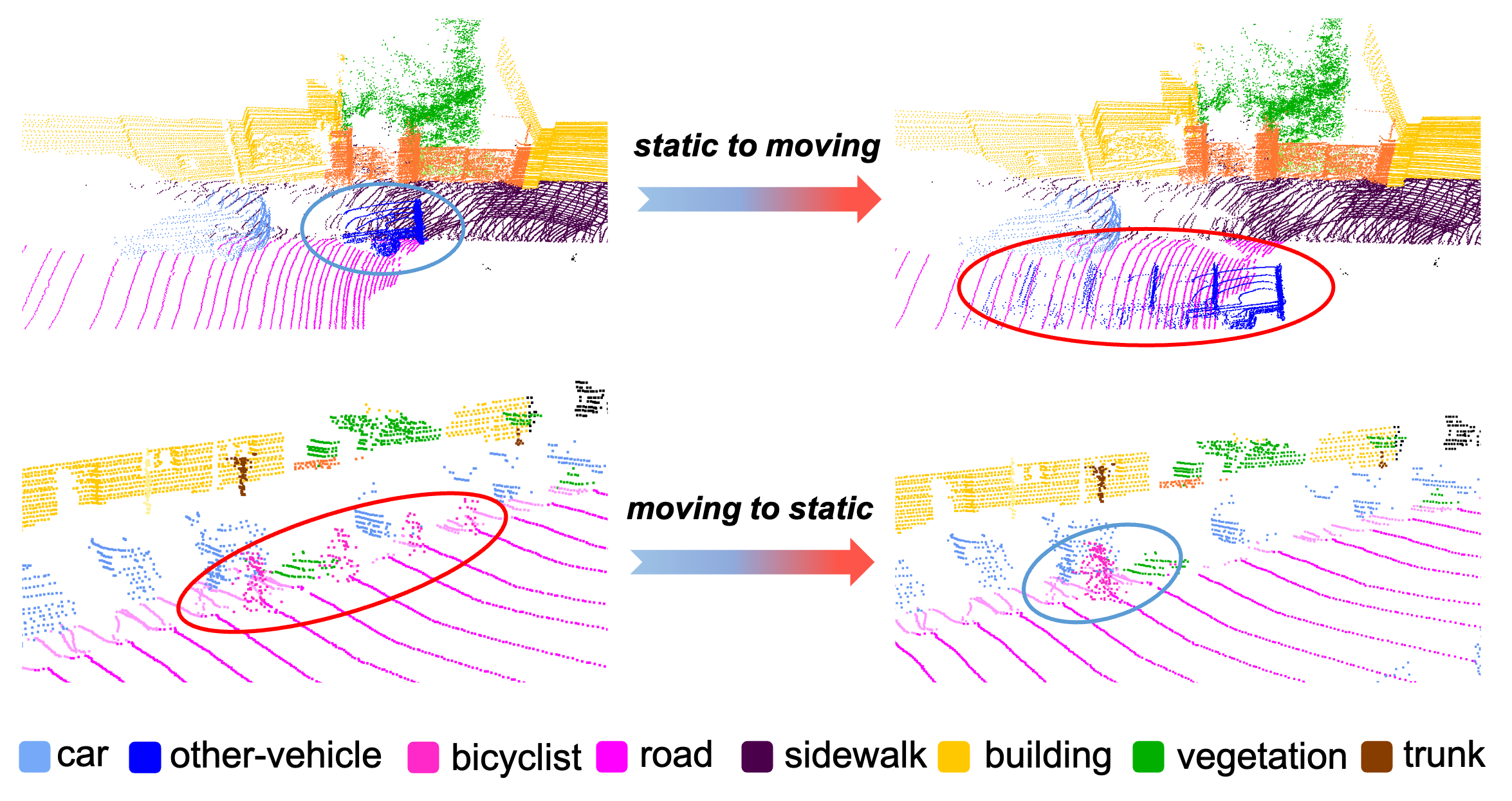
Figure 2: Visualization of the augmented samples by our Static-Moving Switch Augmentation (SMSA). Our SMSA switches the motion state by manipulating the temporal parts of objects.

Static to Moving. If $b$ is static, all temporal parts of $b$ locate at the same position, as shown in the upper-left of Figure 2. To change $b$ to a moving object, we can shift each temporal part of $b$ with an offset. Considering that objects typically move at a constant speed within a short time, we set the offset between adjacent temporal parts to be the same. For offset itself, it is a random value to increase the diversity of resulting moving samples. As for the direction of the offset, it can be roughly estimated by comparing the width and height of the minimum bounding box of $b$. Since static objects often park on the side of the road, which is crowded, the shifted temporal parts of static objects may overlap with other objects. To alleviate this, we define a set of anchor points around $b$ and a coverage area for each anchor point. Then, we shift all temporal parts of $b$ to the anchor point whose coverage area contains the fewest LiDAR points (refer to the supplementary material for more details).

Moving to Static. If $b$ is moving, different temporal parts of $b$ locate at different positions. To switch its motion state to static, we can shift all its temporal parts to the same position. In particular, we calculate the centers of each temporal part of $b$, which are denoted as $\mathcal{C}$ = $\{\mathcal{C}_{o_{i}}|\mathcal{C}_{o_{i}}\in\mathbb{R}^{3}\}$. Considering the trajectory of moving objects in a short time is approximate to a line and the speed is a constant, we simply use $q=\mathcal{C}_{o_{0}}-\mathcal{C}_{o_{1}}$ as the offset of adjacent temporal parts of $b$. Eventually, we can obtain a static object by shifting all temporal parts of $b$ to ${C}_{o_{0}}$ (see Figure 2).

It should be noted that our SMSA is an online and plug-and-play data augmentation strategy, which consumes negligible storage and computation costs.

3.4 Training Objective

The final training objective is comprised of LiDAR segmentation loss, mask distillation loss, fusion segmentation loss, 2D and 3D supervision loss on the image branch:

$$\mathcal{L}=\mathcal{L}_{\text{LiDAR}}+\alpha\mathcal{L}_{\text{KD}}+\beta\mathcal{L}_{\text{Fusion}}+\gamma(\mathcal{L}_{\text{2D}}+\mathcal{L}_{\text{3D}}),\vspace{-2mm}$$ (7)

where $\alpha,\beta,\gamma$ are the coefficients to control the effect of different losses. We set $\alpha=1,\beta=1,\gamma=1$ by default.

4 Experiments

Method	mIoU	car	bicycle	motorcycle	truck	other-veh.	person	bicyclist	motorcyclist	road	parking	sidewalk	other-gro.	building	fence	vegetation	trunk	terrain	pole	traffic sign
SqueezeSegV2 [33]	39.7	81.8	18.5	17.9	13.4	14.0	20.1	25.1	3.9	88.6	45.8	67.6	17.7	73.7	41.1	71.8	35.8	60.2	20.2	26.3
RangeNet53++ [25]	52.2	91.4	25.7	34.4	25.7	23.0	38.3	38.8	4.8	91.8	65.0	75.2	27.8	87.4	58.6	80.5	55.1	64.6	47.9	55.9
RandLA-Net [14]	55.9	94.2	29.8	32.2	43.9	39.1	48.4	47.4	9.4	90.5	61.8	74.0	24.5	89.7	60.4	83.8	63.6	68.6	51.0	50.7
SqueezeSegV3 [36]	55.9	92.5	38.7	36.5	29.6	33.0	45.6	46.2	20.1	91.7	63.4	74.8	26.4	89.0	59.4	82.0	58.7	65.4	49.6	58.9
JS3C-Net [38]	66.0	95.8	59.3	52.9	54.3	46.0	69.5	65.4	39.9	88.9	61.9	72.1	31.9	92.5	70.8	84.5	69.8	67.9	60.7	68.7
SPVNAS [31]	67.0	97.2	50.6	50.4	56.6	58.0	67.4	67.1	50.3	90.2	67.6	75.4	21.8	91.6	66.9	86.1	73.4	71.0	64.3	67.3
Cylinder3D [46]	68.9	97.1	67.6	63.8	50.8	58.5	73.7	69.2	48.0	92.2	65.0	77.0	32.3	90.7	66.5	85.6	72.5	69.8	62.4	66.2
RPVNet [37]	70.3	97.6	68.4	68.7	44.2	61.1	75.9	74.4	43.4	93.4	70.3	80.7	33.3	93.5	72.1	86.5	75.1	71.7	64.8	61.4
(AF)2-S3Net [5]	70.8	94.3	63.0	81.4	40.2	40.0	76.4	81.7	77.7	92.0	66.8	76.2	45.8	92.5	69.6	78.6	68.0	63.1	64.0	73.3
PVKD [13]	71.2	97.0	69.3	53.5	67.9	60.2	75.1	73.5	50.5	91.8	77.5	70.9	41.0	92.4	69.4	86.5	73.8	71.9	64.9	65.8
2DPASS [39]	72.9	97.0	63.6	63.4	61.1	61.5	77.9	81.3	74.1	89.7	67.4	74.7	40.0	93.5	72.9	86.2	73.9	71.0	65.0	70.4
SphereFormer [19]	74.8	97.5	70.1	70.5	59.6	67.7	79.0	80.4	75.3	91.8	69.7	78.2	41.3	93.8	72.8	86.7	75.1	72.4	66.8	72.9
UniSeg [24]	75.2	97.9	71.9	75.2	63.6	74.1	78.9	74.8	60.6	92.6	74.0	79.5	46.1	93.4	72.7	87.5	76.3	73.1	68.3	68.5
TASeg (Ours)	76.5	97.7	71.8	71.4	65.2	78.7	79.9	84.6	78.6	91.6	74.0	78.0	39.3	93.5	73.4	86.6	75.0	71.7	69.6	73.8

Table 1: Comparison with state-of-the-arts on SemanticKITTI test set (single-scan). All results can be found on the online leaderboard.

Method	mIoU	car-s	car-m	truc.-s	truc.-m	othe.-s	othe.-m	pers.-s	pers.-m	bicy.-s	bicy.-m	moto.-s	moto.-m
LatticeNet [29]	45.2	91.1	54.8	29.7	3.5	23.1	0.6	6.8	49.9	0.0	44.6	0.0	64.3
TemporalLidarSeg [9]	47.0	92.1	68.2	39.2	2.1	35.0	12.4	14.4	40.4	0.0	42.8	0.0	12.9
(AF)2-S3Net [5]	56.9	91.8	65.3	15.7	5.6	27.5	3.9	16.4	67.6	15.1	66.4	67.1	59.6
MarS3D [22]	52.7	95.1	78.4	39.7	5.1	36.6	10.0	16.2	58.0	1.2	67.3	0.0	36.3
SVQNet [4]	60.5	96.0	80.1	41.0	5.1	60.4	7.1	28.7	85.1	0.0	72.4	0.0	88.1
2DPASS [39]	62.4	96.2	82.1	48.2	16.1	52.7	3.8	35.4	80.3	7.9	71.2	62.0	73.1
TASeg (Ours)	65.7	94.8	72.8	53.6	35.2	71.4	53.2	36.7	80.4	32.4	75.2	12.3	89.6

Table 2: Comparison to the state-of-the-art methods on SemanticKITTI test set (multi-scan). -s indicates static and -m stands for moving.

Datasets & Evaluation Metrics. Following [46, 13], we evaluate the performance on two popular LiDAR segmentation benchmarks, i.e., SemanticKITTI and nuScenes. SemanticKITTI contains 22 point cloud sequences, where sequences 0-10, 8, 11-21 are selected as training, validation and testing, respectively. As for nuScenes, it collects 1, 000 driving scenes, where 850 scenes are chosen for training and validation, and the remaining 150 scenes are used for testing. We conduct experiments on three tracks, i.e., SemanticKITTI single-scan and multi-scan semantic segmentation and nuScenes semantic segmentation.

Implementation Details. We use the MinkowskiNet [7] re-implemented by PCSeg [23] as our baseline. Our TASeg is trained with the SGD [28] optimizer on 4 A100 GPUs with batch size 6 for 12 and 36 epochs on SemanticKITTI and nuScenes datasets. The learning rate and weight decay are set to 0.02 and 0.0001. The window size of temporal point clouds is set to 16. Due to a large redundancy of images, we use a step of 12 and a window size of 48 for temporal images. Our data augmentation strategy includes random flipping, rotation, scaling, transformation, LaserMix [16] and PolarMix [35]. During the inference, the LiDAR semantic predictions and image features of the previous timestamp can be saved, so there is no time cost for generating historical predictions and processing temporal image aggregation. More details are provided in the supplementary material.

4.1 Comparison with State-of-the-art Methods

We compare our TASeg with state-of-the-art LiDAR segmentation methods on SemanticKITTI single-scan and multi-scan track, and nuScenes LiDAR semantic segmentation track, as summarized in Table 1, 2 and 3. On the SemanticKITTI single-scan track, our TASeg is 1.3 mIoU higher than UniSeg [24], the best-performing published algorithm on the SemanticKITTI single-scan leaderboard. On the SemanticKITTI multi-scan track, our approach outperforms the best multi-scan method 2DPASS [39] by 3.3 mIoU. For nuScenes LiDAR semantic segmentation, we also achieve superior performance over previous algorithms. As shown in Table 3, the proposed approach surpasses the UniSeg [24] by 1.1 mIoU. In particular, our approach holds the highest entry on all three tracks. These encouraging results strongly show the effectiveness of our approach.

Method	mIoU	barrier	bicycle	bus	car	construction	motorcycle	pedestrian	traffic-cone	trailer	truck	driveable	other-flat	sidewalk	terrain	manmade	vegetation
Cylinder3D [46]	77.2	82.8	29.8	84.3	89.4	63.0	79.3	77.2	73.4	84.6	69.1	97.7	70.2	80.3	75.5	90.4	87.6
SPVCNN [31]	77.4	80.0	30.0	91.9	90.8	64.7	79.0	75.6	70.9	81.0	74.6	97.4	69.2	80.0	76.1	89.3	87.1
2D3DNet [11]	80.0	83.0	59.4	88.0	85.1	63.7	84.4	82.0	76.0	84.8	71.9	96.9	67.4	79.8	76.0	92.1	89.2
2DPASS [39]	80.8	81.7	55.3	92.0	91.8	73.3	86.5	78.5	72.5	84.7	75.5	97.6	69.1	79.9	75.5	90.2	88.0
LidarMultiNet [41]	81.4	80.4	48.4	94.3	90.0	71.5	87.2	85.2	80.4	86.9	74.8	97.8	67.3	80.7	76.5	92.1	89.6
MSeg3D [20]	81.1	83.1	42.5	94.9	92.0	67.1	78.6	85.7	80.5	87.5	77.3	97.7	69.8	81.2	77.8	92.4	90.1
SphereFormer [19]	81.9	83.3	39.2	94.7	92.5	77.5	84.2	84.4	79.1	88.4	78.3	97.9	69.0	81.5	77.2	93.4	90.2
UniSeg [24]	83.5	85.9	71.2	92.1	91.6	80.5	88.0	80.9	76.0	86.3	76.7	97.7	71.8	80.7	76.7	91.3	88.8
TASeg (Ours)	84.6	87.1	69.4	90.5	92.2	78.7	90.4	86.3	81.9	88.3	75.9	97.8	70.9	81.0	78.2	93.4	91.2

Table 3: Performance comparison with start-of-the-art methods on nuScenes test set.

4.2 Ablation studies

We examine the effect of each component through detailed ablations. Unless otherwise specified, the following experiments are trained on the training set of the SemanticKITTI single-scan task and evaluated on the validation set.

Effect of Flexible Step Aggregation.

In Table 4, we compare our FSA with other multi-frame algorithms. MSeg3D [20] utilizes temporal point clouds by directly concatenating all points, which introduces a large memory consumption and achieves limited improvement. SVQNet [4] leverages cross-attention to fuse temporal features while it can only handle fewer LiDAR scans. When increasing LiDAR scans, the memory overhead is also huge. Our FSA assigns different classes with different temporal steps, which can leverage long-term temporal information with less memory and time costs. Moreover, thanks to the utilization of historical priors, our FSA achieves better results (71.3 mIoU) than directly concatenating (69.9 mIoU), given the same temporal window size. To explore the effect of different window sizes on FSA, we present Table 5. Results show that the performance is saturated with a window size of 24.

Effect of Group Division.

To investigate the effect of different group divisions for FSA, we provide Table 6. For division1, we simply divide all classes into three groups according to their performance on the val set. The group1 consists of the classes in [90, 100) mIoU, such as cars and roads. The group2 consists of classes in [80, 90) mIoU, such as motorcycles. The group3 contains the remaining classes. We assign group1, group2 and group3 with the step of $\infty$, 4 and 2. A step of $\infty$ means we do not aggregate temporal points for classes in the group due to their near-saturate performances. The result shows that division1 can reduce the time and memory costs largely compared to directly stacking (the $2^{st}$ row in Table 4). We can also use performance top1-6, top6-12, and top12-19 for division, resulting in division2. The group division is robust as long as it follows the principle that more difficult classes need smaller steps. To further reduce the memory consumption, we can finetune the group division, such as moving large-size classes (e.g. other-ground and terrain) in group3 to group2 (division3) or moving large-size classes in group3 and group2 to a new group with step of 8 (division4). Besides, we can divide each class group into a close and a distant group according to the distance (such as 30 m). Considering close areas need fewer temporal points, we can use twice the original step for temporal aggregation of close groups (division5).

Method	Latency	Memory	mIoU
Baseline	63ms	5.0G	68.9
+ MSeg3D†	284ms	69.7G	69.9
+ SVQNet†	121ms	15.4G	69.5
+ FSA	79ms	8.5G	71.3
+ FSA w/ gt mask	79ms	8.5G	75.9
+ FSA + M.D.	79ms	8.5G	71.8
+ FSA + M.D. $\times 0.75$	72ms	6.9G	71.6

Table 4: Comparison with different multi-frame algorithms. † represents our re-implementation. “M.D.” represents Mask Distillation. “$\times 75$” represents that we reduce the model parameters to 75%.

Window size	4	8	12	16	20	24	28
mIoU	69.9	70.4	70.9	71.3	71.4	71.6	71.4

Table 5: Ablation on different window sizes for FSA.

Method	Latency	Memory	mIoU
FSA w/ division1	92ms	14.1G	70.8
FSA w/ division2	83ms	7.2G	70.6
FSA w/ division3	79ms	8.5G	71.3
FSA w/ division4	74ms	7.7G	71.2
FSA w/ division5	74ms	7.4G	71.2

Table 6: Ablation on different group divisions for FSA.

Effect of Mask Distillation.

At the $5^{th}$ row of Table 4, we use gt masks of historical frames for FSA. The performance is greatly boosted. Considering we cannot get ground truth at inference, we use it as a teacher to distill the model trained with pseudo masks. The result shows that the student is improved by 0.5 mIoU after distillation. With 75% model complexity, we can further reduce the time and memory cost and still achieve a leading performance.

Effect of Temporal Image Aggregation and Fusion.

TIAF delivers a temporal multi-modal fusion scheme to make full use of temporal images. As shown in Table 7, with zero image, only TLAD is used, achieving 71.8 mIoU. With one image, only present images are utilized. Due to the limited FOV of the present camera, only part of the LiDAR points can gather image features, which limits the multi-modal fusion. Our TIAF leverages temporal images to enlarge the FOV of the camera and enhance present features. The results show that with the number of images increasing, the performance rises gradually, which verifies the effectiveness of our TIAF. When using seven temporal images, we achieve 1.0 mIoU improvement on the strong baseline. Note that there is no extra cost to generate historical image features because we can save them at the past moments.

Num of images	0	1	3	5	7
mIoU	71.8	72.1	72.4	72.7	72.8

Table 7: Ablation on the number of temporal images for TIAF.

Exp	2D Sup.	3D Sup.	Multi-Scale	mIoU
(a)		✓	✓	72.4
(b)	✓		✓	72.5
(c)	✓	✓		72.4
(d)	✓	✓	✓	72.7

Table 8: Effect of different supervisions and multi-scale for TIAF.

We also provide the ablation on different supervisions and multi-scale features for TIAF in Table 8. In TIAF, we leverage 2D and 3D supervision to guide the extracted image features to be more conducive for segmentation. Multi-scale is also used to provide more discriminative features. The result shows that each of the designs is beneficial for final performance. Note that our temporal multi-modal method is orthogonal to other single-frame multi-modal methods. We use a simple pixel-to-point mapping at the feature projection stage. More complex methods [20, 24] can also be utilized, but it is not the focus of our TIAF.

Effect of Static-Moving Switch Augmentation.

To verify our SMSA, we present Table 9. From the results, we can find that without SMSA, the accuracy of the model on many classes is lower than 10 IoU. After using SMSA, the performance of moving truck, moving other-vehicle and static bicyclist classes is improved by more than 20 IoU, and the overall performance boosts from 61.3 mIoU to 65.7 mIoU, which strongly demonstrates the efficacy of our SMSA.

SMSA	mIoU	car-s	car-m	truc.-s	truc.-m	othe.-s	othe.-m	pers.-s	pers.-m	bicy.-s	bicy.-m	moto.-s	moto.-m
	61.3	95.6	79.3	49.2	9.1	61.0	5.7	39.0	87.0	0.0	72.6	4.3	76.4
✓	65.7	94.8	72.8	53.6	35.2	71.4	53.2	36.7	80.4	32.4	75.2	12.3	89.6

Table 9: Ablation study of our SMSA on the SemanticKITTI test benchmark of the multi-scan track.

Generalization to More Architectures.

In addition to MinkowskiNet, we also validate our temporal aggregation method on Cylinder3D [46] and SPVNAS [31]. Detailed results are summarized in Table 10. Our TASeg brings impressive improvements to both baselines, which demonstrates the strong generalization ability of our method.

Method	mIoU
Cylinder3D [46]†	66.0
Cylinder3D [46]†+ TASeg	69.6
SPVNAS [31]†	68.6
SPVNAS [31]†+ TASeg	72.7

Table 10: Performance of applying our TASeg to different baselines. † represents our re-implementation.

Comparison on Complexity, Latency and Accuracy.

As shown in Table 11, when not utilizing temporal images, our TASeg achieves superior performance than other methods with comparable or less complexity and latency. With temporal images, TASeg can maintain lower complexity and latency than UniSeg [24] while achieving higher accuracy. Besides, with 75% parameters, the latency of TASeg can be further reduced, and the accuracy is not affected much.

Method	Input	Params	Latency	mIoU
MinkowskiNet†	L	37.9M	63ms	68.4
Cylinder3D†	L	55.9M	75ms	66.0
SPVNAS†	L	96.7M	105ms	68.6
RPVNet†	L	119.0M	110ms	68.9
UniSeg	L+C	147.6M	145ms	71.3
TASeg wo/ TIAF	L+T	37.9M	79ms	71.8
TASeg	L+C+T	46.7M	116ms	72.7
TASeg $\times 0.75$	L+C+T	27.4M	108ms	72.5

Table 11: Comparison of the model complexity, latency and accuracy on SemanticKITTI val set. † represents our re-implementation on NVIDIA A100 for a fair comparison. “L”,“C” and “T” represent LiDAR, Camera and Temporal data, respectively.

5 Conclusion

In this paper, we present TASeg to fully exploit temporal point clouds and temporal images. Our TASeg is comprised of TLAD, TIAF and SMSA. We perform extensive experiments to validate the efficacy of each component. Moreover, our TASeg set a new state-of-the-art on three challenging tracks, demonstrating the superiority of our method.

6 Acknowledgements

This work was supported in part by The National Nature Science Foundation of China (Grant Nos: 62273301, 62273302, 62036009, 61936006, 62273303), in part by Yongjiang Talent Introduction Programme (Grant No: 2022A-240-G, 2023A-197-G), in part by the National Key R&D Program of China (NO.2022ZD0160100). This work was done during the first author’s internship at Shanghai AI Laboratory.

References

- Aygun et al. [2021] Mehmet Aygun, Aljosa Osep, Mark Weber, Maxim Maximov, Cyrill Stachniss, Jens Behley, and Laura Leal-Taixé. 4d panoptic lidar segmentation. In Proceedings of the IEEE/CVF Conference on Computer Vision and Pattern Recognition, pages 5527–5537, 2021.
- Cao et al. [2020] Hanwen Cao, Yongyi Lu, Cewu Lu, Bo Pang, Gongshen Liu, and Alan Yuille. Asap-net: Attention and structure aware point cloud sequence segmentation. arXiv preprint arXiv:2008.05149, 2020.
- Chen et al. [2023a] Li Chen, Penghao Wu, Kashyap Chitta, Bernhard Jaeger, Andreas Geiger, and Hongyang Li. End-to-end autonomous driving: Challenges and frontiers. arXiv preprint arXiv:2306.16927, 2023a.
- Chen et al. [2023b] Xuechao Chen, Shuangjie Xu, Xiaoyi Zou, Tongyi Cao, Dit-Yan Yeung, and Lu Fang. Svqnet: Sparse voxel-adjacent query network for 4d spatio-temporal lidar semantic segmentation. In Proceedings of the IEEE/CVF International Conference on Computer Vision, pages 8569–8578, 2023b.
- Cheng et al. [2021] Ran Cheng, Ryan Razani, Ehsan Taghavi, Enxu Li, and Bingbing Liu. (af)2-S3Net: Attentive Feature Fusion with Adaptive Feature Selection for Sparse Semantic Segmentation Network. In IEEE Conference on Computer Vision and Pattern Recognition, pages 12547–12556, 2021.
- Choy et al. [2019a] Christopher Choy, JunYoung Gwak, and Silvio Savarese. 4d spatio-temporal convnets: Minkowski convolutional neural networks. In CVPR, 2019a.
- Choy et al. [2019b] Christopher Choy, JunYoung Gwak, and Silvio Savarese. 4D Spatio-Temporal ConvNets: Minkowski Convolutional Neural Networks. In IEEE/CVF Conference on Computer Vision and Pattern Recognition, pages 3075–3084, 2019b.
- Dewan and Burgard [2020] Ayush Dewan and Wolfram Burgard. Deeptemporalseg: Temporally consistent semantic segmentation of 3d lidar scans. In 2020 IEEE International Conference on Robotics and Automation (ICRA), pages 2624–2630. IEEE, 2020.
- Duerr et al. [2020] Fabian Duerr, Mario Pfaller, Hendrik Weigel, and Jürgen Beyerer. Lidar-based recurrent 3d semantic segmentation with temporal memory alignment. In 2020 International Conference on 3D Vision (3DV), pages 781–790. IEEE, 2020.
- El Madawi et al. [2019] Khaled El Madawi, Hazem Rashed, Ahmad El Sallab, Omar Nasr, Hanan Kamel, and Senthil Yogamani. Rgb and lidar fusion based 3d semantic segmentation for autonomous driving. In IEEE Intelligent Transportation Systems Conference, pages 7–12, 2019.
- Genova et al. [2021] Kyle Genova, Xiaoqi Yin, Abhijit Kundu, Caroline Pantofaru, Forrester Cole, Avneesh Sud, Brian Brewington, Brian Shucker, and Thomas Funkhouser. Learning 3d semantic segmentation with only 2d image supervision. In 3DV, 2021.
- Hinton et al. [2015] Geoffrey Hinton, Oriol Vinyals, and Jeff Dean. Distilling the knowledge in a neural network. arXiv preprint arXiv:1503.02531, 2015.
- Hou et al. [2022] Yuenan Hou, Xinge Zhu, Yuexin Ma, Chen Change Loy, and Yikang Li. Point-to-Voxel Knowledge Distillation for LiDAR Semantic Segmentation. In IEEE Conference on Computer Vision and Pattern Recognition, pages 8479–8488, 2022.
- Hu et al. [2020] Qingyong Hu, Bo Yang, Linhai Xie, Stefano Rosa, Yulan Guo, Zhihua Wang, Niki Trigoni, and Andrew Markham. Randla-net: Efficient semantic segmentation of large-scale point clouds. Proceedings of the IEEE Conference on Computer Vision and Pattern Recognition, 2020.
- Kong et al. [2023a] Lingdong Kong, Youquan Liu, Runnan Chen, Yuexin Ma, Xinge Zhu, Yikang Li, Yuenan Hou, Yu Qiao, and Ziwei Liu. Rethinking range view representation for lidar segmentation. In Proceedings of the IEEE/CVF International Conference on Computer Vision, pages 228–240, 2023a.
- Kong et al. [2023b] Lingdong Kong, Jiawei Ren, Liang Pan, and Ziwei Liu. Lasermix for semi-supervised lidar semantic segmentation. In Proceedings of the IEEE/CVF Conference on Computer Vision and Pattern Recognition, pages 21705–21715, 2023b.
- Kreuzberg et al. [2022] Lars Kreuzberg, Idil Esen Zulfikar, Sabarinath Mahadevan, Francis Engelmann, and Bastian Leibe. 4d-stop: Panoptic segmentation of 4d lidar using spatio-temporal object proposal generation and aggregation. In European Conference on Computer Vision, pages 537–553. Springer, 2022.
- Krispel et al. [2020] Georg Krispel, Michael Opitz, Georg Waltner, Horst Possegger, and Horst Bischof. Fuseseg: Lidar point cloud segmentation fusing multi-modal data. In IEEE/CVF Winter Conference on Applications of Computer Vision, pages 1874–1883, 2020.
- Lai et al. [2023] Xin Lai, Yukang Chen, Fanbin Lu, Jianhui Liu, and Jiaya Jia. Spherical transformer for lidar-based 3d recognition. arXiv preprint arXiv:2303.12766, 2023.
- Li et al. [2023a] Jiale Li, Hang Dai, Hao Han, and Yong Ding. MSeg3D: Multi-modal 3D Semantic Segmentation for Autonomous Driving. arXiv preprint arXiv:2303.08600, 2023a.
- Li et al. [2023b] Zhenyu Li, Zehui Chen, Xianming Liu, and Junjun Jiang. Depthformer: Exploiting long-range correlation and local information for accurate monocular depth estimation. Machine Intelligence Research, 20(6):837–854, 2023b.
- Liu et al. [2023a] Jiahui Liu, Chirui Chang, Jianhui Liu, Xiaoyang Wu, Lan Ma, and Xiaojuan Qi. Mars3d: A plug-and-play motion-aware model for semantic segmentation on multi-scan 3d point clouds. In Proceedings of the IEEE/CVF Conference on Computer Vision and Pattern Recognition, pages 9372–9381, 2023a.
- Liu et al. [2023b] Youquan Liu, Yeqi Bai, Lingdong Kong, Runnan Chen, Yuenan Hou, Botian Shi, and Yikang Li. Pcseg: An open source point cloud segmentation codebase. https://github.com/PJLab-ADG/PCSeg, 2023b.
- Liu et al. [2023c] Youquan Liu, Runnan Chen, Xin Li, Lingdong Kong, Yuchen Yang, Zhaoyang Xia, Yeqi Bai, Xinge Zhu, Yuexin Ma, Yikang Li, et al. Uniseg: A unified multi-modal lidar segmentation network and the openpcseg codebase. In Proceedings of the IEEE/CVF International Conference on Computer Vision, pages 21662–21673, 2023c.
- Milioto et al. [2019] Andres Milioto, Ignacio Vizzo, Jens Behley, and Cyrill Stachniss. Rangenet++: Fast and accurate lidar semantic segmentation. In Proc. of the IEEE/RSJ Intl. Conf. on Intelligent Robots and Systems (IROS), 2019.
- Qi et al. [2017a] Charles R Qi, Hao Su, Kaichun Mo, and Leonidas J Guibas. Pointnet: Deep learning on point sets for 3d classification and segmentation. In Proceedings of the IEEE conference on computer vision and pattern recognition, pages 652–660, 2017a.
- Qi et al. [2017b] Charles Ruizhongtai Qi, Li Yi, Hao Su, and Leonidas J Guibas. Pointnet++: Deep hierarchical feature learning on point sets in a metric space. In Advances in neural information processing systems, pages 5099–5108, 2017b.
- Robbins and Monro [1951] Herbert Robbins and Sutton Monro. A Stochastic Approximation Method. The annals of mathematical statistics, pages 400–407, 1951.
- Rosu et al. [2019] Radu Alexandru Rosu, Peer Schütt, Jan Quenzel, and Sven Behnke. Latticenet: Fast point cloud segmentation using permutohedral lattices. arXiv preprint arXiv:1912.05905, 2019.
- Shi et al. [2020] Hanyu Shi, Guosheng Lin, Hao Wang, Tzu-Yi Hung, and Zhenhua Wang. Spsequencenet: Semantic segmentation network on 4d point clouds. In CVPR, 2020.
- Tang et al. [2020] Haotian Tang, Zhijian Liu, Shengyu Zhao, Yujun Lin, Ji Lin, Hanrui Wang, and Song Han. Searching Efficient 3D Architectures with Sparse Point-Voxel Convolution. In European Conference on Computer Vision, pages 685–702. Springer, 2020.
- Tang et al. [2019] Jiexiong Tang, John Folkesson, and Patric Jensfelt. Sparse2dense: From direct sparse odometry to dense 3-d reconstruction. IEEE Robotics and Automation Letters, 4(2):530–537, 2019.
- Wu et al. [2019] Bichen Wu, Xuanyu Zhou, Sicheng Zhao, Xiangyu Yue, and Kurt Keutzer. Squeezesegv2: Improved model structure and unsupervised domain adaptation for road-object segmentation from a lidar point cloud. In 2019 International Conference on Robotics and Automation (ICRA), pages 4376–4382. IEEE, 2019.
- Wu et al. [2022] Dong Wu, Man-Wen Liao, Wei-Tian Zhang, Xing-Gang Wang, Xiang Bai, Wen-Qing Cheng, and Wen-Yu Liu. Yolop: You only look once for panoptic driving perception. Machine Intelligence Research, 19(6):550–562, 2022.
- Xiao et al. [2022] Aoran Xiao, Jiaxing Huang, Dayan Guan, Kaiwen Cui, Shijian Lu, and Ling Shao. PolarMix: A General Data Augmentation Technique for LiDAR Point Clouds. arXiv preprint arXiv:2208.00223, 2022.
- Xu et al. [2020] Chenfeng Xu, Bichen Wu, Zining Wang, Wei Zhan, Peter Vajda, Kurt Keutzer, and Masayoshi Tomizuka. Squeezesegv3: Spatially-adaptive convolution for efficient point-cloud segmentation. In European Conference on Computer Vision, pages 1–19. Springer, 2020.
- Xu et al. [2021] Jianyun Xu, Ruixiang Zhang, Jian Dou, Yushi Zhu, Jie Sun, and Shiliang Pu. RPVnet: A Deep and Efficient Range-Point-Voxel Fusion Network for Lidar Point Cloud Segmentation. In IEEE International Conference on Computer Vision, pages 16024–16033, 2021.
- Yan et al. [2021] Xu Yan, Jiantao Gao, Jie Li, Ruimao Zhang, Zhen Li, Rui Huang, and Shuguang Cui. Sparse single sweep lidar point cloud segmentation via learning contextual shape priors from scene completion. In Proceedings of the AAAI Conference on Artificial Intelligence, pages 3101–3109, 2021.
- Yan et al. [2022] Xu Yan, Jiantao Gao, Chaoda Zheng, Chao Zheng, Ruimao Zhang, Shuguang Cui, and Zhen Li. 2DPASS: 2D Priors Assisted Semantic Segmentation on LiDAR Point Clouds. In European Conference on Computer Vision, 2022.
- Yang et al. [2022] Jihan Yang, Shaoshuai Shi, Runyu Ding, Zhe Wang, and Xiaojuan Qi. Towards efficient 3d object detection with knowledge distillation. Advances in Neural Information Processing Systems, 35:21300–21313, 2022.
- Ye et al. [2022] Dongqiangzi Ye, Zixiang Zhou, Weijia Chen, Yufei Xie, Yu Wang, Panqu Wang, and Hassan Foroosh. Lidarmultinet: Towards a unified multi-task network for lidar perception. arXiv preprint arXiv:2209.09385, 2022.
- Yurtsever et al. [2020] Ekim Yurtsever, Jacob Lambert, Alexander Carballo, and Kazuya Takeda. A survey of autonomous driving: Common practices and emerging technologies. IEEE access, 8:58443–58469, 2020.
- Zhang et al. [2023] Zhiwei Zhang, Zhizhong Zhang, Qian Yu, Ran Yi, Yuan Xie, and Lizhuang Ma. Lidar-camera panoptic segmentation via geometry-consistent and semantic-aware alignment. In Proceedings of the IEEE/CVF International Conference on Computer Vision, pages 3662–3671, 2023.
- Zheng et al. [2022] Wu Zheng, Li Jiang, Fanbin Lu, Yangyang Ye, and Chi-Wing Fu. Boosting single-frame 3d object detection by simulating multi-frame point clouds. In Proceedings of the 30th ACM International Conference on Multimedia, pages 4848–4856, 2022.
- Zhu et al. [2023] Minghan Zhu, Shizhong Han, Hong Cai, Shubhankar Borse, Maani Ghaffari, and Fatih Porikli. 4d panoptic segmentation as invariant and equivariant field prediction. In Proceedings of the IEEE/CVF International Conference on Computer Vision (ICCV), pages 22488–22498, 2023.
- Zhu et al. [2021] Xinge Zhu, Hui Zhou, Tai Wang, Fangzhou Hong, Yuexin Ma, Wei Li, Hongsheng Li, and Dahua Lin. Cylindrical and Asymmetrical 3D Convolution Networks for Lidar Segmentation. In IEEE Conference on Computer Vision and Pattern Recognition, pages 9939–9948, 2021.
- Zhuang et al. [2021] Zhuangwei Zhuang, Rong Li, Kui Jia, Qicheng Wang, Yuanqing Li, and Mingkui Tan. Perception-aware multi-sensor fusion for 3d lidar semantic segmentation. In ICCV, 2021.