On Lower Bounding Minimal Model Count

Abstract

Minimal models of a Boolean formula play a pivotal role in various reasoning tasks. While previous research has primarily focused on qualitative analysis over minimal models; our study concentrates on the quantitative aspect, specifically counting of minimal models. Exact counting of minimal models is strictly harder than $\#\mathsf{P}$, prompting our investigation into establishing a lower bound for their quantity, which is often useful in related applications. In this paper, we introduce two novel techniques for counting minimal models, leveraging the expressive power of answer set programming: the first technique employs methods from knowledge compilation, while the second one draws on recent advancements in hashing-based approximate model counting. Through empirical evaluations, we demonstrate that our methods significantly improve the lower bound estimates of the number of minimal models, surpassing the performance of existing minimal model reasoning systems in terms of runtime.

1 Introduction

Given a propositional formula $F$, a model $\sigma\models F$ is minimal if $\forall\sigma\textprime\subset\sigma$, it holds that $\sigma\textprime\not\models F$ (Angiulli et al., 2014). Minimal model reasoning is fundamental to several tasks in artificial intelligence, including circumscription (McCarthy, 1980; Lifschitz, 1985), default logic (Reiter, 1980), diagnosis (De Kleer et al., 1992), and deductive databases under the generalized closed-world assumption (Minker, 1982). Although not new, minimal model reasoning has been the subject of several studies (Eiter and Gottlob, 1993; Ben-Eliyahu and Dechter, 1996; Ben-Eliyahu, 2005; Kirousis and Kolaitis, 2003), covering tasks such as minimal model finding (finding a single minimal model), minimal model checking (deciding whether a model is minimal), and minimal model entailment and membership (deciding whether a literal belongs to all minimal models or some minimal models, respectively) (Ben-Eliyahu and Palopoli, 1997).

Complexity analysis has established that minimal model reasoning is intractable, tractable only for specific subclasses of CNF (Conjunctive Normal Form) formulas. Typically, finding one minimal model for positive CNF formulas is in $\mathsf{P}^{\mathsf{NP}[\mathcal{O}(\log{n})]}$-hard (Cadoli, 1992b ). Additionally, checking whether a model is minimal is $\mathsf{co}$-$\mathsf{NP}$-complete (Cadoli, 1992a ), whereas queries related to entailment and membership are positioned at the second level of the polynomial hierarchy (Eiter and Gottlob, 1993).

This study delves into a nuanced reasoning task on minimal models, extending beyond the simplistic binary version of decision-based queries. Our focus shifts towards quantitative reasoning with respect to minimal models. Specifically, we aim to count the number of minimal models for a given propositional formula. While enumerating a single minimal model is insufficient in many applications, counting the number of minimal models provides a useful metric for related measures (Thimm, 2016; Hunter et al., 2008). Apart from specific structures of Boolean formulas, exact minimal model counting is $\#\mathsf{co}$-$\mathsf{NP}$-complete (Kirousis and Kolaitis, 2003), established through subtractive reductions.

Although minimal models can theoretically be counted by iteratively employing minimal model finding oracles, this approach is practical only for a relatively small number of minimal models and becomes impractical as their number increases. Advanced model counting techniques have scaled to a vast number of models through sophisticated knowledge compilation methods (Darwiche, 2004; Thurley, 2006), which involve transforming an input formula into a specific representation that enables efficient model counting based on the size of this new representation. However, applying knowledge compilation to minimal model counting presents unique challenges, which is elaborated in Section 4. Beyond knowledge compilation, approximate model counting has emerged as a successful strategy for estimating the number of models with probabilistic guarantees (Chakraborty et al., 2013). In particular, the hashing-based technique, which partitions the search space into smaller, roughly equal partitions using randomly generated XOR constraints (Gomes et al., 2021),  has attracted significant attention. The model count can be estimated by enumerating the models within one randomly chosen partition (Chakraborty et al., 2013).

Our empirical study reveals that both approaches to minimal model counting face scalability issues in practical scenarios. Furthermore, knowing a lower bound of the model count is still useful in many applications and is often computed in the model counting literature (Gomes et al., 2007). Some applications require the enumeration of all minimal models (Jannach et al., 2016; Bozzano et al., 2022), but complete enumeration becomes infeasible for a large number of minimal models. Here, the lower bound of the number of minimal models provides a useful criterion for assessing the feasibility of enumerating all minimal models. Knowing this lower bound of the model count is often beneficial to estimate the size of the search space, which enables more specific targeting within the search space (Fichte et al., 2022). Consequently, our research shifts focus from counting all minimal models to determining a lower bound for their number.

The primary contribution of this paper is the development of methods to estimate a lower bound for the number of minimal models of a given propositional formula. This is achieved by integrating knowledge compilation and hashing-based techniques with minimal model reasoning, thus facilitating the estimation of lower bounds. At the core, the proposed methods conceptualize minimal models of a formula as answer sets of an ASP program; Answer Set Programming (ASP) is a declarative programming paradigm for knowledge representation and reasoning (Marek and Truszczyński, 1999). Additionally, our proposed methods depend on the efficiency of well-engineered ASP systems. Our approach utilizing knowledge compilation effectively counts the number of minimal models or provides a lower bound. Besides, our hashing-based method offers a lower bound with a probabilistic guarantee. We apply our minimal model counting method to the domain of itemset mining, showcasing its utility. The effectiveness of our proposed methods has been empirically validated on datasets from model counting competitions and itemset mining. To assess the performance of our proposed methods, we introduce a new metric that considers both the quality of the lower bound and the computational time; our methods achieve the best score compared to existing minimal model reasoning systems.

The paper is organized as follows: Section 2 presents the background knowledge necessary to understand the main contributions of the paper;  Section 4 outlines our proposed techniques for estimating the lower bound on the number of minimal models; Section 5 demonstrates the experimental evaluation of our proposed techniques; and Section 6 concludes our work with some indications of future research directions. Due to space constraints, the related work section, implementation details, theoretical analysis of the proposed methods, and part of the experimental analysis are deferred to the appendix.

2 Preliminaries

Before going to the technical description, we present some background about propositional satisfiability, answer set programming, itemset mining from data mining, and a relationship between minimal models and minimal generations in transaction records.

Propositional Satisfiability.

In propositional satisfiability, we define the domain $\{0,1\}$, which is equivalently $\{\mathsf{false},\mathsf{true}\}$ and a propositional variable or atom $v$ takes a value from the domain. A literal $\ell$ is either a variable $v$ (positive literal) or its negation $\neg{v}$ (negative literal). A clause $C$ is a disjunction of literals, denoted as $C=\bigvee_{i}\ell_{i}$. A Boolean formula $F$, in Conjunctive Normal Form (CNF), is a conjunction of clauses, represented as $F=\bigwedge_{j}C_{j}$. We use the notation $\mathsf{Var}(F)$ to denote the set of variables within $F$.

An assignment $\tau$ over $X$ is a function $\tau:X\rightarrow\{0,1\}$, where $X\subseteq\mathsf{Var}(F)$. For an atom $v\in X$, we define $\tau(\neg{v})=1-\tau(v)$. The assignment $\tau$ over $\mathsf{Var}(F)$ is a model of $F$ if $\tau$ evaluates $F$ to be $\mathsf{true}$. Given $X\subseteq\mathsf{Var}(F)$ and an assignment $\tau$, we use the notation $\tau_{\downarrow X}$ to denote the projection of $\tau$ onto variable set $X\subseteq\mathsf{Var}(F)$. Given a CNF formula $F$ (as a set of clauses) and an assignment $\tau:X\rightarrow\{0,1\}$, where $X\subseteq\mathsf{Var}(F)$, the unit propagation of $\tau$ on $F$, denoted $F|_{\tau}$, is recursively defined as follows:

$F|_{\tau}=\begin{cases}1&\text{if $F\equiv 1$}\\ F^{\prime}|_{\tau}&\text{if $\exists C\in F$ s.t. $F^{\prime}=F\setminus\{C\}$,}\text{$\ell\in C$ and $\tau(\ell)=1$}\\ F^{\prime}|_{\tau}\cup\{C^{\prime}\}&\text{if $\exists C\in F$ s.t. $F^{\prime}=F\setminus\{C\}$,}\text{$\ell\in C$,}\text{$C^{\prime}=C\setminus\{\ell\}$}\\ &\text{ and ($\tau(\ell)=0$ or $\{\neg{\ell}\}\in F$)}\end{cases}$

We often consider an assignment $\tau$ as a set of literals it assigns and $\mathsf{Var}(\tau)$ denotes the set of variables assigned by $\tau$. For two assignments $\tau_{1}$ and $\tau_{2}$, $\tau_{1}$ satisfies $\tau_{2}$, denoted as $\tau_{1}\models\tau_{2}$, if ${\tau_{1}}_{\downarrow\mathsf{Var}(\tau_{2})}=\tau_{2}$. Otherwise, $\tau_{1}$ does not satisfy $\tau_{2}$, denoted as $\tau_{1}\not\models\tau_{2}$.

An XOR constraint over $\mathsf{Var}(F)$ is a Boolean “XOR” ($\oplus$) applied to the variables $\mathsf{Var}(F)$. A random XOR constraint over variables $\{x_{1},\ldots,x_{k}\}$ is expressed as $a_{1}\cdot x_{1}\oplus\ldots a_{k}\cdot x_{k}\oplus b$, where all $a_{i}$ and $b$ follow the Bernoulli distribution with a probability of $\nicefrac{{1}}{{2}}$. An XOR constraint $x_{i_{1}}\oplus\ldots x_{i_{k}}\oplus 1$ (or $x_{i_{1}}\oplus\ldots x_{i_{k}}\oplus 0$ resp.) is evaluated as $\mathsf{true}$ if an even (or odd resp.) number of variables from $\{x_{i_{1}},\ldots,x_{i_{k}}\}$ are assigned to $\mathsf{true}$.

To define minimal models of a propositional formula $F$, we introduce an ordering operator over models. For two given models $\tau_{1}$ and $\tau_{2}$, $\tau_{1}$ is considered smaller than $\tau_{2}$, denoted as $\tau_{1}\leq\tau_{2}$, if and only if for each $x\in\mathsf{Var}(F)$, $\tau_{1}(x)\leq\tau_{2}(x)$. We define $\tau_{1}$ as strictly smaller than $\tau_{2}$, denoted as $\tau_{1}<\tau_{2}$, if $\tau_{1}\leq\tau_{2}$ and $\tau_{1}\neq\tau_{2}$. A model $\tau$ is a minimal model of $F$ if and only if $\tau$ is a model of $F$ and no model of $F$ is strictly smaller than $\tau$. We use the notation $\mathsf{MinModels}(F)$ to denote minimal models of $F$ and for a set $X\subseteq\mathsf{Var}(F)$, $\mathsf{MinModels}(F)_{\downarrow X}$ denotes the minimal models of $F$ projected onto the variable set $X$. The minimal model counting problem seeks to determine the cardinality of $\mathsf{MinModels}(F)$, denoted $|\mathsf{MinModels}(F)|$.

In this paper, we sometimes represent minimal models by listing the variables assigned as $\mathsf{true}$. For example, suppose $\mathsf{Var}(F)=\{a,b,c\}$ and under minimal model $\tau=\{a,b\}$, $\tau(a)=\tau(b)=\mathsf{true}$ and $\tau(c)=\mathsf{false}$. The notation $\neg{\tau}$ denotes the negation of assignment $\tau$; in fact, $\neg{\tau}$ is a clause or disjunction of literals (e.g., when $\tau=\{a,b\}$, $\neg{\tau}=\neg{a}\vee\neg{b}$). Throughout the paper, we use the notations $\tau$ and $\sigma$ to denote an arbitrary assignment and a minimal model of $F$, respectively. For each model $\sigma\in\mathsf{MinModels}(F)$, each of the variables assigned to $\mathsf{true}$ is justified; more specifically, for every literal $\ell\in\sigma$, there exists a clause $c\in F$ such that $\sigma\setminus\{\ell\}\not\models c$. Otherwise, $\sigma\setminus\{\ell\}<\sigma$, is a model of $F$.

Answer Set Programming.

An answer set program $P$ consists of a set of rules, each rule is structured as follows:

$$\text{Rule $r$:~{}~{}}a_{1}\vee\ldots a_{k}\leftarrow b_{1},\ldots,b_{m},\textsf{not }c_{1},\ldots,\textsf{not }c_{n}$$ (1)

where, $a_{1},\ldots,a_{k},b_{1},\ldots,b_{m},c_{1},\ldots,c_{n}$ are propositional variables or atoms, and $k,m,n$ are non-negative integers. The notations $\mathsf{Rules}(P)$ and $\and{P}$ denote the rules and atoms within the program $P$. In rule $r$, the operator “not” denotes default negation (Clark, 1978). For each rule $r$ (eq. 1), we adopt the following notations: the atom set $\{a_{1},\ldots,a_{k}\}$ constitutes the head of $r$, denoted by $\mathsf{Head}(r)$, the set $\{b_{1},\ldots,b_{m}\}$ is referred to as the positive body atoms of $r$, denoted by $\mathsf{Body}(r)^{+}$, and the set $\{c_{1},\ldots,c_{n}\}$ is referred to as the negative body atoms of $r$, denoted by $\mathsf{Body}(r)^{-}$. A rule $r$ called a constraint when $\mathsf{Head}(r)$ contains no atom. A program $P$ is called a disjunctive logic program if $\exists r\in\mathsf{Rules}(P)$ such that $|\mathsf{Head}(r)|\geq 2$ (Ben-Eliyahu and Dechter, 1994).

In ASP, an interpretation $M$ over $\and{P}$ specifies which atoms are assigned $\mathsf{true}$; that is, an atom $a$ is $\mathsf{true}$ under $M$ if and only if $a\in M$ (or $\mathsf{false}$ when $a\not\in M$ resp.). An interpretation $M$ satisfies a rule $r$, denoted by $M\models r$, if and only if $(\mathsf{Head}(r)\cup\mathsf{Body}(r)^{-})\cap M\neq\emptyset$ or $\mathsf{Body}(r)^{+}\setminus M\neq\emptyset$. An interpretation $M$ is a model of $P$, denoted by $M\models P$, when $\forall_{r\in\mathsf{Rules}(P)}M\models r$. The Gelfond-Lifschitz (GL) reduct of a program $P$, with respect to an interpretation $M$, is defined as $P^{M}=\{\mathsf{Head}(r)\leftarrow\mathsf{Body}(r)^{+}|r\in\mathsf{Rules}(P),\mathsf{Body}(r)^{-}\cap M=\emptyset\}$ (Gelfond and Lifschitz, 1991). An interpretation $M$ is an answer set of $P$ if $M\models P$ and no $M\textprime\subset M$ exists such that $M\textprime\models P^{M}$. We denote the answer sets of program $P$ using the notation $\mathsf{AS}(P)$.

From Minimal Models to Answer Sets.

Consider a Boolean formula, $F=\bigwedge_{i}C_{i}$, where each clause is of the form: $C_{i}=\ell_{0}\vee\ldots\ell_{k}\vee\neg{\ell_{k+1}}\vee\ldots\neg\ell_{m}$. We can transform each clause $C_{i}$ into a rule $r$ of the form: $\ell_{0}\vee\ldots\vee\ell_{k}\leftarrow\ell_{k+1},\ldots,\ell_{m}$. Given a formula $F$, let us denote this transformation by the notation $\mathcal{DLP}(F)$. Each minimal model of $F$ corresponds uniquely to an answer set of $\mathcal{DLP}(F)$ (the proof is deferred to the appendix).

Approximate Lower Bound.

We denote the probability of an event $e$ using the notation $\mathsf{Pr}[e]$. For a Boolean formula $F$, let $c$ represents a lower bound estimate for the number of minimal models of $F$. We assert that $c$ is a lower bound for the number of minimal models with a confidence $\delta$, when $\mathsf{Pr}[c\leq|\mathsf{MinModels}(F)|]\geq 1-\delta$.

Minimal Generator in Itemset Mining.

We define transactions over a finite set of items, denoted by $\mathcal{I}$. A transaction $t_{i}$ is an ordered pair of $(i,I_{i})$, where $i$ is the unique identifier of the transaction and $I_{i}\subseteq\mathcal{I}$ represents the set of items involved in the transaction. A transaction database is a collection of transactions, where each uniquely identified by the identifier $i$, corresponding to the transaction $t_{i}$. A transaction $(i,I_{i})$ supports an itemset $J\subseteq\mathcal{I}$ if $J\subseteq I_{i}$. The cover of an itemset $J$ within a database $D$, denoted as $C(J,D)$, is defined as: $\mathcal{C}(J,D)=\{i|(i,I_{i})\in D\text{ and }J\subseteq I_{i}\}$. Given an itemset $I$ and transaction database $D$, the itemset $I$ is a minimal generator of $D$ if, for every itemset $J$ where $J\subset I$, it holds that $\mathcal{C}(I,D)\subset\mathcal{C}(J,D)$.

Encoding Minimal Generators as Minimal Models.

Given a transaction database $D$, we encode a Boolean formula $\mathsf{MG}(D)$ such that minimal models of $\mathsf{MG}(D)$ correspond one-to-one with the minimal generators of $D$. This encoding introduces two types of variables: (i) for each item $a\in\mathcal{I}$, we introduce a variable $p_{a}$ to denote that $a$ is present in a minimal generator (ii) for each transaction $t_{i}$, we introduce a variable $q_{i}$ to denote the presence of the itemset in the transaction $t_{i}$. Given a transaction database $D=\{t_{i}|i=1,\ldots n\}$, consisting of the union of transactions $t_{i}$, consider the following Boolean formula:

$$\mathsf{MG}(D)=\bigwedge_{i=1}^{n}\bigg{(}\neg{q_{i}}\rightarrow\bigvee_{a\in\mathcal{I}\setminus I_{i}}p_{a}\bigg{)}$$ (2)

Lemma 1

Given a transaction database $D$, $\sigma$ is a minimal model of $\mathsf{MG}(D)$ if and only if the corresponding itemset $I_{\sigma}=\{a|p_{a}\in\sigma\}$ is a minimal generator of $D$.

The encoding of $\mathsf{MG}(D)$ bears similarities to the encoding detailed in (Jabbour et al., 2017; Salhi, 2019). However, our encoding achieves compactness by incorporating a one-sided implication, which enhances the efficiency of the representation. The proof of Lemma 1 is deferred to the appendix.

3 Related Works

Given its significance in numerous reasoning tasks, minimal model reasoning has garnered considerable attention from the scientific community.

Minimal models of a Boolean formula $F$ can be computed using an iterative approach with a SAT solver (Li et al., 2021; Mencía et al., 2015; Marques-Silva et al., 2013). The fundamental principle is as follows: for any model $\alpha\in\mathsf{MinModels}(F)$, no model of $F$ can exist that is strictly smaller than $\alpha$; thus, $F\wedge\neg{\alpha}$ yields no model. Conversely, if $F\wedge\neg{\alpha}$ returns a model, it must be strictly smaller than $\alpha$.

Minimal models can be efficiently determined using unsatisfiable core-based MaxSAT algorithms (Alviano, 2017). This technique leverages the unsatisfiable core analysis commonly used in MaxSAT solvers and operates within an incremental solver to enumerate minimal models sorted by their size. In parallel, another line of research focuses on the enumeration of minimal models by applying cardinality constraints to calculate models of bounded size (Liffiton and Sakallah, 2008; Faber et al., 2016). Notably, Faber et al. 2016 employed an algorithm that utilized an external solver for the enumeration of cardinality-minimal models of a given formula. Upon finding a minimal model, a blocking clause is integrated into the input formula, ensuring that these models are not revisited by the external solver.

There exists a close relationship between minimal models of propositional formula and answer sets of ASP program (Ben-Eliyahu and Dechter, 1994; Lee and Lin, 2006). Beyond solving disjunctive logic programs (ref. Section 2), minimal models can also be effectively computed using specialized techniques within the context of ASP, such as domain heuristics (Gebser et al., 2013) and preference relations (Brewka et al., 2015).

Due to the intractability of minimal model finding, research has branched into exploring specific subclasses of positive CNF formulas where minimal models can be efficiently identified within polynomial time (Ben-Eliyahu and Dechter, 1996; Angiulli et al., 2014). Notably, a Horn formula possesses a singular minimal model, which can be derived in linear time using unit propagation (Ben-Eliyahu and Dechter, 1996). Rachel and Luigi 1997 developed an elimination algorithm designed to find and verify minimal models for head-cycle-free formulas. Fabrizio et al. 2022 introduced the Generalized Elimination Algorithm (GEA), capable of identifying minimal models across any positive formula when paired with a suitably chosen eliminating operator. The efficiency of the GEA hinges on the complexity of the specific eliminating operator used. With an appropriate eliminating operator, the GEA can determine minimal models of head-elementary-set-free CNF formulas in polynomial time. Notably, this category is a broader superclass of the head-cycle-free subclass.

Graph-theoretic properties have been effectively utilized in the reasoning about minimal models. Specifically, Fabrizio et al. 2022 demonstrated that minimal models of positive CNF formulas can be decomposed based on the structure of their dependency graph. Furthermore, they introduced an algorithm that leverages model decomposition, utilizing the underlying dependency graph to facilitate the discovery of minimal models. This approach underscores the utility of graph-theoretic concepts in enhancing the efficiency and understanding of minimal model reasoning.

To the best of our knowledge, the literature on minimal model counting is relatively sparse. The complexity of counting minimal models for specific structures of Boolean formulas, such as Horn, dual Horn, bijunctive, and affine, has been established as $\#\mathsf{P}$ (Durand and Hermann, 2008). This complexity is notably lower than the general case complexity, which is $\#\mathsf{co}$-$\mathsf{NP}$-complete (Kirousis and Kolaitis, 2003).

4 Estimating the Number of Minimal Models

In this section, we introduce methods for determining a lower bound for the number of minimal models of a Boolean formula. We detail two specific approaches aimed at estimating this number. The first method is based on the decomposition of the input formula, whereas the second method utilizes a hashing-based approach of approximate model counting.

4.1 Formula Decomposition and Minimal Model Counting

Considering a Boolean formula $F=F_{1}\wedge F_{2}$, we define the components $F_{1}$ and $F_{2}$ as disjoint if no variable of $F$ is mentioned by both components $F_{1}$ and $F_{2}$ (i.e., $\mathsf{Var}(F_{1})\cap\mathsf{Var}(F_{2})=\emptyset$). Under this condition, the models of $F$ can be independently derived from the models of $F_{1}$ and $F_{2}$ and the vice versa. Thus, if $F_{1}$ and $F_{2}$ are disjoint in the formula $F=F_{1}\wedge F_{2}$, the total number of models of $F$ is the product of the number of models of $F_{1}$ and $F_{2}$. This principle underpins the decomposition technique frequently applied in knowledge compilation (Lagniez and Marquis, 2017).

Building on the concept of the knowledge compilation techniques, we introduce a strategy centered on formula decomposition to count minimal models. Unlike methods that count models for each disjoint component, we enumerate minimal models of $F$ projected onto the variables of disjoint components. Our approach incorporates a level of enumeration that stops upon enumerating a specific count of minimal models, thereby providing a lower bound estimate of the total number of minimal models. Our method utilizes a straightforward “Cut” mechanism to facilitate formula decomposition.

Formula Decomposition by “Cut”

A “cut” $\mathcal{C}$ within a formula $F$ is identified as a subset of $\mathsf{Var}(F)$ such that for every assignment $\tau\in 2^{\mathcal{C}}$, $F|_{\tau}$ effectively decomposes into disjoint components (Lagniez and Marquis, 2017). This concept is often used in context of model counting (Korhonen and Järvisalo, 2021). It is important to note that models of $F|_{\tau}$ can be directly expanded into models of $F$.

Challenges in Knowledge Compilation for Counting Minimal Models

When it comes to counting minimal models, the straightforward application of unit propagation and the conventional decomposition approach are not viable. More specifically, simple unit propagation does not preserve minimal models. Additionally, the count of minimal models cannot be simply calculated by multiplying the counts of minimal models of its disjoint components. An example provided subsequently demonstrates these inconsistencies.

Example 1

Consider a formula $F=\{a\vee b\vee c,\neg{a}\vee\neg{b}\vee d,\neg{a}\vee\neg{b}\vee e\}$.
(i) With the assignment $\tau_{1}=\{e\}$. Then $\{a\}$ becomes a minimal model of $F|_{\tau_{1}}$. However, the extended assignment $\tau_{1}\cup\{a\}$ is not a minimal model of $F$.
(ii) Considering a cut $\mathcal{C}=\{a,b\}$ and the partial assignment $\tau_{2}=\{a,b\}$, then $F|_{\tau_{2}}$ is decomposed into two components, each containing the unit clauses $\{d\}$ and $\{e\}$, respectively. Despite this, the combined assignment $\tau_{2}\cup\{d,e\}=\{a,b,d,e\}$ is not a minimal model of $F$, as a strictly smaller assignment $\{a,d,e\}$ also satisfies $F$.

Traditional methods such as unit propagation and formula decomposition cannot be straightforwardly applied to minimal model counting. Importantly, every atom in a minimal model must be justified. In Example 1, (i) the variable $e$ is assigned truth values without justification, leading to an incorrect minimal model when the assignment is extended with the minimal model of $F|_{\{e\}}$. (ii) The formula is decomposed without justifying the variables $a$ and $b$, resulting in incorrect minimal model when combining assignments from the other two components of $F|_{\{a,b\}}$. Therefore, for accurate minimal model counting, operations such as unit propagation and formula decomposition must be applied only to assignments that are justified. Consequently, a knowledge compiler for minimal model counting must frequently verify the justification of assignments. It is worth noting that verifying the justification of an assignment is computationally intractable.

Minimal Model Counting using Justified Assignment

We introduce the concept of a justified assignment $\tau^{\star}$, based on a given assignment $\tau$. Within the minimal model semantics, any assignment of $\mathsf{false}$ is inherently justified. Therefore, we define justified assignment $\tau^{\star}$ as follows: $\tau^{\star}=\tau_{\downarrow\{v\in\mathsf{Var}(F)|\tau(v)=0\}}$.

By applying unit propagation of $\tau^{\star}$, instead of $\tau$, every minimal model derived from $F|_{\tau^{\star}}$ can be seamlessly extended into a minimal model of $F$. While $F|_{\tau}$ effectively decompose into multiple disjoint components, the use of a justified assignment $\tau^{\star}$ does not necessarily lead to effectively $F|_{\tau^{\star}}$ decomposing into disjoint components.

A basic approach to counting minimal models involves enumerating all minimal models. When a formula is decomposed into multiple disjoint components, the number of minimal models can be determined by conducting a projected enumeration over these disjoint variable sets and subsequently multiplying the counts of projected minimal models. The following corollary outlines how projected enumeration can be employed across disjoint variable sets to accurately count the number of minimal models.

Lemma 2

Let $F$ be decomposed into disjoint components $F_{1},\ldots,F_{k}$, with each component $F_{i}$ having a variable set $V_{i}=\mathsf{Var}(F_{i})$, for $i\in[1,k]$. Suppose $V=\mathsf{Var}(F)=\bigcup_{i}V_{i}$. Then, $|\mathsf{MinModels}(F)|=\prod_{i=1}^{k}|\mathsf{MinModels}(F)_{\downarrow V_{i}}|$.

Algorithm: Counting Minimal Models by Projected Enumeration

We introduce an enumeration-based algorithm, called $\mathsf{Proj\text{-}Enum}$, that leverages justified assignments and projected enumeration to accurately count the number of minimal models of a Boolean formula $F$. The algorithm takes in as input a Boolean formula $F$ and a set of variables $\mathcal{C}$, referred to as a “cut” in our context. To understand how the algorithm works, we introduce two new concepts: $\mathsf{MinModelswithBlocking}(F,\mathcal{B})$ and $\mathsf{ProjMinModels}(F,\tau,X)$. $\mathsf{MinModelswithBlocking}(F,\mathcal{B})$ finds $\sigma\in\mathsf{MinModels}(F)$ such that $\forall\tau\in\mathcal{B},\sigma\not\models\tau$; here, $\mathcal{B}$ is a set of blocking clauses and each blocking clause is an assignment $\tau$. $\mathsf{ProjMinModels}(F,\tau,X)$ enumerates the set $\{\sigma_{\downarrow X}|\sigma\in\mathsf{MinModels}(F),\sigma\models\tau\}$, where $\tau$ serves as the conditioning factor and $X$ serves as the projection set. The algorithm iteratively processes minimal models of $F$ (Line 2), starting with an initially empty set of blocking clauses ($\mathcal{B}=\emptyset$). Upon identifying a minimal model $\sigma$, the algorithm projects $\sigma$ onto $\mathcal{C}$, denoting the projected set as $\tau$. Subsequently, Algorithm 1 enumerates all minimal models $\sigma\in\mathsf{MinModels}(F)$ that satisfy $\sigma\models\tau$.

To address the inefficiency associated with brute-force enumeration, the algorithm utilizes the concept of justified assignment and projected enumeration (Line 5).  Lemma 2 establishes that the number of minimal models can be counted through multiplication. The notation $\mathsf{Components}(F)$ (Line 4) denotes all disjoint components of the formula $F$. It is important to note that if $F|_{\tau^{\star}}$ does not decompose into more than one component, then the projection variable set $X$ defaults to $\mathsf{Var}(F)$, which leads to brute-force enumeration of non-projected minimal models. Finally, the algorithm adds $\tau$ to $\mathcal{B}$ (Line 7) to prevent the re-enumeration of the same minimal models.

Algorithm 1 $\mathsf{\mathsf{Proj\text{-}Enum}}$(F, $\mathcal{C}$)

1:$\mathsf{cnt}\leftarrow 0$, $\mathcal{B}\leftarrow\emptyset$

2:while $\exists\sigma\in\mathsf{MinModelswithBlocking}(F,\mathcal{B})$ do

3:     $\tau\leftarrow\sigma_{\downarrow\mathcal{C}}$, $d\leftarrow 1$

4:     for each $\mathsf{comp}\in\mathsf{Components}(F|_{\tau^{\star}})$ do

5:         $d=d\times|\mathsf{ProjMinModels}(F,\tau,\mathsf{Var}(\mathsf{comp}))|$      

6:     $\mathsf{cnt}\leftarrow\mathsf{cnt}+d$

7:     $\mathcal{B}.\mathsf{add}(\tau)$

8:return $\mathsf{cnt}$

Implementation Details of $\mathsf{Proj\text{-}Enum}$.

We implemented $\mathsf{Proj\text{-}Enum}$ using Python. To find minimal models using $\mathsf{MinModelswithBlocking}(F,\mathcal{B})$, the algorithm invokes an ASP solver on $\mathcal{DLP}(F)$. Each assignment $\tau\in\mathcal{B}$ is incorporated as a constraint (Alviano et al., 2022), which ensures that minimal models of $F$ are preserved (Kabir et al., 2022, see Corollary. 2). To compute $\mathsf{ProjMinModels}(F,\tau,X)$, Algorithm 1 employs an ASP solver on $\mathcal{DLP}(F)$, using $X$ as the projection set. Additionally, it incorporates each literal from $\tau$ as a facet into $\mathcal{DLP}(F)$ (Alrabbaa et al., 2018) to ensure that the condition $\tau$ is satisfied. We noted that the function $\mathsf{ProjMinModels}(F,\tau,X)$ requires more time to enumerate all minimal models. To leverage the benefits of decomposition, we enumerate upto a specific threshold number of minimal models (set the threshold to $10^{6}$ in our experiment) invoking $\mathsf{ProjMinModels}(F,\tau,X)$. Consequently, our prototype either accurately counts the total number of minimal models or provides a lower bound. Employing a tree decomposition technique (Hamann and Strasser, 2018), we calculated a cut of the formula that effectively decompose the input formula into several components.

4.2 Hashing-based Minimal Model Counting

The number of minimal models can be approximated using a hashing-based model counting technique, which adds constraints that restrict the search space. Specifically, this method applies uniform and random XOR constraints to a formula $F$, focusing the search on a smaller subspace (Gomes et al., 2021). A particular XOR-based model counter demonstrates that if $t$ trials are conducted where $s$ random and uniform XOR constraints are added each time, and the constrained formula of $F$ is satisfiable in all $t$ cases, then $F$ has at least $2^{s-\alpha}$ models with high confidence, where $\alpha$ is the precision slack (Gomes et al., 2006a ). Each XOR constraint incorporates variables from $\mathsf{Var}(F)$. Our approach to minimal model counting fundamentally derives from the strategy of introducing random and uniform XOR constraints to the formula. In the domain of approximate model counting and sampling, the XOR constraints consist of variables from a subset of $\mathsf{Var}(F)$, denoted as $\mathcal{X}$ within our algorithm, which is widely known as independent support (Chakraborty et al., 2016; Soos and Meel, 2022).

Algorithm 2 outlines a hashing-based algorithm, named $\mathsf{HashCount}$, for determining the lower bound of minimal models of a Boolean formula $F$. This algorithm takes in a Boolean formula $F$, an independent support $\mathcal{X}$, and a confidence parameter $\delta$. During its execution, the algorithm generates total $|\mathcal{X}|-1$ random and uniform XOR constraints, denoted as $Q^{i}$, where $i$ ranges from $1$ to $|\mathcal{X}|-1$. To better explain the operation of the algorithm, we introduce a notation: $\mathsf{MinModels}(F^{m})$ represents the minimal models of $F$ satisfying first $m$ XOR constraints, $Q^{1},\ldots,Q^{m}$. Upon generating random and uniform XOR constraints, the algorithm finds the value of $m$ such that $|\mathsf{MinModels}(F^{m})|>0$ (meaning that $\exists\sigma\in\mathsf{MinModels}(F),\sigma\models Q^{1}\wedge\ldots\wedge Q^{m}$), while $|\mathsf{MinModels}(F^{m+1})|=0$ (meaning that $\not\exists\sigma\in\mathsf{MinModels}(F),\sigma\models Q^{1}\wedge\ldots\wedge Q^{m+1}$) by iterating a loop (Line 6). The loop terminates either when a $\mathsf{Timeout}$ occurs or when it successfully identifies the value of $m$. If the $\mathsf{Timeout}$ happens, the algorithm assigns the maximum observed value of $m$ (denoted as $\mathsf{\hat{m}}$) to $\mathsf{m^{\star}}$, ensuring that $|\mathsf{MinModels}(F^{\mathsf{\hat{m}}})|\geq 1$ (Line 7), which is sufficient to offer lower bounds. Finally, Algorithm 2 returns $2^{\mathsf{m^{\star}}-\alpha}$ as the probabilistic lower bound of $|\mathsf{MinModels}(F)|$.

Algorithm 2 $\mathsf{\mathsf{HashCount}}$($F,\mathcal{X},\delta$)

1:$\alpha\leftarrow-\log_{2}{(\delta)}+1$

2:generate $|\mathcal{X}|-1$ random constraints, namely $Q^{1},\ldots,Q^{|\mathcal{X}|-1}$

3:$\mathsf{hasMinModels}[0]\leftarrow 1,\mathsf{hasMinModels}[|\mathcal{X}|]\leftarrow 0,\mathsf{loIndex}\leftarrow 0,\mathsf{hiIndex}\leftarrow|\mathcal{X}|,m\leftarrow 1$

4:$\mathsf{\hat{m}}\leftarrow\bot,\mathsf{m^{\star}}\leftarrow\bot$

5:for $i\leftarrow 1$ to $|\mathcal{X}|-1$ do $\mathsf{hasMinModels}[i]\leftarrow\bot$

6:while $\mathsf{true}$ do

7:     if $\mathsf{Timeout}$ then $\mathsf{m^{\star}}\leftarrow\mathsf{\hat{m}}$ break      

8:     if $\exists\sigma\in\mathsf{MinModels}(F^{m})$ then

9:         $\mathsf{\hat{m}}\leftarrow\mathsf{Max}(\mathsf{\hat{m}},m)$

10:         if $\mathsf{hasMinModels}[m+1]=0$ then $\mathsf{m^{\star}}\leftarrow m$ break          

11:         for $i\leftarrow 1$ to $m$ do $\mathsf{hasMinModels}[i]\leftarrow 1$          

12:         $\mathsf{loIndex}\leftarrow m$

13:         if $2\times m<|\mathcal{X}|$ then $m\leftarrow 2\times m$

14:         else $m\leftarrow\frac{(\mathsf{hiIndex}+m)}{2}$          

15:     else

16:         if $\mathsf{hasMinModels}[m-1]=1$ then $\mathsf{m^{\star}}\leftarrow m-1$ break          

17:         for $i\leftarrow m$ to $|\mathcal{X}|-1$ do $\mathsf{hasMinModels}[i]\leftarrow 0$          

18:         $\mathsf{hiIndex}\leftarrow m$

19:         $m\leftarrow\frac{(\mathsf{loIndex}+m)}{2}$      

20:return $2^{\mathsf{m^{\star}}-\alpha}$

Implementation Details of $\mathsf{HashCount}$

The effectiveness of an XOR-based model counter is dependent on the performance of a theory+XOR solver (Soos et al., 2020). In our approach, we begin by transforming a given formula $F$ into a disjunctive logic program $\mathcal{DLP}(F)$ and introduce random and uniform XOR constraints into $\mathcal{DLP}(F)$ to effectively partition the minimal models of $F$. To verify the presence of any models in the XOR-constrained ASP program, we leverage the ASP+XOR solver capabilities provided by ApproxASP (Kabir et al., 2022). To compute an independent support for $\mathsf{HashCount}$, we implemented a prototype inspired by Arjun (Soos and Meel, 2022), which checks answer sets of a disjunctive logic program in accordance with Padoa’s theorem (Padoa, 1901).

4.3 Putting It All Together

Algorithm 3 $\mathsf{MinLB}(F,\delta$)

1:if $\not\exists\sigma\in\mathsf{MinModels}(F)$ then return $0$

2:if $|\mathsf{Cut}(F)|\leq 50$ then return $\mathsf{\mathsf{Proj\text{-}Enum}}$($F,\mathsf{Cut}(F)$)

3:else return $\mathsf{\mathsf{HashCount}}$($F,\mathsf{IndependentSupport}(F),\delta$)

We designed a hybrid solver $\mathsf{MinLB}$, presented in Algorithm 3, that selects either $\mathsf{Proj\text{-}Enum}$ or $\mathsf{HashCount}$ depending on the decomposability of the input formula. The core principle of $\mathsf{MinLB}$ is that $\mathsf{Proj\text{-}Enum}$ effectively leverages decomposition and projected enumeration on easily decomposable formulas. We use the size of the cut ($|\mathsf{Cut}(F)|$) as a proxy to measure the decomposability. Thus, if $|\mathsf{Cut}(F)|$ is small, then $\mathsf{MinLB}$ employs $\mathsf{Proj\text{-}Enum}$ on $F$ (Line 2); otherwise, it employs $\mathsf{HashCount}$ (Line 3).

Theorem 1

$\mathsf{Pr}[\mathsf{MinLB}(F,\delta)\leq|\mathsf{MinModels}(F)|]\geq 1-\delta$

5 Experimental Results

Benchmarks and Baselines

Our benchmark set is collected from two different domains: (i) model counting benchmarks from recent competitions (Fichte et al., 2021) and (ii) minimal generators benchmark from itemset mining dataset CP4IM. We used existing systems for minimal model reasoning as baselines. These included various approaches such as (i) repeated invocations of the SAT solver MiniSAT (Li et al., 2021), (ii) the application of MaxSAT techniques (Alviano, 2017), (iii) domain-specific heuristics (Gebser et al., 2013), and (iv) solving $\mathcal{DLP}(F)$ with ASP solvers, all systems primarily count via enumeration. These systems either return the number of minimal models by enumerating all of them or a lower bound of the number of minimal models in cases where they run out of time or memory. Experimentally, we observed that, for enumerating all minimal models, the technique solving disjunctive ASP programs using clingo (Gebser et al., 2012) surpassed the other techniques. Therefore, we have exclusively reported the performance of clingo in our experimental analysis. Additionally, we evaluated ApproxASP (Kabir et al., 2022), which offers $(\epsilon,\delta)$-guarantees in counting minimal models. We attempted an exact minimal model counting tool using a subtractive approach — subtracting the non-minimal model count from the total model count—we denote the implementation using the notation $\#\mathsf{MinModels}$ in further analysis. In our experiment, we ran $\mathsf{HashCount}$ with a confidence $\delta$ value of $0.2$ and ApproxASP with a confidence $\delta$ of $0.2$ and tolerance $\epsilon$ of $0.8$. Note that we cannot compare with $\#$SAT-based exact answer set counter as $\mathcal{DLP}(F)$ is not necessarily a normal logic program Kabir et al., (2024).

Environmental Settings

All experiments were conducted on a high-performance computing cluster equipped with nodes featuring AMD EPYC $7713$ CPUs, each with $128$ real cores. Throughout the experiment, the runtime and memory limits were set to $5000$ seconds and $16$GB, respectively, for all considered tools.

Evaluation Metric

The goal of our experimental analysis is to evaluate various minimal model counting tools based on their runtime and the quality of their lower bounds. To effectively assess these systems, it is essential to employ a metric that encompasses both runtime performance and the quality of the lower bound. Consequently, following the TAP score (Agrawal et al., 2021; Kabir and Meel, 2023), we have introduced a metric, called the Time Quality Penalty (TQP) score, which is defined as follows:

$$\mathsf{TQP}(t,C)=\begin{cases}2\times\mathcal{T},&\text{if no lower bound is returned}\\ t+\mathcal{T}\times\frac{1+\log{(\mathsf{C_{min}}+1)}}{1+\log{(C+1)}},&\text{otherwise }\\ \end{cases}$$

In the metric, $\mathcal{T}$ represents the timeout for the experiment, $t$ denotes the runtime of a tool, $C$ is the lower bound returned by that tool, and $\mathsf{C_{min}}$ is the minimum lower bound returned by any of the tools under consideration for the instance. The TQP score is based on the following principle: lower runtime and higher lower bound yield a better score.

5.1 Performance on Model Counting Competition Benchmark

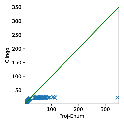
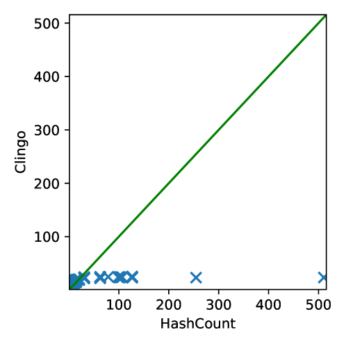
We present the TQP scores of $\mathsf{MinLB}$ alongside other tools in Section 5.1. This table indicates that $\mathsf{MinLB}$ achieves the lowest TQP scores. Among existing minimal model enumerators, clingo demonstrates the best performance in terms of TQP score. Additionally, in Figure 1, we graphically compare the lower bounds returned by $\mathsf{Proj\text{-}Enum}$ and $\mathsf{HashCount}$ against those returned by clingo. Here, a point $(x,y)$ indicates that, for an instance, the lower bounds returned by our prototypes and clingo are $2^{x}$ and $2^{y}$, respectively. For an instance, if the corresponding point resides below the diagonal line, it indicates that $\mathsf{Proj\text{-}Enum}$ ($\mathsf{HashCount}$, resp.) returns a better lower bound than clingo. These plots clearly illustrate that $\mathsf{Proj\text{-}Enum}$ and $\mathsf{HashCount}$ return better lower bounds compared to other existing minimal model enumerators.

clingo	ApproxASP	$\#\mathsf{MinModels}$	$\mathsf{MinLB}$ (our prototype)
6491	6379	7743	5599

Table 1: The TQP scores of $\mathsf{MinLB}$ and other tools on model counting benchmark.

(a) The lower bound returned by $\mathsf{Proj\text{-}Enum}$

(b) The lower bound returned by $\mathsf{HashCount}$

Figure 1: The lower bound of $\mathsf{Proj\text{-}Enum}$ and $\mathsf{HashCount}$ vis-a-vis the lower bound returned by clingo on minimal model counting benchmark. The axes are in log scale.

5.2 Performance on Minimal Generator Benchmark

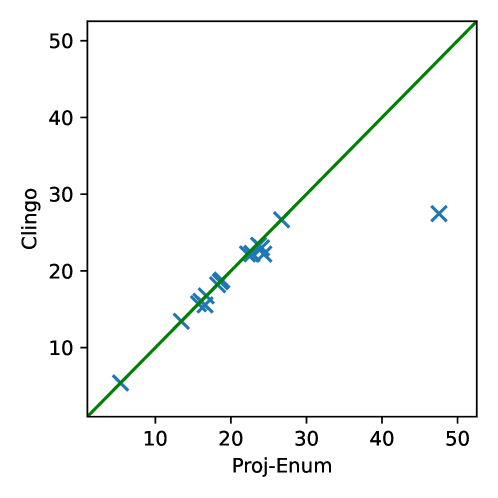
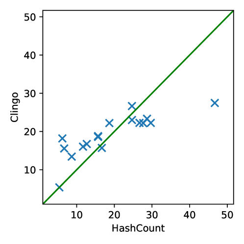
A.4 showcases the TQP scores of $\mathsf{MinLB}$ alongside other tools on the minimal generator benchmark. Notably, $\mathsf{HashCount}$ achieves the most favorable TQP scores on the benchmark. Additionally, Figure 2 graphically compares the lower bounds returned by $\mathsf{Proj\text{-}Enum}$ and $\mathsf{HashCount}$ against those computed by clingo.

clingo	ApproxASP	$\#\mathsf{MinModels}$	$\mathsf{MinLB}$ (our prototype)
6944	5713	9705	5043

Table 2: The TQP scores of $\mathsf{MinLB}$ and other tools on minimal generator benchmark.

(a) The lower bound returned by $\mathsf{Proj\text{-}Enum}$

(b) The lower bound returned by $\mathsf{HashCount}$

Figure 2: The lower bound returned by $\mathsf{Proj\text{-}Enum}$ and $\mathsf{HashCount}$ vis-a-vis the lower bound given by clingo on minimal generators benchmark. The axes are in log scale.

For a visual representation of the lower bounds returned by our $\mathsf{HashCount}$ and $\mathsf{Proj\text{-}Enum}$, we illustrate them graphically in Figure 3. In the plot, a point $(x,y)$ signifies that a tool returns a lower bound of at most $2^{y}$ for $x$ instances. The plot demonstrates that the lower bounds returned by $\mathsf{Proj\text{-}Enum}$ and $\mathsf{HashCount}$ surpass those of existing systems. The more experimental analysis is deferred to the appendix.

(a) Model counting benchmark

(b) Minimal generators benchmark

Figure 3: The lower bounds returned by $\mathsf{Proj\text{-}Enum}$, $\mathsf{HashCount}$, and existing minimal model counting tools. The $y$-axis show the log of the number of models.

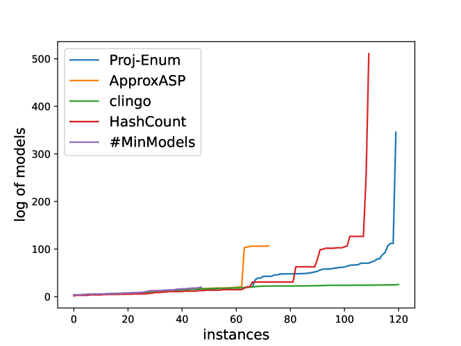
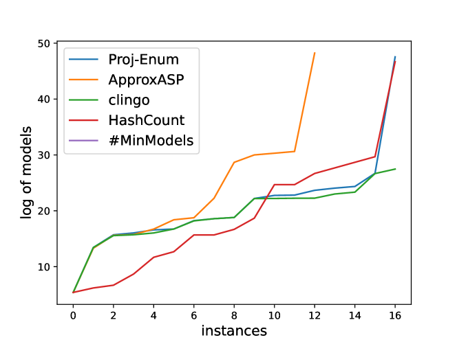
5.3 Another Performance Metric

To facilitate the comparison of lower bounds returned by two tools, we have introduced another metric for comparative analysis. If tools $A$ and $B$ yield lower bounds $C_{A}$ and $C_{B}$ respectively, their relative quality is defined in the following manner:

$$r_{AB}=\frac{1+\log{(C_{A}+1)}}{1+\log{(C_{B}+1)}}$$ (3)

If $r_{AB}>1$, then the lower bound returned by tool $A$ is superior to that of tool $B$.

In-depth Study on $\mathsf{Proj\text{-}Enum}$ and $\mathsf{HashCount}$

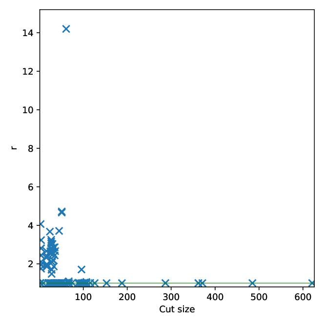
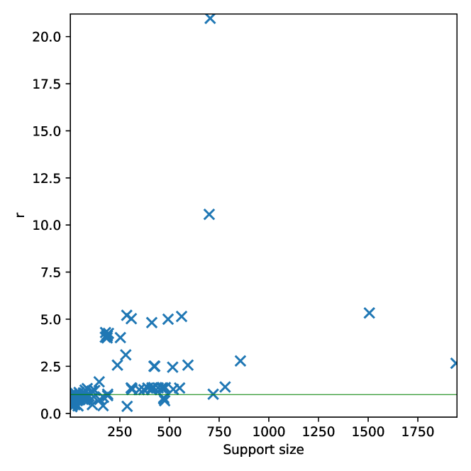
The performance of $\mathsf{Proj\text{-}Enum}$ and $\mathsf{HashCount}$ contingent upon the size of the cut and independent support, respectively. In this analysis, we explore the strengths and weaknesses of $\mathsf{Proj\text{-}Enum}$ and $\mathsf{HashCount}$ by measuring their relative quality, as defined in Equation 3, across various sizes of cuts and independent supports, respectively. This comparative analysis is visually represented in Figure 4, where clingo serves as the reference baseline.

In the graphical representations, each point $(x,y)$ corresponds to an instance where for the size of cut (independent support resp.) is $x$ and the prototype $\mathsf{Proj\text{-}Enum}$ ($\mathsf{HashCount}$ resp.) achieves a relative quality of $y$. A relative quality exceeding $1$ indicates that the lower bound returned by $\mathsf{Proj\text{-}Enum}$ or $\mathsf{HashCount}$ surpasses that of clingo. These plots reveal that $\mathsf{Proj\text{-}Enum}$ tends to perform well with smaller cut sizes, while $\mathsf{HashCount}$ demonstrates better performance across a range from small to medium sizes of independent support.

(a) The relative quality of $\mathsf{Proj\text{-}Enum}$ with varying cut size.

(b) The relative quality of $\mathsf{HashCount}$ with varying independent support size.

Figure 4: The relative quality of $\mathsf{Proj\text{-}Enum}$ and $\mathsf{HashCount}$ vis-a-vis different cut and independent support size, where clingo is used as the reference baseline. The horizontal line is drawn across $r=1$.

6 Conclusion

This paper introduces two innovative methods for computing a lower bound on the number of minimal models. Our first method, $\mathsf{Proj\text{-}Enum}$, leverages knowledge compilation techniques to provide improved lower bounds for easily decomposable formulas. The second method, $\mathsf{HashCount}$, utilizes recent advancements in ASP+XOR reasoning systems and demonstrates performance that varies with the size of the independent support. Our proposed methods exploit the expressive power of ASP semantics and robustness of well-engineered ASP systems. Looking forward, our research will focus on counting projected minimal models. We also plan to explore the counting of minimal correction subsets, which are closely related to minimal models.

Appendix

Appendix A Deferred Proofs of Section 2

Proof of Lemma 1

Proof A.2.

‘if’ part proof: Let $I=\{a\textprime_{1},\ldots,a\textprime_{k}\}\subseteq\mathcal{I}$ be a minimal generator of $D$ and $\mathcal{C}(I,D)=\{t\textprime_{1},\ldots,t\textprime_{m}\}$. We proof that $\sigma=\{p_{a\textprime_{1}},\ldots,p_{a\textprime_{k}},q_{t\textprime_{1}},\ldots,q_{t\textprime_{m}}\}$ is a minimal model of $\mathsf{MG}(D)$. By definition of $\mathsf{MG}(D)$, $\sigma$ is a model of $\mathsf{MG}(D)$. Now we show that $\sigma$ is a minimal model of $\mathsf{MG}(D)$. We proof it by contradiction and assume that there is model $\sigma\textprime\models\mathsf{MG}(D)$ and $\sigma\textprime$ is strictly smaller than $\sigma$. As $I$ is a minimal generator, there is no $I\textprime\subset I$ such that $\mathcal{C}(I,D)=\mathcal{C}(I\textprime,D)$. Thus, there is at least one $q_{t\textprime_{u}}\in\sigma\setminus\sigma\textprime$, i.e., $t\textprime_{u}\not\in\mathcal{C}(\sigma,D)$ and $t\textprime_{u}\in\mathcal{C}(\sigma\textprime,D)$. By definition of $\mathsf{MG}(D)$, $q_{t\textprime_{u}}$ occurs exactly in one clause of $\mathsf{MG}(G)$ and let us denote the clause by notation $C_{t\textprime_{u}}$. The literal $q_{t\textprime_{u}}$ is justified in minimal model $M$, thus $\forall a\in(\mathcal{I}\setminus I_{t\textprime_{u}}),p_{a}\not\in M$, which follows that the clause $C_{t\textprime_{u}}$ is not satisified by $\sigma\textprime$, which contradicts that $\sigma\textprime\models\mathsf{MG}(D)$.

‘only if’ part proof: Let $\sigma$ be a minimal model of $\mathsf{MG}(D)$ and assume that $I_{\sigma}=\{a|p_{a}\in\sigma\}$ is not a minimal generator of $D$ i.e., there is another $I\textprime_{\sigma}\subset I_{\sigma}$ such that $\mathcal{C}(I_{\sigma},D)=\mathcal{C}(I\textprime_{\sigma},D)$. By construction of $\mathsf{MG}(D)$, $\mathcal{C}(I_{\sigma},D)\subseteq\{q_{t}|q_{t}\in\sigma\}$. As $\sigma\in\mathsf{MinModels}(\mathsf{MG}(D))$, $\forall q_{t}\in\sigma$ has a justification. Note that the (positive) literal $q_{t}$ occurs in exactly one clause $\mathsf{MG}(D)$, which implies that $\forall a\in(\mathcal{I}\setminus I_{t}),p_{a}\not\in\sigma$. Thus, $\mathcal{C}(I_{\sigma},D)=\{q_{t}|q_{t}\in\sigma\}$, which follows that $\mathcal{C}(I\textprime_{\sigma},D)=\mathcal{C}(I_{\sigma},D)=\{q_{t}|q_{t}\in\sigma\}$. However, if $I\textprime_{\sigma}\subset I_{\sigma}$, then there are two possible cases: (i) either $\sigma\textprime=\{p_{a}|a\in I\textprime_{\sigma}\}\cup\{q_{t}|q_{t}\in\sigma\}\models\mathsf{MG}(D)$, that contradicts that $\sigma$ is a minimal model of $\mathsf{MG}(D)$, (ii) or $\sigma\textprime=\{p_{a}|a\in I\textprime_{\sigma}\}\cup\{q_{t}|q_{t}\in\sigma\}\not\models\mathsf{MG}(D)$ that contradicts that $\mathcal{C}(I_{\sigma},D)=\mathcal{C}(I\textprime_{\sigma},D)$.

Lemma A.3.

$\sigma\in\mathsf{MinModels}(F)$ if and only if $\sigma\in\mathsf{AS}(\mathcal{DLP}(F))$

Assume that $\sigma\in\mathsf{AS}(\mathcal{DLP}(F))$ but $\sigma\not\in\mathsf{MinModels}(F)$. As $\sigma\in\mathsf{AS}(\mathcal{DLP}(F))$, then $\sigma\models F$. Thus we only proof that there is no model $\sigma\textprime\subset\sigma$ such that $\sigma\textprime\models F$. For purpose of the contradiction, assume that there is a model $\sigma\textprime\subset\sigma$ and $\sigma\textprime\models F$. By consturction of program $\mathcal{DLP}(F)$, as $\sigma\textprime\models F$, $\sigma\textprime\models\mathcal{DLP}(F)$. Note that the reduct of $\mathcal{DLP}(F)$ w.r.t. $\sigma$ and $\sigma\textprime$ are same, more specifically, $\mathcal{DLP}(F)^{\sigma}=\mathcal{DLP}(F)^{\sigma\textprime}=\mathcal{DLP}(F)$ because there is no default negation in $\mathcal{DLP}(F)$. Thus, $\sigma\textprime\subset\sigma$ and $\sigma\textprime\models\mathcal{DLP}(F)^{\sigma}$, which contradicts that $\sigma$ is an answer set of $\mathcal{DLP}(F)$.

proof of “only if” part: The proof is trivial. If $\sigma\in\mathsf{MinModels}(F)$ and $\sigma\not\in\mathsf{AS}(\mathcal{DLP}(F))$, then there is another $\sigma\textprime\subset\sigma$ and $\sigma\textprime\models\mathcal{DLP}(F)$, which contradicts that $\sigma$ is a minimal model because $\sigma\textprime\models F$.

Appendix B Theoretical Analysis of $\mathsf{MinLB}$

Analysis of $\mathsf{Proj\text{-}Enum}$: Proof of Lemma 2

Proof B.5.

The proof consists on the following two parts:

1. for each $\sigma\in\mathsf{MinModels}(F)$, there is a sequence of $\sigma_{i}$, $i\in[1,k]$ such that $\sigma_{i}\in\mathsf{MinModels}(F)_{\downarrow V_{i}}$

2. for each $\sigma_{i}\in\mathsf{MinModels}(F)_{\downarrow V_{i}}$ and $i\in[1,k]$, then $\bigcup_{i}\sigma_{i}\in\mathsf{MinModels}(F)$

Proof of 1: Proof of this part is trivial. For each $\sigma\in\mathsf{MinModels}(F)$, it follows that $\sigma_{i}=\sigma_{\downarrow V_{i}}$.

Proof of 2: The variable set of each $\sigma_{i}$ is distinct or $\forall i\neq j,V_{i}\cap V_{j}=\emptyset$. For each $\sigma_{i}\in\mathsf{MinModels}(F)_{\downarrow V_{i}}$, there exists a $\sigma\in\mathsf{MinModels}(F)$, where $\sigma_{i}=\sigma_{\downarrow V_{i}}$. The $\bigcup_{i}\sigma_{i}$ assigns the variable of $V$ and the union of $\sigma_{i}$ or $\sigma=\bigcup_{i}\sigma_{i}$ is a minimal model of $F$

The correctness of Algorithm 1 can be established as follows:

Lemma B.6.

For Boolean formula $F$ and a cut $\mathcal{C}$, the minimal models of $F$ can be computed as follows: $\mathsf{MinModels}(F)=\bigcup_{\tau\in 2^{\mathcal{C}}}\mathsf{ProjMinModels}(F,\tau,\mathsf{Var}(F))$.

Proof B.7.

Lemma 2 demonstrates that minimal models can be computed through component decompositions. By taking the union over $\tau\in 2^{\mathcal{C}}$, we iterate over all possible assignments of $\mathcal{C}$. Consequently, $\mathsf{Proj\text{-}Enum}$ algorithm computes all minimal models of $F$ by conditioning over all possible assignments over $\mathcal{C}$. Therefore, the algorithm is correct.

Analysis of $\mathsf{HashCount}$.

We adopt the following notation: $s^{\star}=\log_{2}{|\mathsf{MinModels}(F)|}$. Each minimal model $\sigma$ of $F$ is an assignment over $\mathsf{Var}(F)$, and according to the definition of random XOR constraint (Gomes et al., 2006b ), $\sigma$ satisifies a random XOR constraint with probability of $\nicefrac{{1}}{{2}}$. Due to uniformity and randomness of XOR constraints, each minimal model of $F$ satisfies $m$ random and uniform XOR constraints with probability of $\nicefrac{{1}}{{2^{m}}}$. In our theoretical analysis, we apply the Markov inequality: if $Y$ is a non-negative random variable, then $\mathsf{Pr}[Y\geq a]\leq\frac{\mathbb{E}[Y]}{a}$, where $a>0$.

Lemma B.8.

For arbitrary $s$, $\mathsf{Pr}[|\mathsf{MinModels}(F^{s})\geq 1|]\leq\frac{2^{s^{\star}}}{2^{s}}$.

Proof B.9.

For each $\sigma\in\mathsf{MinModels}(F)$, we define a random variable $Y_{\sigma}\in\{0,1\}$ and $Y_{\sigma}=1$ indicates that $\sigma$ satisifies the first $s$ XOR constraints $Q^{1},\ldots,Q^{s}$, otherwise, $Y_{\sigma}=0$. The random variable $Y$ is the summation, $Y=\sum_{\sigma\in\mathsf{MinModels}(F)}Y_{\sigma}$. The expected value of $Y$ can be calculated as $\mathbb{E}(Y)=\sum_{\sigma\in\mathsf{MinModels}(F)}\mathbb{E}(Y_{\sigma})$.

Due to the nature of random and uniform XOR constraints, each minimal model $\sigma\in\mathsf{MinModels}(F)$ satisfies all $s$ XOR constraints with probability $\frac{1}{2^{s}}$. It follows that the expected value $\mathbb{E}(Y_{\sigma})=\frac{1}{2^{s}}$, and the expected value of $Y$ is $\mathbb{E}(Y)=\frac{|\mathsf{MinModels}(F)|}{2^{s}}=\frac{2^{s^{\star}}}{2^{s}}$. According to the Markov inequality:

$$\mathsf{Pr}[|\mathsf{MinModels}(F^{s})\geq 1|] \leq\frac{2^{s^{\star}}}{2^{s}}$$

Lemma B.10.

Given a formula $F$ and confidence $\delta$, if $\mathsf{\mathsf{HashCount}}(F,\delta)$ returns $2^{s-\alpha}$, then $\mathsf{Pr}[2^{s-\alpha}\leq|\mathsf{MinModels}(F)|]\geq 1-\delta$

Proof B.11.

Given a input Boolean formula $F$ and for each $m\in[1,|\mathcal{X}|-1]$, we denote the following two events: $I_{m}$ denotes the event that Algorithm 2 invokes $\mathsf{MinModels}(F^{m})$ and $E_{m}$ denotes the event that $|\mathsf{MinModels}(F^{m})|\geq 1$. The algorithm $\mathsf{\mathsf{HashCount}}(F,\delta)$ returns an incorrect bound when $s-\alpha>s^{\star}$ and let use the notation $\mathsf{Error}$ to denote that $\mathsf{\mathsf{HashCount}}(F,\delta)$ returns an incorrect bound or $\mathsf{\mathsf{HashCount}}(F,\delta)>2^{s^{\star}}$. The upper bound of $\mathsf{Pr}[\mathsf{Error}]$ can be calculated as follows:

$$\mathsf{Pr}[\mathsf{Error}] =\mathsf{Pr}[\text{$\mathsf{\mathsf{HashCount}}(F,\delta)$ returns $2^{s-\alpha}$ and }s>s^{\star}+\alpha]$$

$$\leq\sum_{s>s^{\star}+\alpha}\mathsf{Pr}[I_{s}\cap E_{s}]\leq\sum_{s>s^{\star}+\alpha}\mathsf{Pr}[E_{s}]$$

$$\leq\sum_{s>s^{\star}+\alpha}\mathsf{Pr}[|\mathsf{MinModels}(F^{s})|\geq 1]\leq\sum_{s>s^{\star}+\alpha}\frac{2^{s^{\star}}}{2^{s}}$$ According to Lemma B.8

$$\leq\frac{1}{2^{\alpha}}\times 2\leq 2^{1-\alpha}\leq 2^{\log_{2}{\delta}}\leq\delta$$

Thus, $\mathsf{Pr}[\text{$\mathsf{\mathsf{HashCount}}(F,\delta)$ returns $2^{s-\alpha}$ and }s\leq s^{\star}+\alpha]\geq 1-\delta$.

Analysis of Theorem 1

Proof B.12.

The proof consists of two cases.

(i) When $\mathsf{MinLB}$ calls $\mathsf{Proj\text{-}Enum}$ (if $|\mathcal{C}|\leq 50$). In the case, the proof follows Lemma B.6.

(ii) $\mathsf{MinLB}$ calls $\mathsf{HashCount}$. In the case, the proof follows Lemma B.10.

References

- Agrawal et al., (2021) Agrawal, D., Pote, Y., and Meel, K. S. Partition function estimation: A quantitative study. arXiv preprint arXiv:2105.11132 2021.
- Alrabbaa et al., (2018) Alrabbaa, C., Rudolph, S., and Schweizer, L. Faceted answer-set navigation. In RuleML+RR 2018, pp. 211–225. Springer.
- Alviano, (2017) Alviano, M. Model enumeration in propositional circumscription via unsatisfiable core analysis. TPLP, 17(5-6):708–725 2017.
- Alviano et al., (2022) Alviano, M., Dodaro, C., Fiorentino, S., Previti, A., and Ricca, F. Enumeration of minimal models and MUSes in WASP. In LPNMR 2022, pp. 29–42. Springer.
- Angiulli et al., (2014) Angiulli, F., Ben-Eliyahu, R., Fassetti, F., and Palopoli, L. On the tractability of minimal model computation for some CNF theories. Artificial Intelligence, 210:56–77 2014.
- Angiulli et al., (2022) Angiulli, F., Ben-Eliyahu, R., Fassetti, F., and Palopoli, L. Graph-based construction of minimal models. Artificial Intelligence, 313:103754 2022.
- Ben-Eliyahu, (2005) Ben-Eliyahu, R. An incremental algorithm for generating all minimal models. Artificial Intelligence, 169(1):1–22 2005.
- Ben-Eliyahu and Dechter, (1994) Ben-Eliyahu, R. and Dechter, R. Propositional semantics for disjunctive logic programs. Annals of Mathematics and Artificial intelligence, 12:53–87 1994.
- Ben-Eliyahu and Dechter, (1996) Ben-Eliyahu, R. and Dechter, R. On computing minimal models. Annals of Mathematics and Artificial Intelligence, 18(1):3–27 1996.
- Ben-Eliyahu and Palopoli, (1997) Ben-Eliyahu, R. and Palopoli, L. Reasoning with minimal models: Efficient algorithms and applications. Artificial Intelligence, 96(2):421–449 1997.
- Bozzano et al., (2022) Bozzano, M., Cimatti, A., Griggio, A., Jonáš, M., and Kimberly, G. Analysis of cyclic fault propagation via ASP. In LPNMR 2022, pp. 470–483. Springer.
- Brewka et al., (2015) Brewka, G., Delgrande, J., Romero, J., and Schaub, T. asprin: Customizing answer set preferences without a headache. In AAAI 2015, volume 29.
- (13) Cadoli, M. The complexity of model checking for circumscriptive formulae. Information Processing Letters, 44(3):113–118 1992a.
- (14) Cadoli, M. On the complexity of model finding for nonmonotonic propositional logics. In Italian Conference on Theoretical Computer Science 1992b, pp. 125–139.
- Chakraborty et al., (2013) Chakraborty, S., Meel, K. S., and Vardi, M. Y. A scalable approximate model counter. In CP 2013, pp. 200–216. Springer.
- Chakraborty et al., (2016) Chakraborty, S., Meel, K. S., and Vardi, M. Y. Algorithmic improvements in approximate counting for probabilistic inference: From linear to logarithmic SAT calls. In IJCAI 2016, pp. 3569–3576.
- Clark, (1978) Clark, K. L. Negation as failure. Logic and data bases, pp. 293–322 1978.
- Darwiche, (2004) Darwiche, A. New advances in compiling CNF to decomposable negation normal form. In ECAI 2004, pp. 328–332. Citeseer.
- De Kleer et al., (1992) De Kleer, J., Mackworth, A. K., and Reiter, R. Characterizing diagnoses and systems. Artificial intelligence, 56(2-3):197–222 1992.
- Durand and Hermann, (2008) Durand, A. and Hermann, M. On the counting complexity of propositional circumscription. Information Processing Letters, 106(4):164–170 2008.
- Eiter and Gottlob, (1993) Eiter, T. and Gottlob, G. Propositional circumscription and extended closed-world reasoning are -complete. Theoretical Computer Science, 114(2):231–245 1993.
- Faber et al., (2016) Faber, W., Vallati, M., Cerutti, F., and Giacomin, M. Solving set optimization problems by cardinality optimization with an application to argumentation 2016.
- Fichte et al., (2022) Fichte, J. K., Gaggl, S. A., and Rusovac, D. Rushing and strolling among answer sets–navigation made easy. In AAAI 2022, volume 36, pp. 5651–5659.
- Fichte et al., (2021) Fichte, J. K., Hecher, M., and Hamiti, F. The model counting competition 2020. Journal of Experimental Algorithmics (JEA), 26:1–26 2021.
- Gebser et al., (2013) Gebser, M., Kaufmann, B., Romero, J., Otero, R., Schaub, T., and Wanko, P. Domain-specific heuristics in answer set programming. In AAAI 2013, volume 27, pp. 350–356.
- Gebser et al., (2012) Gebser, M., Kaufmann, B., and Schaub, T. Conflict-driven answer set solving: From theory to practice. Artificial Intelligence, 187:52–89 2012.
- Gelfond and Lifschitz, (1991) Gelfond, M. and Lifschitz, V. Classical negation in logic programs and disjunctive databases. New generation computing, 9:365–385 1991.
- Gomes et al., (2007) Gomes, C. P., Hoffmann, J., Sabharwal, A., and Selman, B. From sampling to model counting. In IJCAI 2007, volume 2007, pp. 2293–2299.
- (29) Gomes, C. P., Sabharwal, A., and Selman, B. Model counting: A new strategy for obtaining good bounds. In AAAI 2006a, volume 10, pp. 1597538–1597548.
- (30) Gomes, C. P., Sabharwal, A., and Selman, B. Near-uniform sampling of combinatorial spaces using XOR constraints. NIPS, 19 2006b.
- Gomes et al., (2021) Gomes, C. P., Sabharwal, A., and Selman, B. Model counting. In Handbook of satisfiability 2021, pp. 993–1014. IOS press.
- Hamann and Strasser, (2018) Hamann, M. and Strasser, B. Graph bisection with pareto optimization. Journal of Experimental Algorithmics (JEA), 23:1–34 2018.
- Hunter et al., (2008) Hunter, A., Konieczny, S., and others. Measuring inconsistency through minimal inconsistent sets. KR, 8(358-366):42 2008.
- Jabbour et al., (2017) Jabbour, S., Sais, L., and Salhi, Y. Mining top-k motifs with a SAT-based framework. Artificial Intelligence, 244:30–47 2017.
- Jannach et al., (2016) Jannach, D., Schmitz, T., and Shchekotykhin, K. Parallel model-based diagnosis on multi-core computers. JAIR, 55:835–887 2016.
- Kabir et al., (2024) Kabir, M., Chakraborty, S., and Meel, K. S. Exact ASP counting with compact encodings. In AAAI 2024, volume 38, pp. 10571–10580.
- Kabir et al., (2022) Kabir, M., Everardo, F. O., Shukla, A. K., Hecher, M., Fichte, J. K., and Meel, K. S. ApproxASP–a scalable approximate answer set counter. In AAAI 2022, volume 36, pp. 5755–5764.
- Kabir and Meel, (2023) Kabir, M. and Meel, K. S. A fast and accurate ASP counting based network reliability estimator. In LPAR 2023, pp. 270–287.
- Kirousis and Kolaitis, (2003) Kirousis, L. M. and Kolaitis, P. G. The complexity of minimal satisfiability problems. Information and Computation, 187(1):20–39 2003.
- Korhonen and Järvisalo, (2021) Korhonen, T. and Järvisalo, M. Integrating tree decompositions into decision heuristics of propositional model counters. In CP 2021, pp. 8–1.
- Lagniez and Marquis, (2017) Lagniez, J.-M. and Marquis, P. An improved Decision-DNNF compiler. In IJCAI 2017, volume 17, pp. 667–673.
- Lee and Lin, (2006) Lee, J. and Lin, F. Loop formulas for circumscription. Artificial Intelligence, 170(2):160–185 2006.
- Li et al., (2021) Li, Z., Yisong, W., Zhongtao, X., and Renyan, F. Computing propositional minimal models: MiniSAT-based approaches. Journal of Computer Research and Development, 58(11):2515–2523 2021.
- Liffiton and Sakallah, (2008) Liffiton, M. H. and Sakallah, K. A. Algorithms for computing minimal unsatisfiable subsets of constraints. Journal of Automated Reasoning, 40:1–33 2008.
- Lifschitz, (1985) Lifschitz, V. Computing circumscription. In IJCAI 1985, volume 85, pp. 121–127.
- Marek and Truszczyński, (1999) Marek, V. W. and Truszczyński, M. Stable models and an alternative logic programming paradigm. The Logic Programming Paradigm: a 25-Year Perspective, pp. 375–398 1999.
- Marques-Silva et al., (2013) Marques-Silva, J., Heras, F., Janota, M., Previti, A., and Belov, A. On computing minimal correction subsets. In IJCAI 2013.
- McCarthy, (1980) McCarthy, J. Circumscription—a form of non-monotonic reasoning. Artificial intelligence, 13(1-2):27–39 1980.
- Mencía et al., (2015) Mencía, C., Previti, A., and Marques-Silva, J. Literal-based MCS extraction. In IJCAI 2015.
- Minker, (1982) Minker, J. On indefinite databases and the closed world assumption. In CADE 1982, pp. 292–308. Springer.
- Padoa, (1901) Padoa, A. Essai d’une théorie algébrique des nombres entiers, précédé d’une introduction logique à une théorie déductive quelconque. Bibliothèque du Congrès International de Philosophie, 3:309–365 1901.
- Reiter, (1980) Reiter, R. A logic for default reasoning. Artificial intelligence, 13(1-2):81–132 1980.
- Salhi, (2019) Salhi, Y. On enumerating all the minimal models for particular CNF formula classes. In ICAART (2) 2019, pp. 403–410.
- Soos et al., (2020) Soos, M., Gocht, S., and Meel, K. S. Tinted, detached, and lazy CNF-XOR solving and its applications to counting and sampling. In CAV 2020, pp. 463–484. Springer.
- Soos and Meel, (2022) Soos, M. and Meel, K. S. Arjun: An efficient independent support computation technique and its applications to counting and sampling. In ICCAD 2022, pp. 1–9.
- Thimm, (2016) Thimm, M. On the expressivity of inconsistency measures. Artificial Intelligence, 234:120–151 2016.
- Thurley, (2006) Thurley, M. sharpSAT–counting models with advanced component caching and implicit BCP. In SAT 2006, pp. 424–429. Springer.