Active Learning for Derivative-Based Global Sensitivity Analysis with Gaussian Processes

Abstract

We consider the problem of active learning for global sensitivity analysis of expensive black-box functions. Our aim is to efficiently learn the importance of different input variables, e.g., in vehicle safety experimentation, we study the impact of the thickness of various components on safety objectives. Since function evaluations are expensive, we use active learning to prioritize experimental resources where they yield the most value. We propose novel active learning acquisition functions that directly target key quantities of derivative-based global sensitivity measures (DGSMs) under Gaussian process surrogate models. We showcase the first application of active learning directly to DGSMs, and develop tractable uncertainty reduction and information gain acquisition functions for these measures. Through comprehensive evaluation on synthetic and real-world problems, our study demonstrates how these active learning acquisition strategies substantially enhance the sample efficiency of DGSM estimation, particularly with limited evaluation budgets. Our work paves the way for more efficient and accurate sensitivity analysis in various scientific and engineering applications.

1 Introduction

Sensitivity analysis is the study of how variation and changes in the output of a function can be attributed to distinct sources of variability in the function inputs Iooss and Saltelli [2017]. More precisely, we seek to determine how changes in each input variable impact the output. Sensitivity analysis can be used for several purposes, including identifying the input variables that are most influential for the function output and those that are least influential [Iooss and Saltelli, 2017], and quantifying variable importance in order to explore and interpret a model’s behavior [Van Stein et al., 2022]. Sensitivity analysis is an important tool in many fields of science and engineering to understand complex, often black-box systems. It has proven particularly important for environmental modeling [Razavi and Gupta, 2015, Wagener and Pianosi, 2019], geosciences [Wainwright et al., 2014, Ciriello et al., 2019], chemical engineering [Sepúlveda et al., 2014], biology [Kiparissides et al., 2009], engineering safety experimentation [Qian et al., 2019], and other simulation-heavy domains. In these settings, function evaluations often involve time-consuming simulations or costly lab experiments, so it is important to perform the sensitivity analysis with as few function evaluations as possible. For example, sensitivity analysis is widely applicable in environmental modeling, particularly in climate change research. It helps to understand how various parameters—such as CO₂ emissions, temperature increases, or deforestation rates—influence the output of climate models. By identifying which variables most directly impact model outcomes, researchers can better prioritize efforts in data collection, model refinement, and policy development [Razavi and Gupta, 2015].

Sensitivity analysis can be either local or global. Local sensitivity analysis (LSA) [Gustafson et al., 1996] studies the effect of perturbations of single input variables at a fixed, nominal point. Input sensitivity is measured only locally to that nominal point and does not take into account any interactions. Global sensitivity analysis (GSA) [Saltelli et al., 2008], on the other hand, evaluates sensitivity over an entire compact input space and includes measures of interactions between the various input dimensions. Here, we focus on GSA.

Approaches for GSA can be categorized into two main types: variance-based measures, also referred to as ANOVA decomposition or Sobol methods [Prieur and Tarantola, 2017], and derivative-based global sensitivity measures (DGSMs) [Kucherenko and Iooss, 2014]. Variance-based measures quantify the importance of different input variables based on their contribution to the global variability of the function output. In contrast, DGSMs quantify importance based on the global variability of the function’s gradient. They are defined as an integral over the gradients or a function of the gradients.

DGSMs can often be computed directly from the function. However, for expensive black-box functions, integrating a function of the gradients across the input space is infeasible due to the limited number of function evaluations or a lack of gradient information. In this case, the function is modeled by a surrogate Gaussian process (GP) [De Lozzo and Marrel, 2016], which allows for tractable computation of both the function surrogate and its gradient. Previous work [De Lozzo and Marrel, 2016, Kucherenko and Iooss, 2014, Le Gratiet et al., 2017] used random and quasirandom sequences to select the data points for learning the GP; however, these space-filling approaches still require a substantial number of evaluations to accurately estimate the DGSMs. In this work, we propose several active learning acquisition functions for efficient estimation of the DGSMs.

We show here that DGSMs can be targeted for active learning with information-based acquisition functions that are tractable under GP surrogate models, which are standard for GSA. Applying active learning to DGSM quantities (e.g., gradient, absolute value of the gradient, squared value of the gradient) allows for sensitivity analysis to be performed in a highly sample-efficient manner, suitable for engineering and science applications with small evaluation budgets. To the best of our knowledge, this is the first study proposing active learning acquisition functions directly targeting the DGSM measures. It is also the first work to empirically study the impact of different strategies on DGSMs under a limited budget, including general acquisition functions targeting the function such as variance and information gain maximization strategies [Krause et al., 2008].

Figure 1: (Left) Posteriors of $f$, $df/dx$, and $(df/dx)^{2}$ are computed from a GP surrogate given six observations of $f$ (black dots). Posteriors are shown as posterior mean (line) and 95% credible interval (shaded). (Right) Acquisition functions are computed from these posteriors, targeting $f$ and derivative sensitivity measures. Dotted vertical lines show the maximizer. Acquisition functions that directly target DGSMs, not just $f$ generally, are required to learn the DGSMs efficiently.

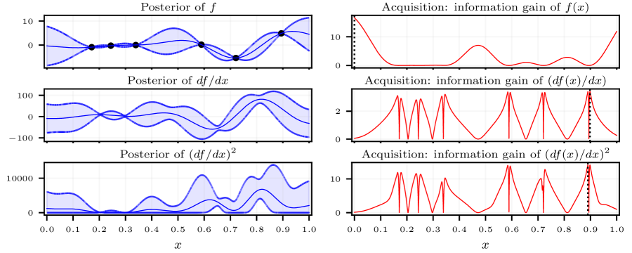
To illustrate the utility of the proposed acquisition functions, we consider active learning using the classic Forrester [Forrester et al., 2008] test function (Fig. 1). The posteriors of $f$ and $df/dx$ given observations of $f$ are computed from the GP (Sections 2.4 and 2.5). The posterior of $(df/dx)^{2}$ is computed from that of $df/dx$ (Section 4.4); the squared DGSM is the integral of that function (Section 2.3). Two acquisition functions show the value of evaluating any particular point under different targets: one quantifies the information gain of the function generally (BALD, Section 3), and the other quantifies the information gain of the squared derivative (Section 4.4). The acquisition functions illustrate why active learning strategies that only target learning $f$ are not effective for learning DGSMs. In particular, to learn $f$, active learning selects points that are far from existing observations, where $f$ is most uncertain. To learn the squared DGSM, active learning selects points that are adjacent to existing observations, as that adjacency is valuable for the derivative estimate.

The contributions of this paper are:

• We introduce the first active learning methods to directly target the quantities used for derivative-based global sensitivity analysis, namely, the gradient, its absolute value, and its square.

• We propose acquisition functions based on uncertainty reduction and information gain, and we show how to tractably compute the information gain for DGSMs using GP models.

• With a thorough evaluation on synthetic and real-world problems, we show that active learning substantially accelerates GSA in settings with limited evaluation budgets. The implementation for our methods, the baselines, and the synthetic and real-world problems is available in our code (https://github.com/belakaria/AL-GSA-DGSMs)

2 Background

In this section, we define the problem and provide a review of DGSMs, GPs, and their derivatives. For a thorough review of GSA, see Iooss and Saltelli [2017].

2.1 Problem Setup

We wish to analyze the sensitivity of a black-box function defined over a compact $d$-dimensional input space $\mathcal{X}$. We suppose that evaluating $f$ at any particular input $\mathbf{x}\in\mathcal{X}$, that is, observing $y=f(\mathbf{x})+\epsilon$ with $\epsilon$ the observation noise, is expensive. The ground-truth sensitivity measure, which we denote as $S(f,\mathcal{X})$, has a $d$-dimensional output that provides a sensitivity measure for each input dimension $x_{i}$, $i=1,\ldots,d$. We estimate $S$ by making $t$ observations of $f$, for which we denote with $X=[\mathbf{x}_{1},\dots,\mathbf{x}_{t}]$ the set of observed inputs, $Y=[y_{1},\dots,y_{t}]$ the function evaluations at those inputs, and $\mathcal{D}=\{X,Y\}$ the full observed data. We learn a surrogate model of $f$ from $\mathcal{D}$ and then evaluate $S$ on a surrogate for $f$. Here, we will denote the surrogate as $\hat{f}$; in practice, we will use the GP posterior mean $\hat{f}(\mathbf{x})=\mu(\mathbf{x})$, which we introduce in Section 2.4. Given the surrogate, we estimate $\hat{S}(f,\mathcal{X}|\mathcal{D})=S(\hat{f},\mathcal{X})$.

Our active learning problem is to select the input locations $X$ so that $\hat{S}$ provides the best estimate of the true global measure $S$. We do so sequentially with a budget of $T$ total evaluations. Generally, $\hat{S}$ will better approximate $S$, as the surrogate $\hat{f}$ better approximates $f$. However, when $T$ is small, it is important to consider the particular form of $S$ to design the most effective strategy, as opposed to simply trying to learn a good global surrogate. Here, we develop strategies tailored for $S$ being a DGSM. We introduce DGSMs in Section 2.3, and in Section 4 develop the acquisition strategies.

2.2 Bayesian Active Learning

The methods we develop here are cast as Bayesian active learning algorithms. Bayesian active learning is a flexible framework that combines Bayesian inference principles with active learning strategies, where data points are sequentially selected in a sample-efficient manner Houlsby et al. [2011]. In this work, the Bayesian active learning algorithm iterates through three steps. First, at iteration $t$, we build the GP surrogate model based on the evaluated data points. Second, we use an acquisition function to score the utility of unevaluated inputs using the GP posterior. The acquisition function will generally guide the input space exploration while attempting to learn the target quantities. We select the input with the highest acquisition value. Third, we evaluate the black-box function on the selected input and augment $\mathcal{D}$ with the new observation. We summarize the process in Algorithm 1. In Section 4, we develop acquisition functions, $\alpha(\cdot)$, that are tailored to learning DGSMs.

Algorithm 1 Bayesian Active Learning

Input: $\mathcal{X}$, $f(\mathbf{x})$, surrogate model $\mathcal{GP}$, utility function $\alpha(\mathbf{x},\mathcal{GP})$, total budget $T$.
Output: $\mathcal{D}_{T},\mathcal{GP}$.

1:  Initialize data $\mathcal{D}_{0}$ with $T_{0}$ starting observations.

2:  for each iteration $t\in[T_{0},T]$ do

3:     Fit the surrogate model $\mathcal{GP}(\mathcal{D}_{t-1})$ using $\mathcal{D}_{t-1}$ .

4:     Select the next input for evaluation by maximizing the acquisition function,$\mathbf{x}^{*}\leftarrow\arg\max_{\mathbf{x}\in\mathcal{X}}\alpha(\mathbf{x},\mathcal{GP}(\mathcal{D}_{t-1}))$.

5:     Evaluate the black-box function to observe $y^{*}=f(\mathbf{x}^{*})$.

6:     Update data $\mathcal{D}_{t}=\mathcal{D}_{t-1}\cup\{(\mathbf{x^{*}},y^{*})\}$.

7:  end for

2.3 Derivative-based Global Sensitivity Measures (DGSMs)

In this section, we provide the background and definitions for our target sensitivity measures, DGSMs. DGSMs are defined as the integral over the input space of a function of the derivative of the black-box function. There are three widely-used gradient functions in DGSMs: the raw gradient, the absolute value of the gradient, and the square of the gradient Kucherenko et al. [2009]:

$$S_{R}(f,\mathcal{X})_{i}=\frac{1}{|\mathcal{X}|}\int_{\mathcal{X}}\left(\frac{\partial f(\mathbf{x})}{\partial x_{i}}\right)d\mathbf{x},$$

$$S_{Ab}(f,\mathcal{X})_{i}=\frac{1}{|\mathcal{X}|}\int_{\mathcal{X}}\left|\frac{\partial f(\mathbf{x})}{\partial x_{i}}\right|d\mathbf{x},$$

$$S_{Sq}(f,\mathcal{X})_{i}=\frac{1}{|\mathcal{X}|}\int_{\mathcal{X}}\left(\frac{\partial f(\mathbf{x})}{\partial x_{i}}\right)^{2}d\mathbf{x}.$$

In the remainder of the paper, we will refer to these quantities as the raw DGSM, absolute DGSM, and squared DGSM. These quantities may also be defined with non-uniform densities on $\mathcal{X}$.

For the purpose of evaluating input sensitivity, the raw DGSM is considered unstable and uninformative due to a phenomenon known as the cancellation effect. In nonmonotonic functions, positive parts of the gradient cancel out negative parts of the gradient when integrated over the entire input space, leading to a small value for the raw DGSM even for important dimensions. The most commonly used DGSMs in practice are the absolute and squared DGSMs, which avoid the cancellation effect. The squared DGSM is especially popular because of its connection to the variance of the gradient Kucherenko and Iooss [2014]. Computing DGSMs requires computing a $d$-dimensional integral over $\mathcal{X}$. This integration is usually done via Monte Carlo (MC) or quasi-Monte Carlo (QMC) sampling [Dick et al., 2013].

2.4 GP Surrogates for Sensitivity Analysis

When function evaluations are expensive, the integrals over the input space required to compute the DGSMs may not be evaluated tractably from $f$. Moreover, if $f$ is black-box, we do not always have access to its gradients. Both of these issues can be avoided by using a surrogate function for $f$.

GSA of expensive, black-box functions is usually done using a GP surrogate model [De Lozzo and Marrel, 2016]. GPs are characterized by a mean function $m:\mathcal{X}\rightarrow\mathbb{R}$ and a kernel function covariance $\mathcal{K}:\mathcal{X}\times\mathcal{X}\rightarrow\mathbb{R}$. A GP prior for the function, $f\sim\mathcal{GP}(m,\mathcal{K})$, means that the function values at any finite set of inputs are jointly normally distributed. For any input $\mathbf{x}_{*}\in\mathcal{X}$, the function value at that input has a normally-distributed posterior $f(\mathbf{x}_{*})|\mathcal{D}\sim\mathcal{N}(\mu_{*},\sigma_{*}^{2})$, whose predictive mean and variance are defined as:

$$\mu_{*}=\mathcal{K}_{\mathbf{x}_{*},X}K_{\mathcal{D}}^{-1}(Y-m_{X})+m_{\mathbf{x}_{*}},~{}~{}~{}\sigma^{2}_{*}=\mathcal{K}_{\mathbf{x}_{*},\mathbf{x}_{*}}-\mathcal{K}_{\mathbf{x}_{*},X}K_{\mathcal{D}}^{-1}\mathcal{K}_{X,\mathbf{x}_{*}},$$

where $\mathcal{K}_{\mathbf{x}_{*},\mathbf{x}_{*}}=\mathcal{K}(\mathbf{x}_{*},\mathbf{x}_{*})$, $\mathcal{K}_{\mathbf{x}_{*},X}=[\mathcal{K}(\mathbf{x}_{*},\mathbf{x}_{j})]_{j=1}^{t}$, $m_{\mathbf{x}}=m(\mathbf{x})$, and $K_{\mathcal{D}}=\mathcal{K}_{X,X}+\eta^{2}I$, with $\mathcal{K}_{X,X}=\mathcal{K}(X,X)$ and $\eta^{2}$ the observation noise variance of $y$ [Rasmussen and Williams, 2006]. We introduce the short-hand notation $\mu_{*}:=\mu(\mathbf{x}_{*})$ and $\sigma^{2}_{*}:=\sigma(\mathbf{x}_{*})^{2}$ for the posterior mean and variance functions.

GPs are differentiable when using any twice-differentiable kernel function $\mathcal{K}$ and a differentiable mean function $m$. The gradient of the GP provides a tractable estimate of the gradient of the expensive black-box function $f$ under commonly-used kernels (e.g., RBF). DGSMs can then be computed in a fast and scalable way on the posterior of $f$ [De Lozzo and Marrel, 2016].

2.5 Derivatives of Gaussian Processes

GPs are closed under linear operations, therefore the derivative of a GP is itself a GP [Rasmussen and Williams, 2006]. This enables us to derive an analytical distribution for the surrogate model’s gradient. Since $f$ is defined over a $d$-dimensional input space, the model’s gradient has a $d$-dimensional output. Under a GP prior, the joint distribution between (potentially noisy) observations of $f$ and the gradient of $f$ at a new point $\mathbf{x}_{*}$ is as follows Rasmussen and Williams [2006]:

$$\begin{bmatrix}Y\\ \nabla f(\mathbf{x}_{*})\end{bmatrix}\sim\mathcal{N}\left(\begin{bmatrix}m_{X}\\ \nabla m_{\mathbf{x}_{*}}\end{bmatrix},\begin{bmatrix}K_{\mathcal{D}}&\nabla_{\mathbf{x}_{*}}\mathcal{K}_{X,\mathbf{x}_{*}}\\ \nabla_{\mathbf{x}_{*}}\mathcal{K}_{\mathbf{x}_{*},X}&\nabla^{2}_{\mathbf{x}_{*}}\mathcal{K}_{\mathbf{x}_{*},\mathbf{x}_{*}}\end{bmatrix}\right).$$

Given the observed data $\mathcal{D}$ as before, the gradient at $\mathbf{x}_{*}$ has a multivariate normal distribution: $\nabla f(\mathbf{x}_{*})|\mathcal{D}\sim\mathcal{N}(\mu^{\prime}_{*},\Sigma^{\prime}_{*})$, where

$$\mu^{\prime}_{*} =\nabla m_{\mathbf{x}_{*}}+\nabla_{\mathbf{x}_{*}}\mathcal{K}_{\mathbf{x}_{*},X}K_{\mathcal{D}}^{-1}(Y-m_{X}),$$ (1)

$$\Sigma^{\prime}_{*} =\nabla^{2}_{\mathbf{x}_{*}}\mathcal{K}_{\mathbf{x}_{*},\mathbf{x}_{*}}-\nabla_{\mathbf{x}_{*}}\mathcal{K}_{\mathbf{x}_{*},X}K_{\mathcal{D}}^{-1}\nabla_{\mathbf{x}_{*}}\mathcal{K}_{X,\mathbf{x}_{*}}.$$ (2)

Here, $\mu^{\prime}_{*}=\mu^{\prime}(\mathbf{x}_{*})$ and $\Sigma^{\prime}_{*}=\Sigma^{\prime}(\mathbf{x}_{*})$ are shorthand for the posterior mean and covariance functions of the gradient. Note that the posterior for the derivative may be obtained from observations only of $f$, and does not require direct observations of the derivative. The greatest computational expense in computing the GP posterior is the matrix inversion in $K_{\mathcal{D}}^{-1}$, which has complexity $\mathcal{O}(t^{3})$. This same term is also the most expensive term in the posterior for the derivative. Consequently, once the posterior of the GP has been computed, the computation of the derivative does not increase the overall complexity. Given the posterior of the derivative, the DGSMs are estimated by substituting the gradient of the function with the predictive mean of the gradient (Equation 1).

3 Related Work

The GP surrogate allows for computing DGSMs with a limited set of function evaluations. However, in budget-restricted experiments, the GP will only provide a faithful representation of the sensitivity of $f$ if the right set of inputs are evaluated. There has been limited work on efficiently selecting the inputs that lead to accurate DGSM estimation, particularly with a limited evaluation budget.

Random and space-filling designs: The most common approach for estimating DGSMs with a GP is to evaluate the function on either a random set of inputs or with a space-filling design. For the latter, quasirandom sequences like scrambled Sobol sequences [Owen, 1998] and Latin hypercube sampling [McKay et al., 1979] are two common choices. Space-filling designs are effective for GSA with a sufficiently large evaluation budget, however, as we will see below, they fail when the budget is limited.

General uncertainty reduction methods: Several Bayesian active learning approaches have been developed for the purpose of reducing global uncertainty about $f$. Information-based strategies that select the point that produces the largest information gain about a function’s outputs are popular and effective for global identification of $f$ [Shewry and Wynn, 1987, Krause et al., 2008, Houlsby et al., 2011]. Other global active learning approaches are based on variance reduction [Schein and Ungar, 2007] and expected improvement (EI) [Lam and Notz, 2008]. These general-purpose active learning strategies have been applied to the GSA problem. Pfingsten [2006] used global predictive variance reduction as the active learning target for the purpose of GSA; Chauhan et al. [2024] applied the EI criterion to GSA. These approaches are designed to generally minimize uncertainty of $f$, and do not specifically target improvement of any particular GSA measure. Acquisition functions that target $f$ are not sufficient to learn the DGSMs efficiently on a budget (Figure 1).

Active learning involving derivatives: Some work has incorporated derivatives into active learning for problems unrelated to GSA. Salem et al. [2019] and Spagnol et al. [2019] use sensitivity measures to eliminate variables during Bayesian optimization. Erickson et al. [2018] and Marmin et al. [2018] include a derivative term in an acquisition function for learning non-stationary functions. Wycoff et al. [2021] do active subspace identification with an acquisition function targeting the outer product of the gradient. See Appendix for further discussion and an empirical comparison to these methods.

Active learning for GSA: There has been limited work on applying active learning to GSA measures. Existing work considers only the Sobol index (variance-based measures). Le Gratiet et al. [2014] applied variance reduction directly to the Sobol index. However, this could not be done in closed form and required expensive simulations within each active learning step. More recently, Chauhan et al. [2024] developed an analytic improvement criterion that targets the numerator of the Sobol index. In this work, we propose the first active learning acquisition functions directly targeting DGSMs.

4 Bayesian Active Learning for Derivative-Based Sensitivity Analysis

In this section, we provide the expressions and details of the active learning acquisition functions that we propose to target the DGSM measures. We derive acquisition functions following three general strategies. The maximum variance acquisition functions select the point with the largest posterior variance in the quantity of interest, indicating the point with the most uncertainty. The variance reduction acquisition functions measure how much an observation at a point will reduce the variance at that point in expectation over the possible outcomes of the observation. Finally, the information gain acquisition functions quantify the expected reduction in entropy of the posterior of the quantity of interest for each point. The latter two strategies require computing the look-ahead distribution for the derivative, which we introduce in Section 4.1. We additionally discuss global look-ahead acquisition functions that measure the impact of input on the posterior across the entire input space.

4.1 The Derivative Look-Ahead Distribution

Effective active learning often relies on computing look-ahead distributions that predict the impact that making a particular observation will have on the model. For our purposes, we wish to predict the impact that observing $f$ at a candidate point $\mathbf{x}_{*}$ will have on the model’s derivatives at that location. This will allow us to select a point $\mathbf{x}_{*}$ that most improves the posterior of the derivatives, in expectation. Under a GP, this look-ahead distribution is tractable. Conditioned on the observations $\mathcal{D}$, $f(\mathbf{x}_{*})$ and $\frac{\partial f(\mathbf{x}_{*})}{\partial x_{i}}$ have a bivariate normal joint distribution for each input dimension $i$. The well-known formula for bivariate normal conditioning then provides the look-ahead distribution Lyu et al. [2021]: $\frac{\partial f(\mathbf{x}_{*})}{\partial x_{i}}\biggm{\lvert}f(\mathbf{x}_{*})=y_{*},\mathcal{D}\sim\mathcal{N}\left(\mu_{*,i}^{\prime\ell},(\sigma_{*,i}^{\prime\ell})^{2}\right)$, where the look-ahead mean and variance are

$$\mu_{*,i}^{\prime\ell}=\mu^{\prime}_{*,i}+\frac{\tilde{\sigma}_{*,i}}{\sigma_{*}^{2}}(y_{*}-\mu_{*}),~{}~{}~{}~{}~{}(\sigma_{*,i}^{\prime\ell})^{2}=(\sigma^{\prime}_{*,i})^{2}-\left(\frac{\tilde{\sigma}_{*,i}}{\sigma_{*}}\right)^{2},$$ (3)

with $\tilde{\sigma}_{*,i}=\textrm{Cov}[f(\mathbf{x}_{*}),\frac{\partial f(\mathbf{x}_{*})}{\partial x_{i}}|\mathcal{D}]$ the posterior covariance between $f$, and the derivative at $\mathbf{x}_{*}$, and $(\sigma^{\prime}_{*,i})^{2}=\sigma^{\prime}_{i}(\mathbf{x}_{*})^{2}=\left[\Sigma^{\prime}(\mathbf{x}_{*})\right]_{ii}$ the posterior variance of the derivative. As before, we use the notational short-hand $\sigma_{*,i}^{\prime\ell}=\sigma_{i}^{\prime\ell}(\mathbf{x}_{*})$ and $\mu_{*,i}^{\prime\ell}=\mu_{i}^{\prime\ell}(\mathbf{x}_{*})$. This result holds when $y_{*}$ is a noisy observation by replacing $\sigma_{*}^{2}$ with $\eta^{2}+\sigma_{*}^{2}$. Remarkably, the look-ahead variance is independent of the actual observed $y_{*}$, so acquisition functions that are based on the future variance of the derivative can be computed exactly in closed form. In the Appendix, we provide the look-ahead posterior distribution of the derivative of $f$ at any point in the input space after observing $f$ at $\mathbf{x}_{*}$.

4.2 Gradient Acquisition Functions

Maximum variance.

The posterior variance of each derivative is given in (Equation 2). The maximum derivative variance acquisition function uses the sum of the variances across dimensions to find points with high total uncertainty in the derivatives:

$$\alpha_{\textrm{{dv}{}}}(\mathbf{x})=\sum_{i=1}^{d}\sigma^{\prime}_{i}(\mathbf{x})^{2}.$$ (4)

Variance reduction.

The derivative variance reduction acquisition computes the expected reduction in variance of the derivatives produced by making an observation of $f$ at $\mathbf{x}$:

$$\alpha_{\textrm{{d}{v}\textsubscript{r}{}}}(\mathbf{x})=\sum_{i=1}^{d}\sigma_{i}^{\prime}(\mathbf{x})^{2}-\mathbb{E}_{y}[\sigma_{i}^{\prime\ell}(\mathbf{x})^{2}]=\sum_{i=1}^{d}\sigma_{i}^{\prime}(\mathbf{x})^{2}-\hat{\sigma}_{i}^{\prime\ell}(\mathbf{x})^{2},$$

where $\sigma_{i}^{\prime\ell}(\mathbf{x})^{2}$ is the look-ahead variance of the derivative (Equation 3). The expectation is dropped because the look-ahead variance is independent of the observed $y$ at the candidate point.

Information gain.

We express our derivative information gain acquisition function as the sum of information gains for each derivative. Let $H^{\prime}_{i}(\mathbf{x})=h\left(\frac{\partial f(\mathbf{x})}{\partial x_{i}}\big{\lvert}\mathcal{D}\right)$ be the differential entropy of each derivative posterior. The Gaussian entropy is well-known [Cover, 1999], and independent of $y$, yielding as the information gain:

$$\alpha_{\textrm{{dig}{}}}(\mathbf{x}) =\sum_{i=1}^{d}H^{\prime}_{i}(\mathbf{x})-\mathbb{E}_{y}\left[H^{\prime}_{i}(\mathbf{x}|f(\mathbf{x})=y\right)]=\frac{1}{2}\sum_{i=1}^{d}\log(2\pi\sigma_{i}^{\prime}(\mathbf{x})^{2})-\log(2\pi\sigma_{i}^{\prime\ell}(\mathbf{x})^{2}).$$

4.3 Absolute Gradient Acquisition Functions

Maximum variance.

The absolute value of a normal distribution is the folded normal distribution [Tsagris et al., 2014], whose mean and variance, $\mu_{i_{Ab}}^{\prime}(\mathbf{x})$ and $\sigma_{i_{Ab}}^{\prime}(\mathbf{x})^{2}$, are analytical and can be computed from the moments of the corresponding normal distribution. Using those results, the posterior of $\big{\lvert}\frac{\partial f(\mathbf{x})}{\partial x_{i}}\big{\lvert}$ has mean and variance:

$$\mu_{i_{Ab}}^{\prime}(\mathbf{x})=\sqrt{\frac{2}{\pi}}\sigma_{i}^{\prime}(\mathbf{x})e^{-\frac{1}{2}r^{2}_{i}(\mathbf{x})}+\mu_{i}^{\prime}(\mathbf{x})\left(1-2\Phi(-r_{i}(\mathbf{x}))\right),$$

$$\sigma_{i_{Ab}}^{\prime}(\mathbf{x})^{2}=\mu_{i}^{\prime}(\mathbf{x})^{2}+\sigma_{i}^{\prime}(\mathbf{x})^{2}-\mu_{i_{Ab}}^{\prime}(\mathbf{x})^{2}$$

where $\Phi$ is the standard normal CDF and, for convenience, we have denoted $r_{i}(\mathbf{x})=\frac{\mu_{i}^{\prime}(\mathbf{x})}{\sigma_{i}^{\prime}(\mathbf{x})}$.
Analogously to (4), we define the maximum variance acquisition for the absolute value of the derivative as $\alpha_{\textrm{{da}{b}{v}{}}}(\mathbf{x})=\sum_{i=1}^{d}\sigma_{i_{Ab}}^{\prime}(\mathbf{x})^{2}.$

$$\alpha_{\textrm{{da}{b}{v}{}}}(\mathbf{x})=\sum_{i=1}^{d}\sigma_{i_{Ab}}^{\prime}(\mathbf{x})^{2}.$$

Variance reduction.

The look-ahead variance for the absolute value of the derivative, denoted $\sigma_{i_{Ab}}^{\prime\ell}(\mathbf{x})^{2}$, can be computed by plugging the look-ahead moments from (3) into the formula for the folded normal variance. However, unlike for the raw derivative, this variance depends on $\mu_{i}^{\prime\ell}(\mathbf{x})$ and is thus a function of $y$, making the expectation in the variance reduction formula intractable. We follow the strategy of Lyu et al. [2021] and approximate $\mathbb{E}_{y}[\sigma_{i_{Ab}}^{\prime\ell}(\mathbf{x})^{2}]$ with a plug-in estimator, fixing $y=\mu(\mathbf{x})$. Plugging this estimator into (3) gives an estimate for the look-ahead derivative mean that is independent of $y$, denoted $\hat{\sigma}_{i_{Ab}}^{\prime\ell}(\mathbf{x})^{2}$, and it follows that

$$\alpha_{\textrm{{da}{b}{v}\textsubscript{r}{}}}(\mathbf{x})=\sum_{i=1}^{d}\sigma_{i_{Ab}}^{\prime}(\mathbf{x})^{2}-\mathbb{E}_{y}[\sigma_{i_{Ab}}^{\prime\ell}(\mathbf{x})^{2}]\approx\sum_{i=1}^{d}\sigma_{i_{Ab}}^{\prime}(\mathbf{x})^{2}-\hat{\sigma}_{i_{Ab}}^{\prime\ell}(\mathbf{x})^{2}.$$

4.4 Squared Gradient Acquisition Functions

Maximum variance.

Let $Q=\left(\frac{\partial f(\mathbf{x})}{\partial x_{i}}\right)^{2}$. The posterior of $\frac{Q}{\sigma^{\prime}_{i}(\mathbf{x})^{2}}$ has a noncentral chi-squared distribution $\frac{Q}{\sigma^{\prime}_{i}(\mathbf{x})^{2}}\bigg{\lvert}\mathcal{D}\sim\chi^{\prime 2}_{1}\left(\frac{\mu_{i}^{\prime}(\mathbf{x})^{2}}{\sigma_{i}^{\prime}(\mathbf{x})^{2}}\right).$ The posterior variance of the squared derivative follows directly:

$$\sigma_{i_{sq}}^{\prime}(\mathbf{x})^{2}=4\sigma_{i}^{\prime}(\mathbf{x})^{2}\mu_{i}^{\prime}(\mathbf{x})^{2}+2\sigma_{i}^{\prime}(\mathbf{x})^{4}.$$

As before, we construct the maximum variance acquisition function as

$$\alpha_{\textrm{{ds}{q}{v}{}}}(\mathbf{x})=\sum_{i=1}^{d}\sigma_{i_{sq}}^{\prime}(\mathbf{x})^{2}.$$

Variance reduction.

As with the absolute value of the derivative, the look-ahead variance for the square of the derivative depends on the observed value $y$ via the term $\mu_{i}^{\prime\ell}(\mathbf{x})$, making the expectation in variance reduction intractable. We again approximate the variance reduction with a plug-in estimator in (3), substituting $\mu_{i}^{\prime}(\mathbf{x})$ for $\mu_{i}^{\prime\ell}(\mathbf{x})$, to get an estimate for the look-ahead variance of the squared derivative:

$$\hat{\sigma}_{i_{sq}}^{\prime\ell}(\mathbf{x})^{2}=4\sigma_{i}^{\prime\ell}(\mathbf{x})^{2}\mu_{i}^{\prime}(\mathbf{x})^{2}+2\sigma_{i}^{\prime\ell}(\mathbf{x})^{4}.$$

The variance reduction can then be computed as

$$\alpha_{\textrm{{ds}{q}{v}\textsubscript{r}{}}}(\mathbf{x}) =\sum_{i=1}^{d}\sigma_{i_{sq}}^{\prime}(\mathbf{x})^{2}-\mathbb{E}_{y}[\sigma_{i_{sq}}^{\prime\ell}(\mathbf{x})^{2}]\approx\sum_{i=1}^{d}\sigma_{i_{sq}}^{\prime}(\mathbf{x})^{2}-\hat{\sigma}_{i_{sq}}^{\prime\ell}(\mathbf{x})^{2}.$$

Information gain.

Let $H^{sq}_{i}(\mathbf{x})=h\left(Q|\mathcal{D}\right)$ be the differential entropy of the square of the derivative posterior. Using properties of entropy [Cover, 1999], we have

$$H^{sq}_{i}(\mathbf{x})=h\left(\frac{Q}{\sigma_{i}^{\prime}(\mathbf{x})^{2}}\bigg{\lvert}\mathcal{D}\right)+2\log(\sigma_{i}^{\prime}(\mathbf{x})).$$

The entropy of the noncentral chi-squared distribution can be computed analytically in terms of the hypergeometric function $\prescript{}{2}{F}_{2}$ [Moser, 2020]. Using that result yields:

$$H^{sq}_{i}(\mathbf{x})=2\log(\sigma_{i}^{\prime}(\mathbf{x}))-\prescript{}{2}{F}_{2}\left(1,1,\frac{3}{2},2,-\frac{r_{i}(\mathbf{x})^{2}}{2}\right)r_{i}(\mathbf{x})^{2}.$$

We use as the acquisition function the sum of the expected entropy reductions across all derivatives,

$$\alpha_{\textrm{{ds}{q}{ig}{}}}(\mathbf{x})=\sum_{i=1}^{d}H^{sq}_{i}(\mathbf{x})-\mathbb{E}_{y}[H^{sq}_{i}(\mathbf{x})|f(\mathbf{x})=y].$$

This expectation is not tractable due to the dependence of the look-ahead entropy on $y$, via $r_{i}(\mathbf{x})$. We use the same plug-in estimator as before to get $\hat{r}^{\ell}_{i}(\mathbf{x})=\frac{\mu_{i}^{\prime}(\mathbf{x})}{\sigma_{i}^{\prime\ell}(\mathbf{x})}$. The approximated look-ahead entropy is then

$$\hat{H}^{sq}_{i}(\mathbf{x})=2\log(\sigma_{i}^{\prime\ell}(\mathbf{x}))-\prescript{}{2}{F}_{2}\left(1,1,\frac{3}{2},2,-\frac{\hat{r}_{i}^{\ell}(\mathbf{x})^{2}}{2}\right)\hat{r}_{i}^{\ell}(\mathbf{x})^{2},$$

and we approximate the information gain as

$$\alpha_{\textrm{{ds}{q}{ig}{}}}(\mathbf{x})\approx\sum_{i=1}^{d}H^{sq}_{i}(\mathbf{x})-\hat{H}^{sq,\ell}_{i}(\mathbf{x}).$$

Moser [2020] provides the derivative of the noncentral chi-squared entropy, allowing this acquisition function to be efficiently optimized with gradient optimization.

4.5 Global Variance Reduction and Information Gain

Our look-ahead acquisition functions were all local, in that they evaluated the impact of an observation at $\mathbf{x}_{*}$ only on the posterior at $\mathbf{x}_{*}$. We now consider the global look-ahead acquisitions, where we evaluate the impact on the posterior across the entire input space. These acquisition functions are expressed as integral over the previously proposed local acquisition functions. We provide their full expressions, their evaluation, and a discussion about their complexity and performance in the Appendix.

5 Experiments

We compared the proposed active learning acquisition functions for DGSMs to space-filling approaches and general uncertainty reduction approaches. We refer to quasirandom sequences as qr, variance maximization of $f$ as fvar, and information gain about $f$ [i.e., BALD, Houlsby et al., 2011] as fig. For the acquisition functions developed here, we use the following acronyms (Section 4): max variance of the raw, absolute, and squared derivatives are dv, dabv, and dsqv; variance reduction of the raw, absolute and squared derivatives are dv_r dabv_r and dsqv_r; and information gain of the raw and squared derivatives are dig and dsqig. We used synthetic and real-world problems for evaluation.

Synthetic functions.

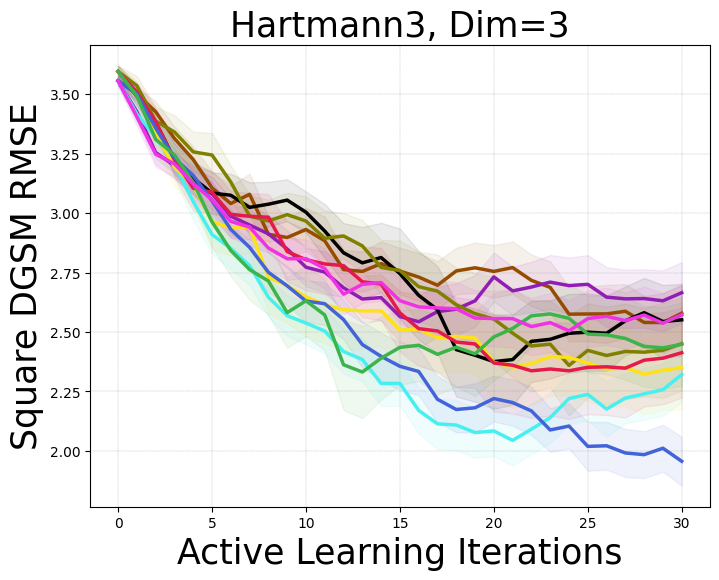
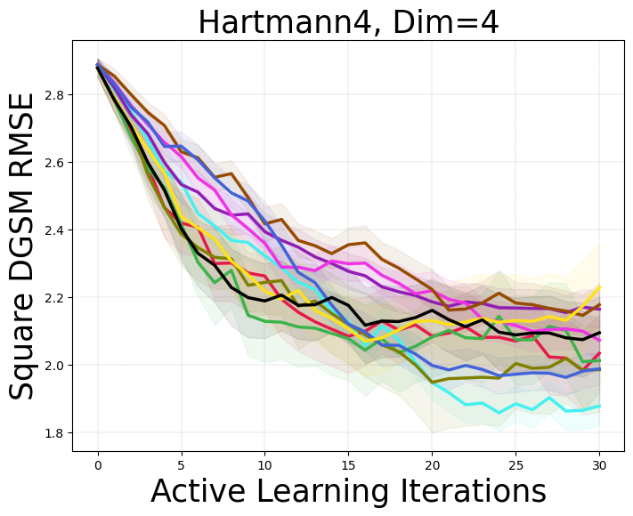
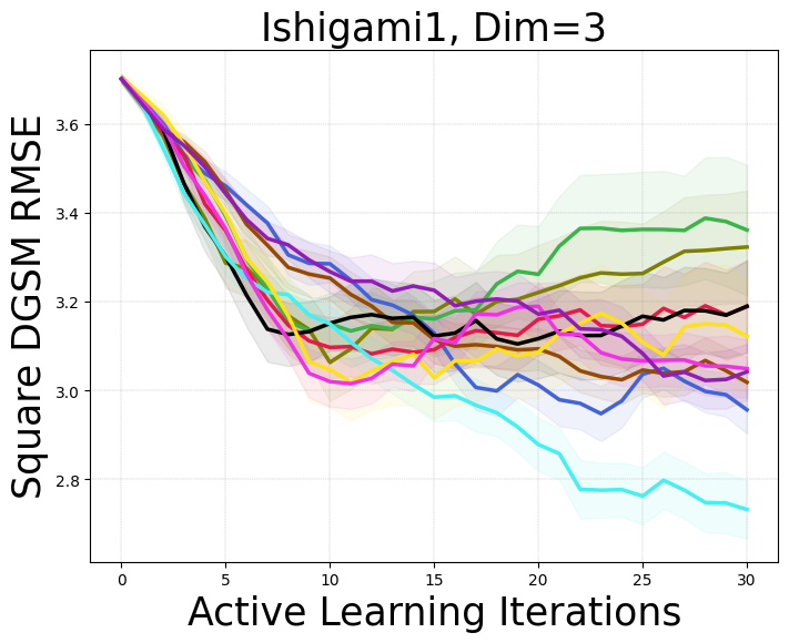
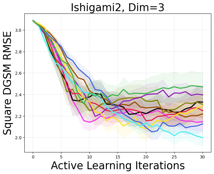
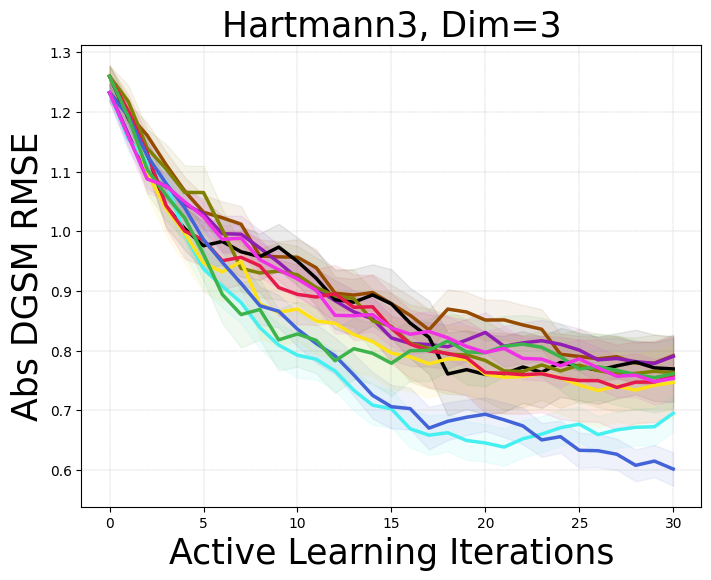
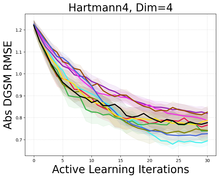
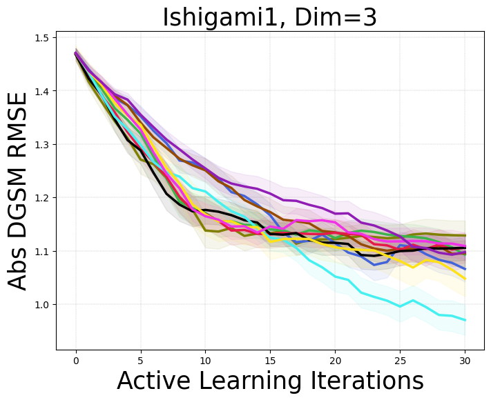
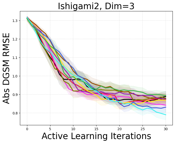
We conducted experiments on a family of functions that were designed specifically for evaluating sensitivity analysis measures [Kucherenko et al., 2009, Kucherenko and Iooss, 2014]: Ishigami1 ($d=3$), Ishigami2 ($d=3$), Gsobol6 ($d=6$), a-function ($d=6$), Gsobol10 ($d=10$), Gsobol15 ($d=15$) and Morris ($d=20$). Ground-truth DGSMs are available for these problems. Additionally, we tested the methods on other general-purpose synthetic functions where sensitivity might be challenging to estimate [Dixon, 1978]: Branin ($d=2$), Hartmann3 ($d=3$) and Hartmann4 ($d=4$). For these functions, we numerically estimated ground-truth DGSMs.

Real world problems.

We considered three real-world design problems. The Car Side Impact Weight problem simulates the impact of $d=7$ design variables on the weight of a car, to study the impact of weight on accident scenarios. Design variables are the thickness of pillars, the floor, cross members, etc. We also used the Vehicle Safety problem, which has two functions: the weight and the acceleration of the vehicle. Both are functions of $d=5$ design variables describing the thickness of frontal reinforcement materials. We study the two functions as independent problems. Ground truth DGSMs for these problems were estimated numerically.

Experimental setup.

We study settings with limited evaluation budgets. Quasirandom sequences are known to perform well given enough data [De Lozzo and Marrel, 2016, Chauhan et al., 2024]. Here, we focus on the restrictive case where we initialize our experiments using five random inputs and run 30 iterations of active learning. Our results are averaged over $50$ replicates from different initial points, and we report the mean and two standard errors over replicates. Our primary evaluation metric is root mean squared error (RMSE) of the DGSM estimate versus ground truth. All acquisition functions were implemented in the BoTorch framework [Balandat et al., 2020] (code available on Github ). All methods were implemented to be auto-differentiable and, therefore, are efficiently optimized with gradient optimization.

5.1 Results and Discussion

Figure 2: Synthetic and real-world experiments evaluated using the RMSE metric. The RMSE of the squared and absolute DGSMs is reported as the mean (and two standard errors shaded) over 50 runs of active learning. Active learning methods that target the derivatives consistently outperformed quasirandom sequences and active learning targeting $f$.

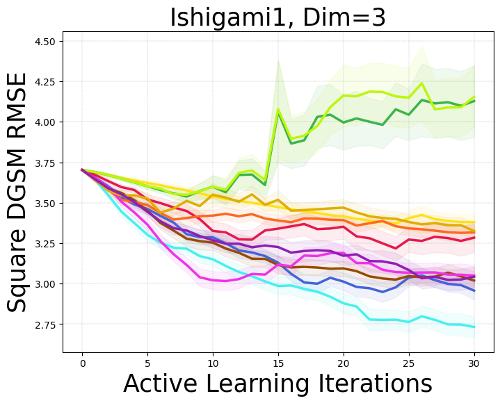
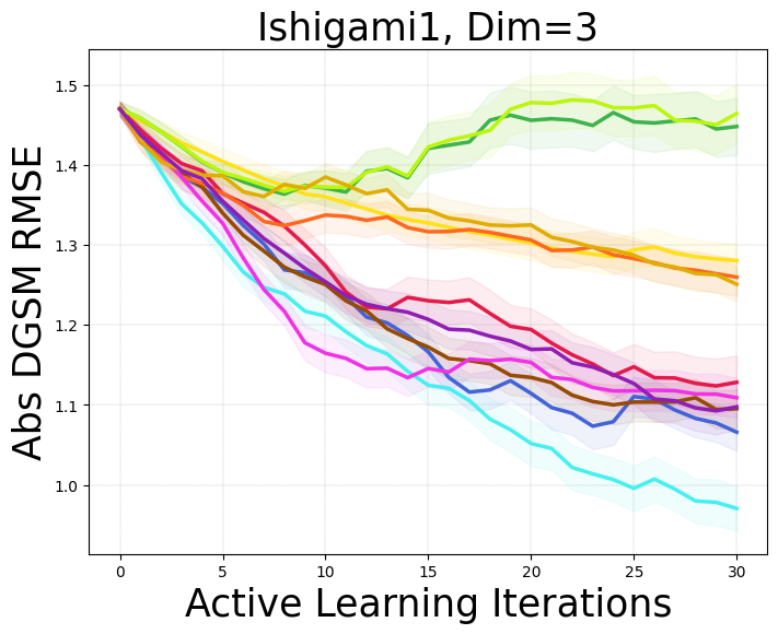
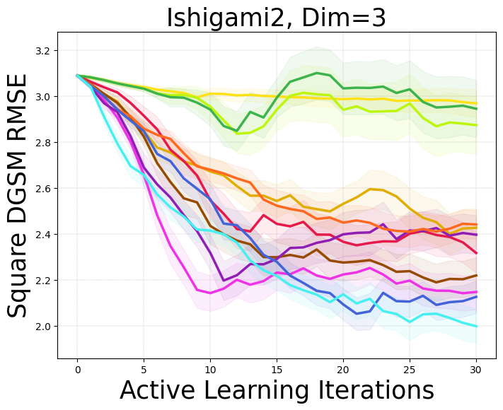
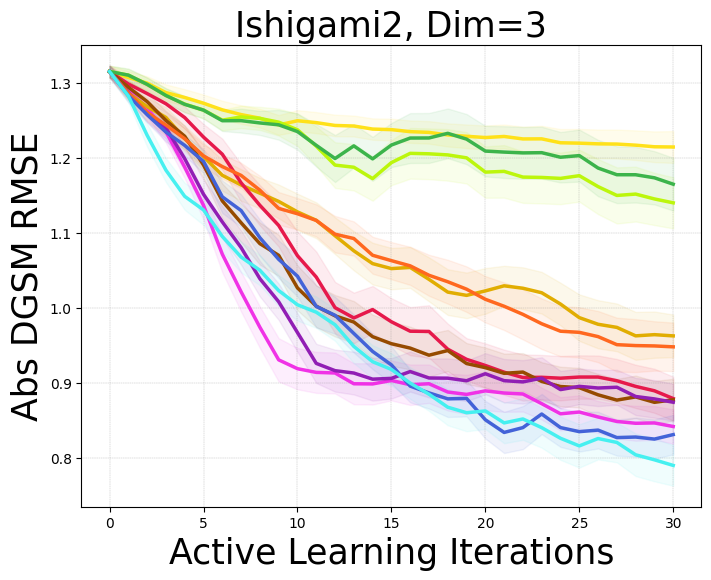
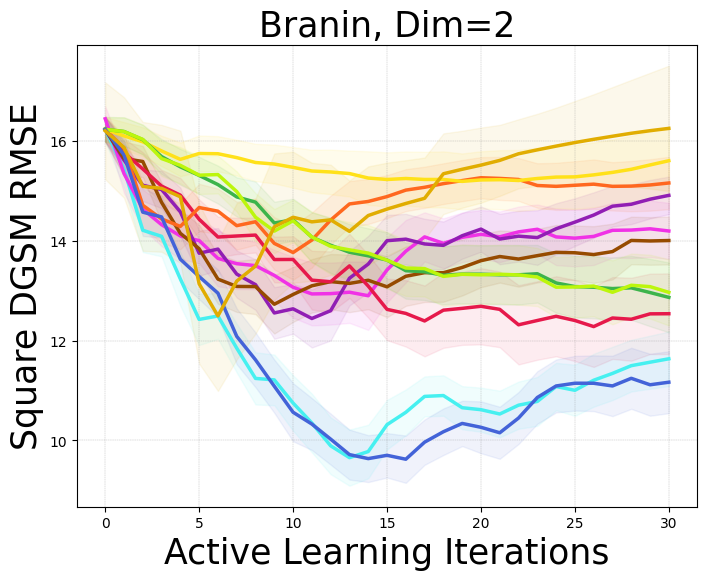
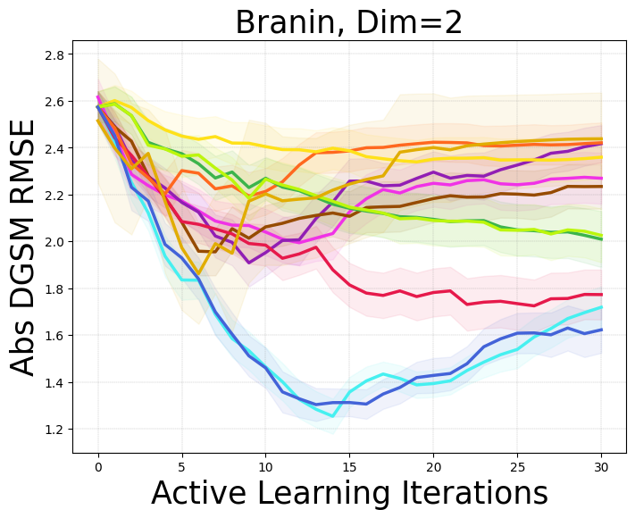
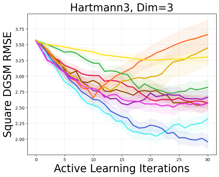
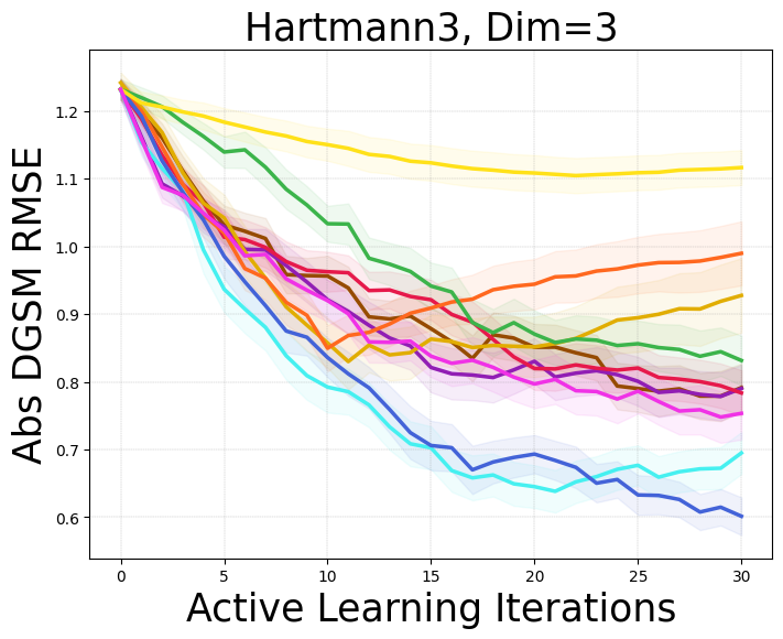
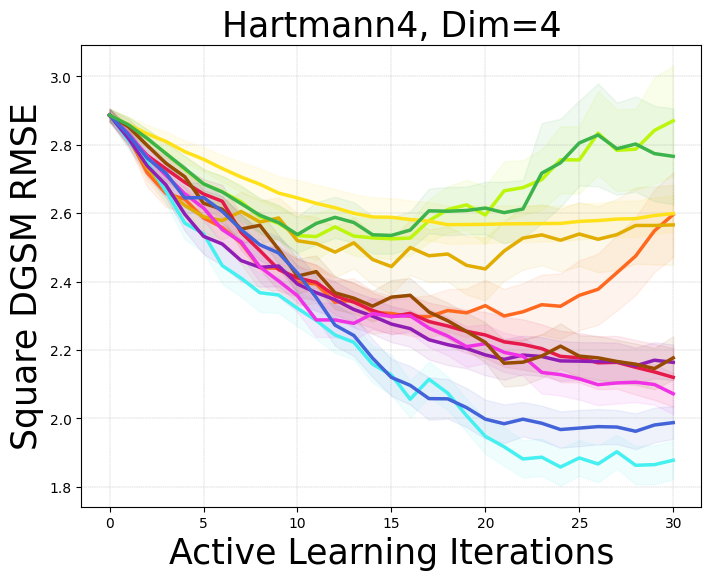
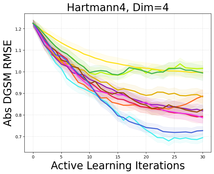
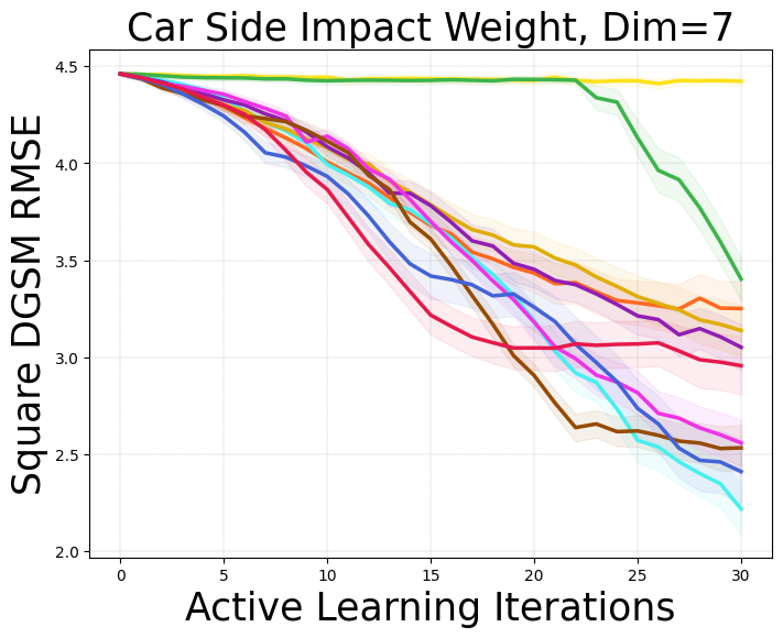
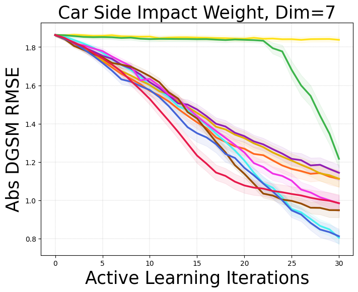
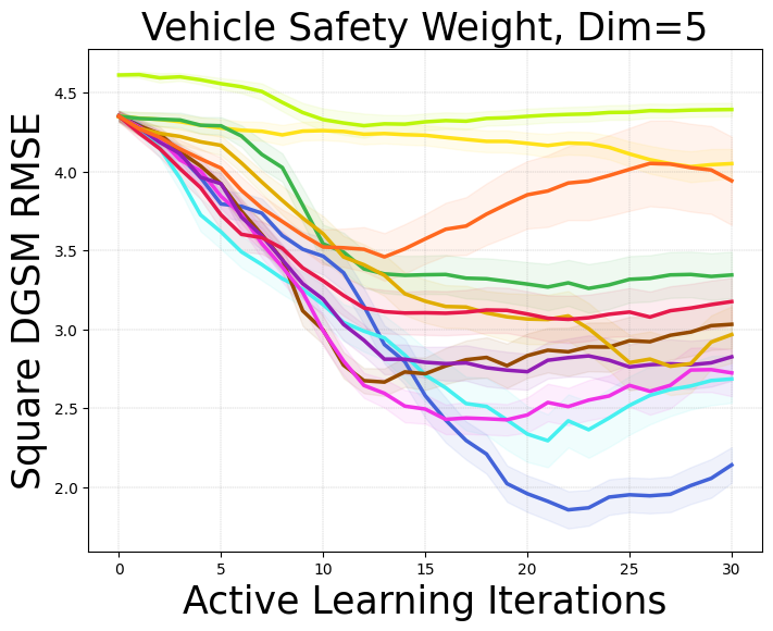
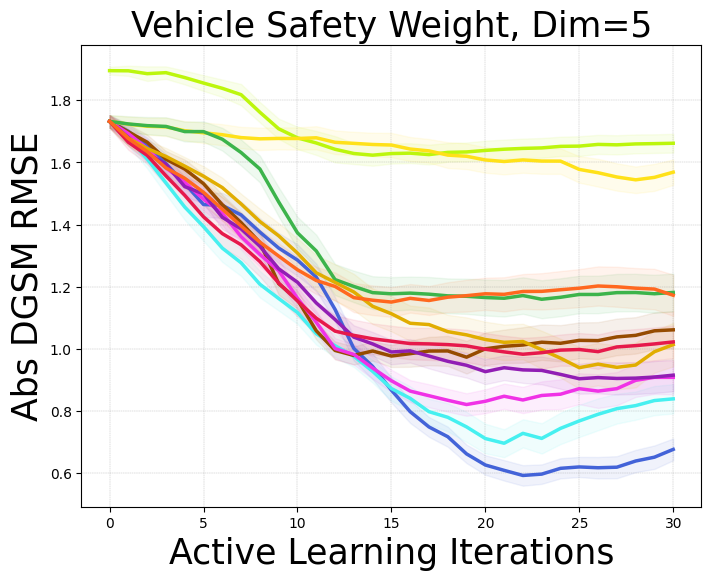
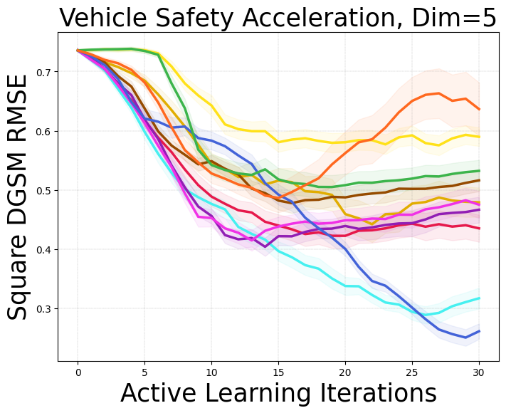
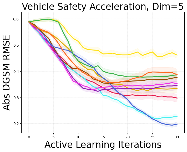
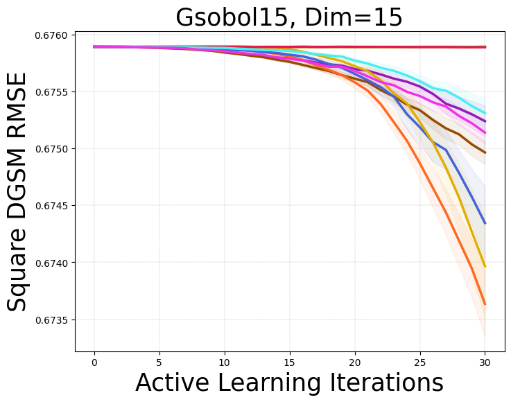
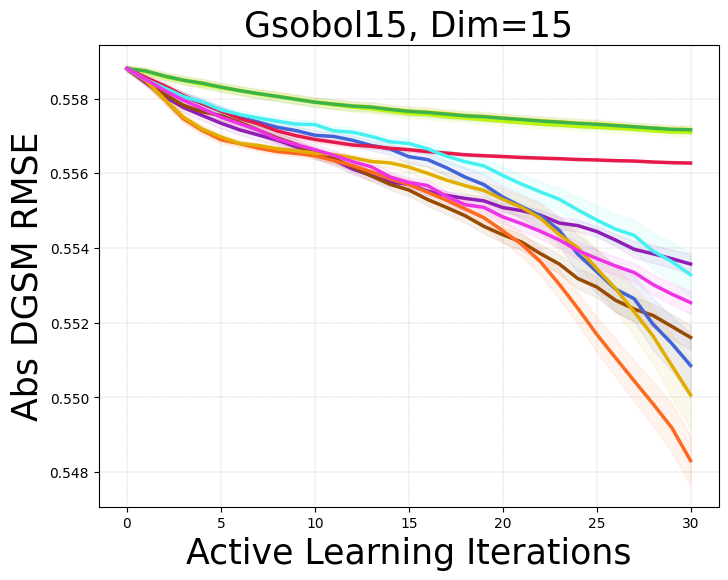
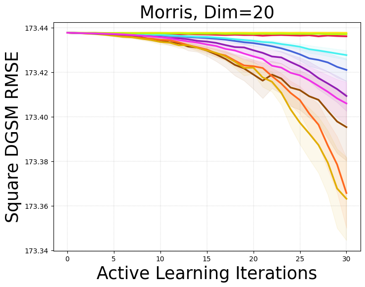
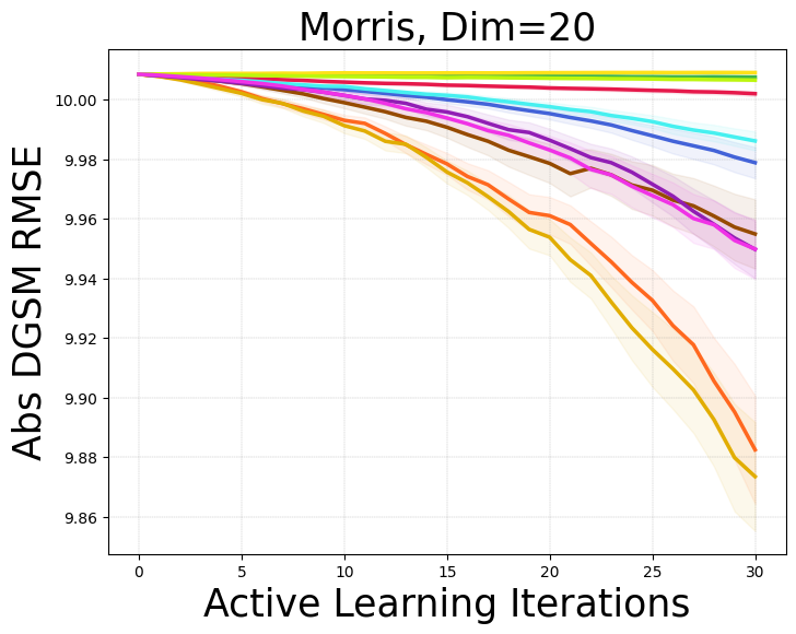
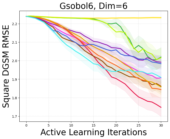
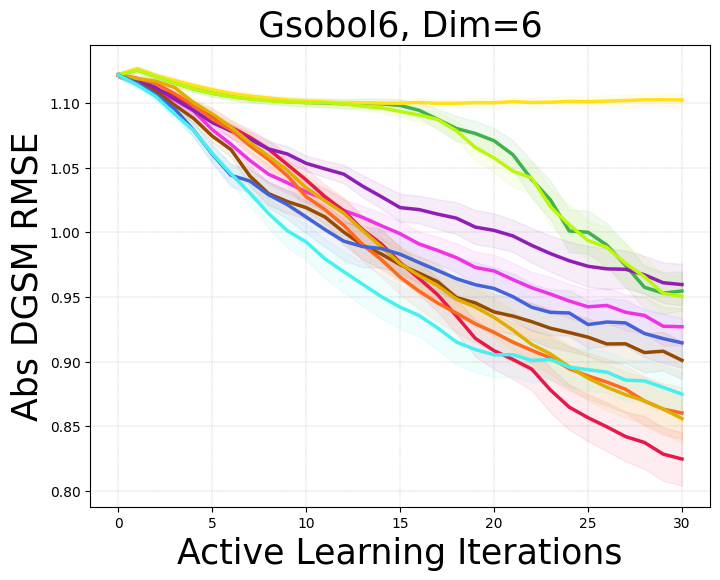
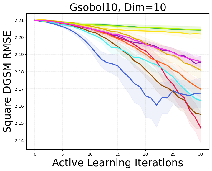
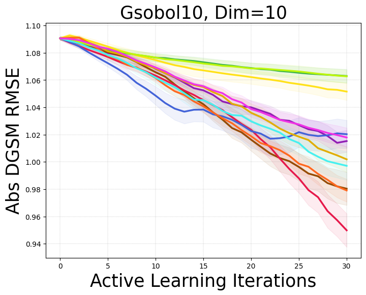
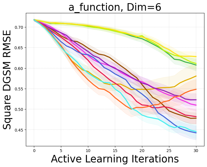
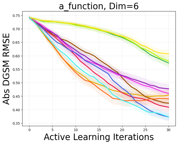
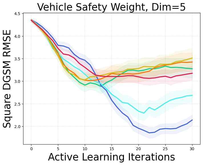
RMSE results for seven synthetic functions and three real-world problems (Figure 2, for both absolute and square DGSMs, show the benefits of our approach. Across this wide set of problems, the active learning approaches targeting quantities of the derivatives developed here consistently outperformed quasirandom sequences (qr) and active learning methods that target learning about $f$ globally (fvar and fig). The acquisition functions based on the information gain of the derivative (dig) and squared derivative (dsqig) performed best in the majority of experiments.

In the high-dimensional problems (GSobol15 and Morris), we see a substantial degradation of performance for the baseline methods (qr, fvar, and fig), with little reduction of RMSE across iterations. Our proposed active learning acquisition functions targeting the derivatives, on the other hand, continued to perform well in high dimensions. It is interesting to note that on these problems the derivative max variance acquisition functions, dabv, and dsqv, outperformed the derivative information gain acquisition functions. This is due to the myopic nature of the one-step look-ahead used for information gain. The most information gain about the derivative comes from adjacent points (Figure 1). In high dimensions, one-step look-ahead focuses on areas near existing observations, and is not exploratory enough to capture the whole function. Max variance is naturally more exploratory and thus performs better in high-dimensional settings. However, the derivative information gain acquisitions still outperform the baselines in high-dimensional settings.

5.2 Ablations and Additional Results

Ranking metrics.

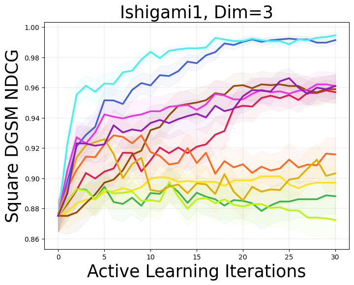
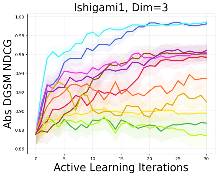
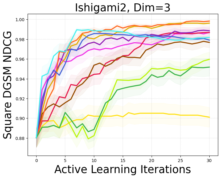
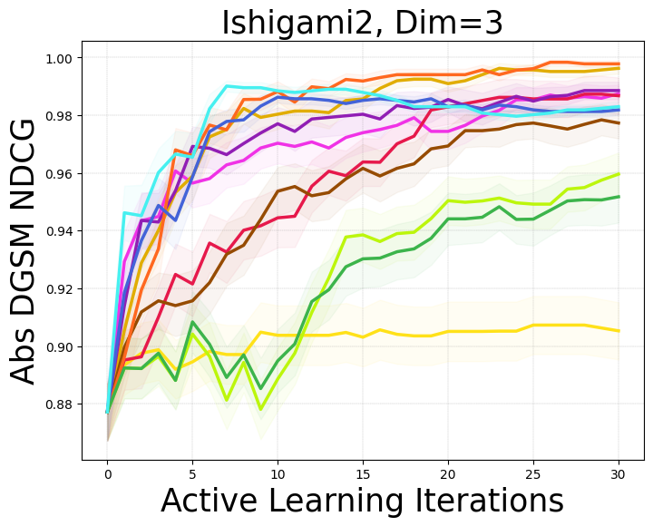
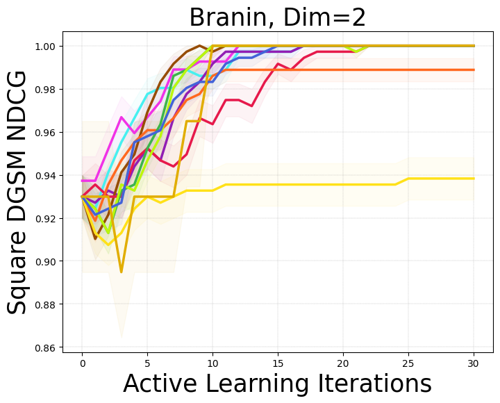
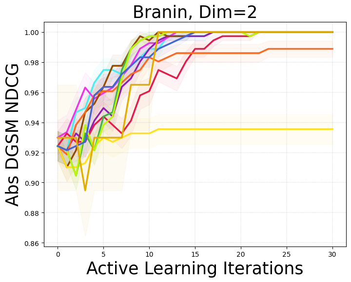
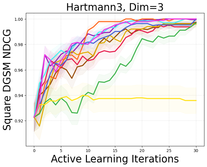
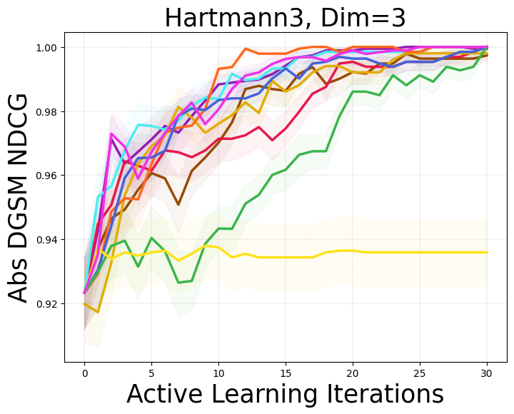
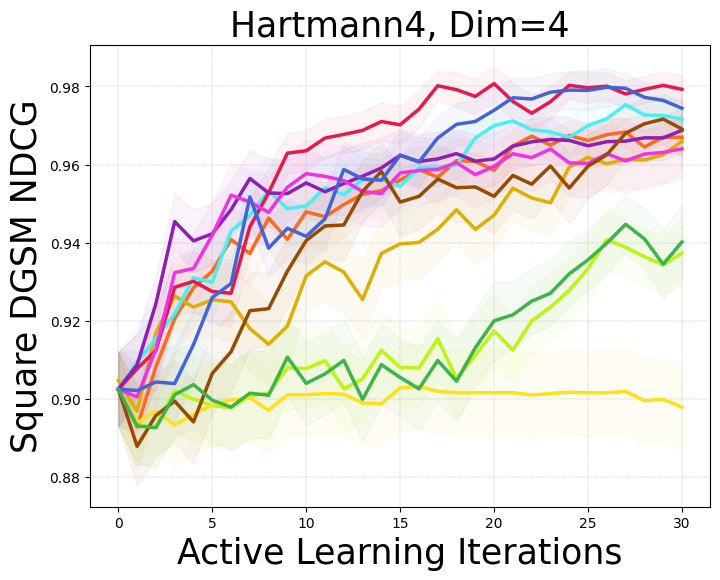
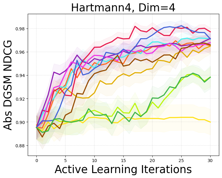
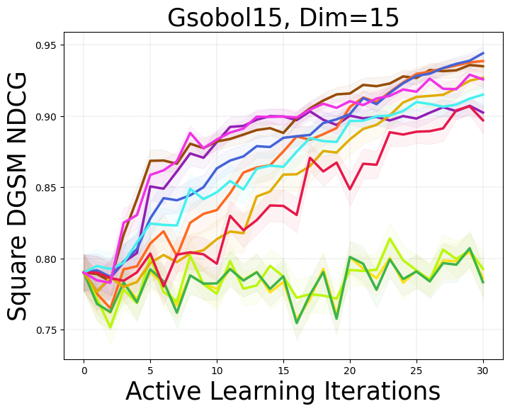
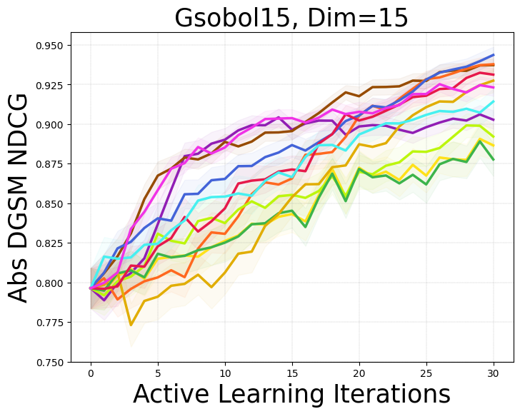
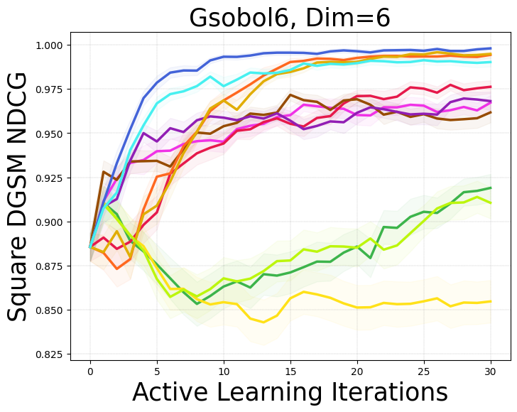
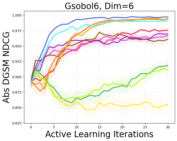
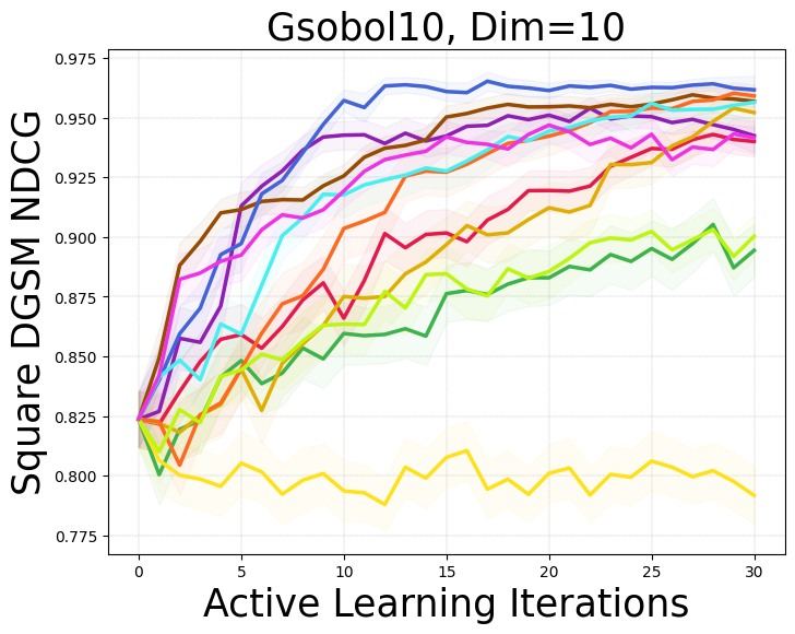
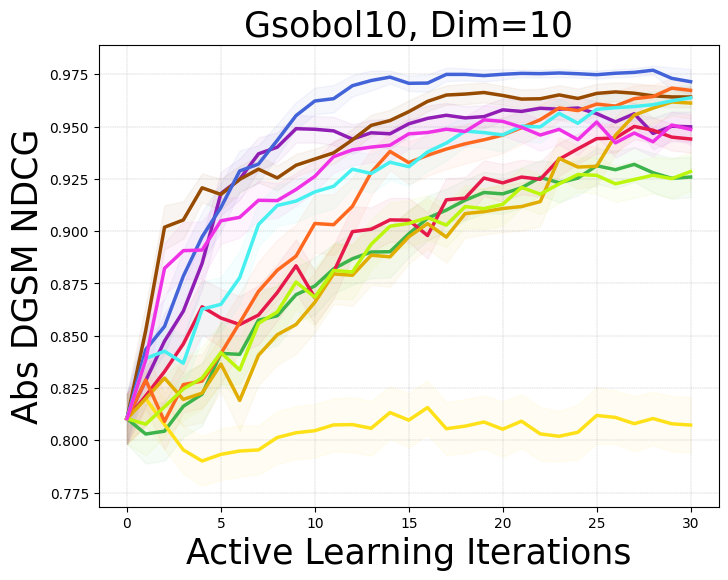
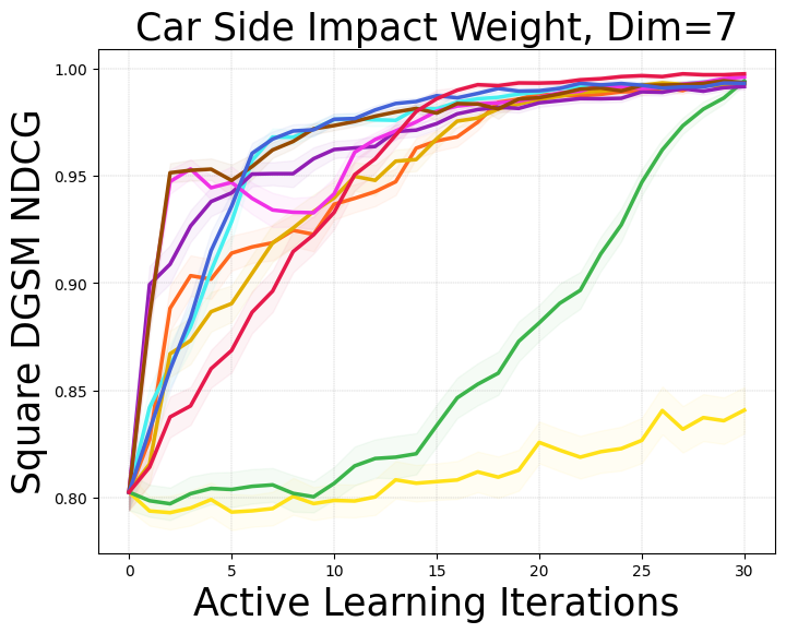
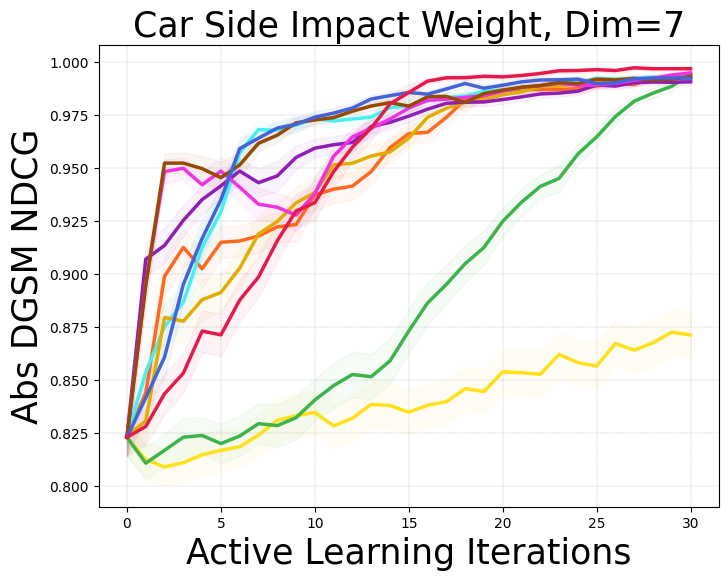
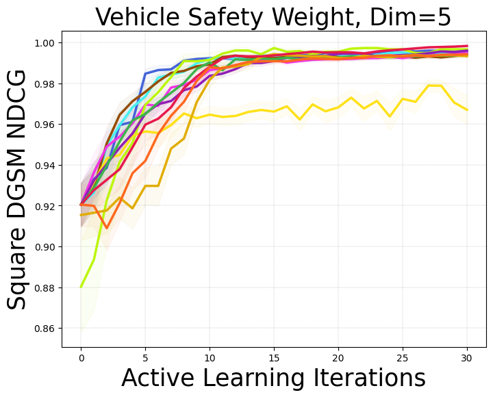
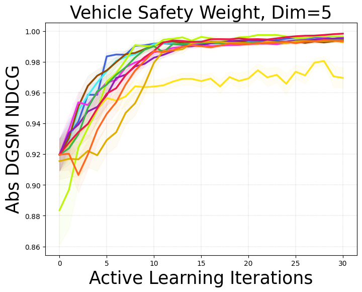
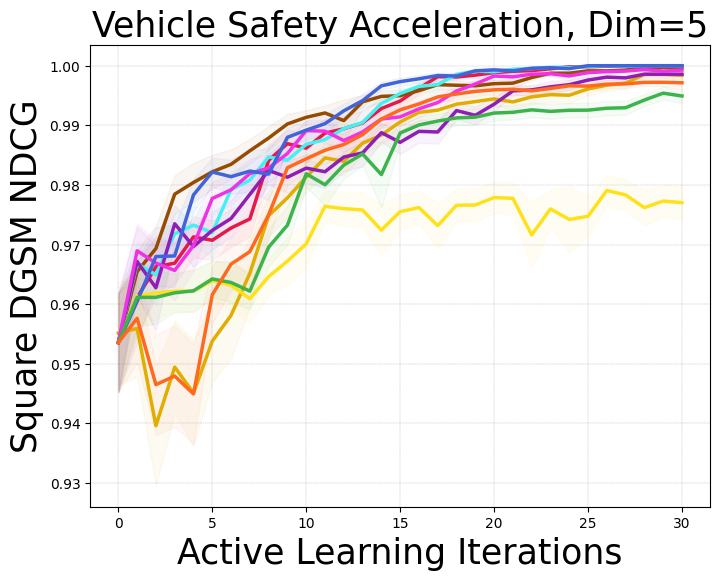
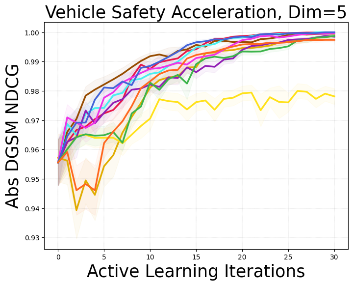
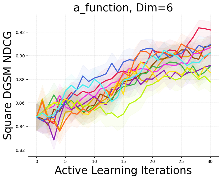
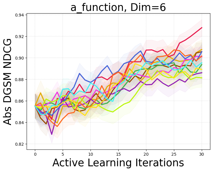
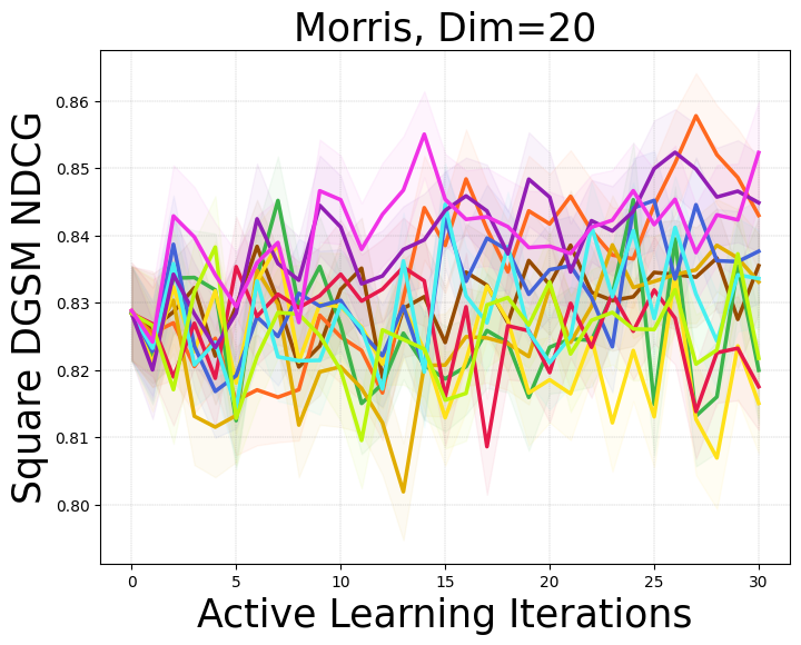
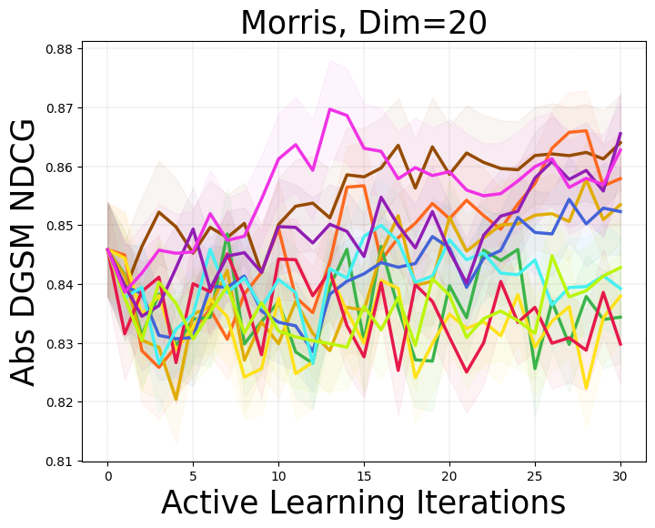
In settings where DGSMs are used to determine the relative importance of the variables, we are interested in the ability of the method to correctly rank the variables. We replaced RMSE as the evaluation metric with normalized discounted cumulative gain (NDCG) [Järvelin and Kekäläinen, 2002], a commonly used metric of ranking quality. NDCG accounts for the position of each dimension, giving higher importance to dimensions at the top of the list, and is normalized to a scale from 0 to 1, where 1 represents perfect recapitulation of the order. As with RMSE, dig and dsqig generally perform best on this task (Figure 5 in the Appendix).

Global variance reduction and information gain.

In the Appendix, we derive acquisition functions that evaluate the impact of observing $\mathbf{x}_{*}$ on the posterior globally, and integrate over that global effect. We show that, for learning DGSMs, the global acquisitions do not substantially improve over the local versions described in Section 4, while creating a large computational burden.

6 Conclusions

In this work, we developed a collection of active learning methods that directly target DGSMs. These strategies substantially enhanced the sample efficiency of DGSM estimation when compared to quasirandom search and even compared to active learning strategies targeting $f$. Information gain about the derivative and the squared derivative were generally the best approaches.

Our work paves the way for additional work on active learning for DGSMs in several directions. Although both variance reduction and information gain approaches perform well in high dimensions, information gain approaches might benefit from increased exploration by using a two-step or batch look-ahead to select pairs of points in acquisition function optimization. Our acquisition functions also all take the form of a sum over dimensions. Computing entropy of multivariate posteriors for the gradient is another possible avenue. Active learning for DGSMs could also be developed for non-Gaussian models. Finally, DGSMs have been linked via several lower/upper bound inequalities to ANOVA-based sensitivity indices [Kucherenko and Iooss, 2014]. Understanding the impact of active learning for DGSMs on ANOVA-based sensitivity indices is another useful direction for future work.

Active Learning for Derivative-Based Global Sensitivity Analysis with Gaussian Processes (Supplementary Material)

Appendix A Additional Discussion of Related Work

Here we give further discussion of lines of work that incorporate derivatives into active learning, albeit not for the purpose of GSA.

Goal-Oriented Sequential Design. Salem et al. [2019] proposed an optimization approach where at each step the dimensionality is reduced by identifying unimportant features. Unimportant variables are fixed while simultaneously optimizing the important ones with expected improvement. These variables are identified through their lengthscales. As part of theoretical analysis, the paper proves an asymptotic relationship between lengthscale and the square DGSM: as lengthscale goes to infinity, DGSM for that parameter goes to zero. This work does not propose an active learning approach for DGSMs but rather uses DGSMs as a metric to asses the quality of the dimensionality reduction approach. Spagnol et al. [2019] used sensitivity analysis to eliminate variables during optimization. The sensitivity analysis is goal-oriented rather than global, by applying the Hilbert–Schmidt independence criterion to portions of the function below a particular output quantile. Sensitivity measures are part of the algorithm and are assumed to be accurate, the paper does not study learning them.

Active learning in the presence of non-stationarity. Erickson et al. [2018] developed a method for active learning of a non-stationary function that specifically targets areas of high gradient, although without trying to estimate the gradient globally. Variance reduction of the function serves as the acquisition, but weighted by the estimated derivative and its variance. The method thus focuses on minimizing the variance at points with large derivatives, but does not target learning the derivative itself. Marmin et al. [2018] proposed an active learning approach for non-stationary functions using warping. The acquisition strategy uses both variance reduction and derivatives, following a similar idea as Erickson et al. [2018] that areas of high gradient will be helpful for learning the function.

Active Subspaces Learning. Wycoff et al. [2021] proposed a set of three methods (Trace, Var1, and Var2) for active subspace identification. While the goal is different from our proposed methods, the acquisition functions developed in the paper do aim to learn a quantity of the derivatives, as in our work. Specifically, the acquisitions attempt to learn the expectation of the outer product of the gradient. The elements of the diagonal of the outer product of the gradient are the squared DGSMs, so learning the outer product will learn a function of the squared DGSMs, albeit without targeting them specifically.

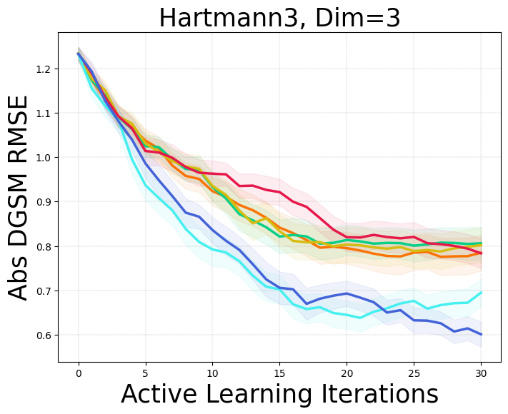
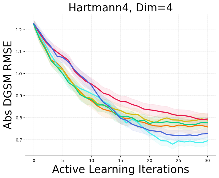
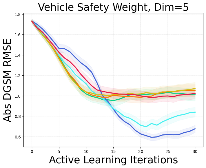
Because these methods target learning a function of the gradient, we compared against them on three representative problems. We used the reference implementation of the methods, from the R package activegp. The results are shown in Fig. 3. For clarity and due to the large number of methods, this figure includes only qr and dig alongside Trace, Var1, and Var2; performance relative to other methods can be seen by comparing the results to Fig. 2. The figure shows that active subspace learning methods do not perform as well as derivative information gain. While they do target a related quantity, learning the active subspace is not the most effective approach to learning the squared DGSM.

Figure 3: An empirical evaluation of active subspace methods on the task of learning the square and absolute DGSM, with derivative information gain, derivative square information gain, and quasirandom as points of comparison.

Appendix B Computational Complexity

All of our acquisition functions have closed-form expressions. Computing the GP posterior is $\mathcal{O}(t^{3}+t^{2}d)$, with $t$ the number of data and $d$ the dimensionality of the function. Here the $t^{3}$ comes from inverting $k_{X}$, and the $t^{2}d$ comes from multiplying it with the gradient of $k_{x*,X}$. Given that, the remaining computation will all scale linearly with $d$, since it is just applying various formulae to the posteriors for each dimension.

Appendix C Global Look-ahead Acquisition Functions

Our look-ahead acquisition functions were all local, in that they evaluated the impact of an observation at $\mathbf{x}_{*}$ only on the posterior at $\mathbf{x}_{*}$. In this section, we consider the global look-ahead acquisitions where we evaluate the impact on the posterior across the entire input space. These acquisition functions are expressed as integral over the previously proposed local acquisition functions. Their complexity is $\mathcal{O}(t^{3}+t^{2}dM)$, with $M$ defined as the granularity of the integration. We provide the results and discussion in Appendix D.

C.1 Derivative Look-Ahead Distribution at Different Input Location

We wish to predict the impact that observing $f$ at a candidate location $\mathbf{x}_{*}$ will have on the model’s derivatives at a different location $\mathbf{x}_{+}$. This will allow us to select a point $\mathbf{x}_{*}$ that most improves the model of the derivatives in the overall search space, in expectation. Under a GP, this look-ahead distribution is tractable. Conditioned on the observations $\mathcal{D}$, $f(\mathbf{x}_{*})$ and $\frac{\partial f(\mathbf{x}_{+})}{\partial x_{i}}$ have a bivariate normal joint distribution for each input dimension $i$. The formula for bivariate normal conditioning once again provides the look-ahead distribution:

$$\frac{\partial f(\mathbf{x}_{+})}{\partial x_{i}}\biggm{\lvert}f(\mathbf{x}_{*})=y_{*},\mathcal{D}\sim\mathcal{N}\left(\mu_{+|*,i}^{\prime\ell},(\sigma_{+|*,i}^{\prime\ell})^{2}\right),$$

where the look-ahead mean and variance are respectively

$$\mu_{+|*,i}^{\prime\ell}=\mu^{\prime}_{+,i}+\frac{\tilde{\sigma}_{+*,i}}{\sigma_{*}^{2}}(y_{*}-\mu_{*}),~{}~{}~{}~{}~{}(\sigma_{+|*,i}^{\prime\ell})^{2}=(\sigma^{\prime}_{+,i})^{2}-\left(\frac{\tilde{\sigma}_{+*,i}}{\sigma_{*}}\right)^{2}$$ (5)

with $\tilde{\sigma}_{+*,i}=\textrm{Cov}[f(\mathbf{x}_{*}),\frac{\partial f(\mathbf{x}_{+})}{\partial x_{i}}|\mathcal{D}]$ the posterior covariance between $f$ at $\mathbf{x}_{*}$ and the derivative at $\mathbf{x}_{+}$, and $(\sigma^{\prime}_{+,i})^{2}=\sigma^{\prime}_{i}(\mathbf{x}_{+})^{2}=\left[\Sigma^{\prime}(\mathbf{x}_{+})\right]_{ii}$ the posterior variance of the derivative. We use a similar notation short-hand $\sigma_{+|*,i}^{\prime\ell}=\sigma_{i}^{\prime\ell^{*}}(\mathbf{x}_{+})$ and $\mu_{+|*,i}^{\prime\ell}=\mu_{i}^{\prime\ell^{*}}(\mathbf{x}_{+})$ as the look-ahead posterior mean and variance at the input $\mathbf{x}_{+}$ if $(\mathbf{x}_{*},y_{*})$ were added to the data.

C.2 Global Look-Ahead Gradient Acquisition Functions

We first develop the global version of the look-ahead acquisition functions targeting the uncertainty and information gain about the derivative of the GP.

Global variance reduction.

We compute the global expected reduction in variance produced by an observation at $\mathbf{x}_{*}$ as follows:

$$\alpha_{\textrm{{gd}{v}\textsubscript{r}{}}}(\mathbf{x}_{*})=\frac{1}{|\mathcal{X}|}\int_{\mathcal{X}}\sum_{i=1}^{d}\sigma_{i}^{\prime}(\mathbf{x})^{2}-\mathbb{E}_{y_{*}}[\sigma_{i}^{\prime\ell^{*}}(\mathbf{x})^{2}]d\mathbf{x}=\frac{1}{|\mathcal{X}|}\int_{\mathcal{X}}\sum_{i=1}^{d}\sigma_{i}^{\prime}(\mathbf{x})^{2}-\hat{\sigma}_{i}^{\prime\ell^{*}}(\mathbf{x})^{2}d\mathbf{x}.$$

Global information gain.

As before, the information gain is:

$$\alpha_{\textrm{{gdig}{}}}(\mathbf{x}_{*}) =\frac{1}{|\mathcal{X}|}\int_{\mathcal{X}}\sum_{i=1}^{d}H^{\prime}_{i}(\mathbf{x})-\mathbb{E}_{y_{*}}\left[H^{\prime}_{i}(\mathbf{x}|f(\mathbf{x}_{*})=y_{*}\right)]d\mathbf{x}$$

$$=\frac{1}{|\mathcal{X}|}\int_{\mathcal{X}}\frac{1}{2}\sum_{i=1}^{d}\log(2\pi\sigma_{i}^{\prime}(\mathbf{x})^{2})-\log(2\pi\sigma_{i}^{\prime\ell^{*}}(\mathbf{x})^{2})d\mathbf{x}.$$

C.3 Global absolute gradient acquisition functions.

Next we develop acquisition functions that seek to learn the absolute value of the derivative.

Global variance reduction.

As before,

$$\alpha_{\textrm{{gda}{b}{v}\textsubscript{r}{}}}(\mathbf{x}_{*})=\frac{1}{|\mathcal{X}|}\int_{\mathcal{X}}\sum_{i=1}^{d}\sigma_{i_{Ab}}^{\prime}(\mathbf{x})^{2}-\mathbb{E}_{y_{*}}[\sigma_{i_{Ab}}^{\prime\ell^{*}}(\mathbf{x})^{2}]d\mathbf{x}\approx\frac{1}{|\mathcal{X}|}\int_{\mathcal{X}}\sum_{i=1}^{d}\sigma_{i_{Ab}}^{\prime}(\mathbf{x})^{2}-\hat{\sigma}_{i_{Ab}}^{\prime\ell^{*}}(\mathbf{x})^{2}d\mathbf{x},$$

which we approximate using the plug-in estimator $\hat{\sigma}_{i_{Ab}}^{\prime\ell^{*}}(\mathbf{x})^{2}$.

C.4 Global Squared Gradient Acquisition Functions

The final set of acquisition functions are developed based on the uncertainty and information gain about the squared derivative of the GP.

Global Variance Reduction

We again approximate the variance reduction with a plug-in estimator to get an estimate for the look-ahead variance of the squared derivative:

$$\hat{\sigma}_{i_{sq}}^{\prime\ell^{*}}(\mathbf{x})^{2}=4\sigma_{i}^{\prime\ell^{*}}(\mathbf{x})^{2}\mu_{i}^{\prime}(\mathbf{x})^{2}+2\sigma_{i}^{\prime\ell^{*}}(\mathbf{x})^{4},$$

which is independent of $y_{*}$. Variance reduction can then be computed as

$$\alpha_{\textrm{{gds}{q}{v}\textsubscript{r}{}}}(\mathbf{x}_{*}) =\frac{1}{|\mathcal{X}|}\int_{\mathcal{X}}\sum_{i=1}^{d}\sigma_{i_{sq}}^{\prime}(\mathbf{x})^{2}-\mathbb{E}_{y_{*}}[\sigma_{i_{sq}}^{\prime\ell^{*}}(\mathbf{x})^{2}]d\mathbf{x}$$

$$\approx\frac{1}{|\mathcal{X}|}\int_{\mathcal{X}}\sum_{i=1}^{d}\sigma_{i_{sq}}^{\prime}(\mathbf{x})^{2}-\hat{\sigma}_{i_{sq}}^{\prime\ell^{*}}(\mathbf{x})^{2}d\mathbf{x}.$$

Global information gain

We use the same plug-in estimator as before to get $\hat{r}^{\ell^{*}}_{i}(\mathbf{x})=\frac{\mu_{i}^{\prime}(\mathbf{x})}{\sigma_{i}^{\prime\ell^{*}}(\mathbf{x})}$. The approximated look-ahead entropy is then

$$\hat{H}^{sq,*}_{i}(\mathbf{x})=2\log(\sigma_{i}^{\prime\ell^{*}}(\mathbf{x}))-\prescript{}{2}{F}_{2}\left(1,1,\frac{3}{2},2,-\frac{\hat{r}_{i}^{\ell^{*}}(\mathbf{x})^{2}}{2}\right)\hat{r}_{i}^{\ell^{*}}(\mathbf{x})^{2},$$

and

$$\alpha_{\textrm{{gds}{q}{ig}{}}}(\mathbf{x}_{*})\approx\frac{1}{|\mathcal{X}|}\int_{\mathcal{X}}\sum_{i=1}^{d}H^{sq}_{i}(\mathbf{x})-\hat{H}^{sq}_{i}(\mathbf{x})d\mathbf{x}.$$

For all of these global acquisition functions, the integral over the input space is estimated with QMC sampling, meaning the impact of the observation at $\mathbf{x}_{*}$ is evaluated on a global reference set of size $M$, over which the acquisition function is averaged.

Appendix D Additional Results and Discussion

In this section we provide additional experimental results.

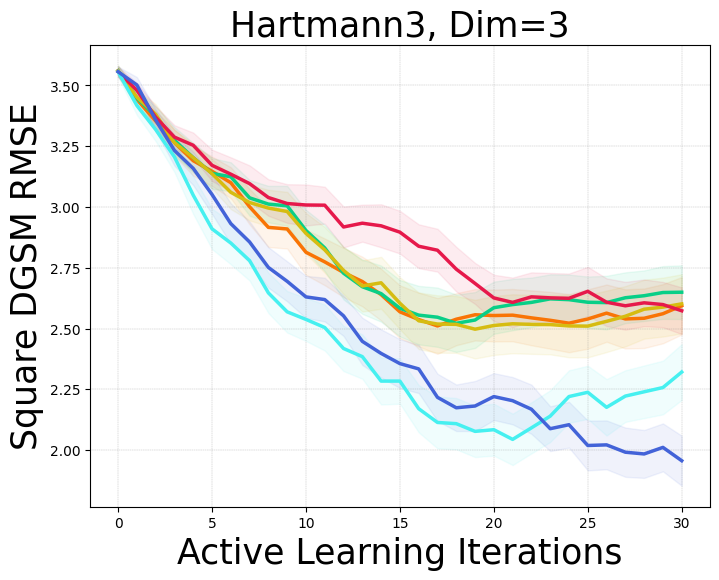
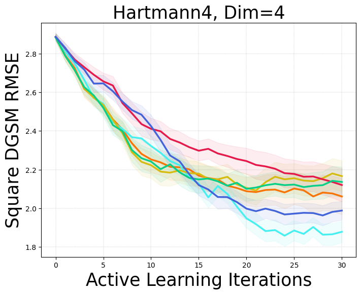
Additional Results for RMSE In Figure 4, we provide additional results on synthetic functions evaluated with RMSE.

Results and Discussion for Ranking metrics In Figure 5, we show the performance evaluated with NDCG (discussion provided in the main paper). Figure 6 shows the results of the ranking metric NDCG for two synthetic functions a-function and Morris. We notice an instability in their ranking results. These two particular problems have several dimensions with the same ranking and/or very close DGSMs values. Due to these factors, the ranking of the variables changes frequently over iterations leading to the instability in the curves. However, by analyzing the RMSE results, we can see that the active learning algorithms are still capable of approximating the true DGSMs values.

Results and Discussion for Global Look-ahead Acquisition functions In this study, we compare the local look-ahead acquisition functions proposed in the main paper to the global look-ahead acquisition functions developed in Appendix C. For the local acquisition functions we use their acronyms provided in Section 4. For the global acquisition functions we use their acronyms provided in Appendix C: the global variance reduction of the absolute and squared derivatives are gdabv_r and gdsqv_r; and information gain of the raw and squared derivatives are gdig and gdsqig.

As discussed above, the complexity of the global acquisition function depends on the granularity of the numerical integration. Given that the granularity of the integration $M$ needs to be high for numerical accuracy, the computational time and memory requirement becomes prohibitive, especially in high dimensions. Figure 7 shows that despite the extra computational cost, the global acquisition functions have comparable performance for variance reduction and lower performance for information gain than their local versions. Given the high computational cost incurred by the integration, we believe the local acquisition functions are more practical.

Figure 4: Additional synthetic experiments evaluated using RMSE. The RMSE of the square DGSMs and absolute DGSMs is reported with the mean and two standard errors of 50 repeats.

Figure 5: Synthetic and real-world experiments evaluated using NDCG. The NDCG of the square DGSMs and absolute DGSMs is reported with the mean and two standard errors of 50 repeats.

Figure 6: Synthetic experiments with multiple variables holding the same ranking evaluated using NDCG. The NDCG of the square DGSMs and absolute DGSMs is reported with the mean and two standard errors of 50 repeats.

Figure 7: Experiments comparing the global (integrated) information gain and variance reduction acquisition function to their local (non-integrated) version. The RMSE of the square DGSMs and absolute DGSMs is reported with the mean and two standard errors of 50 repeats.

References

- Balandat et al. [2020] M. Balandat, B. Karrer, D. R. Jiang, S. Daulton, B. Letham, A. G. Wilson, and E. Bakshy. BoTorch: a framework for efficient Monte-Carlo Bayesian optimization. In Advances in Neural Information Processing Systems 33, NeurIPS, 2020.
- Chauhan et al. [2024] M. S. Chauhan, M. Ojeda-Tuz, R. A. Catarelli, K. R. Gurley, D. Tsapetis, and M. D. Shields. On active learning for Gaussian process-based global sensitivity analysis. Reliability Engineering & System Safety, page 109945, 2024.
- Ciriello et al. [2019] V. Ciriello, I. Lauriola, and D. M. Tartakovsky. Distribution-based global sensitivity analysis in hydrology. Water Resources Research, 55(11):8708–8720, 2019.
- Cover [1999] T. M. Cover. Elements of Information Theory. John Wiley & Sons, 1999.
- De Lozzo and Marrel [2016] M. De Lozzo and A. Marrel. Estimation of the derivative-based global sensitivity measures using a Gaussian process metamodel. SIAM/ASA Journal on Uncertainty Quantification, 4(1):708–738, 2016.
- Dick et al. [2013] J. Dick, F. Y. Kuo, and I. H. Sloan. High-dimensional integration: the quasi-Monte Carlo way. Acta Numerica, 22:133–288, 2013.
- Dixon [1978] L. C. W. Dixon. The global optimization problem: an introduction. Towards Global Optimiation 2, pages 1–15, 1978.
- Erickson et al. [2018] C. B. Erickson, B. E. Ankenman, M. Plumlee, and S. M. Sanchez. Gradient based criteria for sequential design. In 2018 Winter Simulation Conference (WSC), pages 467–478. IEEE, 2018.
- Forrester et al. [2008] A. I. J. Forrester, A. Sóbester, and A. J. Keane. Engineering Design via Surrogate Modelling: a Practical Guide. Wiley, 2008.
- Gustafson et al. [1996] P. Gustafson, C. Srinivasan, and L. Wasserman. Local sensitivity analysis. Bayesian Statistics, 5:197–210, 1996.
- Houlsby et al. [2011] N. Houlsby, F. Huszár, Z. Ghahramani, and M. Lengyel. Bayesian active learning for classification and preference learning. arXiv preprint arXiv:1112.5745, 2011.
- Iooss and Saltelli [2017] B. Iooss and A. Saltelli. Introduction to sensitivity analysis. In Handbook of Uncertainty Quantification, pages 1103–1122. Springer, 2017.
- Järvelin and Kekäläinen [2002] K. Järvelin and J. Kekäläinen. Cumulated gain-based evaluation of IR techniques. ACM Transactions on Information Systems, 20(4):422–446, 2002.
- Kiparissides et al. [2009] A. Kiparissides, S. S. Kucherenko, A. Mantalaris, and E. N. Pistikopoulos. Global sensitivity analysis challenges in biological systems modeling. Industrial & Engineering Chemistry Research, 48(15):7168–7180, 2009.
- Krause et al. [2008] A. Krause, A. Singh, and C. Guestrin. Near-optimal sensor placements in Gaussian processes: Theory, efficient algorithms and empirical studies. Journal of Machine Learning Research, 9(2):235–284, 2008.
- Kucherenko and Iooss [2014] S. Kucherenko and B. Iooss. Derivative based global sensitivity measures. arXiv preprint arXiv:1412.2619, 2014.
- Kucherenko et al. [2009] S. Kucherenko, M. Rodriguez-Fernandez, C. Pantelides, and N. Shah. Monte Carlo evaluation of derivative-based global sensitivity measures. Reliability Engineering & System Safety, 94(7):1135–1148, 2009.
- Lam and Notz [2008] C. Q. Lam and W. I. Notz. Sequential adaptive designs in computer experiments for response surface model fit. Statistics and Applications, 6(1 & 2):207–233, 2008.
- Le Gratiet et al. [2014] L. Le Gratiet, M. Couplet, B. Iooss, and L. Pronzato. Planification d’expériences séquentielle pour l’analyse de sensibilité. 46èmes Journées de Statistique, Rennes (France), 60, 2014.
- Le Gratiet et al. [2017] L. Le Gratiet, S. Marelli, and B. Sudret. Metamodel-based sensitivity analysis: polynomial chaos expansions and Gaussian processes. In Handbook of Uncertainty Quantification, pages 1289–1325. Springer, 2017.
- Lyu et al. [2021] X. Lyu, M. Binois, and M. Ludkovski. Evaluating Gaussian process metamodels and sequential designs for noisy level set estimation. Statistics and Computing, 31(4):43, 2021.
- Marmin et al. [2018] S. Marmin, D. Ginsbourger, J. Baccou, and J. Liandrat. Warped Gaussian processes and derivative-based sequential designs for functions with heterogeneous variations. SIAM/ASA Journal on Uncertainty Quantification, 6(3):991–1018, 2018.
- McKay et al. [1979] M. D. McKay, R. J. Beckman, and W. J. Conover. A comparison of three methods for selecting values of output variables in the analysis of output from a computer code. Technometrics, 21(2):239–245, 1979.
- Moser [2020] S. M. Moser. Expected logarithm and negative integer moments of a noncentral -distributed random variable. Entropy, 22(9):1048, 2020.
- Owen [1998] A. B. Owen. Scrambling Sobol’ and Niederreiter-Xing points. Journal of Complexity, 14:466–489, 1998.
- Pfingsten [2006] T. Pfingsten. Bayesian active learning for sensitivity analysis. In European Conference on Machine Learning, ECML, pages 353–364, 2006.
- Prieur and Tarantola [2017] C. Prieur and S. Tarantola. Variance-based sensitivity analysis: Theory and estimation algorithms. Handbook of uncertainty quantification, pages 1217–1239, 2017.
- Qian et al. [2019] G. Qian, M. Massenzio, D. Brizard, and M. Ichchou. Sensitivity analysis of complex engineering systems: Approaches study and their application to vehicle restraint system crash simulation. Reliability Engineering & System Safety, 187:110–118, 2019.
- Rasmussen and Williams [2006] C. E. Rasmussen and C. K. I. Williams. Gaussian Processes for Machine Learning. MIT Press, 2006.
- Razavi and Gupta [2015] S. Razavi and H. V. Gupta. What do we mean by sensitivity analysis? The need for comprehensive characterization of “global" sensitivity in earth and environmental systems models. Water Resources Research, 51(5):3070–3092, 2015.
- Salem et al. [2019] M. B. Salem, F. Bachoc, O. Roustant, F. Gamboa, and L. Tomaso. Gaussian process-based dimension reduction for goal-oriented sequential design. SIAM/ASA Journal on uncertainty quantification, 7(4):1369–1397, 2019.
- Saltelli et al. [2008] A. Saltelli, M. Ratto, T. Andres, F. Campolongo, J. Cariboni, D. Gatelli, M. Saisana, and S. Tarantola. Global Sensitivity Analysis: the Primer. John Wiley & Sons, 2008.
- Schein and Ungar [2007] A. I. Schein and L. H. Ungar. Active learning for logistic regression: an evaluation. Machine Learning, 68:235–265, 2007.
- Sepúlveda et al. [2014] F. D. Sepúlveda, L. A. Cisternas, and E. D. Gálvez. The use of global sensitivity analysis for improving processes: applications to mineral processing. Computers & Chemical Engineering, 66:221–232, 2014.
- Shewry and Wynn [1987] M. C. Shewry and H. P. Wynn. Maximum entropy sampling. Journal of Applied Statistics, 14(2):165–170, 1987.
- Spagnol et al. [2019] A. Spagnol, R. L. Riche, and S. D. Veiga. Global sensitivity analysis for optimization with variable selection. SIAM/ASA Journal on uncertainty quantification, 7(2):417–443, 2019.
- Tsagris et al. [2014] M. Tsagris, C. Beneki, and H. Hassani. On the folded normal distribution. Mathematics, 2(1):12–28, 2014.
- Van Stein et al. [2022] B. Van Stein, E. Raponi, Z. Sadeghi, N. Bouman, R. C. Van Ham, and T. Bäck. A comparison of global sensitivity analysis methods for explainable AI with an application in genomic prediction. IEEE Access, 10:103364–103381, 2022.
- Wagener and Pianosi [2019] T. Wagener and F. Pianosi. What has global sensitivity analysis ever done for us? a systematic review to support scientific advancement and to inform policy-making in earth system modelling. Earth-Science Reviews, 194:1–18, 2019.
- Wainwright et al. [2014] H. M. Wainwright, S. Finsterle, Y. Jung, Q. Zhou, and J. T. Birkholzer. Making sense of global sensitivity analyses. Computers & Geosciences, 65:84–94, 2014.
- Wycoff et al. [2021] N. Wycoff, M. Binois, and S. M. Wild. Sequential learning of active subspaces. Journal of Computational and Graphical Statistics, 30(4):1224–1237, 2021.