Why scalar field is indispensable in Teleparallel Gravity theory?
Abstract
Teleparallel gravity theories were proposed as alternatives to the dark energy and modified theories of gravity. However, both the metric and symmetric teleparallel gravity theories have been found to have serious pathologies, such as coupling issues and Ostrogradski’s instability leading to ghost degrees of freedom. In this article we explore the fact that the theories are at-least free from the issue of ‘Branched Hamiltonian’ though, nonetheless, early inflation as well as a viable radiation era may only be driven by a scalar field.
1,3 Dept. of Physics, Jangipur College, Murshidabad, West Bengal, India - 742213,
1,2 Dept. of Physics, University of Kalyani, Nadia, West Bengal, India - 741235.
1daliasahamandal1983@gmail.com
2jyotiprasadsaha@gmail.com
3sanyal_ak@yahoo.com
1 Introduction:-
In recent years, in analogy to the ‘modified theory of gravity’, such as etc., where and are the Ricci scalar and Gauss-Bonnet scalar respectively, an altogether different formulation of the theory of gravity, dubbed as ‘Teleparallel theory of gravity’ has drawn lot of attention. ‘General Theory of Relativity’ (GTR) based on Levi-Civita connection, ascribes gravity to the space-time curvature. Einstein himself later proposed ‘teleparallel gravity’ in an attempt to unify electromagnetism with gravity, characterizing gravity to the torsion of space-time instead of curvature , and dubbed it as ‘metric teleparallel gravity’ [2]. It is based on the affine connection known as Weitzenbck connection [3]. Yet another way to describe gravity is possible from the affine connection with vanishing curvature and torsion, allowing its non-metricity to be responsible for gravity. This particular theory is dubbed as ‘symmetric teleparallel gravity’. These theories are called ‘Alternative theories of gravity’ since these are not generalized versions of GTR, and may be constructed either from the so-called torsion scalar in the ‘metric teleparallel theory’ or the quadratic non-metricity scalar in the ‘symmetric teleparallel theory’, with vanishing curvature. In teleparallel theories, one can construct the so-called torsion scalar from this torsion tensor in the metric teleparallel theory and the non-metricity scalar from a combination of third rank non-metricity tensor and its traces in the symmetric teleparallel theory.
Both the above two theories in their linear forms, are analogous to GTR up to a boundary term and therefore requires a scalar field, the dark energy to resolve the cosmic puzzle, as GTR does. However, in analogy to the modified theory of gravity, generalized versions of teleparallel theories, viz., and were contrived as alternatives to the dark energy issue [4, 5]. Undeniably, these two theories have an immediate advantage over modified theory of gravity, since these result in second order field equations instead of the fourth or even higher order ones, as in , thus avoiding Ostrgradsky’s instability [6] straight away. Next, as already mentioned, both these theories also can combat the cosmic puzzle, viz., early decelerated expansion followed by the currently observed accelerated expansion of the universe [7, 8, 9, 10, 11, 12, 13]. These are in particular the primary reasons behind interest and substantial research in ‘Teleparallel Gravity’ in recent years. Unfortunately, general models based on suffer from serious coupling issues which were primarily appeared to be absent in models. Further, peeping into the field equations of theories, freakish presence of skew-symmetric elements are found, which are absent from the or theories. Consequently, theories are not locally Lorentz invariant and possess additional degrees of freedom, which remain absent from [14]. Due to this lack of Lorentz invariance, theories give rises to equations instead of equations in GTR [15]. Further, the connections should obey the conditions , which are independent equations due to the symmetry of the non-metricity tensor in the second and third indices. On the contrary, because connections should abide by the vanishing torsion tensor criteria, ; only independent equations appear, because the case is trivially satisfied. This makes the connections much more restrictive than . For further detailed understanding of this interesting issue, we refer to [16, 17, 19, 18, 20] and the references therein.
Certainly, all the generalized theories of gravity based on curvature, torsion and non-metricity have been studied extensively for more than last two decades. In the context of non-metricity, there exists a specific gauge choice, called the coincidence gauge [21, 22, 23, 24, 25, 26, 27, 28, 29, 30, 31], in which all the connections vanish and it makes calculation easier by reducing the covariant derivative to merely a partial derivative . Unfortunately, Recent study following perturbative analysis reveals that symmetric teleparallel gravity theory in the background of maximally symmetric spatially flat space also suffers from serious pathologies such as strong coupling issues and Ostrogradski’s instability due to the presence of ghost degrees of freedom [32, 33, 34]. Nonetheless, such pathological behaviour might be an artefact of first order perturbative analysis, which may be cured up on carrying out higher order perturbative analysis, which is extremely difficult. Thus, the theory is still open for further scrutiny.
Recently, in the spatially flat spherically symmetric Robertson-Walker(RW) metric
| (1) |
where is the scale factor, the pathology of ‘Branched Hamiltonian’ was reported in the context of generalized metric teleparallel theory of gravity, and a possible resolution was also presented taking into account gravity [35]. Let us mention that the Ricci scalar appearing in the action is constructed from Levi-Civita connection. As mentioned, in the theory, the use the RW metric (1) in Cartesian coordinates, set all the connections to vanish globally, which is the coincident gauge. Consequently, , where is the Hubble parameter. It is to be noted that the RW metric in Cartesian coordinates also leads to . It is therefore possible to take the two theories together as theory, where stands for either the torsion scalar or the non-metricity scalar . Here, we scrutinize the issue of ‘Branched Hamiltonian’ yet again, in theory in view of energy condition.
The paper is arranged as follows. In the following section, we analyze the early vacuum-dominated era to understand the associated problems. In section 3, we study the issue of ‘Branch Hamiltonian’, recapitulate our earlier work [35] and in view of the energy condition we finally exhibit that the pathology does not actually appear. We also study slow-roll inflation and the radiation dominated era in the same section. In section 4, we aim at solving the cosmic puzzle and finally conclude in section 5.
2 Looking through the vacuum dominated era:
Due to the fact that in the background of RW space-time (1), the torsion scalar is identical to the non-metricity scalar in coincidence gauge, , we consider the following generalised telleparallel gravitational action,
| (2) |
where, , stands for either or , is the matter Lagrangian. Treating , as a constraint and introducing it through a Lagrange multiplier , one can recast the action (2) as,
| (3) |
absorbing , appearing due to the integration over the three-space in the action. Variation of the action with respect to , emerges, where is the derivative of with respect to . Substituting it back in (3), the action finally reads as,
| (4) |
and correspondingly the point Lagrangian can be written as,
| (5) |
The field equations are,
| (6) |
| (7) |
where and are the energy density and the pressure of some fluid components respectively. Now, if we consider only perfect fluid whose components are and - the thermodynamic pressure, then in the very early pure vacuum dominated era, and the field equations (6) lead to,
| (8) |
Hence, either the Hubble parameter or the function must be imaginary. Therefore the suggestion that can probe early inflation, when and , M being an arbitrary scale and [21] is definitely not true and so unlike curvature induced inflation in theory [36], torsion or non-metricity (higher degree terms) induced inflation in teleparallel gravity remains obscure. Clearly, inflation in the very early universe in teleparallel gravity, may only be driven by a scalar field. Of-course, if a viable inflation and graceful exit from inflation are realizable, then oscillation of the scalar field would create particles giving way to the hot big-bang, whence radiation dominated era initiates. With this precursor, we now first choose a suitable form of and recapitulate the issue of ‘Branched Hamiltonian’ studied earlier in [35].
3 The issue of Branched Hamiltonian:
To study the astrophysical aspects and cosmological evolution or the universe in teleparallel gravity theory a reasonable form of is required. Here, we take , as minimal extension over GTR, where and are constants. Such a form being an outcome of reconstruction programme, has been extensively used in the literature particularly in the very early universe to explore its effect on inflationary dynamics and in some cases to study late stage of cosmic evolution [37, 38, 39, 40, 41, 42, 43]. It has also been revealed that the inflationary parameters educed from such a form when associated with a scalar field, are in perfect agreement with the recently released planck’s inflationary data [43, 44]. Nonetheless, late-time cosmic evolution requires yet another term, such as , with , while is a dimensionless parameter and is some scale [21]. The scale () was incorporated to unify early inflation with late-time accelerating phase . As we have already noticed that higher-degree terms cannot be associated in the vacuum era and a scalar field is required for the purpose, so the scale may be removed. A suggestive complete form is therefore , which might be suitable to mimic the dark energy issue. Nevertheless, for the very early universe, which is our present concern, we neglect the last term for simplicity. In the following, we particularly aim at the deliberation of the issue of ‘Branched Hamiltonian’ revealed earlier [35] with such a form of .
3.1 Analyzing previous result on branching:
After the transition from the quantum domain , the universe is supposed to appear as vacuum dominated era , where, and are the energy-density and the thermodynamic pressure for the perfect fluid. Here, we temporarily suppress the scalar field to explore the issue of branching, the point Lagrangian for the above form of reads as,
| (9) |
The canonically conjugate momentum and the Hamiltonian with respect to scale factor ‘’ are,
| (10) |
Note that, since the Hamiltonian has not been cast in terms of the phase-space variables, so we have also used for the energy notation. Now, to scrutinize the system, we choose the present instant, (say), so that
| (11) |
Under the choice, , versus and versus plots are represented graphically in fig-1 and fig-2 (with , in the unit and ) respectively, which was also demonstrated earlier in [35] with different values of and .
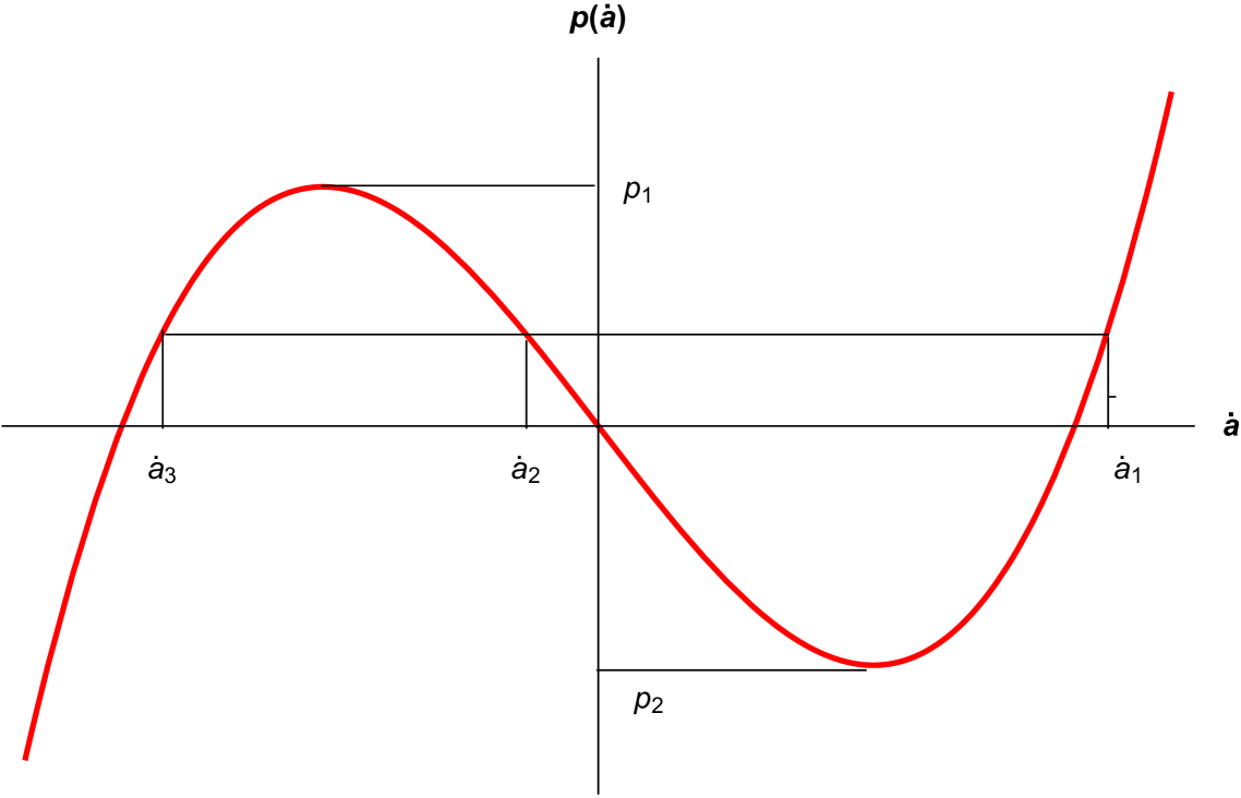
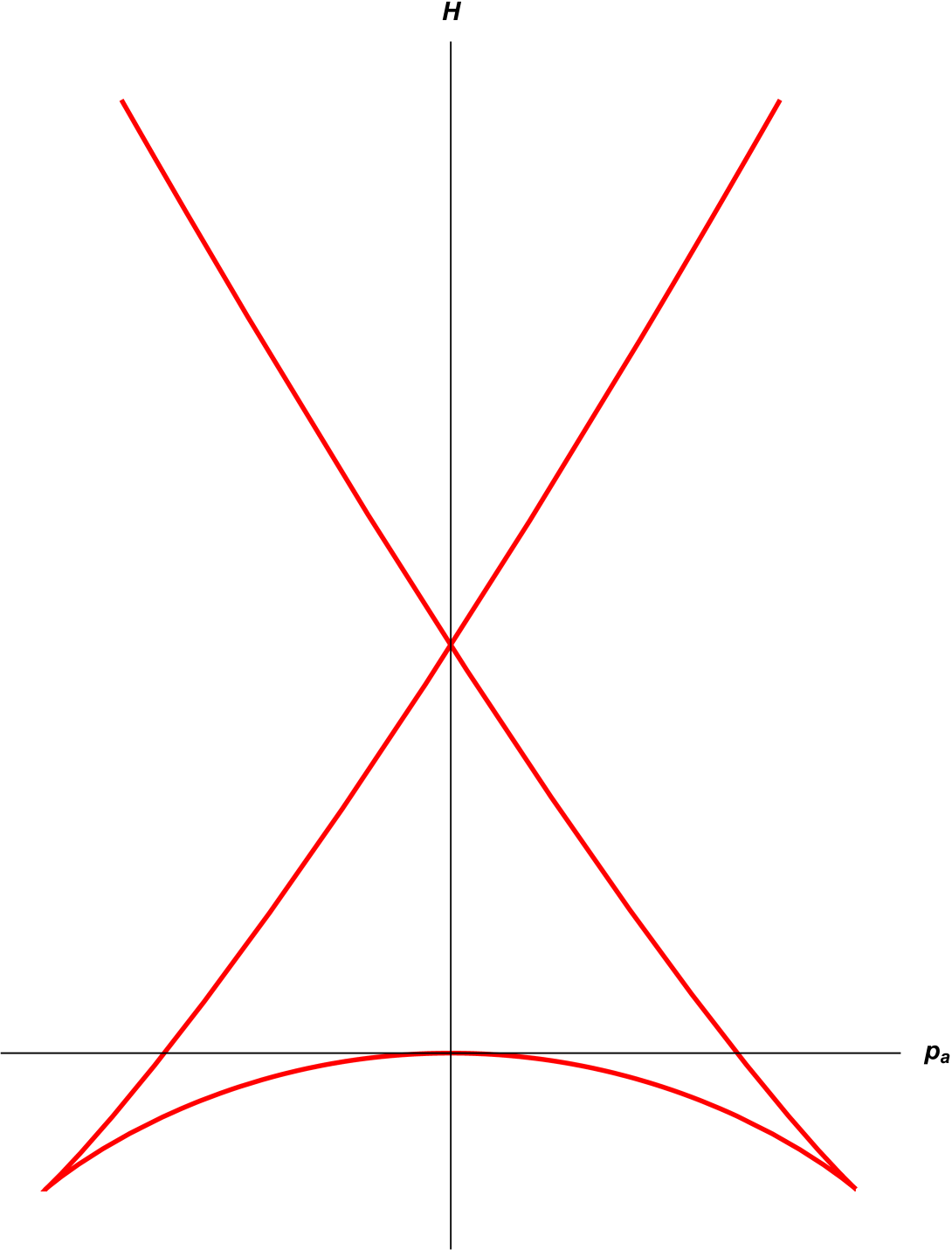
Fig-1 depicts that in the interval , the velocity is multi-valued and therefore it is not possible to predict the initial value of the momentum belongs to. As a result, the equations of motion switch or jump instantaneously from one value of the velocity to the another, because these instantaneous jumps leave unchanged and also satisfy the field equations. Further, Fig-2 suggests that or alternatively is also multi-valued and at any instant of time it is not possible to decide which ‘branch’ of the Hamiltonian one should use. Consequently, the associated field might propagate for a while with one choice of the Hamiltonian and then switch over to another and so on. Since such switching occurs within arbitrarily small intervals of time, the classical motion is visualized as a succession of irregular wiggles, which happens in an unanticipated manner. Hence, the behavior of the system described by the action (2) remains unpredictable for a range of initial non-vanishing data. Such a situation arises because the Lagrangian is quartic in the velocities and therefore expressions for velocities are multivalued functions of momentum, resulting in the so-called ‘multiply branched Hamiltonian’ with cusps (fig-2). Due to such jump from one branch of the Hamiltonian to the other at any instant of time, the classical solution remains unpredictable. Note that the presence of cusps restricts the domain of the variables.
The pathology of such ‘Branched Hamiltonian’ appears in different fields of physics and attempts to resolve the issue remains unsuccessful over decades. In the context of a toy model of Lanczos-Lovelock gravity in particular, it had been shown that different Hamiltonian emerges from different attempts made to circumvent the problem [45]. Nonetheless, in the absence of a viable unique theory, it had been shown that the pathology may be bypassed by adding a term in the Pais-Uhlenbeck oscillator action [46] and term in the Lanczos-Lovelock action, without any problem [45, 46, 47]. The same technique was adopted in theory of gravity [35]. It is to be mentioned that the issue of branching significantly depends on the choice of the signature of the parameters and and both are taken positive earlier arbitrarily [35]. While, the signature is fixed from the very beginning in the Pais-Uhlenbeck and the Lanczos-Lovelock actions, here for gravity, one needs to check the energy condition, which was not considered previously [35] based on earlier works [44]. This issue was recently sketched in a conference parer [48]. In the following, we consider it extensively in the context of energy condition to fix the signatures of and .
3.2 Energy conditions, the need for a scalar in the very early universe:
The energy conditions for has been studied recently in [43], where it has been revealed that one needs to fix and , if a minimally coupled scalar field is associated. Let us recall that the modified and alternative (teleparallel) theories of gravity are contemplated as alternatives to the uncanny dark energy and the motivation of these theories is to solve the cosmic puzzle in the late universe without dark energy. Now, after graceful exit from inflation, particles are produced and a hot big-bang era reincarnates. This is the epoch dominated by radiation. It may be possible that a tiny amount of scalar field remains in the radiation era too, which is redshifted away leaving no trace in the matter dominated era. However, a much stringent situation emerges, if the scalar field is completely wiped out in the process of producing particles, so that the radiation era consists of perfect fluid only (inclusive of dark matter). In that case, the energy density and the thermodynamic pressure are related by , in the present choice of unit . So, it is necessary to investigate the energy condition in the presence of a perfect fluid. It is noteworthy that for such a fluid are the conditions which satisfy all the four energy conditions. Under the choice , equations (6) and (7) read as,
| (12) |
Clearly and , ensures . We therefore replace by and by , where both and . Let us now inspect the pressure equation, which now reads as,
| (13) |
where, and , after the said replacement. Now, since in the expanding model, , so implies, , requiring . Thus for the choice , the condition finally requires , and a decelerated expansion is realizable, which is the viable cosmic evolution. Thus,the energy conditions fix the coupling constants and and the form we shall deal with is,
| (14) |
where, and . Now let us consider even early universe where inflation is driven by a scalar field having components and . In that case, the weak energy condition , since in the expanding model . Nonetheless, the strong energy condition reads as,
| (15) |
Clearly for a de-Sitter type solution , the Hubble parameter is slowly varying, while last term dominates, and strong energy condition appears to be violated. But that is not an issue, since it is possible for , which is the slow-roll condition.
In view of the energy conditions we now consider the form (14), in which both the parametric signatures of are now fixed, and muse on to the issue of ‘Branched Hamiltonian’ yet again. The Lagrangian, the momentum and the energy now read as,
| (16) |
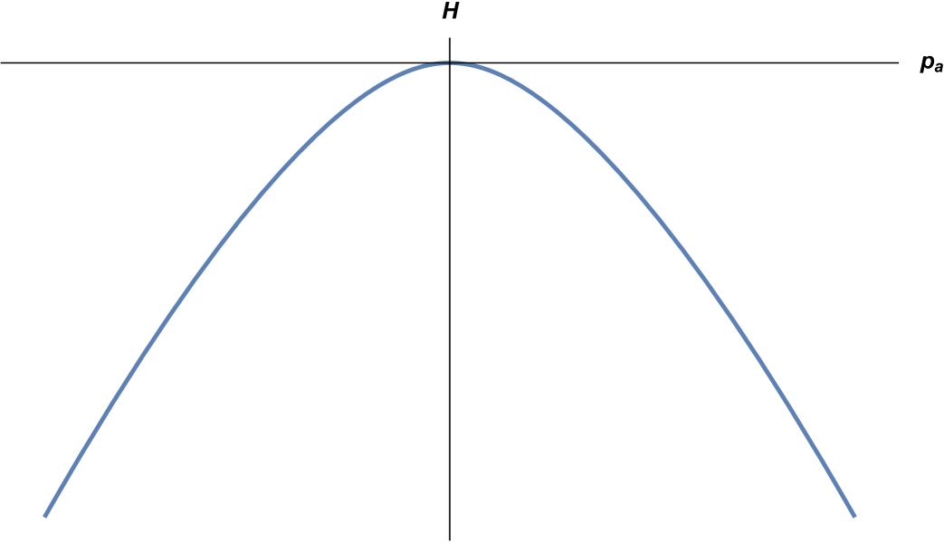
and as before, we present graphical representation of the momentum versus velocity and the Hamiltonian/Energy versus momentum as depicted below in fig-3 and fig-4. Clearly, the velocity as well as the Hamiltonian are now single valued and the pathology of Branched Hamiltonian disappears.

Thus, the restrictions of the energy condition resolves the pathology of branched hamiltonian. Now, considering the above form of , with proper sign of , the Einstein’s equation and the ‘’ variation are expressed in the presence of a scalar field as,
| (17) |
In the following subsection, we proceed to explore the inflationary regime.
3.3 Slow-roll inflation:
Before denying to work any further, the Planck satellite observations released a host of data sets imposing tighter constraint on the inflationary parameters, viz., on the spectral index as well as on the tensor to scalar ratio [49, 50]. More recently, combination of Planck PR4 data with ground-based experiments such as, BICEP/Keck 2018 (BK18), BAO and CMB lensing data, tightens the scalar to tensor ratio even further to [51]. Earlier as mentioned, scalar field driven inflation had been studied in the context of gravity with torsion, taking , in the background of RW metric [44] and for also for gravity with non-metricity in the background of anisotropic Bianchi-1 space-time for [43], and excellent agreement were found. Here, we consider () in the background of RW space-time for two different potentials, i) and ii) , unlike previous cases. Both these represent flat potentials, when becomes large enough on the onset of inflation. The field equations (17) now read as,
| (18) |
| (19) |
| (20) |
where the third equation is the variation equation. Applying the standard slow-roll conditions and , the equations (18) and (20) finally reduce to,
| (21) |
where . Solving for in view of (21), we propmtly obtain (considering the positive sign),
| (22) |
Further, combining equations (21) the slow-roll parameters are found as,
| (23) | ||||
where, the relation of comes from the equality between the ‘potential slow roll parameter’ and the ‘Hubble slow roll parameter’. Also, since in view of (18), one can also compute the number of e-folds as,
| (24) |
Case-1:
For the first choice of the potential, viz.,
| (25) |
the expressions of (23) and (24) are found as,
| (26) | ||||
The data set varying between , presented in Table-1, reveal that and lie very much within the experimental limit. As a result, the number of e-folds is found to vary within the range , which is sufficient to solve the horizon and flatness problems. Clearly, the agreement is outstanding, since the scalar to tensor ratio is able to sustain further constraints, which might appear from future analysis.
| in | in | |||
|---|---|---|---|---|
| 0.69953 | 0.40 | 0.96388 | 0.03224 | 44 |
| 0.69814 | 0.30 | 0.96402 | 0.03187 | 46 |
| 0.69692 | 0.20 | 0.96415 | 0.03154 | 48 |
| 0.69599 | 0.10 | 0.96425 | 0.03128 | 50 |
| 0.69586 | 0.08 | 0.96426 | 0.03124 | 51 |
| 0.69575 | 0.06 | 0.96427 | 0.03121 | 52 |
| 0.69561 | 0.01 | 0.96429 | 0.03117 | 53 |
| 0.69560 | 0.96430 | 0.03116 | 54 |
Next as an example, we compute the energy scale of inflation in view of the relation (22), selecting one of the data appearing in Table 1, viz., (, for which ), . Correspondingly, we find,
| (27) |
which is still arbitrary, since has not been fixed as yet. Now, the energy scale of inflation for a single scalar field model corresponding to GTR is given by the following relation [52],
| (28) |
In the above, we computed the numerical value taking into account the tensor-to-scalar ratio which appears for , under consideration (see Table 1). Other way round for a cross check, let us consider that inflation lasted for , i.e., it occurs between to , then for the same value of , which is precisely , . However, in our chose system of unit, . Hence, . Thus, to arrive that this scale of inflation, we need to constrain . Once the parameter is fixed from physical consideration (sub-Planckian scale of inflation), the values of and are found as well,
| (29) |
Finally, it is now required to check if graceful exit from inflation for the following model. We therefore recall equation (18), which in view of the above form of the potential, , is expressed as,
| (30) |
Initially, during inflation all the terms in (30) are more-or-less of the same order of magitude, since the is slowly varying. Nonetheless as inflation halts, the Hubble parameter falls of sharply and so one can neglect both the terms and appearing in the left hand side of (30) without any loss of generality to arrive at,
| (31) |
Taking into account, , and from Table-1, one can trivially exhibit the following oscillatory behavior of the scalar field at the end of inflation,
| (32) |
provided, , and hence graceful exit from inflation is exhibited.
Case-2:
Next, we consider yet another form of the potential, viz.,
| (33) |
Such a potential had been widely used to study inflation. This potential has excellent feature. The almost flat behaviour of the potential at the advent of inflation, when is large enough, allows slow roll to be conceivable. The expressions of (23) and (24) are now found as,
| (34) | ||||
In Table-2, we present a data set for the expressions (34), varying between . The result is, and lie very much within the experimental limit, while the variation of the number of e-folds , is not to large. Here again we find wonderful agrement with the Planck’s data, while the scalar to tensor ratio can confront further constraints, which as mentioned might appear from future analysis.
| in | in | |||
|---|---|---|---|---|
| 0.03928 | 8.0 | 0.96001 | 0.02440 | 71 |
| 0.03905 | 7.8 | 0.96004 | 0.02432 | 72 |
| 0.03862 | 7.4 | 0.96011 | 0.02414 | 73 |
| 0.03819 | 7.0 | 0.96018 | 0.02396 | 74 |
| 0.03777 | 6.6 | 0.96024 | 0.02378 | 75 |
| 0.03737 | 6.2 | 0.96031 | 0.02360 | 76 |
Let us also compute the energy scale of inflation in view of the relation (22), considering the data, (, for which ), appearing in Table 2. Correspondingly, we find,
| (35) |
which remains arbitrary unless is fixed. The energy scale of inflation in a single scalar field model corresponding to GTR [52], as already considered earlier, is given by the following expression,
| (36) |
whose numerical value is computed taking into account the value of the tensor-to-scalar ratio from the same data set () of Table 2 under consideration. Again as before taking and , one can compute . Thus, for the scale of inflation (35) is comparable with the single field scale of inflation (36). Since is fixed from physical consideration (sub-Planckian scale of inflation), the values of and may also be computed, which are,
| (37) |
Finally, to exhibit graceful exit from inflation, we recall equation (18), which in view of the above form of the potential, , is expressed as,
| (38) |
During inflation, is slowly varying and all the terms in (38) almost are of the same order of magnitude. However, as inflation ends the Hubble parameter decreases sharply, and so both the left hand side terms and may be neglected without loss of generality, to find,
| (39) |
Taking into account, , and from Table-2, it is possible to show that the above equation exhibits oscillatory behavior
| (40) |
provided, .
In a nut-shell, the inflationary parameters computed for the form , associated with the ‘metric’ as well as ‘symmetric’ teleparallel gravity theories are in excellent agreement with the observed inflationary parameters, for both the choice of potentials and .
3.4 Radiation era:
However, exhibiting a viable inflationary era is not enough. At the end of inflation, particles are produced giving way to the hot big-bang. Thereafter the universe enters the radiation dominated era, which is best described by the Friedmann-Lematre-like standard model solution , a decelerated expansion is amenable though. This subsection is therefore dedicated to unfurl the radiation era in the absence of the scalar field as well as in its little presence associated with the chosen forms of potentials. If the scalar field is completely used up in producing particles, then in is absence, eliminate from (17) one finds,
| (41) |
The above equation, upon integration gives,
| (42) |
The above equation indicates that for expanding universe , the second term dominates over the first, resulting in a negative . On the contrary, for positive this equation results a negative i.e contracting model. Clearly these are not viable.
Therefore, let us consider the presence of the scalar field, however small, so that the equations (17) now read as,
| (43) |
Combining the above pair of equations one obtains,
| (44) |
For a power law solution in the form , the (44) can be expressed as,
| (45) |
For both the forms of the potentials we found (31) and (39), i.e., at the end of inflation. Using this relation, the above equation is simplified to,
| (46) |
which is not satisfied in general. Nonetheless, radiation domination initiated at around and lasted till matter-radiation equality , while CMB formed at the decoupling era . Therefore, only at the very early stage , the first term is negligible inducing a coasting solution . However, soon as , the first term starts dominating leading to a viable radiation era , i.e., .
On the contrary, if we choose a-priori, then (45) takes the following form,
| (47) |
which for reduces to
| (48) |
and is satisfied for , i.e., , provided , resulting in . Undoubtedly, this is an awesome result, but then we need to check if the quartic potential is feasible in the inflationary era. This we compute briefly, next. One can find the expressions for and in view of equations (23) and (24) respectively as,
| (49) | ||||
In order to keep the scalar spectral index () and the scalar to tensor ratio within experimental limit and , usually has to be negative. However, here and so it has to be insignificantly small positive number. Even if, we take and use the the already fixed values of , then inflation ends () as . For this, the parametric values are computed as . Clearly, it is not possible to keep both the scalar-tensor ratio and the e-folding within the experimental limit simultaneously, if is fixed a-priori and vice-versa. In fact, Planck’s data rule out quartic potential and we also disregard it.
In a nut-shell, the form , associated with the ‘metric’ as well as ‘symmetric’ teleparallel gravity theories for both the choice of the potentials and admit a Friedmann-Lematre-like radiation era, apart from the very early phase. The fact that one cannot avoid the presence of the scalar field is apparent.
4 A more generalized form:
As mentioned, in the context of ‘metric teleparallel gravity’, it is suggested that a term solves the cosmic puzzle without dark energy, for . The term is included as a scale, so that as the Hubble parameter inflation is realized in the very early universe, while as late-time acceleration is achieved. However, we have noticed that vacuum teleparallel equations do not admit any viable form of unless an additional field, such as a scalar field is incorporated. The fact that a scalar field necessarily drives successful inflation has also been explored. The scale is therefore absolutely unnecessary, since any additional term should only be effective at the late-stage of cosmic evolution. We therefore simply consider an additional term such as , setting and inspect the consequence for . The generalized form is now . The field equations may therefore be written as,
| (50) |
First of all note that if we choose , then the first equation of (50) is never satisfied for any arbitrary . As a result a viable (decelerated) radiation as well as early matter dominated eras are not realizable under any circumstances. As already noticed, the presence of a scalar field, however small, can only produce a decelerated Friedmann-like radiation era, in the absence of the last term. Let us therefore concentrate on the late-stage of matter (pressureless dust) dominated era.
For , . But from the second equation of (50) one can observe that as the Hubble parameter decreases, the third term on the left hand side starts dominating and as a result . While for exponential expansion , resulting in . Clearly a perfect fluid source is absolutely incredible to solve the cosmic puzzle.
On the contrary, for , where , until is not too small, so that . Also up to the said limit. Thus, energy conditions are satisfied till . But no analytical solution possibly exist. Summarily, without associating an additional field teleparallel gravity theories neither can engender a feasible radiation as well as an early matter dominated eras nor can combat the cosmic puzzle.
5 Concluding remarks:
Although, perturbative analysis results in serious pathologies of generalized teleparallel gravity theories in flat space, nonetheless, these may be outcome of first-order analysis. The theory is still open until higher-order perturbative analysis is performed. In the present article, we closely inspect some features and credentials of both the teleparallel gravity theories. Summarily, we take generalized ‘torsion’ as well as ‘non-mtricity’ (in coincidence gauge) teleparallel gravity theories on the same footing in the background of isotropic and homogeneous Robertson-Walker metric and consider a generic generalized form . At the beginning, we exhibited the fact that the vacuum era does not admit any viable generalized form, unless it is accompanied with an additional field. As a result, unlike ‘curvature induced inflation’, ‘torsion’ or ‘non-metricity’ induced inflation is obscure. Next we choose a form of , as a minimal modification from ‘GTR’ and in view of the energy conditions, find . This banishes the pathology of ’Branch Hamiltonian’ publicized earlier taken into account . Inflation driven by a scalar field with was also studied and excellent agreement with the latest released Planck’s data set was found. It is therefore necessary to study the same for , as well. This is also done for two different potentials and . The inflationary parameters, viz., the ‘scalar to tensor ratio (), the ‘spectral index ()’ and the ‘number of e-folds () are found to agree quite appreciably with the recently released Planck’s data for the standard choice . The parameter is fixed comparing with the energy scale of single-field inflation in GTR and the theory is found to exit gracefully from inflation. In the absence of a scalar field a viable radiation era is inconceivable. On the contrary, considering the presence of a little bit of scalar field, it is found that apart from the very early coasting solution , both the potentials give rise to the FLRW-like radiation era . So far so good, but finally it is found that a viable (decelerated) early matter dominated era as well late stage of cosmic acceleration compel the presence of an additional field. In a nut-shell, teleparallel gravity theories (alone) are incompatible to expatiate any stage of the history of cosmic evolution without associating an extra field. This goes against the very first motivation for introducing these theories.
References
- [1]
- [2] A.Unzicker and T. Case, Translation of Einstein’s attempt of a unified field theory with teleparallelism, arXiv:physics/0503046 (2005).
- [3] G.R. Bengochea, Observational information for theories and Dark Torsion, Phys. Lett. B 695, 405-411 (2011), arXiv:1008.3188.
- [4] G.R. Bengochea and R. Ferraro, Dark torsion as the cosmic speed-up, Phys. Rev. D 79, 124019 (2009).
- [5] E.V. Linder, Einstein’s other gravity and the acceleration of the universe, Phys. Rev. D 81, 127301 (2010).
- [6] R.P. Woodard, The theorem of Ostrograafsky, Scholarpedia 10 (8) 32243 (2015), arXiv :1506.02210[hep -th].
- [7] K. Bamba, C.Q. Geng, C.C. Lee and L.W. Luo, Equation of state for dark energy in gravity, JCAP, 1101, 021 (2011).
- [8] K. Bamba, C.Q. Geng and C.C. Lee, Comment on “Einstein’s Other Gravity and the Acceleration of the Universe”, arXiv:1008.4036 [astro-ph.CO] (2010).
- [9] S.A. Narawade, L. Pati, B.Mishra and S.K. Tripathy, Dynamical system analysis for accelerating models in non-metricity gravity, Physics of the Dark Universe 36, 101020 (2022).
- [10] F.K. Anagnostopoulos, S. Basilakos, and E.N. Saridakis, First evidence that non-metricity f(Q) gravity can challenge CDM, Phys. Letts. B, 822 (2021), arxiv: 2104.15123.
- [11] R. Solanki, A. De, S. Mandal and P.K.Sahoo, Accelerating expansion of the universe in modified symmetric teleparallel gravity, Phys. Dark Univ., 36, 101053 (2022).
- [12] R. Solanki, A. De and P.K. Sahoo, Complete dark energy scenario in gravity, Phys. Dark Univ., 36, 100996 (2022).
- [13] L. Atayde and N. Frusciante, Can gravity challenge CDM?, Phys. Rev. D, vol. 104, no. 6, p. 064052 (2021).
- [14] B. Li, T.P. Sotiriou and J.D. Barrow, gravity and local Lorentz invariance, Phys. Rev. D 83, 064035 (2011).
- [15] A. Golovnev, Issues of Lorentz-invariance in gravity and calculations for spherically symmetric solutions, Class. Quantum Grav. 38, 197001 (2021).
- [16] J.B. Jimenez, L. Heisenberg and T.S. Koivisto, The Geometrical Trinity of Gravity, Universe 5(7), 173 (2019).
- [17] F. D’Ambrosio, L. Heisenberg and S. Kuhn, Revisiting Cosmologies in Teleparallelism, Class. Quantum Grav. 39, 025013 (2022).
- [18] J. Lu, Y. Guo and G. Chee, From GR to STG - Inheritance and development of Einstein’s heritages, arXiv:2108.06865 (2021).
- [19] S. Capozziello, V. De Falco and C. Ferrara, Comparing Equivalent Gravities: common features and differences, arXiv:2208.03011 [gr-qc] (2022).
- [20] A. De, S. Mandal, J.T. Beh, T.H. Loo and P.K. Sahoo, Isotropization of locally rotationally symmetric Bianchi-I universe in -gravity, Eur. Phys. J. C. 82, 72 (2022).
- [21] J.B. Jimenez, L. Heisenberg and T. Koivisto, Coincident General Relativity, Phys. Rev. D 98, 044048 (2018).
- [22] D. Zhao, Covariant formulation of theory, Eur. Phys. J. C 82, 303 (2022).
- [23] R. H. Lin and X. H. Zhai, Spherically symmetric configuration in gravity, Phys. Rev. D 103, 124001 (2021).
- [24] S. Mandal, D. Wang and P.K. Sahoo, Cosmography in gravity, Phys. Rev. D 102, 124029 (2020).
- [25] A. De and L.T. How, Comment on ‘Energy conditions in gravity’, Phys. Rev. D, 106, 048501 (2022).
- [26] N. Frusciante, Signatures of -gravity in cosmology, Phys. Rev. D 103, 0444021 (2021).
- [27] B.J. Barros, T. Barreiro1, T. Koivisto and N.J. Nunes, Testing gravity with redshift space distortions, Phys. Dark Univ. 30, 100616 (2020).
- [28] W. Khyllep, A. Paliathanasis and J. Dutta, Cosmological solutions and growth index of matter perturbations in gravity, Phys. Rev. D 103, 103521 (2021).
- [29] J. Lu, X. Zhao and G. Chee, Cosmology in symmetric teleparallel gravity and its dynamical system, Eur. Phys. J. C, 79, 530 (2019).
- [30] M. Li, H. Rao and D. Zhao, A simple parity violating gravity model without ghost instability, JCAP 11, 023 (2020).
- [31] M. Hohmann and C. Pfeifer, Teleparallel axions and cosmology, Eur. Phys. J. C, 81, 376 (2021).
- [32] J.B. Jiménez, L. Heisenberg, T. Koivisto and S. Pekar, Cosmology in f(Q) geometry, Phys. Rev. D 101, 103507 (2020), arXiv:1906.10027v2 [gr-qc].
- [33] J.B. Jiménez and T.S. Koivisto, Accidental gauge symmetries of Minkowski spacetime in Teleparallel theories, arXiv:2104.05566v2 [gr-qc].
- [34] D.A. Gomes, J.B. Jiménez, A.J. Cano and T.S. Koivisto, On the pathological character of modifications to Coincident General Relativity: Cosmological strong coupling and ghosts in f(Q) theories, arXiv:2311.04201v1 [gr-qc].
- [35] M. Chakrabortty, K. Sarkar and A.K. Sanyal, The issue of Branched Hamiltonian in Teleparallel Gravity, IJMPD, 31, 2250083 (2022), arXiv:2201.08390 [gr-qc].
- [36] A.A. Starobinsky, A new type of cosmological models without singularity, Phys. Lett. B 91, 99 (1980).
- [37] R. Myrzakulov, Accelerating universe from F(T) gravity. Eur. Phys. J. C 71, 1752 (2011), arXiv:1006.1120.
- [38] K. Bamba, S. Nojiri and S.D. Odintsov, Trace-anomaly driven inflation in f(T) gravity and in minimal massive bigravity. Phys. Lett. B 731, 257 (2014), arXiv:1401.7378.
- [39] G.G.L. Nashed, W.El Hanafy and Sh.Kh. Ibrahim, Graceful Exit Inflation in f(T) Gravity, arXiv:1411.3293v2.
- [40] V.K. Oikonomou, On the Viability of the Intermediate Inflation Scenario with F(T) Gravity, Phys. Rev. D 95, 084023 (2017) arXiv:1703.10515.
- [41] A. Awad, W. El Hanafy, G.G.L. Nashed, S.D. Odintsov and V.K. Oikonomou, Constant-roll Inflation in f(T) Teleparallel Gravity, JCAP 1807 (2018) 026, arXiv:1710.00682v3.
- [42] H.F. Abadji, M.G. Ganiou, M.J.S. Houndjo and J. Tossa, Inflationary scenario driven by type IV singularity in f(T) gravity, arXiv:1905.00718.
- [43] A. De, D. Saha, G.Subramaniam and A.K. Sanyal, Probing symmetric teleparallel gravity in the early universe, MPLA 2450071 (2024) arXiv:2209.12120 [gr-qc].
- [44] M. Chakrabortty, N. Sk, S. Sanyal and A.K. Sanyal, Inflation with teleparallel gravity, Eur. Phys. J. Plus, 136 1213 (2021), arXiv:2112.09609.
- [45] S. Ruz, R. Mandal, S. Debnath and A.K. Sanyal, Gen. Relativ. Gravit. 48,86 (2016), arXiv:1409.7197[hepth].
- [46] K. Sarkar, N. Sk, R. Mandal and A.K Sanyal, Canonical formulation of Pais-Uhlenbeck action and resolving the issue of branched Hamiltonian, International Journal of Geometric Methods in Modern Physics, 14, (2017) 1750038, arXiv:1507.03444v3 [hep-th].
- [47] S. Debnath, S. Ruz, R. Mandal and A.K. Sanyal, History of cosmic evolution with modified Gauss-Bonnet- dilatonic coupled term, Eur. Phys. J. C 77, 318 (2017).
- [48] D. Saha, A.K. Sanyal, Teleparallel gravity does not suffer from the Catastrophe of Branching, Ideal International E-Publication Pvt. Ltd.(ISBN: ), PROCEEDINGS OF INTERNATIONAL CONFERENCE on “Recent Trends in Physics and Allied Sciences”, 2023.
- [49] Y. Akrami et al. (Planck Collaboration), Planck 2018 results. X. Constraints on inflation, Astronomy & Astrophysics, 641, A10 (2020), arXiv:1807.06211 [astro-ph.CO].
- [50] N. Aghanim et al, Planck 2018 Results. VI. Cosmological Parameters, (Planck Collaboration), Astronomy & Astrophys., 641, A6 (2020), arXiv:1807.06209.
- [51] M. Tristram et al., Improved limits on the tensor-to-scalar ratio using BICEP and Planck, Phys. Rev. D 105 083524 (2022), arXiv: 2112.07961.
- [52] K. Enqvist, R.J. Hardwick, T. Tenkanen, V. Venninb and D. Wands, A novel way to determine the scale of inflation, JCAP, 02, 006 (2018), arXiv:1711.07344 [astro-ph.CO].