Don’t Fear Peculiar Activation Functions: EUAF and Beyond

Abstract

In this paper, we propose a new super-expressive activation function called the Parametric Elementary Universal Activation Function (PEUAF). We demonstrate the effectiveness of PEUAF through systematic and comprehensive experiments on various industrial and image datasets, including CIFAR10, Tiny-ImageNet, and ImageNet. Moreover, we significantly generalize the family of super-expressive activation functions, whose existence has been demonstrated in several recent works by showing that any continuous function can be approximated to any desired accuracy by a fixed-size network with a specific super-expressive activation function. Specifically, our work addresses two major bottlenecks in impeding the development of super-expressive activation functions: the limited identification of super-expressive functions, which raises doubts about their broad applicability, and their often peculiar forms, which lead to skepticism regarding their scalability and practicality in real-world applications.

[inst1]organization=Center of Mathematical Artificial Intelligence,addressline=Department of Mathematics, city=The Chinese University of Hong Kong, state=Hong Kong, country=China [inst2]addressline=Department of Applied Mathematics, city=The Hong Kong Polytechnic University, state=Hong Kong, country=China [inst3]addressline=Department of Biomedical Engineering, city=Southern Medical University, state=Guangzhou, country=China [inst4]organization=Institute of Medical Technology,addressline=Peking University Health Science Center, city=Peking University, state=Beijing, country=China [inst5]organization=Independent Researcher,addressline=708 6th Ave N, Seattle, WA 98109, US

1 INTRODUCTION

In recent years, deep learning has achieved significant success in many critical areas (LeCun et al., 2015). A major factor contributing to this success is the development of highly effective nonlinear activation functions, which greatly enhance the information processing capabilities of neural networks. While established options like the Rectified Linear Unit (ReLU) and its variants are widely used (Nair and Hinton, 2010), the fundamental importance of activation functions makes the search for better ones a continuous effort. Researchers are persistently working to design and evaluate various activation functions through both theoretical analysis and empirical studies (Bingham and Miikkulainen, 2022; Apicella et al., 2021; Wang et al., 2024).

In the realm of approximation theory, it has been shown that certain activation functions can empower a neural network with a simple structure to approximate any continuous function with an arbitrarily small error, using a fixed number of neurons (Maiorov and Pinkus, 1999). These functions are termed “super-expressive activation functions” (Yarotsky, 2021). According to research, to achieve super-expressiveness, an activation function should possess both periodic and analytical components (Shen et al., 2022; Yarotsky, 2021). One such example is the elementary universal activation function (EUAF), defined as follows:

$$\mathrm{EUAF}(x)\coloneqq\begin{cases}\big{|}x-2\lfloor\tfrac{x+1}{2}\rfloor\big{|}&\text{for}\ x\geq 0,\\ \frac{x}{1+|x|}&\text{for}\ x<0,\\ \end{cases}$$

Figure 1 depicts EUAF, an analytical function on $(-\infty,0)$ and periodic on $[0,\infty)$. The unique and highly desirable property of super-expressiveness allows neural networks to achieve precise approximation accuracy without increasing network complexity. This contrasts with traditional universal approximation methods, where more complex structures and a higher number of neurons are required as the approximation error decreases. By integrating super-expressive activation functions, one can attain the desired approximation accuracy by merely adjusting parameters, thus maintaining a simpler network architecture.

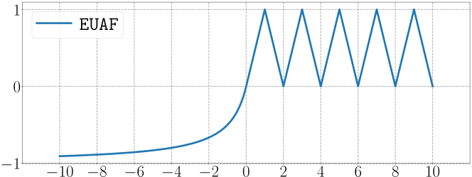
Figure 1: An illustration of $\mathrm{EUAF}$.

To the best of our knowledge, the development of super-expressive activation functions faces two technical challenges that hinder their potential value to neural networks: 1) First, only a limited number of super-expressive functions have been identified so far  (Maiorov and Pinkus, 1999; Shen et al., 2022; Yarotsky, 2021). It is unclear if the super-expressive property can be broadly applied. Additionally, for deep learning practitioners, having a greater variety of activation functions that exhibit learning capabilities is necessary in terms of enriching their armory. Developing more super-expressive functions increases the likelihood of finding their utilities in important applications, as different activation functions differ in their trainability. 2) Second, the practical utility of super-expressive activation functions is questionable. While superior expressiveness can be theoretically established through specialized constructions that demonstrate the existence of an expressive solution  (Shen et al., 2021; Yarotsky, 2021), this does not necessarily translate to better practical performance. Furthermore, it is unclear whether gradient-based methods can effectively learn good solutions for networks using these functions.

Compared to commonly used functions like ReLU, sigmoid, and tanh, super-expressive functions usually have peculiar shapes. For example, Figure 1 shows EUAF, which is a typical super-expressive activation function. It has a complex and intimidating form, which makes most practitioners skeptical about its scalability and practicality in real-world applications. If we can demonstrate the practical utility of any super-expressive activation function, it could help resolve the skepticism and bridge the gap between their theoretical elegance and usefulness.

In addressing the first bottleneck, we substantially generalize the scope of EUAF to encompass a large family of functions capable of achieving super-expressiveness. Specifically, an activation function $\rho$ is considered to be super-expressive if it is real analytic within a small interval and a fixed-size $\rho$-activated network can reproduce a triangle-wave function. To address the second bottleneck, we believe that super-expressive functions can indeed be practically useful. Previous studies  (Sitzmann et al., 2020; Ramirez et al., 2023) successfully applied the periodic function sin as an activation function within the implicit neural representation. These models have been demonstrated to be suitable for representing complex signals and their derivatives, as well as for solving challenging boundary value problems  (Liu et al., 2022a). These studies provide valuable insights into the potential of super-expressive activation functions, since both super-expressive activation functions and sin share periodicity. Moreover, from the perspective of signal decomposition, normal activation functions like ReLU tend to assist models in identifying the direct component (DC) of a signal  (Lee et al., 2024). In contrast, super-expressive activation functions can better handle stationary signals due to their inherent periodicity. This characteristic enhances their ability to manage complex real-world signals more efficiently.

Specifically, we choose EUAF as our representative and investigate a parameterized variant, named PEUAF, which adaptively learns the frequency $w$ on the positive side. Mathematically,

$$\mathrm{PEUAF}(x)\coloneqq\begin{cases}\big{|}wx-2\lfloor\tfrac{wx+1}{2}\rfloor\big{|}&\textnormal{for}\ x\geq 0,\\ \frac{x}{1+|x|}&\textnormal{for}\ x<0,\\ \end{cases}$$

where $w$ is the trainable parameter representing the frequency on the positive side. PEUAF can adaptively extract the stationary signals with different frequencies. This adaptability allows PEUAF to effectively capture and represent signals with diverse frequency components, which is particularly advantageous in addressing real-world signal complexities. Then, we validate the effectiveness of PEUAF by experimenting with four industrial datasets (1D data) and three image datasets (2D data). For industrial datasets, our tests show that PEUAF surpasses other activation functions in terms of test accuracy, convergence speed, and fault localization ability. For image datasets, we find that combining PEUAF with other activation functions can usually yield better performance than only using a single activation function, although using PEUAF alone cannot achieve satisfactory performance. Thus, PEUAF can serve as a valuable add-on to the network. Our main contributions are as follows:

• We provide a non-trivial generalization of EUAF, showing that a broader family of activation functions can achieve super-expressiveness.

• We bridge the gap between the theoretical elegance and empirical usefulness of super-expressive functions by demonstrating their competitive performance in practical applications through systematic experiments on four industrial datasets and three image datasets including ImageNet.

• We introduce PEUAF, a parameterized version of EUAF, and demonstrate that PEUAF can be used individually or in conjunction with other well-performing activation functions.

2 RELATED WORK

In the field of artificial intelligence, deep neural networks have proven to be highly effective tools. These networks leverage the power of interconnected nodes structured in multiple layers, allowing them to excel in a wide range of complex applications and new domains. At their core, deep neural networks rely on an affine linear transformation followed by a nonlinear activation function. The nonlinear activation function is essential for the successful training of these networks.

Later in this section, we will first review conventional activation functions including ReLU and its variants, as well as recent sigmoidal activation functions in Section 2.1. We will then discuss super-expressive activation functions in Section 2.2.

2.1 Conventional Activation Functions

In recent years, the Rectified Linear Unit (ReLU (Nair and Hinton, 2010)), defined as $\texttt{ReLU}(x)=\max(0,x)$, has gained popularity and recognition for its effectiveness in addressing the gradient vanishing and explosion issues encountered with Sigmoid and Tanh activation functions. Thus, ReLU has been widely used in the deep learning community such as industrial fault diagnosis (Liu et al., 2024a) and medical image segmentation (Liu et al., 2024b) . However, ReLU can suffer from the occurrence of a number of “dead neurons”, which results in information loss and can hurt the neural network’s feature processing ability. To mitigate this issue, several variants of ReLU have been introduced such as Leaky Rectified Linear Unit (LReLU)  (Xu et al., 2015), Parametric Rectified Linear Unit (PReLU)  (He et al., 2015), Randomized Leaky Rectified Linear Unit (RReLU)  (Xu et al., 2015), Exponential Linear Unit (ELU)  (Clevert et al., 2015), Gaussian Error Linear Unit (GELU)  (Hendrycks and Gimpel, 2016), and Generalized Linear Unit (GENLU)  (Fan et al., 2020). Most recently, Goldenstein et al. (2024) proposed Self-Normalizing ReLU or NeLU to ensure that the prediction model is not affected by the noise level during testing. It has been tested in synthetic data and image de-noising tasks. These variants represents a significant advancement in activation function design, offering adaptability and potentially better performance. Whereas, their benefits come with the cost of increased model complexity or computation burden and the need for careful tuning and regularization which inspired researchers to create more different activation functions.

In addition to these ReLU variants, other kinds of activation functions have also been developed. For example, the Swish ($\mathrm{Swish}(x)=x\cdot\mathrm{sigmoid}(\beta x)$)  (Ramachandran et al., 2017) was identified through an automated search using a combination of exhaustive and reinforcement learning as an alternative to ReLU. Its similar shape makes it a reasonable proxy for ReLU in deep learning applications. Mish, defined as $\mathrm{Mish}(x)=x\cdot\mathrm{tanh}(\mathrm{softplus}(x))$  (Misra, 2020), exhibits superior empirical results compared to ReLU, Swish, and LReLU in CIFAR-10 and ImageNet classification tasks. Fractional adaptive linear units FALUs (Zamora et al., 2022) incorporate fractional calculus principles into activation functions, thereby defining a diverse family of activation functions. It has demonstrated enhanced performance in image classification tasks, improving test accuracy. The Seagull activation function, introduced by  (Gao and Zhang, 2023), stands out as a customized activation function designed for applications in regression tasks featuring a partially exchangeable target function. It exhibits superiority in addressing the specific demands of regression scenarios.

Overall, the above-mentioned activation functions are hard to be generalized across different domains, especially in industrial applications. Another problem is that the lack of theoretical analysis limits the acceptance of these activation functions in spite of their good performance. Therefore, it is necessary to verify an activation function with a good theoretical guarantee.

2.2 Super-Expressive Activation Functions

Numerous studies have explored new activation functions to make a fixed-size network achieve an arbitrary error, referred to as super-expressive activation functions. For example, Maiorov and Pinkus (1999) proposed an activation function to achieve this goal, but it lacks a closed form and is computationally impractical. Recently, Yarotsky (2021) demonstrated that simple functions such as $(\texttt{sin},\texttt{arcsin})$ can achieve super-expressiveness, although the relationship between the network size and the dimension was unclear. However, despite the above problems, sin has been proven to be effective in 3D neural network field, indicating the potential of super-expressiveness in neural networks (Ramirez et al., 2023). Shen et al. (2022) proposed EUAF, showing that a network with EUAF requires only $\mathcal{O}(d^{2})$ width and $\mathcal{O}(1)$ depth to achieve super-expressiveness. The potential of EUAF is demonstrated among simple experiments such as function approximation and Fashion-MNIST classification. They also explored the approximation of a neural network with three hidden layers which is named Floor-Exponential-Step (FLES) networks (Shen et al., 2021). The utilized floor function ($\left\lfloor x\right\rfloor$) can be recognized as an activation function with super-expressiveness (Yarotsky, 2021). In a word, these super-expressive activation functions play a theoretically pivotal role in endowing models with the universal approximation property for all continuous functions. However, previous research either lacked experiments or only included simple ones, leaving it unknown whether these super-expressive functions are practically valuable.

3 Enriching the Family of Super-expressive Activation Functions

In this section, we aim to significantly expand the scope of EUAF activation function by introducing a comprehensive collection of activation functions, each with approximation properties akin to those of EUAF. For simplicity, let ${\hskip 0.6pt\mathcal{N}\mathcal{N}}_{\varrho}\{N,\hskip 1.987ptL;\hskip 3.0297pt{{\mathbb{R}}^{d}}\to{{\mathbb{R}}^{n}}\}$ denote the set of neural networks $\phi:{\mathbb{R}}^{d}\to{\mathbb{R}}^{n}$ that can be represented by $\varrho$-activated networks, with a maximum width of $N$ and a maximum depth of $L$. Let ${\mathscr{A}}$ represent the set of all super-expressive activation functions $\varrho:{\mathbb{R}}\to{\mathbb{R}}$, which satisfy the following conditions:

• There exists an interval $(\alpha,\beta)$ with $\alpha<\beta$ where $\varrho$ is real analytic and non-polynomial on $(\alpha,\beta)$.

• There exists a fixed-size $\varrho$-activated network $\phi$ that can reproduce a triangle-wave function on $[0,\infty)$, i.e.,

  $$\phi(x)=\big{|}x-2\big{\lfloor}\tfrac{x+1}{2}\big{\rfloor}\big{|} {\forall\,}x\in[0,\infty)$$  .

We denote ${\overline{\mathscr{A}\,\!}}$ as the “closure” of ${\mathscr{A}}$. This means a function $\varrho$ is in ${\overline{\mathscr{A}\,\!}}$ if and only if, for any $A>0$ and $\varepsilon>0$, there exists a $\varrho_{\varepsilon}\in{\mathscr{A}}$ such that:

$$|\varrho_{\varepsilon}(x)-\varrho(x)|<\varepsilon\quad{\forall\,}x\in[-A,A].$$

Theorem 1.

Given any $\varrho\in{\overline{\mathscr{A}\,\!}}$, the hypothesis space

$${\hskip 0.6pt\mathcal{N}\mathcal{N}}_{\varrho}\big{\{}{\mathcal{O}}(d^{2}),\hskip 1.987pt{\mathcal{O}}(1);\hskip 3.0297pt{{\mathbb{R}}^{d}}\to{{\mathbb{R}}}\big{\}}$$

is dense in $C([a,b]^{d})$ in terms of the supremum norm.

It is crucial to highlight that the constants in the ${\mathcal{O}}(\cdot)$ notation in Theorem 1 can be explicitly determined and depend only on the choice of $\varrho$. The proof of Theorem 1 will be provided later in this section.

Before giving the proof, let us provide several examples in ${\overline{\mathscr{A}\,\!}}$. The first example, $\varrho_{1}\in{\overline{\mathscr{A}\,\!}}$, exhibits an S-shape and is defined as follows:

$$\varrho_{1}\coloneqq\begin{cases}\frac{x}{1-x}&\textnormal{for}\ x\leq 0,\\ \tfrac{x}{1+x}+\frac{g(x)}{x^{2}+10}&\textnormal{for}\ x>0,\\ \end{cases}$$

where $g(x)=\big{|}x-2\big{\lfloor}\tfrac{x+1}{2}\big{\rfloor}\big{|}$ for any $x\in{\mathbb{R}}$.

The second example, $\varrho\in{\overline{\mathscr{A}\,\!}}$, resembles the ReLU activation function and is defined as follows:

$$\varrho_{2}\coloneqq\begin{cases}0&\textnormal{for}\ x\leq 0,\\ x+\frac{g(x)}{x+1}&\textnormal{for}\ x>0.\\ \end{cases}$$

The third example, $\varrho_{1}\in{\mathscr{A}}\subseteq{\overline{\mathscr{A}\,\!}}$, is defined as follows:

$$\varrho_{3}\coloneqq\begin{cases}\tfrac{2}{\pi}\arcsin(x)&\textnormal{for}\ -1\leq x\leq 1,\\ \sin(\tfrac{\pi}{2}x)&\textnormal{for}\ |x|>1.\\ \end{cases}$$

See Figure 2 for visual representations of $\varrho_{1}$, $\varrho_{2}$, and $\varrho_{3}$.

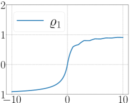
(a)

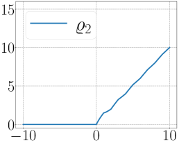
(b)

(c)

Figure 2: Illustrations of $\varrho_{1}$, $\varrho_{2}$, and $\varrho_{3}$.

Now, we will focus on proving the validity of Theorem 1. Given any any $f\in C([a,b]^{d})$ and $\varepsilon>0$, our goal is to construct $\phi\in{\hskip 0.6pt\mathcal{N}\mathcal{N}}_{\varrho}\{{\mathcal{O}}(d^{2}),\hskip 1.987pt{\mathcal{O}}(1);\hskip 3.0297pt{{\mathbb{R}}^{d}}\to{{\mathbb{R}}^{n}}\}$ such that

$$|\phi({\bm{x}})-f({\bm{x}})|<\varepsilon\quad{\forall\,}{\bm{x}}\in[a,b]^{d}.$$

Several concepts used to establish Theorem 1 can be traced back to the research conducted by (Shen et al., 2022) and (Yarotsky, 2021). The proof can be divided into three main steps as follows.

• The primary objective of the first step is to create a neural network that effectively approximates the univariate function $f\in C([0,1])$ within a specific “half” interval.

  Theorem 2.

  Given any $f\in C([0,1])$, $\varrho\in{\overline{\mathscr{A}\,\!}}$, $\varepsilon>0$, and $K\in{\mathbb{N}}$, suppose for any $x_{1},x_{2}\in[0,1]$, it holds that

  $$|f(x_{1})-f(x_{2})|<\varepsilon/2\ \textnormal{ if $|x_{1}-x_{2}|<1/K$.}$$ (1)

  Then there exists $\phi\in{\hskip 0.6pt\mathcal{N}\mathcal{N}}_{\varrho}\{{\mathcal{O}}(1),\hskip 1.987pt{\mathcal{O}}(1);\hskip 3.0297pt{{\mathbb{R}}}\to{{\mathbb{R}}}\}$ such that

  $$|\phi(x)-f(x)|<\varepsilon\quad\textnormal{for any}\ x\in\bigcup_{k=0}^{K-1}\big{[}\tfrac{2k}{2K},\tfrac{2k+1}{2K}\big{]}.$$

• The second step’s aim is to utilize the outcome of the first step, Theorem 2, to build a network that effectively approximates the function $f\in C([a,b])$ within the entire interval $[a,b]$.

  Theorem 3.

  Given any $f\in C([a,b])$, $\varrho\in{\overline{\mathscr{A}\,\!}}$, and $\varepsilon>0$, there exists $\phi\in{\hskip 0.6pt\mathcal{N}\mathcal{N}}_{\varrho}\{{\mathcal{O}}(1),\hskip 1.987pt{\mathcal{O}}(1);\hskip 3.0297pt{{\mathbb{R}}}\to{{\mathbb{R}}}\}$ such that

  $$|\phi(x)-f(x)|<\varepsilon\quad\textnormal{for any $x\in[a,b]$.}$$

• The ultimate objective of the final step is to generalize the one-dimensional findings described in Theorem 3 to the multi-dimensional scenario. To achieve this, we will utilize Kolmogorov’s superposition theorem (KST) (Kolmogorov, 1957), summarized in Theorem 4. It is important to note that the target function $f\in C([a,b]^{d})$ can be appropriately rescaled to facilitate the application of KST.

  Theorem 4 (KST).

  There exist continuous functions $h_{i,j}\in C([0,1])$ for $i=0,1,\mathinner{\mkern-0.1mu\cdotp\mkern-0.3mu\cdotp\mkern-0.3mu\cdotp\mkern-0.1mu},2d$ and $j=1,2,\mathinner{\mkern-0.1mu\cdotp\mkern-0.3mu\cdotp\mkern-0.3mu\cdotp\mkern-0.1mu},d$ such that any continuous function $f\in C([0,1]^{d})$ can be represented as

  $$f({\bm{x}})=\sum_{i=0}^{2d}g_{i}\Big{(}\sum_{j=1}^{d}h_{i,j}(x_{j})\Big{)}$$

  for any ${\bm{x}}=(x_{1},\mathinner{\mkern-0.1mu\cdotp\mkern-0.3mu\cdotp\mkern-0.3mu\cdotp\mkern-0.1mu},x_{d})\in[0,1]^{d}$, where $g_{i}:{\mathbb{R}}\to{\mathbb{R}}$ is a continuous function for each $i\in\{0,1,\mathinner{\mkern-0.1mu\cdotp\mkern-0.3mu\cdotp\mkern-0.3mu\cdotp\mkern-0.1mu},2d\}$.

We observe that it is sufficient to demonstrate the case where $\varrho\in{\mathscr{A}}$ rather than $\varrho\in{\overline{\mathscr{A}\,\!}}$, aided by the following lemma.

Lemma 1 (Proposition 10 of (Zhang et al., 2024)).

Given two functions $\varrho,{\widetilde{\varrho}}:{\mathbb{R}}\to{\mathbb{R}}$ with ${\widetilde{\varrho}}\in C({\mathbb{R}})$, suppose for any $M>0$, there exists ${\widetilde{\varrho}}_{\eta}\in{\hskip 0.6pt\mathcal{N}\mathcal{N}}_{\varrho}\big{\{}{\widetilde{N}},\hskip 1.987pt{\widetilde{L}};\hskip 3.0297pt{{\mathbb{R}}}\to{{\mathbb{R}}}\big{\}}$ for each $\eta\in(0,1)$ such that

$${\widetilde{\varrho}}_{\eta}(x)\rightrightarrows{\widetilde{\varrho}}(x)\quad\textnormal{as}\ \eta\to 0^{+}\quad\textnormal{for any $x\in[-M,M]$.}$$

Assuming ${\bm{\phi}}_{{\widetilde{\varrho}}}\in{\hskip 0.6pt\mathcal{N}\mathcal{N}}_{{\widetilde{\varrho}}}\big{\{}N,\hskip 1.987ptL;\hskip 3.0297pt{d}\to{n}\big{\}}$, for any $\varepsilon>0$ and $A>0$, there exists ${\bm{\phi}}_{\varrho}\in{\hskip 0.6pt\mathcal{N}\mathcal{N}}_{\varrho}\big{\{}{\widetilde{N}}\cdot N,\hskip 1.987pt\ {\widetilde{L}}\cdot L;\hskip 3.0297pt{{\mathbb{R}}^{d}}\to{{\mathbb{R}}^{n}}\big{\}}$ such that

$$\big{\|}{\bm{\phi}}_{\varrho}-{\bm{\phi}}_{\widetilde{\varrho}}\big{\|}_{\sup([-A,A]^{d})}<\varepsilon.$$

Now let’s prove the utilized theorems.

3.1 Proof of Theorem 2

Partition $[0,1]$ into $2K$ small intervals ${\mathcal{I}}_{k}$ and ${\widetilde{\mathcal{I}}}_{k}$ for $k=1,2,\mathinner{\mkern-0.1mu\cdotp\mkern-0.3mu\cdotp\mkern-0.3mu\cdotp\mkern-0.1mu},K$, i.e.,

$${\mathcal{I}}_{k}=\big{[}\tfrac{2k-2}{2K},\tfrac{2k-1}{2K}\big{]}\quad\textnormal{and}\quad{\widetilde{\mathcal{I}}}_{k}=\big{[}\tfrac{2k-1}{2K},\tfrac{2k}{2K}\big{]}.$$

Clearly, $[0,1]=\bigcup_{k=1}^{K}({\mathcal{I}}_{k}\cup{\widetilde{\mathcal{I}}}_{k})$. Let $x_{k}$ be the right endpoint of ${\mathcal{I}}_{k}$, i.e., $x_{k}=\tfrac{2k-1}{2K}$ for $k=1,2,\mathinner{\mkern-0.1mu\cdotp\mkern-0.3mu\cdotp\mkern-0.3mu\cdotp\mkern-0.1mu},K$. See an illustration of ${\mathcal{I}}_{k}$, ${\widetilde{\mathcal{I}}}_{k}$, and $x_{k}$ in Figure 3 for the case $K=5$.

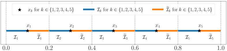
Figure 3: An illustration of ${\mathcal{I}}_{k}$ and ${\widetilde{\mathcal{I}}}_{k}$ for $k\in\{1,2,\mathinner{\mkern-0.1mu\cdotp\mkern-0.3mu\cdotp\mkern-0.3mu\cdotp\mkern-0.1mu},K\}$ with $K=5$.

Our objective is to construct $\phi\in{\hskip 0.6pt\mathcal{N}\mathcal{N}}_{\varrho}\{{\mathcal{O}}(1),\hskip 1.987pt{\mathcal{O}}(1);\hskip 3.0297pt{{\mathbb{R}}}\to{{\mathbb{R}}}\}$ to achieve accurate approximations of $f$ within ${\mathcal{I}}_{k}$ for $k=1,2,\mathinner{\mkern-0.1mu\cdotp\mkern-0.3mu\cdotp\mkern-0.3mu\cdotp\mkern-0.1mu},K$. It is not essential to consider the values of $\phi$ within ${\widetilde{\mathcal{I}}}_{k}$ for all $k$. In other words, our focus is primarily on achieving accurate approximations within one “half” of the interval $[0,1]$, which is the crucial element in our proof.

Define $\psi(x)\coloneqq x-\sigma(x)$ for any $x\in{\mathbb{R}}$, where $\sigma\in{\hskip 0.6pt\mathcal{N}\mathcal{N}}_{\varrho}\{{\mathcal{O}}(1),\hskip 1.987pt{\mathcal{O}}(1);\hskip 3.0297pt{{\mathbb{R}}}\to{{\mathbb{R}}}\}$ with

$$\sigma(x)=\big{|}x-2\big{\lfloor}\tfrac{x+1}{2}\big{\rfloor}\big{|}\quad\textnormal{ for $x\geq 0$.}$$

See Figure 4 for an illustration of $\psi$.

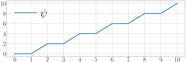
Figure 4: An illustration of $\psi$ on $[0,10]$.

It easy to verifty that

$$\psi(2Kx)/2+1=k\quad\textnormal{for any $x\in[\tfrac{2k-2}{2K},\tfrac{2k-1}{2K}]={\mathcal{I}}_{k}$.}$$ (2)

We will make use of the two following lemmas to simplify our proof.

Lemma 2 (Lemma 23 of Shen et al. (2022)).

Given any rationally independent numbers $a_{1},a_{2},\mathinner{\mkern-0.1mu\cdotp\mkern-0.3mu\cdotp\mkern-0.3mu\cdotp\mkern-0.1mu},a_{K}$ for any $K\in{\mathbb{N}}^{+}$ and an arbitrary periodic function $g:{\mathbb{R}}\to{\mathbb{R}}$ with period $T$, i.e., $g(x+T)=g(x)$ for any $x\in{\mathbb{R}}$, assume there exist $x_{1},x_{2}\in{\mathbb{R}}$ with $0<x_{2}-x_{1}<T$ such that $g$ is continuous on $[x_{1},x_{2}]$. Then the following set

$$\Big{\{}\Big{(}u\cdot g(wa_{1})+v,\,\mathinner{\mkern-0.1mu\cdotp\mkern-0.3mu\cdotp\mkern-0.3mu\cdotp\mkern-0.1mu},\,u\cdot g(wa_{K})+v\Big{)}:u,w,v\in{\mathbb{R}}\Big{\}}$$

is dense in ${\mathbb{R}}^{K}$ provided that

$$\min\limits_{x\in[x_{1},x_{2}]}g(x)<\max\limits_{x\in[x_{1},x_{2}]}g(x)$$.

Lemma 3.

Given $K\in{\mathbb{N}}+$, suppose $\varrho$ is real analytic and non-polynomial on an interval $(\alpha,\beta)$ with $\beta>\alpha$. Then there exists $w_{0}\in\big{(}-\tfrac{\beta-\alpha}{2K},\tfrac{\beta-\alpha}{2K}\big{)}$ such that $\varrho\big{(}\frac{\alpha+\beta}{2}+kw_{0}\big{)}$, for $\{k=1,2,\mathinner{\mkern-0.1mu\cdotp\mkern-0.3mu\cdotp\mkern-0.3mu\cdotp\mkern-0.1mu},K\}$, are rationally independent.

Proof.

We prove this lemma by contradiction. If it does not hold, then $\varrho\big{(}\frac{\alpha+\beta}{2}+kw\big{)}$, for $\{k=1,2,\mathinner{\mkern-0.1mu\cdotp\mkern-0.3mu\cdotp\mkern-0.3mu\cdotp\mkern-0.1mu},K\}$, are rationally dependent for any $w\in\big{(}-\tfrac{\beta-\alpha}{2K},\tfrac{\beta-\alpha}{2K}\big{)}={\mathcal{I}}$. That means, for any $w\in{\mathcal{I}}$, there exists ${\bm{\lambda}}=(\lambda_{1},\mathinner{\mkern-0.1mu\cdotp\mkern-0.3mu\cdotp\mkern-0.3mu\cdotp\mkern-0.1mu},\lambda_{K})\in{\mathbb{Q}}^{K}\backslash\{{\bm{0}}\}$ such that $\sum_{k=1}^{K}\lambda_{k}\varrho\big{(}\frac{\alpha+\beta}{2}+kw\big{)}=0$. We observe that ${\mathcal{I}}$ is uncountable and ${\mathbb{Q}}^{K}\backslash\{{\bm{0}}\}$ is countable. It follows that there exists ${\bm{\lambda}}=(\lambda_{1},\mathinner{\mkern-0.1mu\cdotp\mkern-0.3mu\cdotp\mkern-0.3mu\cdotp\mkern-0.1mu},\lambda_{K})\in{\mathbb{Q}}^{K}\backslash\{{\bm{0}}\}$ such that $\sum_{k=1}^{K}\lambda_{k}\varrho\big{(}\frac{\alpha+\beta}{2}+kw\big{)}=0$ for all $w$ in an uncountable subset of ${\mathcal{I}}$. Then the real analyticity of $\varrho$ implies $\sum_{k=1}^{K}\lambda_{k}\varrho\big{(}\frac{\alpha+\beta}{2}+kw\big{)}=0$ for all $w\in{\mathcal{I}}$. By expanding $\sum_{k=1}^{K}\lambda_{k}\varrho\big{(}\frac{\alpha+\beta}{2}+kw\big{)}$ into the Taylor series at $w=0$, we get the identity $\sum_{k=1}^{K}\lambda_{k}k^{m}=0$ for each $m$ with $\frac{d^{m}\varrho}{dw^{m}}\left(\frac{\alpha+\beta}{2}\right)\neq 0$. Since $\varrho$ is non-polynomial on $(\alpha,\beta)\ni\tfrac{\alpha+\beta}{2}$, there are infinitely many $m$ with $\frac{d^{m}\varrho}{dw^{m}}\left(\frac{\alpha+\beta}{2}\right)\neq 0$, implying $\sum_{k=1}^{K}\lambda_{k}k^{m}=0$. This means ${\bm{\lambda}}=(\lambda_{1},\mathinner{\mkern-0.1mu\cdotp\mkern-0.3mu\cdotp\mkern-0.3mu\cdotp\mkern-0.1mu},\lambda_{K})={\bm{0}}$, a contradiction with ${\bm{\lambda}}\in{\mathbb{Q}}^{K}\backslash\{{\bm{0}}\}$. So we finish the proof of Lemma 3. ∎

Now, let us return to the proof of Theorem 2. We can employ Lemma 3 to produce a collection of rationally independent numbers. Specifically, there exists a value $w_{0}$ such that $a_{1},a_{2},\mathinner{\mkern-0.1mu\cdotp\mkern-0.3mu\cdotp\mkern-0.3mu\cdotp\mkern-0.1mu},a_{K}$ are linearly independent, where each $a_{k}$ is defined as $a_{k}=\varrho\left(\tfrac{\alpha+\beta}{2}+kw_{0}\right)$.

Next, define

$$g(x)=\big{|}x-2\big{\lfloor}\tfrac{x+1}{2}\big{\rfloor}\big{|}\quad\textnormal{ for $x\in{\mathbb{R}}$.}$$

By Lemma 2, there exists $u_{1},w_{1},v_{1}\in{\mathbb{R}}$ such that

$$\big{|}u_{1}\cdot g(w_{1}a_{k})+v_{1}-f(x_{k})\big{|}<\varepsilon/2\quad\textnormal{for any $k$.}$$

Since $\sigma(x)=g(x)$ for any $x\geq 0$ and $g$ is periodic with period $2$, we can choose a sufficiently large $m_{0}\in\mathcal{N}$ such that

$$\begin{split}&\phantom{=\;\;}\big{|}u_{1}\sigma(w_{1}a_{k}+2m_{0})+v_{1}-f(x_{k})\big{|}\\ &=\big{|}u_{1}g(w_{1}a_{k}+2m_{0})+v_{1}-f(x_{k})\big{|}\\ &=\big{|}u_{1}g(w_{1}a_{k})+v_{1}-f(x_{k})\big{|}<\varepsilon/2,\end{split}$$

for $k=1,2,\mathinner{\mkern-0.1mu\cdotp\mkern-0.3mu\cdotp\mkern-0.3mu\cdotp\mkern-0.1mu},K$. Define

$$\phi(x)=u_{1}\sigma\bigg{(}w_{1}\varrho\Big{(}\tfrac{\alpha+\beta}{2}+(\tfrac{\psi(2kx)}{2}-1)w_{0}\Big{)}+2m_{0}\bigg{)}+v_{1}.$$

For any $x\in{\mathcal{I}}_{k}$, we have

$$\begin{split}\phi(x)&=u_{1}\sigma\bigg{(}w_{1}\varrho\Big{(}\tfrac{\alpha+\beta}{2}+(\tfrac{\psi(2kx)}{2}-1)w_{0}\Big{)}+2m_{0}\bigg{)}+v_{1}\\ &=u_{1}\sigma\Big{(}w_{1}\varrho\big{(}\tfrac{\alpha+\beta}{2}+kw_{0}\big{)}+2m_{0}\Big{)}+v_{1}\\ &=u_{1}\sigma\Big{(}w_{1}a_{k}+2m_{0}\Big{)}+v_{1},\end{split}$$

implying

$$|\phi(x)-f(x)|\leq\underbrace{|\phi(x)-f(x_{k})|}_{<\varepsilon/2}+\underbrace{|f(x_{k})-f(x)|}_{<\varepsilon/2\textnormal{ by }\eqref{eq:f:error:1/K}}<\varepsilon.$$

It follows that

$$|\phi(x)-f(x)|<\varepsilon\quad\textnormal{for any}\ x\in\bigcup_{k=0}^{K-1}\big{[}\tfrac{2k}{2K},\tfrac{2k+1}{2K}\big{]}.$$

Moreover, we can easily verify $\phi\in{\hskip 0.6pt\mathcal{N}\mathcal{N}}_{\varrho}\{{\mathcal{O}}(1),\hskip 1.987pt{\mathcal{O}}(1);\hskip 3.0297pt{{\mathbb{R}}}\to{{\mathbb{R}}}\}$. So we finish the proof of Theorem 2.

3.2 Proof of Theorem 3 based on Theorem 2.

We claim it suffices to prove the special case $[a,b]=[0,\tfrac{1}{2}]$ as this simplification readily extends to the broader scenario. To see this, we simply introduce a linear function ${\mathcal{L}}:[0,\tfrac{1}{2}]\to[a,b]$ by defining ${\mathcal{L}}(x)=2(b-a)x+a$. The special case implies $f\circ{\mathcal{L}}:[0,\tfrac{1}{2}]\to{\mathbb{R}}$ can be approximated by a network ${\widetilde{\phi}}$ arbitrarily well. Then $\phi={\widetilde{\phi}}\circ{\mathcal{L}}^{-1}$ can approximate $f:[a,b]\to{\mathbb{R}}$ well, as desired.

We can continuously extend $f$ from $[0,\tfrac{1}{2}]$ to ${\mathbb{R}}$ by setting $f(x)=f(0)$ if $x<0$ and $f(x)=f(\tfrac{1}{2})$ if $x>\frac{1}{2}$. It follows from the uniform continuity of $f$ on $[-1,2]$ that there exists $K=K(f,\varepsilon)\in{\mathbb{N}}^{+}$ with $K\geq 2$ such that for any $x_{1},x_{2}\in[-1,2]$,

$$|f(x_{1})-f(x_{2})|<\varepsilon/10\quad\textnormal{if $|x_{1}-x_{2}|<1/K$.}$$

For $i=1,2,3,4$, define

$$f_{i}(x)\coloneqq f\big{(}x-\tfrac{i}{4K}\big{)}\quad\textnormal{for any $x\in[0,1]$.}$$

Then, for $i=1,2,3,4$ and $x_{1},x_{2}\in[0,1]$, we have

$$|f_{i}(x_{1})-f_{i}(x_{2})|<\varepsilon/10={\widetilde{\varepsilon}}/2\quad\textnormal{if $|x_{1}-x_{2}|<1/K$,}$$

where ${\widetilde{\varepsilon}}=\varepsilon/5$. For each $i\in\{1,2,3,4\}$, by Theorem 2, there exists $\phi_{i}\in{\hskip 0.6pt\mathcal{N}\mathcal{N}}_{\varrho}\{{\mathcal{O}}(1),\hskip 1.987pt{\mathcal{O}}(1);\hskip 3.0297pt{{\mathbb{R}}}\to{{\mathbb{R}}}\}$ such that

$$\big{|}\phi_{i}(x)-f_{i}(x)\big{|}<\widetilde{\varepsilon}=\varepsilon/5\quad\textnormal{for any}\ x\in\bigcup_{k=0}^{K-1}\big{[}\tfrac{2k}{2K},\tfrac{2k+1}{2K}\big{]}.$$

Define

$$\psi(x)=\sigma\big{(}x+1-\sigma(x+1)\big{)}\quad\textnormal{for any $x\in{\mathbb{R}}$,}$$

where $\sigma\in{\hskip 0.6pt\mathcal{N}\mathcal{N}}_{\varrho}\{{\mathcal{O}}(1),\hskip 1.987pt{\mathcal{O}}(1);\hskip 3.0297pt{{\mathbb{R}}}\to{{\mathbb{R}}}\}$ with

$$\sigma(x)=\big{|}x-2\big{\lfloor}\tfrac{x+1}{2}\big{\rfloor}\big{|}\quad\textnormal{ for $x\geq 0$.}$$

See an illustration of $\psi$ on $[0,2K]$ for $K=5$ in Figure 5.

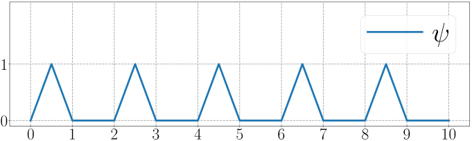
Figure 5: An illustration of $\psi$ on $[0,2K]$ for $K=5$.

Clearly, $0\leq\psi(2Kx)\leq 1$ for any $x\in[0,1]$, from which we deduce

$$\Big{|}\big{(}\phi_{i}(x)-f_{i}(x)\big{)}\psi(2Kx)\Big{|}<\varepsilon/5\quad{\forall\,}\ x\in\bigcup_{k=0}^{K-1}\big{[}\tfrac{2k}{2K},\tfrac{2k+1}{2K}\big{]}.$$

Observe that $\psi(y)=0$ for $y\in\bigcup_{k=0}^{K-1}[{2k+1},{2k+2}]$, which implies

$$\psi(2Kx)=0\quad\textnormal{for any $x\in\bigcup_{k=0}^{K-1}[\tfrac{2k+1}{2K},\tfrac{2k+2}{2K}]$}.$$

Subsequently, by the fact

$$[0,1]=\Bigg{(}\bigcup_{k=0}^{K-1}\big{[}\tfrac{2k}{2K},\tfrac{2k+1}{2K}\big{]}\Bigg{)}\bigcup\Bigg{(}\bigcup_{k=0}^{K-1}\big{[}\tfrac{2k}{2K},\tfrac{2k+1}{2K}\big{]}\Bigg{)},$$

we have

$$\Big{|}\big{(}\phi_{i}(x)-f_{i}(x)\big{)}\psi(2Kx)\Big{|}<\varepsilon/5\quad\textnormal{for any $x\in[0,1]$}.$$ (3)

For each $i\in\{1,2,3,4\}$ and any $z\in[0,\tfrac{1}{2}]\subseteq[0,1-\tfrac{1}{K}]\subseteq[0,1-\tfrac{i}{4K}]$, we have

$$y_{i}=z+\tfrac{i}{4K}\in[\tfrac{i}{4K},1]\subseteq[0,1].$$

By bringing $x=y_{i}\in[0,1]$ into Equation (3), we get

$$\begin{split}&\phantom{=\;\;}\varepsilon/5>\Big{|}\big{(}\phi_{i}(y_{i})-f_{i}(y_{i})\big{)}\psi(2Ky_{i})\Big{|}\\ &=\Big{|}\phi_{i}(y_{i})\psi(2Ky_{i})-f_{i}(y_{i})\psi(2Ky_{i})\Big{|}\\ &=\Big{|}\phi_{i}(z+\tfrac{i}{4K})\psi\big{(}2K(z+\tfrac{i}{4K})\big{)}-f_{i}(z+\tfrac{i}{4K})\psi\big{(}2K(z+\tfrac{i}{4K})\big{)}\Big{|}\\ &=\Big{|}\phi_{i}(z+\tfrac{i}{4K})\psi\big{(}2Kz+\tfrac{i}{2}\big{)}-f(z)\psi\big{(}2Kz+\tfrac{i}{2}\big{)}\Big{|}\end{split}$$

for any $z\in[0,\tfrac{1}{2}]$, where the last equality comes from the fact that $f_{i}(x)=f(x-\tfrac{i}{4K})$ for any $x\in[0,1]\supseteq[\tfrac{i}{4K},1]$. Define

$${\widetilde{\phi}}(x)\coloneqq\sum_{i=1}^{4}\phi_{i}(x+\tfrac{i}{4K})\psi\big{(}2Kx+\tfrac{i}{2}\big{)}\quad\textnormal{for any $x\in[0,\tfrac{1}{2}]$.}$$

It is easy to verify that $\sum_{i=1}^{4}\psi\big{(}x+\tfrac{i}{2}\big{)}=1$ for any $x\geq 0$ based on the definition of $\psi$. See Figure 6 for illustrations. It follows that $\sum_{i=1}^{4}\psi\big{(}2Kz+\tfrac{i}{2}\big{)}=1$ for any $z\in[0,\tfrac{1}{2}]$.

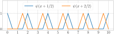
(a)

(b)

(c)

(d)

Figure 6: Illustrations of $\sum_{i=1}^{4}\psi(x+i/2)=1$ for any $x\in[0,10]$.

Hence, for any $z\in[0,\tfrac{1}{2}]$, we have

$$\begin{split}&\quad\;\big{|}{\widetilde{\phi}}(z)-f(z)\big{|}\\ &=\Big{|}\sum_{i=1}^{4}\phi_{i}(z+\tfrac{i}{4K})\psi\big{(}2Kz+\tfrac{i}{2}\big{)}-f(z)\sum_{i=1}^{4}\psi\big{(}2Kz+\tfrac{i}{2}\big{)}\Big{|}\\ &\leq\sum_{i=1}^{4}\Big{|}\phi_{i}(z+\tfrac{i}{4K})\psi\big{(}2Kz+\tfrac{i}{2}\big{)}-f(z)\psi\big{(}2Kz+\tfrac{i}{2}\big{)}\Big{|}\\ &<4\cdot\frac{\varepsilon}{5}=\frac{4\varepsilon}{5}.\end{split}$$

To approximate $(x,y)\mapsto xy$ well, we define

$$\Gamma_{\delta}(x,y)\coloneqq\tfrac{\varrho(x_{0}+\delta x+\delta y)-\varrho(x_{0}+\delta y)-\varrho(x_{0}+\delta x)+\varrho(x_{0})}{\delta^{2}\varrho^{\prime\prime}(x_{0})}$$

for any $x,y\in{\mathbb{R}}$, where $\varrho^{\prime\prime}(x_{0})\neq 0$. Clearly, $\Gamma_{\delta}(x,y)\to xy$ as $\delta\to 0$. Then we can define

$$\phi_{\delta}(x)\coloneqq\sum_{i=1}^{4}\Gamma_{\delta}\Big{(}\phi_{i}(x+\tfrac{i}{4K}),\,\psi\big{(}2Kx+\tfrac{i}{2}\big{)}\Big{)}\quad\textnormal{ ${\forall\,}x\in[0,\tfrac{1}{2}]$.}$$

Clearly, $\phi_{\delta}\in{\hskip 0.6pt\mathcal{N}\mathcal{N}}_{\varrho}\{{\mathcal{O}}(1),\hskip 1.987pt{\mathcal{O}}(1);\hskip 3.0297pt{{\mathbb{R}}}\to{{\mathbb{R}}}\}$. Moreover, we can choose a sufficiently small $\delta_{0}>0$ such that

$$|\phi_{\delta_{0}}(x)-{\widetilde{\phi}}(x)|<\varepsilon/5\quad\textnormal{for any $x\in[0,\tfrac{1}{2}]$.}$$

By defining $\phi\coloneqq\phi_{\delta_{0}}\in{\hskip 0.6pt\mathcal{N}\mathcal{N}}_{\varrho}\{{\mathcal{O}}(1),\hskip 1.987pt{\mathcal{O}}(1);\hskip 3.0297pt{{\mathbb{R}}}\to{{\mathbb{R}}}\}$, we have

$$\begin{split}|\phi(x)-f(x)|\leq\underbrace{|\phi_{\delta_{0}}(x)-{\widetilde{\phi}}(x)|}_{<\varepsilon/5}+\underbrace{|{\widetilde{\phi}}(x)-f(x)|}_{<4\varepsilon/5}<\varepsilon\end{split}$$

for any $x\in[0,\tfrac{1}{2}]$. So we finish the proof of Theorem 3.

Table 1: A Brief Description of Three Image Datasets and Four Industrial Fault Diagnosis Datasets

Dataset	Description
CIFAR-10	60,000 32×32 resolution RGB images in 10 categories (6,000 images per category)
Tiny ImageNet	100,000 64×64 RGB images in 200 categories (500 for each category)
ImageNet	14,197,122 RGB images over 1,000 categories and 21,841 subcategories
Case Western Reserve University (CWRU )	2,400 vibration signals with 10 types of faults in drive end. Each signals has 1,024 samples
Power Quality Disturbance (PQD)	11200 voltage disturbance signals in 16 types, each disturbance signal at each fault has additive white Gaussian noise
Motor Fault (MF)	6 types of faults and each kind of fault has at least 290 samples  (Sun et al., 2023)
Electrical Fault Detection and Classification (EFDC)	12,000 samples with 6 types of faults. Each sample has 6 features including the measured line currents and voltages.

3.3 Proof of Theorem 1 based on Theorem 3 and KST.

We can safely assume that $[a,b]=[0,1]$ since the general case can be readily extended by incorporating an affine map such as ${\mathcal{L}}(a)=(b-a)x+a$. Given any $f\in C([0,1]^{d})$, by KST, there exist $h_{i,j}\in C([0,1])$ and $g_{i}\in C({\mathbb{R}})$ for $i=0,1,\mathinner{\mkern-0.1mu\cdotp\mkern-0.3mu\cdotp\mkern-0.3mu\cdotp\mkern-0.1mu},2d$ and $j=1,2,\mathinner{\mkern-0.1mu\cdotp\mkern-0.3mu\cdotp\mkern-0.3mu\cdotp\mkern-0.1mu},d$ such that

$$f({\bm{x}})=\sum_{i=0}^{2d}g_{i}\Big{(}\sum_{j=1}^{d}h_{i,j}(x_{j})\Big{)}\quad{\forall\,}\textnormal{ ${\bm{x}}=(x_{1},\mathinner{\mkern-0.1mu\cdotp\mkern-0.3mu\cdotp\mkern-0.3mu\cdotp\mkern-0.1mu},x_{d})\in[0,1]^{d}$.}$$

Choose a sufficiently large $A>0$, e.g.,

$$A=1+\sup\bigg{\{}\Big{|}\sum_{j=1}^{d}h_{i,j}(x_{j})\Big{|}:i=0,1,\mathinner{\mkern-0.1mu\cdotp\mkern-0.3mu\cdotp\mkern-0.3mu\cdotp\mkern-0.1mu},2d,\;\ {\bm{x}}\in[0,1]^{d}\bigg{\}}.$$

Then for any $\delta>0$, by Theorem 3, there exist $\psi_{i,j},\phi_{i}\in{\hskip 0.6pt\mathcal{N}\mathcal{N}}_{\varrho}\{{\mathcal{O}}(1),\hskip 1.987pt{\mathcal{O}}(1);\hskip 3.0297pt{{\mathbb{R}}}\to{{\mathbb{R}}}\}$ such that

$$|g_{i}(t)-\phi_{i}(t)|<\delta\quad\textnormal{for any $t\in[-A,A]$}$$

and

$$|h_{i,j}(t)-\psi_{i,j}(t)|<\delta\quad\textnormal{for any $t\in[0,1]$,}$$

for $i=0,1,\mathinner{\mkern-0.1mu\cdotp\mkern-0.3mu\cdotp\mkern-0.3mu\cdotp\mkern-0.1mu},2d$ and $j=1,2,\mathinner{\mkern-0.1mu\cdotp\mkern-0.3mu\cdotp\mkern-0.3mu\cdotp\mkern-0.1mu},d$. By defining

$$\phi({\bm{x}})=\sum_{i=0}^{2d}\phi_{i}\Big{(}\sum_{j=1}^{d}\psi_{i,j}(x_{j})\Big{)}\quad{\forall\,}\textnormal{ ${\bm{x}}=(x_{1},\mathinner{\mkern-0.1mu\cdotp\mkern-0.3mu\cdotp\mkern-0.3mu\cdotp\mkern-0.1mu},x_{d})\in{\mathbb{R}}^{d}$.}$$

we have $\phi\in{\hskip 0.6pt\mathcal{N}\mathcal{N}}_{\varrho}\{{\mathcal{O}}(d^{2}),\hskip 1.987pt{\mathcal{O}}(1);\hskip 3.0297pt{{\mathbb{R}}}\to{{\mathbb{R}}}\}$. See an illustration of the architecture of $\phi$ in Figure 7. Moreover, by choosing sufficiently small $\delta>0$, we can conclude that

$$|\phi({\bm{x}})-f({\bm{x}})|<\varepsilon\quad{\forall\,}{\bm{x}}\in[0,1]^{d},$$

which means we finish the proof of Theorem 1.

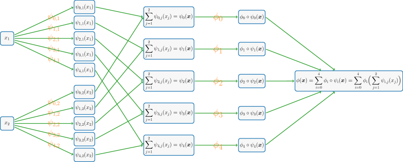
Figure 7: An illustration of the target network realizing $\phi$ for any ${\bm{x}}\in[a,b]^{d}$ in the case of $d=2$. This network contains $(2d+1)d+(2d+1)=(d+1)(2d+1)$ sub-networks that realize $\psi_{i,j}$ and $\phi_{i}$ for $i=0,1,\mathinner{\mkern-0.1mu\cdotp\mkern-0.3mu\cdotp\mkern-0.3mu\cdotp\mkern-0.1mu},2d$ and $j=1,2,\mathinner{\mkern-0.1mu\cdotp\mkern-0.3mu\cdotp\mkern-0.3mu\cdotp\mkern-0.1mu},d$.

4 Experimental Results

To further validate the efficacy of our activation functions, we evaluate PEUAF against a wide range of baseline activation functions, including LReLU (Xu et al., 2015), PReLU (He et al., 2015), Softplus (Zheng et al., 2015), ELU (Clevert et al., 2015), SELU (Klambauer et al., 2017), ReLU (Nair and Hinton, 2010) and Swish (Ramachandran et al., 2017). We conduct these comparisons across four industrial signal datasets and three image datasets (CIFAR-10  (Krizhevsky et al., 2009), Fashion-MNIST (Xiao et al., 2017) and ImageNet (Deng et al., 2009)) using three distinct neural network architectures (LeNet-type (Lecun et al., 1998), ResNet-18  (He et al., 2016), and VGG-16  (Simonyan and Zisserman, 2015)).

As discussed in (Shen et al., 2022), only a few neurons with super-expressive activation functions are required to approximate functions with arbitrary precision to avoid large generalization errors. However, implementing this in practical experiments is challenging. Therefore, our experiments primarily focus on exploring the feature patterns of PEUAF and determining how it contributes to improving test accuracy, instead of targeting 100% test accuracy.

4.1 Experimental Setups

The datasets used in our experiments are briefly introduced in Table 1. For each experiment, we train the models with a batch size of 64 using the “NAdam” optimizer  (Dozat, 2016), with an initial learning rate of $0.01$. The learning rate decays with a factor of 0.2 if the accuracy change over 5 consecutive epochs is no more than $1\times 10^{-4}$. We set the number of epochs to 300 to ensure proper convergence. The baseline network structures employed in our experiments are introduced in Tables 2 and 3.

Table 2: Baseline A for the CWRU, PQD, and MF datasets.

Layer	Parameters	Activation
1D-Convolution $(3\times 1)$	filter size=64, stride = 1	PEUAF
1D-Convolution $(3\times 1)$	filter size=64, stride = 1	PEUAF
Batch-normalization (BN)	momentum=0.99, epsilon=0.001	–
Max-pooling	pool size=$3\times 1$, stride = 1	–
1D-Convolution $(3\times 1)$	filter size=64, stride = 1	PEUAF
1D-Convolution $(3\times 1)$	filter size=64, stride = 1	PEUAF
Batch-normalization (BN)	momentum=0.99, epsilon=0.001	–
Max-pooling	pool size=$3\times 1$, stride = 1	–
1D-Convolution $(3\times 1)$	filter size=64, stride = 1	PEUAF
1D-Convolution $(3\times 1)$	filter size=64, stride = 1	PEUAF
Batch-normalization (BN)	momentum=0.99, epsilon=0.001	–
Global-average-pooling	–	–
Fully connected	size (chosen by tasks)	softmax

Table 3: Baseline B for the EFDC dataset.

Layer	Parameters	Activation
1D-Convolution $(2\times 1)$	filter size=16, stride = 1	PEUAF
Batch-normalization (BN)	momentum=0.99, epsilon=0.001	–
Max-pooling	pool size=$2\times 1$, stride = 1	–
1D-Convolution $(2\times 1)$	filter size=16, stride = 1	PEUAF
Batch-normalization (BN)	momentum=0.99, epsilon=0.001	–
Max-pooling	pool size=$2\times 1$, stride = 1	–
Flatten	–	–
Fully connected	size (chosen by tasks)	softmax

The most critical hyperparameter is the range of the adaptive frequency $w$. To determine this, we conducted a classification experiment with different $w$ values on the PQD dataset  (A et al., ), as illustrated in Figure 8. The network structure used is Baseline A, a 1D convolutional neural network. To emphasize the discrepancies in outcomes, we employ a logarithmic transformation ($\log$) during the visualization of the loss function. Figure 8 shows the training and validation curves, while Table 4 provides the corresponding test accuracy. The table reveals two key points: First, when $w$ exceeds 1, the test accuracy drops significantly, indicating that higher frequencies pose challenges to the PEUAF’s ability to effectively extract PQD features. Second, when $w$ lies in the range of $[0,1]$, the test accuracy consistently remains above 98%. Therefore, we reasonably conclude that the frequency $w$ should be constrained within the range of $[0,1]$.

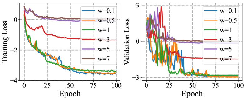
Figure 8: The training and validation loss with different $w$. (a) the training loss; (b) the validation loss

Table 4: The accuracy of PQD classification with different $w$.

$w$	0.1	0.5	1	3	5	7
Accuracy	98.25$\%$	98.30$\%$	98.04$\%$	93.66$\%$	75.26$\%$	53.39$\%$

4.2 Analysis Experiments

In this section, we conduct experiments to show the characteristics of PEUAF. For the larger datasets (CWRU, PQD, and MF), we utilize the Baseline A in Table 2, while for the EFDC dataset, we use the Baseline B in Table 3. Baseline B is smaller than Baseline A due to the smaller size of the EFDC dataset compared to CWRU, PQD, and MF. Our comparison focuses not only on the overall performance but also on the convergence behavior during the training process, fluctuations in the validation process, and a detailed mechanism analysis.

Table 5: Test accuracy in industrial fault diagnosis datasets.

Model	CWRU	PQD	MF	EFDC	Avg Rank
LReLU	99.58$\%$	98.12$\%$	98.82$\%$	84.24$\%$	4
PReLU	97.08$\%$	97.85$\%$	99.17$\%$	84.50$\%$	7
Softplus	95.00$\%$	97.95$\%$	98.06$\%$	84.37$\%$	8
ELU	100.00$\%$	98.15$\%$	99.70$\%$	83.10$\%$	2
SELU	99.17$\%$	98.12$\%$	99.85$\%$	83.74$\%$	3
ReLU	99.58$\%$	97.89$\%$	99.70$\%$	83.35$\%$	5
Swish	99.16$\%$	98.15$\%$	97.35$\%$	84.63$\%$	6
PEUAF	100.00$\%$	98.17$\%$	100.00$\%$	85.64$\%$	1

Performance. Table 5 summarizes the performance of several activation functions. All results are the average over three runs. On the EFDC dataset, PEUAF takes the lead by the largest margin, i.e., surpassing the second place Swish by over $1\%$. On the CWRU, dataset, PEUAF exhibits competitive performance compared to Swish, ReLU, SELU, ELU, and LReLU, while PEUAF outperforms Softplus and PReLU by 2% and 5%, respectively. On the PQD dataset, all activation functions achieve similar test accuracy. Lastly, on the MF dataset, PEUAF shows similar performance with ReLU, SELU, ELU, and PReLU but surpasses Swish and Softplus. Overall, PEUAF proves to be a competent activation function on four industrial fault diagnosis datasets.

To further evaluate the effectiveness of PEUAF, we conducted occlusion experiments in two classic datasets: CWRU and PQD. For each dataset, the occluding sizes and strides were set to 100 and 50, respectively. The occluded pixels were all replaced by zeros. Based on the results in Figure 9, we observe that PEUAF outperforms ReLU in locating faults. The experiments reveal two distinct levels of performances: (1) In the PQD dataset, PEUAF and ReLU show similar performance in accurately detecting and localizing faults, as illustrated in Figure 9. This can be attributed to the favorable condition within the PQD dataset, characterized by its low signal-to-noise ratio, contributing to the successful faults localization. However, such ideal conditions are rare in real-world scenarios. (2) In contrast, in the CWRU dataset, PEUAF significantly outperforms ReLU as shown in Figure 9. Despite that both PEUAF and ReLU achieve commendable test accuracy, ReLU tends to capture more holistic features instead of locating the real fault, which makes the outputs less reliable. Conversely, PEUAF effectively locates faults even in the presence of noise interference, offering valuable insights into the timing and severity of fault occurrences, as indicated by the occlusion experiments.

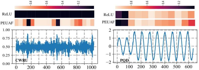
Figure 9: Occlusion experiments of Baselines using PEUAF and ReLU in CWRU and PQD datasets. It is seen that the baseline with PEUAF can better localize the fault when the original signal is noisy.

Convergence. Since PEUAF has a unique shape, there might be concerns that such an oscillating function could be difficult to optimize. To address this, we compare the training dynamics of PEUAF and ReLU. Figure 10 shows the training and validation curves of PEUAF and ReLU on the CWRU, PQD, and MF datasets. Below are our detailed analyses:

1. Convergence speed during training: The convergence rate during the training process is notably influenced by the choice of activation functions and the inherent characteristics of the dataset. All the experiments in Figure 10 consistently demonstrate the superior convergence speed of PEUAF. In dataset with a lower signal-to-noise ratio (such as the PQD dataset), PEUAF and ReLU show similar convergence speed. In contrast, in noise-free datasets or those with high signal-to-noise ratio, models adopting the PEUAF activation function display significantly faster convergence.

2. Convergence effect during training: The choice of activation functions can impact the convergence effect, particularly in terms of oscillations or fluctuations during the training process. In the PQD dataset, the convergence patterns of PEUAF and ReLU are relatively similar, except for some fluctuations occurring around the 50th epoch. However, for the MF dataset, noticeable oscillations occur during convergence, particularly within the epoch range between 150 to 200. For the CWRU dataset, the fluctuations happen at around the 50th epoch when using ReLU as the activation function. Therefore, PEUAF helps reduce the oscillation of training losses and improves the training performance.

3. Fluctuation during validation: In addition to the training process, the effectiveness of PEUAF can also be observed during the validation process. Across all the datasets, PEUAF outperforms ReLU by showing less fluctuation in the validation process. For the CWRU dataset, both PEUAF and ReLU exhibit fluctuations at the start of the validation process. However, after a sudden drop in validation loss after approximately 20 epochs, PEUAF shows smaller validation loss fluctuations than ReLU. For the PQD dataset, the validation loss curve for PEUAF and ReLU appear similar, but the amplitude of fluctuations is smaller for PEUAF. The most significant difference in fluctuation patterns is particularly obvious in the MF dataset, where ReLU exhibits high frequency and amplitude of fluctuations. This behavior can potentially be attributed to the fact that, in noise-free data settings, ReLU tends to capture global features initially, rather than precisely pinpointing fine-grained fault details, unlike PEUAF.

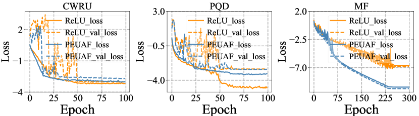
Figure 10: Training dynamics of Baselines using PEUAF and ReLU in three large datasets.

4.3 Comparative Experiments

In this section, we demonstrate combining the super-expressive activation function (PEUAF) with the baseline activation function can enhance the generalization ability of neural networks.

CIFAR-10. In this experiment, we augment the dataset by rotating, shifting, shearing, and horizontally flipping the original images. We mainly focus on the ResNet structure. Table 6 compares ResNet-18a with a mixed activation function to several identical model topologies using ReLU. The mixed activation function achieves a 0.89$\%$ error reduction. Tables 7 and  8 separately summarize the test accuracy of ResNet-18 and Vit-B/16 (Dosovitskiy et al., 2020) across various baseline activation functions and mixed activation functions. Notably, the mixed activation function improves the test accuracy, especially in Softplus, which increased by 2.72$\%$ and 5.01$\%$.

Table 6: CIFAR-10 Classifcation error vs the number of parameters, for common compact model architectures vs. ResNet-18a + Mixed ReLU.

Neural Network	$\#$Param	Error$\%$
All-CNN (Springenberg et al., 2014)	1.3M	7.25$\%$
MobileNetV1 (Howard et al., 2017)	3.2M	10.76$\%$
MobileNetV2 (Sandler et al., 2018)	2.24M	7.22$\%$
ShuffleNet 8G (Zhang et al., 2018)	0.91M	7.71$\%$
ShuffleNet 1G (Zhang et al., 2018)	0.24M	8.56$\%$
HENet (Duan et al., 2018)	0.7M	10.16$\%$
ResNet-18a+ReLU	0.27M	8.75$\%$
ResNet-18a+ mixed ReLU	0.27M	7.82$\%$

To further explain the efficacy of mixed activation functions, Figure 11 provides a detailed comparison of the loss and accuracy among ReLU, PEUAF and mixed activation functions. When exclusively applying PEUAF in the CIFAR-10 classification task, both the training convergence and fluctuations are worse than those of ReLU, as shown in the loss curve in Figure 11. However, the ResNet-18 using mixed activation functions outperforms the models using either ReLU or PEUAF alone. The mixed approach results in smoother loss and accuracy curves during both the training and validation process.

The occlusion experiments further demonstrate that the mixed activation functions can enhance the neural network’s ability to identify essential features. The occlusion sizes and strides are set to 4 and 2, respectively, with occluded pixels replaced by zeros. As in Figure LABEL:fig:Occlusion_experiments_of_2D_convolution_experiments, the results provide a clear illustration of this phenomenon. The models using only ReLU or PEUAF successfully identify a multitude of features contributing to the classification. However, they also select too many unnecessary pixel points, recognizing part of the surroundings as the important features for classification. In contrast, the mixed activation function model can accurately locate the critical features while ignoring irrelevant pixels.

Table 7: Comparisons of classification accuracy across several activation functions using ResNet for CIFAR-10.

Activation	Test accuracy
ResNet-18+PEUAF	90.00$\%$ / -
ResNet-18+LReLU/Mixed	92.42$\%$ / 94.13$\%$
ResNet-18+PReLU/Mixed	92.29$\%$ / 94.23$\%$
ResNet-18+Softplus/Mixed	89.28$\%$ / 92.09$\%$
ResNet-18+ELU/Mixed	91.09$\%$ / 92.11$\%$
ResNet-18+SELU/Mixed	90.47$\%$ / 91.32$\%$
ResNet-18+ReLU/Mixed	93.02$\%$ / 93.91$\%$
ResNet-18+Swish/Mixed	94.07$\%$ / 92.99$\%$
ResNet-34+ReLU/Mixed	93.70$\%$ / 94.23$\%$

Table 8: Comparisons of classification accuracy across several activation functions using Vit-B/16 for CIFAR-10.

Activation	Test accuracy
Vit-B/16+PEUAF	90.58$\%$ / -
Vit-B/16+LReLU/Mixed	91.15$\%$ / 91.31$\%$
Vit-B/16+PReLU/Mixed	90.40$\%$ / 90.47$\%$
Vit-B/16+Softplus/Mixed	74.23$\%$ / 79.24$\%$
Vit-B/16+ELU/Mixed	89.69$\%$ / 89.80$\%$
Vit-B/16+SELU/Mixed	87.26$\%$ / 87.37$\%$
Vit-B/16+ReLU/Mixed	89.43$\%$ / 89.44$\%$
Vit-B/16+Swish/Mixed	90.66$\%$ / 89.65$\%$
Vit-B/16+GELU/Mixed	97.49$\%$ / 97.90$\%$

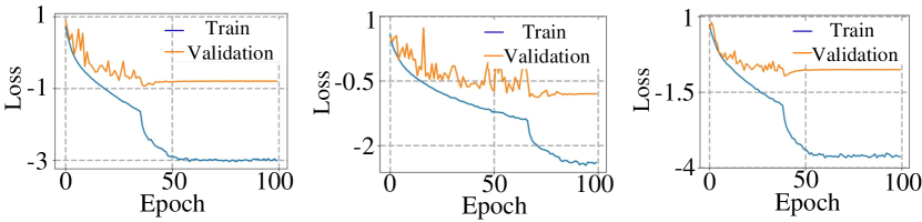
Figure 11: Loss of CIFAR-10 experiments among three activation functions. From left to right are the loss of ResNet-18 using ReLU, PEUAF and mixed activation function.

Tiny-ImageNet. The Tiny-Imagenet dataset is utilized to further demonstrate the expressiveness of PEUAF. The model is trained for 100 epochs with an initial learning rate of 0.1, which decays by an order of magnitude every 30 epochs, using a batch size of 256. Table 9 compares the test accuracy of ResNet-18 with several baseline activation functions on Tiny-ImageNet. By replacing the activation functions in the last block, the ResNet-18 with mixed activation functions achieves competitive results, showing slight improvements in the test accuracy across most experiments, except for Swish and PEUAF.

Table 9: Comparisons of classification accuracy across several activation functions using ResNet-18 for Tiny-ImageNet.

Activation	Test accuracy
ResNet-18+PEUAF	56.86$\%$ / -
ResNet-18+LReLU/Mixed	62.39$\%$ / 62.29$\%$
ResNet-18+PReLU/Mixed	59.57$\%$ / 60.81$\%$
ResNet-18+Softplus/Mixed	56.98$\%$ / 57.75$\%$
ResNet-18+ELU/Mixed	59.44$\%$ / 59.88$\%$
ResNet-18+SELU/Mixed	59.51$\%$ / 59.62$\%$
ResNet-18+ReLU/Mixed	63.40$\%$ / 63.42$\%$
ResNet-18+Swish/Mixed	60.76$\%$ / 59.53$\%$

ImageNet. The ImageNet dataset is used to evaluate the effectiveness of PEUAF in large datasets. Due to memory limitations, the model follows the setup from the previous research (Liu et al., 2022b), except for the number of neurons in the first layer and the data enhancement. The neurons of the first layer is reduced to 256 from 512. Table 10 compares the test accuracy between PReLU and the mixed activation. In this large-scale image classification experiment, the drawbacks of using PEUAF alone become apparent, with the accuracy of ResNet-18 with PEUAF being only 63.38%, which is lower than that of PReLU. However, the ResNet-18 with mixed activation functions achieves competitive results.

Table 10: Comparisons of classification accuracy across several activation functions using ResNet-18 for ImageNet.

Activation	Test accuracy
ResNet-18+PEUAF	63.38$\%$ / -
ResNet-18+LReLU/Mixed	70.65$\%$ / 70.96$\%$

5 Conclusion and Discussion

This paper provides an in-depth analysis of the characteristics and effectiveness of PEUAF, particularly focusing on its application to industrial and image datasets. By testing the trainable frequency $w$, we have determined an optimal frequency range for $w$ within the interval $[0,1]$. To further demonstrate the super-expressiveness of PEUAF, we have conducted experiments using four industrial datasets and three benchmark image datasets. The results indicate that PEUAF surpasses ReLU in terms of convergence speed, oscillation during training, fluctuation during validation, and fault localization ability, especially in industrial datasets with a high signal-to-noise ratio. Additionally, the mixed activation function outperforms the single activation function in most image classification tasks.

Looking ahead, the future of activation function research is promising. The development of PEUAF paves the way for exploring other super-expressive activation functions that could further enhance neural network performance across various applications. Future research could focus on expanding the family of super-expressive activation functions and investigating their practical utility in more diverse and complex datasets. Moreover, combining PEUAF with other state-of-the-art neural network architectures and exploring its benefits in real-world scenarios could yield valuable insights. The adaptability and effectiveness of PEUAF in handling stationary signals suggest potential applications in fields such as signal processing, fault diagnosis, and time-series analysis.

References

- (1) A, R.M., A, A.C., B, J.B., C, Y.B., A, Y.L., . Open source dataset generator for power quality disturbances with deep-learning reference classifiers - sciencedirect. Electric Power Systems Research 195.
- Apicella et al. (2021) Apicella, A., Donnarumma, F., Isgrò, F., Prevete, R., 2021. A survey on modern trainable activation functions. Neural Networks 138, 14–32.
- Bingham and Miikkulainen (2022) Bingham, G., Miikkulainen, R., 2022. Discovering parametric activation functions. Neural Networks 148, 48–65.
- Clevert et al. (2015) Clevert, D.A., Unterthiner, T., Hochreiter, S., 2015. Fast and accurate deep network learning by exponential linear units (ELUs). arXiv preprint arXiv:1511.07289 .
- Deng et al. (2009) Deng, J., Dong, W., Socher, R., Li, L.J., Li, K., Fei-Fei, L., 2009. Imagenet: A large-scale hierarchical image database, in: 2009 IEEE conference on computer vision and pattern recognition, IEEE. pp. 248–255.
- Dosovitskiy et al. (2020) Dosovitskiy, A., Beyer, L., Kolesnikov, A., Weissenborn, D., Zhai, X., Unterthiner, T., Dehghani, M., Minderer, M., Heigold, G., Gelly, S., et al., 2020. An image is worth 16x16 words: Transformers for image recognition at scale. arXiv preprint arXiv:2010.11929 .
- Dozat (2016) Dozat, T., 2016. Incorporating nesterov momentum into adam. ICLR workshop.
- Duan et al. (2018) Duan, J., Zhang, R., Huang, J., Zhu, Q., 2018. The speed improvement by merging batch normalization into previously linear layer in cnn, in: 2018 International Conference on Audio, Language and Image Processing (ICALIP), IEEE. pp. 67–72.
- Fan et al. (2020) Fan, F., Li, M., Teng, Y., Wang, G., 2020. Soft autoencoder and its wavelet adaptation interpretation. IEEE Transactions on Computational Imaging 6, 1245–1257.
- Gao and Zhang (2023) Gao, F., Zhang, B., 2023. Data-aware customization of activation functions reduces neural network error. arXiv preprint arXiv:2301.06635 .
- Goldenstein et al. (2024) Goldenstein, N., Sulam, J., Romano, Y., 2024. Pivotal auto-encoder via self-normalizing relu. IEEE Transactions on Signal Processing , 1–12doi:10.1109/TSP.2024.3418971.
- He et al. (2015) He, K., Zhang, X., Ren, S., Sun, J., 2015. Delving deep into rectifiers: Surpassing human-level performance on imagenet classification, in: Proceedings of the IEEE International Conference on Computer Vision, pp. 1026–1034.
- He et al. (2016) He, K., Zhang, X., Ren, S., Sun, J., 2016. Deep residual learning for image recognition, in: Proceedings of the IEEE conference on computer vision and pattern recognition, pp. 770–778.
- Hendrycks and Gimpel (2016) Hendrycks, D., Gimpel, K., 2016. Gaussian error linear units (GELUs). arXiv e-prints , arXiv:1606.08415doi:10.48550/arXiv.1606.08415, arXiv:1606.08415.
- Howard et al. (2017) Howard, A.G., Zhu, M., Chen, B., Kalenichenko, D., Wang, W., Weyand, T., Andreetto, M., Adam, H., 2017. Mobilenets: Efficient convolutional neural networks for mobile vision applications. arXiv preprint arXiv:1704.04861 .
- Klambauer et al. (2017) Klambauer, G., Unterthiner, T., Mayr, A., Hochreiter, S., 2017. Self-normalizing neural networks. Advances in neural information processing systems 30.
- Kolmogorov (1957) Kolmogorov, A.N., 1957. On the representation of continuous functions of many variables by superposition of continuous functions of one variable and addition. Doklady Akademii Nauk SSSR 114, 953–956. URL: http://mi.mathnet.ru/dan22050.
- Krizhevsky et al. (2009) Krizhevsky, A., Hinton, G., et al., 2009. Learning multiple layers of features from tiny images. Technical Report TR-2009, Toronto, ON, Canada.
- LeCun et al. (2015) LeCun, Y., Bengio, Y., Hinton, G., 2015. Deep learning. nature 521, 436–444.
- Lecun et al. (1998) Lecun, Y., Bottou, L., Bengio, Y., Haffner, P., 1998. Gradient-based learning applied to document recognition. Proceedings of the IEEE 86, 2278–2324. doi:10.1109/5.726791.
- Lee et al. (2024) Lee, S., Sim, B., Ye, J.C., 2024. Magnitude and angle dynamics in training single relu neurons. Neural Networks , 106435.
- Liu et al. (2024a) Liu, J., Duan, Z., Liu, H., 2024a. A grid fault diagnosis framework based on adaptive integrated decomposition and cross-modal attention fusion. Neural Networks , 106400.
- Liu et al. (2022a) Liu, Y., Wang, Z., Ma, Q., Shen, H., 2022a. Multistability analysis of delayed recurrent neural networks with a class of piecewise nonlinear activation functions. Neural Networks 152, 80–89.
- Liu et al. (2022b) Liu, Z., Li, S., Wu, D., Liu, Z., Chen, Z., Wu, L., Li, S.Z., 2022b. Automix: Unveiling the power of mixup for stronger classifiers, in: European Conference on Computer Vision, Springer. pp. 441–458.
- Liu et al. (2024b) Liu, Z., Lv, Q., Lee, C.H., Shen, L., 2024b. Segmenting medical images with limited data. Neural Networks 177, 106367.
- Maiorov and Pinkus (1999) Maiorov, V., Pinkus, A., 1999. Lower bounds for approximation by MLP neural networks. Neurocomputing 25, 81–91. doi:10.1016/S0925-2312(98)00111-8.
- Misra (2020) Misra, D., 2020. Mish: A self regularized non-monotonic activation function. arXiv:1908.08681.
- Nair and Hinton (2010) Nair, V., Hinton, G.E., 2010. Rectified linear units improve restricted boltzmann machines, in: Proceedings of the 27th international conference on machine learning (ICML-10), pp. 807–814.
- Ramachandran et al. (2017) Ramachandran, P., Zoph, B., Le, Q.V., 2017. Searching for activation functions. arXiv preprint arXiv:1710.05941 .
- Ramirez et al. (2023) Ramirez, P.Z., De Luigi, L., Sirocchi, D., Cardace, A., Spezialetti, R., Ballerini, F., Salti, S., Di Stefano, L., 2023. Deep learning on 3d neural fields. arXiv preprint arXiv:2312.13277 .
- Sandler et al. (2018) Sandler, M., Howard, A., Zhu, M., Zhmoginov, A., Chen, L.C., 2018. Mobilenetv2: Inverted residuals and linear bottlenecks, in: Proceedings of the IEEE conference on computer vision and pattern recognition, pp. 4510–4520.
- Shen et al. (2021) Shen, Z., Yang, H., Zhang, S., 2021. Neural network approximation: Three hidden layers are enough. Neural Networks 141, 160–173. URL: https://doi.org/10.1016%2Fj.neunet.2021.04.011, doi:10.1016/j.neunet.2021.04.011.
- Shen et al. (2022) Shen, Z., Yang, H., Zhang, S., 2022. Deep network approximation: Achieving arbitrary accuracy with fixed number of neurons. Journal of Machine Learning Research 23, 1–60. URL: http://jmlr.org/papers/v23/21-1404.html.
- Simonyan and Zisserman (2015) Simonyan, K., Zisserman, A., 2015. Very deep convolutional networks for large-scale image recognition, in: Bengio, Y., LeCun, Y. (Eds.), 3rd International Conference on Learning Representations, ICLR 2015, San Diego, CA, USA, May 7-9, 2015, Conference Track Proceedings. URL: http://arxiv.org/abs/1409.1556.
- Sitzmann et al. (2020) Sitzmann, V., Martel, J., Bergman, A., Lindell, D., Wetzstein, G., 2020. Implicit neural representations with periodic activation functions. Advances in neural information processing systems 33, 7462–7473.
- Springenberg et al. (2014) Springenberg, J.T., Dosovitskiy, A., Brox, T., Riedmiller, M.A., 2014. Striving for simplicity: The all convolutional net. CoRR abs/1412.6806. URL: https://api.semanticscholar.org/CorpusID:12998557.
- Sun et al. (2023) Sun, Z., Machlev, R., Wang, Q., Belikov, J., Levron, Y., Baimel, D., 2023. A public data-set for synchronous motor electrical faults diagnosis with cnn and lstm reference classifiers. Energy and AI 14, 100274.
- Wang et al. (2024) Wang, C., Liang, J., Deng, Q., 2024. Dynamics of heterogeneous hopfield neural network with adaptive activation function based on memristor. Neural Networks 178, 106408.
- Xiao et al. (2017) Xiao, H., Rasul, K., Vollgraf, R., 2017. Fashion-mnist: a novel image dataset for benchmarking machine learning algorithms. arXiv:1708.07747.
- Xu et al. (2015) Xu, B., Wang, N., Chen, T., Li, M., 2015. Empirical evaluation of rectified activations in convolutional network. Computer ence .
- Yarotsky (2021) Yarotsky, D., 2021. Elementary superexpressive activations, in: International Conference on Machine Learning, PMLR. pp. 11932–11940.
- Zamora et al. (2022) Zamora, J., Rhodes, A.D., Nachman, L., 2022. Fractional adaptive linear units, in: Proceedings of the AAAI Conference on Artificial Intelligence, pp. 8988–8996.
- Zhang et al. (2024) Zhang, S., Lu, J., Zhao, H., 2024. Deep network approximation: Beyond ReLU to diverse activation functions. Journal of Machine Learning Research 25, 1–39. URL: http://jmlr.org/papers/v25/23-0912.html.
- Zhang et al. (2018) Zhang, X., Zhou, X., Lin, M., Sun, J., 2018. Shufflenet: An extremely efficient convolutional neural network for mobile devices, in: Proceedings of the IEEE conference on computer vision and pattern recognition, pp. 6848–6856.
- Zheng et al. (2015) Zheng, H., Yang, Z., Liu, W., Liang, J., Li, Y., 2015. Improving deep neural networks using softplus units, in: 2015 International Joint Conference on Neural Networks (IJCNN), pp. 1–4. doi:10.1109/IJCNN.2015.7280459.