$\textbf{{Im}}\mathcal{PORT}\textbf{{ance}}\mathcal{!}$ – Machine Learning-Driven Analysis of
Global Port Significance and Network Dynamics
for Improved Operational Efficiency

Abstract

Seaports play a crucial role in the global economy, and researchers have sought to understand their significance through various studies. In this paper, we aim to explore the common characteristics shared by important ports by analyzing the network of connections formed by vessel movement among them. To accomplish this task, we adopt a bottom-up network construction approach that combines three years’ worth of AIS (Automatic Identification System) data from around the world, constructing a Ports Network that represents the connections between different ports. Through such representation, we use machine learning to measure the relative significance of different port features. Our model examined such features and revealed that geographical characteristics and the depth of the port are indicators of a port’s significance to the Ports Network. Accordingly, this study employs a data-driven approach and utilizes machine learning to provide a comprehensive understanding of the factors contributing to ports’ importance. The outcomes of our work are aimed to inform decision-making processes related to port development, resource allocation, and infrastructure planning in the industry.

1 Introduction

The significance of seaports has attracted considerable attention across various disciplines, encompassing economics, environmental studies, and social sciences. Understanding the functions and importance of seaports (hereafter referred to as ports) is crucial for studying vessel movements, identifying key hubs, and assessing the capabilities and potential of the port system. One widely adopted method for evaluating a port’s importance is examining its relationships with other ports regarding vessel routes and port visits. This often results in creating a Ports Network where the ports are the nodes, while the edges are connections between ports.

These connections can represent the sequence of visits of vessels to ports [1] or other points of interest [2, 3]. The modeling of ports and their relationships as a network has enabled the application of complex network or graph theory approaches to investigate ports’ characteristics and roles [4, 5, 6, 7]. Graph theory enables the investigation of ports from a topological perspective [8], hence identifying the role of the port in terms of an interconnected entity (a complex system).

A typical output of complex network approaches applied to Ports Network is understanding ports centrality [9, 10, 11]. Intuitively, centrality represents the importance and contribution of nodes or edges to the network from a topological perspective. According to Laxe et al. (2012) [5], centrality serves as an indicator of a port’s relative geographical significance, reflecting its position at the core of maritime transport routes. Centrality measures are computed by considering the static topological properties of the port networks (e.g., degree centrality) and the flow of traffic in the port network (e.g., betweenness, closeness, and Page Rank). A common trend in the literature is to connect the centrality of a node in the network to the port relevance [12]. While centrality is widely used to assess ports’ relevance, few studies identify the characteristics common to central ports.

Another aspect of the study of ports is the data source. Earlier works relied on maritime companies’ logs and insurance registries to derive port relationships to build Ports Networks, such as in [4] and [11]. More recently, bottom-up approaches have adopted Automatic Identification System (AIS) data for obtaining unprecedented temporal scale and spatial resolution [13, 14, 1, 15]. That means AIS data enable the construction of Ports Networks with precise vessel identification and a fine-grained tracking of their position. Besides, AIS data can be used to assess and forecast vessel traffic, which provides crucial data for the conservation planning of whales and other large mammal habitats [16, 17, 18].

In this paper, we employ a bottom-up approach to transform three years of worldwide AIS data into a Ports Network and then correlate $34$ features from the World Port Index dataset with their ability to predict the most central ports. Our aim is twofold: first, to understand how effective it is to assess port importance by looking at a set of port features, and second, to investigate the common features in important ports. To this end, we set up a supervised machine learning model that aims to predict port centrality by looking at their features and then analyzing the feature importance of the obtained model. For the latter task, we use state-of-the-art approaches such as SAGE [19] and SHAP [20] for global and local importance interpretability, respectively.

The analysis of feature importance has shown that the geographical location and the depths of the ports are key factors for accurately classifying a port as central. The main contribution of this paper can be summarized as follows:

• The design of a novel centrality measure that combines the most common definitions of centrality used in literature and its application to a Ports Network build with three years of AIS data;

• The application and evaluation of a machine learning classification task to approximate port centrality in the network from their features; and,

• An extensive feature importance analysis to evaluate relevant features of ports in estimating centrality.

This paper is organized as follows. Section 2 discusses the related work on port centrality. Section 3 details the data source and the methodology to build the Ports Network, including what we define as centrality. This section also describes the machine learning task and the methods used to compute the importance of the feature. Section 4 shows the most important ports and details the feature importance analysis. Finally, Section 5 concludes the paper.

2 Related work

We analyzed and compared the most relevant works in literature along three dimensions stated below (see Table 1):

• Source data. Ports Networks are usually built from two types of datasets: (i) bottom-up approaches use fine-grained data, such as AIS data; here, the connection between ports and vessel routes are extracted with an extensive data processing, such as in [13]; (ii) top-down approaches use ship schedules and historical registries of vessels routes to build the network. We used three years (2017-2019) to build a Ports Network.

• Network scope. Studies can vary regarding the geographical location of the ports. Analysis can be focused on a specific area or country, such as the Canary Island [21], or global trends (i.e., worldwide and continental). We have analyzed all the world’s ports.

• Centrality measures. A wide variety of centralities have been used in literature. Our analysis derives an aggregated centrality measure combining the degree, PageRank, Betweenness, and Closeness centralities. Proposing a new technique focused on the importance of nodes and with specific aim of assessing ports.

Reference	Data Source (Period)	Network Scope	Centrality
Ducruet et al. [22]	LSI (1996-2006)	Local (NE Asia)	MD, B
Laxe et al. [5]	LSI (2008-2010)	Local (China)	B
Montes et al. [23]	LSI (2008-2010)	Global (World)	B
Seoane et al. [24]	AIS (Mar 2007, 2008, 2010, 2011)	Local (Europe)	B, D
Tran & Haasis [25]	CIY (1995-2011)	Global (E-W lane)	D*, WD*
Tovar et al. [21]	SLS (Oct 2012)	Local (Canary Island)	D, B, AI
Kosowska-Stamirowska et al. [26]	LSI (1890-2000)	Global (World)	C, B
Wang et al. [14]	AIS (2015)	Global (World)	D, B
Cheung et al. [9]	SLS (Q4 2015)	Global (World)	E
Tocchi et al. [27]	SLS (2019)	Global (World)	B*, D
Wang & Cullinane [11]	SLS (N/S)	Global (39 ports)	D, C, B
Li et al. [10]	AIS (2017)	Regional (Chesapeake Bay)	PR, PC
Our approach	AIS (2017-2019)	Global (World)	D, PR, B, C

Table 1: Comparison of relevant works in centrality measurement on port networks;
The asterisk “*” indicates an adapted version of the centrality with respect to the original formulation in classical graph theory;
Acronyms: LSI – Lloyd’s Shipping Index, AIS – Automatic Identification System, CIY – Containerisation International Yearbooks, SLS – Shipping lines schedule, MD – Maritime Degree, B – Betweenness, D – Degree, WD – Weighted Degree, C – Closeness, E – Eigenvector, PR – PageRank, PC – Participation Coefficient, AI – Accessibility Index, N/S – Not Specified.

Ducruet et al. [22] are among the first to systematically study cargo networks with complex network techniques at a large scale. In one of their first papers, [22], they provide an empirical analysis of the centrality of ports in Northeast Asia by using the inter-port traffic flows from the Lloyd’s Shipping Index. The work of [5] also uses a sample of the Lloyds dataset with the movements of the world container ship fleet from Chinese ports from 2008 to 2010. Their work aims to look at the maritime networks before and after the financial crisis of 2008 and analyzes the extent to which large ports have seen their position change within the network. The authors show how the global and local importance of ports can be measured using graph theory concepts.

A similar analysis is conducted by [23], in which the same centrality metrics are used to observe the evolution of the Ports Network of container vessels on a broader geographical scale for 2 months of 3 consecutive years. A complete historical analysis of the Lloyds dataset was conducted by [26]. They investigate the structure of the maritime trade network and see how it relates to its efficiency. Given the long coverage of their data (1890-2000), the authors assessed the topological over-time change of the corresponding network, which evolved from a highly clusterized towards a hub-and-spoke network. Cheung et al. [9] leveraged eigenvector centrality as a decision tool for predicting potential new links between ports that would increase network connectivity. In other words, the eigenvector centrality becomes the objective of a max-min optimization problem. They build the network using schedule information from major shipping lines in the fourth quarter of 2015, with a final graph of 601 nodes (ports) and 3737 links.

The work of [24] employs complex network techniques to analyze the growth rate of European ports. The “proximal foreland” (essentially a subgraph of a Ports Network considering all ports at three hops of a given center port) is used to measure the connectivity of the ports. They analyzed the AIS data of one month of four different years (2007, 2008, 2010, 2011) to extrapolate cargo vessel trajectories. AIS data were also used by [14], who built a Ports Network using the 2015 worldwide AIS data with multiple spatial levels. Their bottom-up process mainly consists of five steps, where the first three generate the network nodes, and the last two create the links. They apply the DBSCAN (Density-Based Spatial Clustering of Applications with Noise) algorithm to detect where ships stop and cross this information with terminal candidates of ports. A directed Ports Network is generated with the trip statistics between two nodes as the edges. They evaluate features such as the average degree and betweenness node centrality, the average shortest path length between any two pairs of nodes, and community clusters of the network.

Several works employ a modified version of original centrality metrics to adapt for the peculiarity of Ports Networks. The work presented in [25] analyses the East-West lane over several years. They compute a set of indicators to evaluate the evolution of connectivity in terms of degree centrality, which is also calculated by considering the amount of TEU (twenty-foot equivalent units) exchanged between ports. The work of [27] focuses on applying centrality measures on a hyper-graphs network of container services. They provide centrality for (hyper) P-graphs (with links representing direct port-to-port service connections) and (hyper) L-graphs (in which the edges represent the transit of a container vessel between two ports) — for reference, our paper considers the network as an L-graph. The Betweenness Centrality for hyper-graphs is computed using the probability that the shortest path goes through a specific node in the hypergraph (rather than the yes/no formulation of the classical Betweenness Centrality). In [11], the authors define the importance of a port by applying a centrality index, composed of Freeman’s measures of degree, closeness, and betweenness centrality measures. They use these centrality measures to select 39 container ports worldwide (their paper does not provide details about the period the analysis covers).

Network analysis has also been used to explore the relevance of ports localized in specific regions. [21] assess the connectivity of the main Canarian ports with various centrality measures (e.g., degree, betweenness, and port accessibility index). They generated a network of 53 ports directly related to Las Palmas and Tenerife ports, using one month (October 2012) of the shipping line schedule. More recently, the work of [10] used AIS data to generate trajectory sequences and assess the importance of way-points in the Chesapeake Bay area. They employed one year (2017) of AIS data to generate a fine-grained network of an enclosed area and compute a centrality analysis of waypoints. To assess the importance of waypoints, they use both centrality measures (PageRank) and community-based measures, i.e., the participation coefficient, which measures the strength of a node’s connections within its community.

Figure 1: Methodological Framework for Port Centrality and Feature Analysis. This diagram outlines the methodology used to analyze port centrality and its features following the bottom-up approach to creating our Ports Network. Starting from the AIS messages and port databases, the Ports Network is constructed to calculate centrality measures. Given that various port features form the data used for the classification task, the feature analysis identifies key factors contributing to port centrality.

3 Data & Methodology

The main objective of this paper is to investigate the relationship between the characteristics or features of ports and their inherent importance within the maritime network. We propose a methodology to address two specific research questions: (RQ1) How effective is it to assess port importance by solely considering its features? and (RQ2) What are the common features found in important ports?

We implemented the methodology in Figure 1 to answer these questions. The Ports Network is built by using two datasets: (i) a first publicly available dataset containing the port features and position, and (ii) an AIS messages dataset that contains information about vessels for the period 2017-2019. The importance of ports is then defined by considering the centrality of ports in the network. The relation between importance and features is assessed using a machine learning model trained to predict the importance using port features. The following sections provide details on all these aspects.

3.1 Data Sources

AIS data. The AIS technology is a fundamental data source to study maritime vessels’ movement. Many vessels worldwide transmit AIS messages containing their position and other information about their activity. Each AIS message contains several pieces of information regarding a vessel, including the ship identifiers, the GPS coordinates, and other data like the kinematics and the vessel type. More details on the format and applications of AIS messages can be found in [13]. In this work, we used three years (2017-2019) of worldwide AIS data provided by Spire. The raw dataset is private and cannot be made public. It contains around 20 billion AIS messages for a total of 2.5 Terabytes.

Port data. Ports’ features are taken from the 2020 World Port Index dataset (WPI), a publicly available dataset released by the National Geospatial-Intelligence Agency of United States. The dataset contains information on about 3630 ports worldwide. In total, 79 features are reported for each port. They include various port identifiers, positions, port characteristics, facilities, and available services. Section 3.4 provides a detailed analysis of the port features.

3.2 Ports Network

Among other information, vessels report their location (i.e., GPS coordinates) through AIS messages while navigating. We processed AIS messages to obtain a fine-grained representation of the spatial-temporal evolution of a navigating vessel. We then extracted the vessels’ visits to the ports to build a time-ordered sequence of port visits for each unique vessel. Subsequently, we merge all the sequences in a single flat network. The network is built by adding an edge between two ports when a vessel visits two ports in sequence. We refer to this network as the Ports Network. In the Ports Network, nodes represent ports, and the edges represent the traffic between two ports. The weight of the edges is the number of vessels that have traveled (in both directions) between the ports connected by the edge. The edge is also labeled with a weight, indicating the number of vessels that moved between the ports. The building of the Ports Network can be summarized with two main steps: (i) the extraction of port visits from the raw AIS messages; (ii) creation of port-to-port aggregated routes; and, (iii) the generation of the Ports Network from the ports visit sequences. These phases have been described in detail in some of our previous papers [28, 1]. Subsequently, we report the general concepts and definitions to provide enough context to the reader.

3.2.1 Port Visits

The purpose of this phase is to determine the visit of a port by a vessel using the port dataset and the AIS messages described above. First, from the entire set of AIS messages, we extract those transmitted inside the port areas. A port area is defined as a circular spatial buffer around the central position of the port. To resolve the problem of overlapping port areas (i.e., an AIS message that can belong to multiple ports), we merge the ports whose geographical areas overlap and select the largest port representative. We use the attribute HARBORSIZE of the port dataset to discriminate the size of the ports. Vessels are uniquely identified by a combination of their Maritime Mobile Service Identity (MMSI), International Maritime Organization (IMO) number, and call sign; non-identifiable vessels were discarded from the dataset.

Second, by sorting according to the timestamp of the AIS messages and grouping by the unique vessels, we extract a sequence of visited ports for each vessel. Consecutive AIS messages from the same port are compressed into a single visit. We finally extracted about 4.5 million visits done by nearly 100 thousand vessels from the raw dataset.

3.2.2 Generating the Ports Network

For this study, we built the Ports Network using the vessels of type cargo. In total, cargo vessel data amounts to 1.5 million visits and about 30 thousand unique vessels.

From the set of port visits, we extract the sequence of voyages of every single vessel. We define a voyage as the movement of a vessel from one port to another. The underlying assumption is that when given a set of port visits, we record a voyage from the origin port $p_{o}$ to destination port $p_{d}$ if a vessel is seen at $p_{o}$ at time $t_{i}$ and at $p_{d}$ at time $t_{i+1}$.

From the voyages, we build the Ports Network $G={V,E}$ in which $V$ is the set of ports, and $E$ corresponds to the vessel moving between two ports. The direct conversion of the set of all voyages to a network results in a multi-graph, in which each voyage is an edge. We simplify the network by collapsing each multi-edge into a single edge. Each edge $e\in E$ has an associated weight representing the frequency of the voyages between the two connected ports. The network is directed, as each edge has an independent orientation at each end, following the direction of the voyage.

The resulting network is composed of several strongly connected components. We base our subsequent analysis on the largest one, which accounts for $1,154$ ($93\%$) nodes and $21,776$ ($99\%$) edges, of which $7,544$ ($35\%$) are bi-directional. The network has a diameter of $10$ and a density of $0.01$, indicating a sparse network. The average shortest path is $3.1$, and the average clustering coefficient is $0.6$.

3.3 Port Centrality

As discussed in the literature review in Section 2, several centrality measures are typically chosen to assess the relevance of a port. To be as general as possible, we have chosen to measure centrality by combining the most used metrics in the literature we reviewed. Specifically, we define port centrality as the function $A(\cdot)$ defined for each port $p\in V$ in the Ports Network. $A(\cdot)$ compute the aggregation of the following centrality measures:

• In Degree (DI) and Out Degree (DO) are defined by counting, respectively, the number of incoming and outgoing links for each node. In this context, the DO of a port counts the number of ports where vessels leaving it are headed, while the DI counts the number of ports from where vessels are arriving at the port.

• PageRank (PR) and weighted PageRank (wPR). PR is a popular algorithm initially conceived to measure web page relevance and improve search engine results. Today, it is used in many fields, such as social networks and biology, and in general, to study complex networks. It works by associating a relevance to a node that is proportional to the significance of the nodes connected to it. In our context, with PR, the importance of a port is proportional to the relevance of all the ports that have a connection (i.e., a vessel movement) with it. In the classical (unweighted) version of PR, all the neighbors of a port contribute evenly to its importance. In the weighted version, the contribution is proportional to the logarithm of the number of travels between the port and each neighbor.

• Betweenness Centrality (BC). The BC is a topological measure of the importance of a node in a network. It is widely adopted for analyzing a wide set of complex networks, particularly in those with a concept of information flow between nodes (in a Ports Network, the flow is the vessel traffic between ports). The BC works by counting the number of times a node is the shortest path between all pairs of nodes in the network as in:

  $$\centering BC(p)=\sum_{p\neq s\neq d}{\frac{\sigma_{sd}(p)}{\sigma_{sd}}}\@add@centering$$ (1)

  where $\sigma_{sd}$ is the number of shortest paths from a starting node $s$ and a destination node $d$, and $\sigma_{sd}(p)$ is the number of shortest paths that go through $p$. In our case, the flow is represented by the maritime traffic between ports, and the importance of a port is proportional to the presence of the port in the critical routes of the global Ports Network.

• Closeness Centrality (CC). The CC measures the closeness of a node to all others in a network. The CC of a node $n$ is the reciprocal of the average shortest path distance from that node to all reachable nodes:

  $$\centering CC(n)=\frac{|N|}{\sum_{y\in N}d(y,n)}\@add@centering$$ (2)

  where $N$ is the set of all nodes in the network. This measure gives an indication of how close a port is in terms of "hops" to the other ports in the Ports Network.

Applying each of those measures to the Ports Network produces one centrality for each node. Therefore, for each port $p$ we compute the $6$ centralities described above resulting in: $\mathscr{C}=\{DI(p),DO(p),PR(p),wPR(p),BC(p),CC(p)\}$.

To combine the different measures, we first standardize each by computing the z-score, which amounts to subtracting the mean and dividing it by the standard deviation. In the case of a generic centrality $c\in\mathscr{C}$ for a port $p$ and $N$ ports:

$$\centering z(c,p)=\frac{c(p)-\frac{\sum_{p}c(p)}{N}}{\sqrt{\sum_{p}c(p)^{2}-\left(\sum_{p}c(p)\right)^{2}}}\@add@centering$$ (3)

Finally, the final measure of the aggregated centrality of a port is the average of the standardized centralities:

$$\centering A(p)=\frac{\sum_{c\in\mathscr{C}}z(c,p)}{\lvert\mathscr{C}\rvert}\@add@centering$$ (4)

3.4 Port features

Category	Attribute	Missing(%)	Support	Cardinality	Min Distr. (%)	Max Distr. (%)
COMMUNICATION	AIR	41.3	2130	2	3.4	96.6
	FAX	66.0	1234	2	2.6	97.4
	PHONE	47.2	1915	2	3.1	96.9
	RADIO	29.6	2556	2	1.1	98.9
	RADIO TEL	56.9	1563	2	3.0	97.0
	RAIL	50.6	1795	2	2.4	97.6
CRANE	FIXED	61.8	1387	2	6.9	93.1
	FLOAT	82.0	652	2	16.3	83.7
	MOBIL	54.3	1658	2	5.2	94.8
DEPTH	ANCHORAGE	9.8	3274	16	0.1	18.5
	CARGO DEPTH	12.5	3175	16	0.3	16.2
	CARGO WHARF	24.3	2747	2	0.3	99.7
	CHANNEL	12.6	3171	16	0.9	11.5
	OIL WHARF	0.0	1689	15	1.5	14.7
ENTRANCE RESTRICTIONS	ICE	26.1	2681	2	22.9	77.1
	OTHER	15.6	3064	2	7.9	92.1
	SWELL	22.1	2827	2	27.1	72.9
	TIDE	24.6	2736	2	29.2	70.8
LIFT	50-100 TONS	79.5	743	2	7.7	92.3
OTHER	CARGO_ANCH	56.7	1573	2	2.3	97.7
	DIRTY BALLAST	28.4	2600	2	34.7	65.3
	DRYDOCK	79.4	748	3	19.0	43.9
	ETA MESSAGE	15.9	3054	2	10.8	89.2
	FIRST PORT OF ENTRY	37.8	2259	2	24.3	75.7
	GARBAGE DISPOSAL	55.7	1608	2	20.9	79.1
	HARBOR SIZE	0.2	3624	4	4.4	58.6
	HARBOR TYPE	0.0	3618	8	0.9	34.9
	HOLDGROUND	47.7	1899	2	13.7	86.3
	MAX SIZE VESSEL	19.5	2921	2	39.1	60.9
	MEDICAL FACILITIES	23.5	2776	2	3.2	96.8
	OVERHEAD LIMITATION	48.5	1868	2	39.2	60.8
	RAILWAY	58.8	1497	3	9.6	65.4
	REPAIR_CODE	24.6	2737	5	5.2	60.7
	SHELTER	0.9	3599	5	1.0	35.7
	TIDE_RANGE	0.0	3587	14	0.5	32.4
	TURNING AREA	63.3	1332	2	11.4	88.6
	US REPRESENTATIVE	38.2	2244	2	14.4	85.6
PILOTAGE	ADVISABLE	64.5	1290	2	5.3	94.7
	AVAILABLE	30.5	2522	2	5.1	94.9
	REQD	19.9	2907	2	14.6	85.4
QUARENTINE	OTHER	69.2	1119	2	0.3	99.7
	PRATIQUE	45.0	1998	2	2.1	97.9
SERVICES	ELECTRICAL	72.5	999	2	12.1	87.9
	LONGSHORE	46.4	1946	2	5.8	94.2
SPATIAL	COUNTRY	0.0	3029	48	0.5	22.0
	LAT_HEMISPHERE	0.0	3629	2	13.8	86.2
	LONG_HEMISPHERE	0.0	3629	2	47.3	52.7
	LATITUDE	0.0	3629	cont.	n/a	n/a
	LONGITUDE	0.0	3629	cont.	n/a	n/a
SUPPLIES	DECK	63.8	1315	2	24.0	76.0
	DIESEL	38.6	2228	2	15.9	84.1
	ENGINE	63.7	1316	2	23.0	77.0
	FUEL OIL	26.0	2686	2	14.7	85.3
	PROVISIONS	37.9	2255	2	7.2	92.8
	WATER	13.6	3136	2	6.6	93.4
TUGS	ASSIST	26.2	2680	2	22.2	77.8
	SALVAGE	67.7	1172	2	23.5	76.5

Table 2: Summary of the main port features in the WPI dataset, in bold those that survived the cleaning phase. Features are divided into semantic categories. Missing is the percentage of null, invalid, or missing values. Support is the number of ports with a valid value for the feature. Cardinality is the number of classes of the feature. The Min and Max distributions represent the percentage of the least and the most represented values in the feature’s classes.

The WPI dataset (see Section 3.1) contains $70+$ features for 3630 ports. The preprocessing of the WPI dataset included cleaning operations and filling empty data. From the entire dataset, we removed those features that represent meta or external references, such as the region number and the port name. From the remaining features, in Table 2, we removed those with a percentage of missing values greater than 50%. This results in $36$ features (in bold in Table 2) for the analysis, of which $34$ is categorical and $2$ continuous.

We then impute the remaining missing values using a multivariate iterative approach. That amounts to sequentially fit a regression to explain the non-missing values of one column as a function of all the other columns as discussed, for example, in [29]. The regression is used to infer the missing values of the column, and this procedure is repeated for each column. The whole cycle of the regression fit and imputations for all the columns is then repeated $10$ times.

3.5 Predicting ports relevance

To predict port relevance from the WPI features, we first consider a binary classification task to predict whether a port is in the set of the most central ports. We experimented with three thresholds to separate relevant and non-relevant ports, considering relevant the top $5\%$, $10\%$, and $15\%$. We use $75\%$ of the dataset for the training and $25\%$ for evaluation.

We examined various machine learning models for the binary classification task and consistently obtained similar results across different models. We decided to follow with the Random Forest that effectively distinguishes between highly central and less central ports based on the provided features. The following section discusses the results obtained from it, which overcame the high variance found in single trees by averaging their number. Each tree grows considering only a random subset of features before each split. After a fixed number of different trees are grown in this way, their predictions are combined with a majority vote. We used $100$ trees, grown using Gini impurity to measure splits’ quality.

3.6 Evaluate Feature Importance

Explaining the outcomes of machine learning models is a relevant problem in many contexts and has attracted a large amount of attention in the literature. Various interpretability tools and approaches have been proposed to improve our understanding of complex models [20, 30, 31]. Here we consider two approaches, SHapley Additive exPlanations (SHAP) [20] and Shapley Additive Global importancE (SAGE) [19], that quantify how much a model relies on each feature in making predictions and define feature importance as the amount of predictive power that can be associated to it. While both methods are inspired by game theory concepts and are based on Shapley values, they differ in the scope of the feature importance they define. On the one hand, SHAP explains the outcome of individual predictions, thus focusing on local interpretability. On the other hand, SAGE describes the model’s behavior across the whole dataset, for which we speak of global interpretability. In the following, we give an overview of the two methods and refer the interested reader to the original papers for more details.

SHAP and SAGE are based on the Shapley values, introduced in the seminal work of [32]. These methods allow one to compute each feature’s importance while accounting for complex feature interactions. To do so, they repeatedly evaluate the model with various input feature sets derived from the original one by “soft-removing” the information content for the features not included in the set. The removal of a feature is obtained by shuffling its values, thus destroying any possible positive contribution to the prediction. In the following, we indicate random variables with capital letters and observations in lowercase. Given the response variable $Y$, the set of features $X$, consisting of individual features $X_{1},\dots,X_{d}$, a subset $S$ of the features is denoted by $X_{S}$. Considering a model $f\left(X\right)$, the methods consider a feature important if its absence harms the model outcome, where the model impact is quantified differently in SHAP and SAGE. Instead of considering the simple single feature removal, both approaches, based on Shapley values, compare all the possible subsets of features, including or not each feature.

3.6.1 Local Interpretability

In their definition of SHAP, the authors of [20] capture the relevance of each feature for an individual prediction instead of considering each feature’s relevance for the whole set of predictions. In our concrete application, SHAP answers questions like how relevant was feature cargo depth in classifying port Keppel as central (or noncentral)?

SHAP starts from the prediction for a single observation $x$, based only on the features $x_{S}$. That is defined as $v_{f,x}\left(S\right)=\mathbb{E}\left[f\left(X\right)|X_{S}=x_{S}\right]$ where the expectation is taken over the rest of the features not in $S$. Those features are marginalized out, and their contribution is “softly-removed". From this the SHAP value for observation $x$ $\phi_{i}\left(f,x\right)$ is:

$$\phi_{i}\left(f,x\right)=\frac{1}{d}\sum_{S\in D\setminus i}\binom{d-1}{|S|}\left[v_{f,x}\left(S\cup\left\{i\right\}\right)-v_{f,x}\left(S\right)\right]$$ (5)

A negative value indicates that including a feature in the model decreases the expected prediction for the observation.

3.6.2 Global Interpretability

The authors of SAGE focus on the global importance of a feature for all observations available. That amounts to assigning a single number to each feature to quantify its relevance for the predictions of all observations. In our application, SAGE answers questions like how relevant was feature cargo depth in classifying all ports being central or non-central? They consider a loss function $l\left(f\left(X\right),Y\right)$, e.g., the cross entropy, and define $f_{S}\left(x_{S}\right)=\mathbb{E}\left[f\left(X\right)|X_{S}=x_{S}\right]$ where the expectation is taken over the rest of the features not in $S$. Then they define the amount of predictive power that a model derives from the set of features $S$ as $v_{f}\left(S\right)=\mathbb{E}\left[l\left(f_{\emptyset}\left(X_{\emptyset}\right)\right)\right]-\mathbb{E}\left[l\left(f_{S}\left(X_{S}\right)\right)\right]$. To obtain the importance of individual feature $i$ from $v_{S}$, which refers to a set $S$ of possibly multiple features, they compare all the sets, including or not including feature $i$ – the SAGE value $\phi_{i}$ is:

$$\phi_{i}=\frac{1}{d}\sum_{S\in D\bmod i}\binom{d-1}{|S|}\left[v\left(S\cup\left\{i\right\}\right)-v\left(S\right)\right]$$ (6)

A negative SAGE value indicates that a feature contributes negatively to the overall model performance, meaning that considering that feature is detrimental to the model.

4 Evaluation & Findings

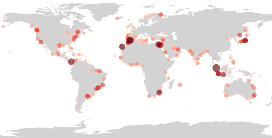
Figure 2: Spatial Distribution and Centrality of Global Maritime Ports. This map shows the locations of major ports around the world. The size of each circle corresponds to the importance and connectivity of the port within the global maritime network. Larger circles represent ports with higher centrality, indicating their significance in international trade and logistics.

4.1 Most central ports

Figure 2 shows the geographical placement of the most central ports (the size and darkness of the circle are proportional to the port centrality). Similarly, Table 3 shows the top 12 most central ports according to the definition of centrality given in Equation 4. Looking at the list in the table, we recognize some major worldwide container hubs and interesting entries. The top ports show a relatively wide geographical distribution. First in the top 12, Keppel in Singapore is in one of the busiest port areas of the world. Algeciras in Spain and Tangier in Morocco are located on the Strait of Gibraltar, the Mediterranean’s entrance passage and a stopping point for cargo ships. Puerto Cristobal (Colon) is a major ship hub on the Panama canal’s Atlantic entrance. Las Palmas is the largest port of the Canary Island, and it’s very central for its strategic position on the Atlantic Ocean.

Alexandria and El-Adabiya are two major Egyptian ports, respectively, on the Mediterranean and at the Suez Canal entrance in the Suez Gulf. Yokohama is one of the largest in Japan, and it is located in a very busy area at the entrance of the Tokyo port. The Durban port in South Africa is one of the largest container ports in the southern hemisphere. Jakarta and Gresik ports are the two largest in Indonesia, with Jakarta being one of the largest in Southeast Asia. Finally, Casablanca is the second largest in Morocco.

Rank	Port Name	Country	Centrality
1	KEPPEL	Singapore	10.594
2	ALGECIRAS	Spain	8.554
3	PUERTO CRISTOBAL	Panama	7.182
4	TANGIER	Morocco	6.742
5	LAS PALMAS	Spain	5.89
6	ALEXANDRIA	Egypt	4.941
7	YOKOHAMA	Japan	4.882
8	EL-ADABIYA	Egypt	4.823
9	GRESIK	Indonesia	4.542
10	DURBAN	South Africa	4.538
11	JAKARTA	Indonesia	4.4
12	CASABLANCA	Morocco	4.271

Table 3: Top 12 central ports and associated centrality values.

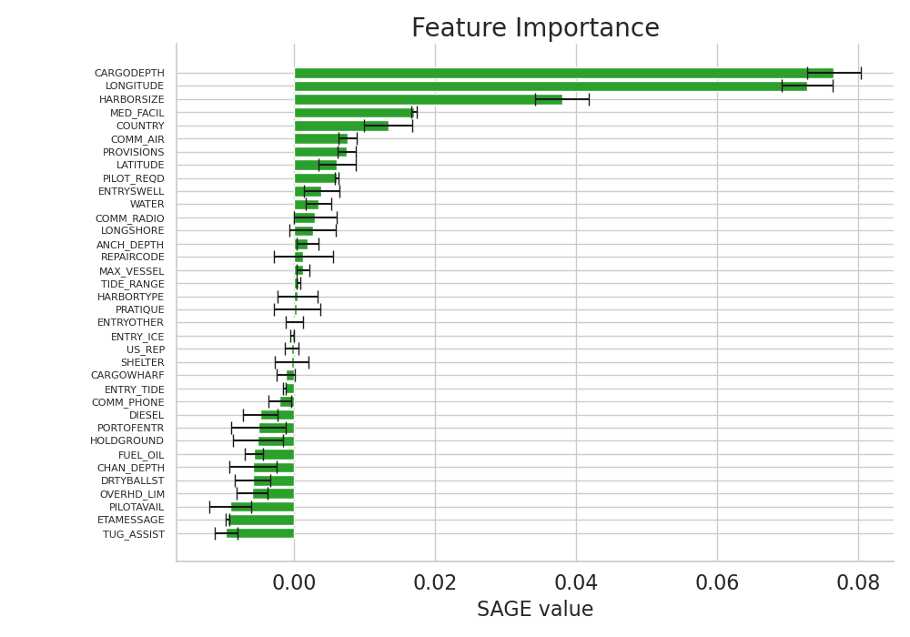
Figure 3: SAGE-Derived Feature Importance for Central Port Classification. This bar chart displays the feature importance values obtained using the SAGE (Shapley Additive Global Importance) method for classifying the top 10% most central ports. Key features such as CARGODEPTH, LONGITUDE, HARBORSIZE, and MED_FACIL show the highest importance, indicating their significant impact on the classification model. The error bars represent the variability in importance scores across different runs.

4.2 Assessing Model performances

To address our research questions, we need to quantitatively assess how accurately the random forest model can solve the binary classification task defined above (Section 3.5). To this end, we need a standard measure to understand how effectively assess whether a port is highly central in the graph of vessel voyages by just looking at the features of the port (RQ2). Moreover, to interpret the importance of features to solve this ML task, we need to ensure that the model picks up a pattern in the data instead of returning random guesses.

The area under the Receiver Operating Characteristic (ROC) curve is a popular indicator of prediction’s accuracy for binary classifications. The ROC curve is obtained by exploring various thresholds for a model’s binary classification and plotting the True Positive rate versus the False Positive rate. The resulting curve describes the performances of the binary classifier at hand, and the area under it is called the Area Under the Curve (AUC). In short, the closer the ROC is to the top left angle, the better the predictions, i.e., AUC close to $1$. For reference, a random classifier would be close to the diagonal line, with an AUC of $0.5$.

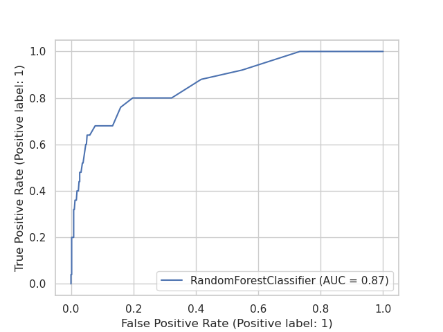
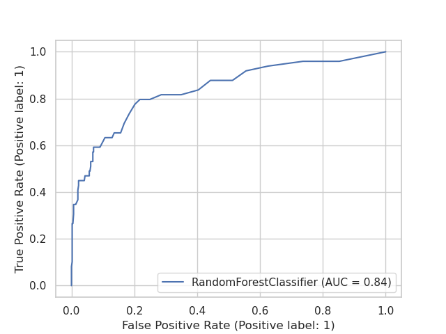
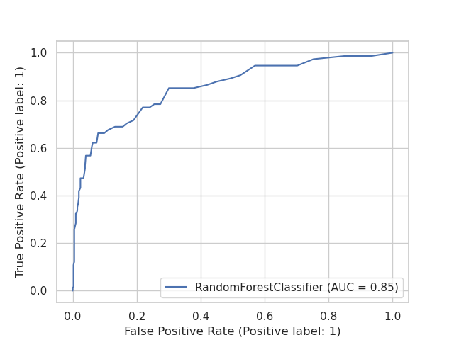
Figure 4: ROC curve from the random forest for the binary classification of most central ports. From left to right, we consider relevant ports, the ones on the $5\%$, $10\%$, $15\%$

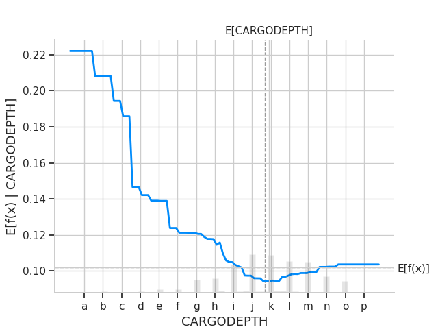
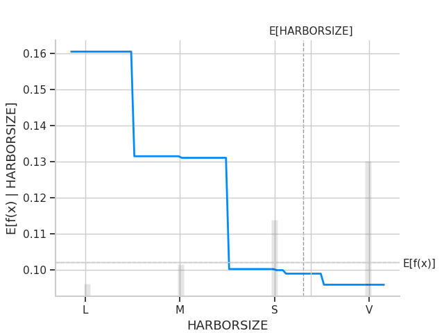
Figure 5: Partial dependence plots for the $3$ most important features according to SAGE, CARGODEPTH (top) and HARBOURSIZE (bottom). The vertical gray bar represents the average value of the feature. The blue partial dependence plot line is the average value of the model output when we fix the feature at hand to a given value. The grey histograms on the x-axis indicate the distribution of each feature.

For all the three threshold configurations for the most central ports ($5\%$, $10\%$, $15\%$), we show in Figure 4 the ROC curve for the binary classification of the most central ports, and the AUC in Table 4. The results confirm that the random forests obtain good results in the classification task and that the following analysis of feature importance is based on an accurate classifier, as the values of the AUC obtained are well above the $0.5$ ($0.84$, $0.88$, $0.87$, respectively) value that would be obtained by random classification.

4.3 Feature Importance

Subsequently, we analyze the results of the feature importance from the random forest model (RQ1); discussing predictability and codependence between the aggregated centrality and the port features but not causal relationships.

4.3.1 Global feature importance

In Figure 3, we show the SAGE values describing feature importance for the whole Ports Network when we considered the top $10\%$ of the ports as central. It emerges clearly that most important features in predicting the port centrality are CARGODEPTH, LONGITUDE, and HARBORSIZE.

Most Central Ports Threshold	5%	10%	15%
AUC value	$0.87$	$0.84$	$0.85$
CARGODEPTH	$0.02$	$0.04$	$0.08$
LONGITUDE	$0.07$	$0.04$	$0.07$
HARBORSIZE	$0.03$	$0.02$	$0.04$
COUNTRY	$0.01$	$0.03$	$0.01$
HAN_DEPTH	$0.02$	$0.02$	$0.006$

Table 4: The $5$ most important features and their SAGE values for predicting the most central ports in a binary classification

CARGODEPTH indicates the greatest depth for cargo vessels available in the port. A greater depth allows for large vessels to visit the port. For example, cargo vessels might require a depth greater than 12 meters, up to 25 meters for deeper ships. In the dataset, the depth is codified using letters from A to Q, with Q being the deepest. Each subsequent letter increases the depth by $5$ feet, approximately $1.5$ meters. For example, the letter H corresponds to $43$ feet (about $13$ meters). The information about the depth is the most useful for discriminating whether a cargo ship can enter the port.

Feature	Avg. Rank	Description
US REPRESENTATIVE	9.8	Indicates whether the United States maintains either civilian or military representation in the port.
DIRTY BALLAST	12.2	Whether a port has sufficient facilities for receiving oily or contaminated ballast.
PRATIQUE	12.6	Whether medical pratique is applied to vessels arriving in the port.
CARGODEPTH	13.8	Greatest depth for cargo vessels available in the port.
CHANNEL DEPTH	14.3	The depth of the deepest channel leading to the port.

Table 5: Top 5 non-geographical features ordered by their average rank

The HARBORSIZE is based on several factors, including area, facilities, and wharf space. It is codified into four categories: Large (L), Medium (M), Small (S), or Very Small (V). Similar to cargo depth, most cargo visits are focused on large ports, which makes this feature one of the most informative. Finally, LONGITUDE shows the importance of the geographical position of the port. It is interesting to note how longitude is more relevant than latitude in this context. One possible explanation is that most of the central ports (as graphically shown by Figure 2) lie in specific longitudinal areas (the Americas, Europe, and South-East Asia). Longitude is, therefore, a good discriminator for central ports.

While SAGE quantifies how important a feature is in improving the model’s prediction, it does not give us any information on the effect of different values of each variable on the model’s prediction. To gain some additional insight, in Figure 5, we show the partial dependency plots for the $3$ features that resulted globally most important. These plots show how the model prediction changes on average by changing the value of one variable. Notice that the dependencies are highly non-linear due to the non-linear nature of the random forest model we employed. Moreover, the CARGODEPTH data labeling is such that higher values correspond to lower values in meters. Hence, increasing the actual depth increases the likelihood that a port will be predicted as highly central. Finally, the correlation of a larger size of the harbor (HARBORSIZE) is evident, with large ports more likely to be central.

4.3.2 Local Feature Importance

Local feature importance measures the relevance of a feature in the classification of single input items. To provide a summary of what features are more locally important, we ranked them according to their average contribution to each port’s classification. Intuitively, the average ranking would measure how consistently a feature contributes to a port’s positive classification. In general, the geographical features ranked the highest. Apart from those, Table 5 shows the top 5 non-geographical features. Interestingly, a “political" feature ranks first. Then, services such as medical procedures and management of contaminated materials are typical of international ports and could differentiate the port centrality. Finally, port depths directly correlate with the ability of the port to allow entrance for large cargo ships.

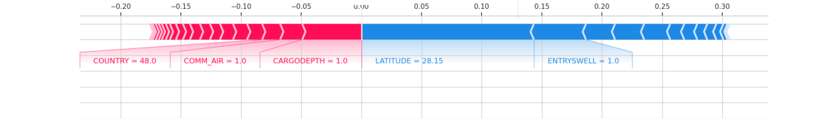
Figure 6: SHAP Force Plot for Feature Contributions at Las Palmas Port. This force plot visualizes the impact of various features on the classification outcome for the Las Palmas port case. Features contributing to a correct classification are highlighted in red, while those contributing to an incorrect classification are shown in blue. Notable features include COUNTRY, COMM_AIR, CARGODEPTH, LATITUDE, and ENTRYSWELL, with their respective values influencing the model’s prediction.

Another interesting analysis is looking at single ports and how their features correlate with their importance locally. Figure 6 shows the Las Palmas port. CARGODEPTH, COMM_AIR (indicates whether airport communications are available), and COUNTRY are features that help classify them. Contrarily, its latitude and ENTRY SWELL (binary, whether there is a natural factor restricting the entrance of vessels) are not favorable features for this port.

5 Conclusion

This paper presents an approach based on machine learning explainability to evaluate the most important features of ports and predict their significance. To do this, we constructed a Ports Network with three years of worldwide data, in which the significance of a port is determined by the combination of centrality measures commonly used in the literature. We performed a machine learning task to predict the port’s importance using publicly available features and analyzed which features are most useful for inference.

It turns out that geographical features help the most in discerning important ports. This is a direct and expected result, as ports are infrastructures connecting coastal locations with specific geographical properties. Apart from geographical features, the features that inform about the depth of different port areas (such as the entrance depth and the depth of the piers) are the most relevant to an accurate prediction. These results confirm the expected, as the analysis is based on cargo ships requiring deep water.

This paper also paves the way for similar research on other types of vessels and transportation modalities, such as passenger or leisure vessels. Also, identifying the features of central maritime ports can foster research on developing new or existing ports and provide a tool to study inter-port and regional relationships. These points provide potential research directions for extending this study.

Declaration of competing interest

The authors declare no conflicts of interest.

Data Licensing and Disclosure

The research described in this paper used data acquired from Spire under MERIDIAN’s fair-use and non-disclosure data license. This high-resolution research data is hosted at the Institute for Big Data Analytics (IBDA) at Dalhousie University. Due to licensing agreements, we are unable to share the raw data. However, we can provide a trained model and the means to retrain the models using open-source data from similar maritime regions.

References

- Carlini et al. [2021] Emanuele Carlini, Vinicius Monteiro de Lira, Amilcar Soares, Mohammad Etemad, Bruno Brandoli, and Stan Matwin. Understanding evolution of maritime networks from automatic identification system data. GeoInformatica, pages 1–25, 2021.
- Varlamis et al. [2019] Iraklis Varlamis, Konstantinos Tserpes, Mohammad Etemad, Amílcar Soares Júnior, and Stan Matwin. A network abstraction of multi-vessel trajectory data for detecting anomalies. In EDBT/ICDT Workshops, 2019.
- Varlamis et al. [2021] Iraklis Varlamis, Ioannis Kontopoulos, Konstantinos Tserpes, Mohammad Etemad, Amilcar Soares, and Stan Matwin. Building navigation networks from multi-vessel trajectory data. GeoInformatica, 25(1):69–97, 2021.
- Ducruet et al. [2010a] César Ducruet, Céline Rozenblat, and Faraz Zaidi. Ports in multi-level maritime networks: evidence from the atlantic (1996–2006). Journal of Transport geography, 18(4):508–518, 2010a.
- Laxe et al. [2012] Fernando González Laxe, Maria Jesus Freire Seoane, and Carlos Pais Montes. Maritime degree, centrality and vulnerability: port hierarchies and emerging areas in containerized transport (2008–2010). Journal of Transport Geography, 24:33–44, 2012.
- Álvarez et al. [2021] Nicanor García Álvarez, Belarmino Adenso-Díaz, and Laura Calzada-Infante. Maritime traffic as a complex network: A systematic review. Networks and Spatial Economics, pages 1–31, 2021.
- Del Mondo et al. [2021] Géraldine Del Mondo, Peng Peng, Jérôme Gensel, Christophe Claramunt, and Feng Lu. Leveraging spatio-temporal graphs and knowledge graphs: Perspectives in the field of maritime transportation. ISPRS International Journal of Geo-Information, 10(8):541, 2021.
- Zhang et al. [2023] Fan Zhang, Yihao Liu, Lei Du, Floris Goerlandt, Zhongyi Sui, and Yuanqiao Wen. A rule-based maritime traffic situation complex network approach for enhancing situation awareness of vessel traffic service operators. Ocean Engineering, 284:115203, 2023. ISSN 0029-8018. https://doi.org/10.1016/j.oceaneng.2023.115203.
- Cheung et al. [2020] Kam-Fung Cheung, Michael GH Bell, Jing-Jing Pan, and Supun Perera. An eigenvector centrality analysis of world container shipping network connectivity. Transportation Research Part E: Logistics and Transportation Review, 140:101991, 2020.
- Li et al. [2021] Jing Li, Xuantong Wang, and Tong Zhang. Sequence-based centrality measures in maritime transportation networks. IET Intelligent Transport Systems, 14(14):2042–2051, 2021.
- Wang and Cullinane [2016] Yuhong Wang and Kevin Cullinane. Determinants of port centrality in maritime container transportation. Transportation Research Part E: Logistics and Transportation Review, 95:326–340, 2016.
- Rodrigues [2019] Francisco Aparecido Rodrigues. Network centrality: an introduction. In A mathematical modeling approach from nonlinear dynamics to complex systems, pages 177–196. Springer, 2019.
- Yang et al. [2019] Dong Yang, Lingxiao Wu, Shuaian Wang, Haiying Jia, and Kevin X Li. How big data enriches maritime research–a critical review of automatic identification system (ais) data applications. Transport Reviews, 39(6):755–773, 2019.
- Wang et al. [2019] Zhihuan Wang, Christophe Claramunt, and Yinhai Wang. Extracting global shipping networks from massive historical automatic identification system sensor data: a bottom-up approach. Sensors, 19(15):3363, 2019.
- Song et al. [2024] Ruixin Song, Gabriel Spadon, Ronald Pelot, S. Matwin, and Amílcar Soares. Enhancing global maritime traffic network forecasting with gravity-inspired deep learning models. arXiv preprint arXiv:2401.13098, 2024. 10.48550/arXiv.2401.13098.
- McWhinnie et al. [2021] Lauren H. McWhinnie, Patrick D. O’Hara, Casey Hilliard, Nicole Le Baron, Leh Smallshaw, Ronald Pelot, and Rosaline Canessa. Assessing vessel traffic in the salish sea using satellite ais: An important contribution for planning, management and conservation in southern resident killer whale critical habitat. Ocean & Coastal Management, 200:105479, 2021. ISSN 0964-5691. https://doi.org/10.1016/j.ocecoaman.2020.105479. URL https://www.sciencedirect.com/science/article/pii/S0964569120303860.
- Spadon et al. [2024] Gabriel Spadon, Jay Kumar, Derek Eden, Josh van Berkel, Tom Foster, Amilcar Soares, Ronan Fablet, Stan Matwin, and Ronald Pelot. Multi-path long-term vessel trajectories forecasting with probabilistic feature fusion for problem shifting. arXiv preprint arXiv:2310.18948, 2024. 10.48550/arXiv.2310.18948.
- Alam et al. [2024] M. Alam, Gabriel Spadon, Mohammad Etemad, Luis Torgo, and E. Milios. Enhancing short-term vessel trajectory prediction with clustering for heterogeneous and multi-modal movement patterns. Ocean Engineering, 308:118303, September 2024. ISSN 0029-8018. 10.1016/j.oceaneng.2024.118303.
- Covert et al. [2020] Ian Covert, Scott M Lundberg, and Su-In Lee. Understanding global feature contributions with additive importance measures. Advances in Neural Information Processing Systems, 33:17212–17223, 2020.
- Lundberg and Lee [2017] Scott M Lundberg and Su-In Lee. A unified approach to interpreting model predictions. Advances in neural information processing systems, 30, 2017.
- Tovar et al. [2015] Beatriz Tovar, Rubén Hernández, and Héctor Rodríguez-Déniz. Container port competitiveness and connectivity: The canary islands main ports case. Transport Policy, 38:40–51, 2015.
- Ducruet et al. [2010b] César Ducruet, Sung-Woo Lee, and Adolf KY Ng. Centrality and vulnerability in liner shipping networks: revisiting the northeast asian port hierarchy. Maritime Policy & Management, 37(1):17–36, 2010b.
- Montes et al. [2012] Carlos Pais Montes, Maria Jesus Freire Seoane, and Fernando González Laxe. General cargo and containership emergent routes: A complex networks description. Transport Policy, 24:126–140, 2012.
- Seoane et al. [2013] Maria Jesus Freire Seoane, Fernando González Laxe, and Carlos Pais Montes. Foreland determination for containership and general cargo ports in europe (2007–2011). Journal of Transport Geography, 30:56–67, 2013.
- Tran and Haasis [2014] Nguyen Khoi Tran and Hans-Dietrich Haasis. Empirical analysis of the container liner shipping network on the east-west corridor (1995–2011). NETNOMICS: Economic Research and Electronic Networking, 15(3):121–153, 2014.