Designing Chaotic Attractors:
A Semi-supervised Approach
Abstract
Chaotic dynamics are ubiquitous in nature and useful in engineering, but their geometric design can be challenging. Here, we propose a method using reservoir computing to generate chaos with a desired shape by providing a periodic orbit as a template, called a skeleton. We exploit a bifurcation of the reservoir to intentionally induce unsuccessful training of the skeleton, revealing inherent chaos. The emergence of this untrained attractor, resulting from the interaction between the skeleton and the reservoir’s intrinsic dynamics, offers a novel semi-supervised framework for designing chaos.
pacs:
Valid PACS appear hereChaotic dynamics are prevalent in nature, including biological neural systems [1, 2, 3], and are applied in engineering, such as for random number generation [4, 5], communication systems [6, 7], optimization [8, 9], deep learning [10, 11], and robot control [12, 13, 14].
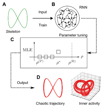
A notable challenge is designing the geometric shapes of chaotic attractors, for which no practical methods have been proposed so far, to the best of our knowledge. In this paper, as shown in Fig. 1, we propose a method using the reservoir computing (RC) framework [15, 16, 17]. In this method, a periodic orbit, which we call a skeleton, defines the contour of the output trajectory. Training the reservoir with the skeleton under certain parameter values yields an autonomous system, where the maximum Lyapunov exponent (MLE) exceeds zero, while the trajectory mimics the shape of the skeleton, indicating periodic chaos.
The proposed method utilizes attractor reconstruction with RC [18, 19], which is achieved through one-step-ahead prediction of the target inputs and closed-loop operation. The premise of RC is to use a fixed nonlinear dynamical system of the following form:
| (1a) | ||||
| (1b) | ||||
Here, the reservoir (1a) is an -dimensional system with a -dimensional input, where and represent the reservoir state and the input, respectively. The output is defined as a linear combination of . Typically, recurrent neural networks (RNNs) are employed as reservoirs. The readout layer is constructed so that using ridge regression with following process: the reservoir is driven by the teacher input (teacher forcing), and the set of the response is obtained for steps, with the initial steps discarded. This yields the paired learning data:
| (2) |
Then, is determined by
| (3) |
where is the regularization parameter. By feeding back the predicted output as the alternative input, the system acquires autonomous dynamics:
| (4) |
where the initial state is the final state of the teacher forcing. The well-trained system replicates the target attractor, mimicking its ergodic characteristics and providing estimates of dynamical quantities, such as Lyapunov exponents (LE) [18, 20]. Conversely, this autonomous system may exhibit some properties not present in the target, termed untrained attractors [18, 21].
The attractor shown in Fig. 1D is a chaotic untrained attractor. We demonstrate that the emergence of such attractors can be induced by appropriate parameter selection in the learning periodic sequences and formalize this fact as a method for designing chaotic attractors. Importantly, the obtained chaos is formed by integrating the teacher information and the intrinsic dynamical properties of the reservoir. Therefore, this method can be considered a novel “semi-supervised” framework.
As a case study on learning periodic orbits, we consider the Lissajous curve shown in Fig. 1A. In this paper, the reservoir is a leaky integrator echo state network (LESN) [22], described by
| (5) |
where is the leaky rate, and is an element-wise function. Here, is a random matrix whose elements follow a standard normal distribution, and it is scaled to have a spectral radius at unity. Thus, is the spectral radius of the internal connection matrix . The input layer is a random matrix whose elements follow a uniform distribution in , and represents the input intensity.
The dynamical properties of a random RNN without input depend largely on the spectral radius of its internal connection matrix [23, 24]. For an LESN, we introduce the effective spectral radius [22] as follows:
| (6) |
Typically, the MLE of the input-free LESN increases with and exceeds zero at unity, as shown in Fig. S1 in the Supplementary Material. To ensure reservoir convergence, Jaeger et al. [22] recommend keeping in practice. However, chaos in RNNs can be suppressed by external inputs [25]. Even with , successful learning is feasible if the input-driven reservoir exhibits convergence properties, which is guaranteed by the negative conditional Lyapunov exponent (CLE) [26, 18].
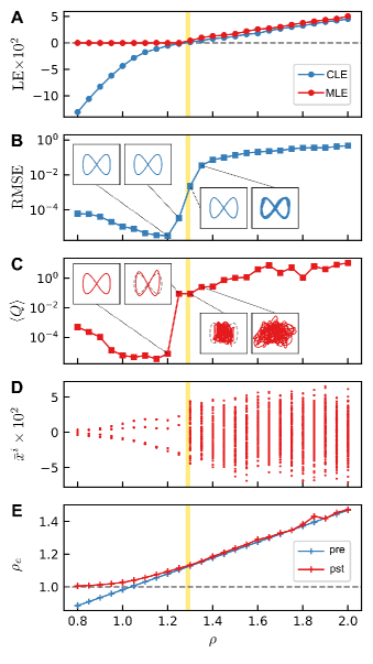
As shown in Fig. 2A, when the parameters are fixed at , the CLE with Lissajous curve input increases with and the sign changes in . This region corresponds to the “edge of chaos” of the driven system, indicating the limit of chaos suppression [27]. In this paper, the range of with positive CLEs are referred to as the “chaotic region,” and those with negative CLEs as the “convergent region,” respectively.
As shown in Fig. 2B, the performance of the open-loop prediction was evaluated using the root mean square error, . The prediction can be considered successful when . The range meets this criterion, with CLEs being negative or close to zero. The error decreases until and then increases. Although the prediction is successful for and , the excessively slow convergence of the driven reservoir likely negatively impacts the task. Additionally, a negative CLE does not guarantee a successful prediction and reconstruction. They also depend on the reservoir’s short-term memory and information processing capacity, which can be influenced by [27]. Thus, the range of successful learning for depends on the selected target.
The trained closed-loop model is described by
| (7) | ||||
Here, the learning can be understood as a change in the matrix from to by adding the readout matrix [28]. We fix and compare the properties of the closed-loop model for each . To evaluate the shape of the output, we introduce an indicator , which is obtained by eliminating the time variable from . This index is zero on the Lissajous curve, with a larger value indicating greater deviation. Here, we use the time average . If , the trajectory is “along” the target curve. As shown in Figs. 2A and 2C, in the chaotic region (), the MLEs have positive values, and the learning fails. In contrast, in the convergence region (), the MLEs are zero, indicating a periodic attractor. Especially for , trajectories with are obtained.
Figure 2D displays the extrema of the node averages of the internal states in the last 2,000 steps of the 10,000-step trajectory for each . Because the post-training matrix is a function of , Fig. 2D can be interpreted as a bifurcation diagram of the autonomous system (7) with respect to the bifurcation parameter , showing the parametric continuity of the periodic orbits and the transition to chaos.
Additionally, we introduce the post-training effective spectral radius:
| (8) |
As shown in Fig. 2E, is clearly larger than for . Approaching the edge of chaos, converges to , and for , is nearly equal to . Here, it can be inferred that in the convergence region where clearly increases, learning modifies the convergence property of the reservoir, realizing the periodic attractor as a “supervised” attractor. Conversely, in the chaotic region, this operation fails, and the reservoir’s chaos is foregrounded, inducing an untrained chaotic attractor, even if the open-loop prediction roughly succeeds.
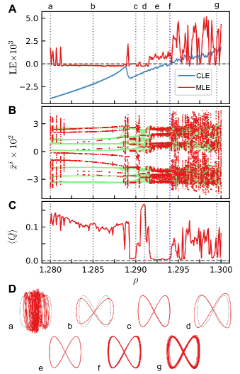
We closely explore the vicinity of the edge of chaos, , expecting a bifurcation structure connecting the supervised periodic orbits with the deformed chaotic attractors. As shown in Fig. 3A, the sign of CLE reverses at . We denote this point as and focus on , where the learning results are unstable. As shown in Fig. 3A, windows of periodic solutions with alternate with chaotic regions with . Figure 3B is a bifurcation diagram obtained similarly to Fig. 2D, but it also includes the first 2,000 steps. The trajectories appearing as continuous light green curves in the range correspond to the long transient on , implying that the Lissajous curve exists as an unstable orbit (Figs. 3Da and 3Db). This orbit stabilizes (Fig. 3Dc) and destabilizes again (Fig. 3Dd). In the region up to after the untrained periodic orbit destabilizes, we observe the chaotic attractors with and (Figs. 3De and 3Df).
These chaotic attractors appear as multiple separated bands in Fig. 3B, indicating periodic/band chaos in terms of typical discrete-time dynamical systems. They likely appear due to period-doubling bifurcations.
The instability of results in this region can be attributed to the slow convergence of the driven system. Therefore, the length of the truncated transient, , can act as a bifurcation parameter, which is discussed in the Supplementary Material.
Above , the bands collapse, suggesting that a crisis occurs at this point. It is worth noting that even at , a similar periodic chaos is found, for example, at , as shown in Fig. 3Dg. However, because the chaos in the driven system is not suppressed, the bifurcation structure in this region should be more complex than that for .
From the above result, chaotic attractors with shapes along the Lissajous curve can be seen in the bifurcation process, in which the reconstruction of the periodic orbits collapses with the emergence of untrained chaotic attractors. We refer to the points where supervised periodic orbits are reconstructed as the “supervised points” and the points where chaotic attractors with shapes along the skeleton emerge as the “semi-supervised points” .
In the trials using the Lissajous curve, can be found between and with different realizations of the random matrices and . It also holds when the skeleton is changed, as shown in Fig. S4 in the Supplementary Material.
Figure 4A shows the chaotic attractor generated with the Van der Pol oscillator. It is worth noting that the time series is classified as a sequence of quasi-periodic orbits in discrete time, while the Lissajous curve is periodic orbits. Despite this difference, consistent results were obtained. Furthermore, Fig. 4B shows the results using the hand-drawn closed curve, demonstrating that similar phenomena can be observed even when no explicit equations are known for the skeleton.
The generation of semi-supervised points can be explained from the following two perspectives. First, as previously discussed, fully supervised attractors are obtained with sufficiently fast convergence, while in chaotic regions, the reservoir chaos is foregrounded. Given a bifurcation structure by linking these two points, it is plausible that attractors in the intermediate region may display properties midway between the two. Specifically, the generated chaos is thought to arise from the supervised periodic orbits becoming chaotic through a cascade of period-doubling bifurcation. Therefore, one trivial requirement is the existence of .
Second, the CLE is crucial. According to Hart [29], the LEs of the well-trained reservoir reconstructing a chaotic system provides reliable estimates of the target’s LEs only for those larger than the driven reservoir’s CLE. Negative LEs below the CLE tend to approximate those of the driven system rather than the ground truth. Therefore, accurate reconstruction requires a sufficiently negative CLE. Although we focus on periodic orbits, this fact is important. For example, when embedding a limit cycle, the MLE should be zero, and other exponents should be negative. If the CLE is zero, even with successful prediction, the non-convergence of the driven system makes the orbit unstable in the closed-loop state.
Moreover, the prediction always involves some errors, which are fed back into the reservoir and act as noise in subsequent predictions. The accumulation of this noise determines the qualitative difference between the open-loop attractor and the closed-loop attractor . If the prediction is successful, the evolution of approximates with small noise. Fast convergence of the driven system prevents error accumulation, resulting in . Conversely, large prediction errors or slow convergence may lead to error accumulation and destabilize the orbit of . Therefore, it is plausible that the behavior of trajectories near the skeleton in a closed-loop state is determined by the balance between prediction errors and the convergence of the driven system. Thus, by appropriately selecting to determine the CLE, generating chaos near the skeleton can be achieved. However, the exploration of the corresponding parameters is heuristic.
As shown in Fig. 1, the procedure for identifying the semi-supervised points is formulated as follows:
-
1.
Prepare a periodic time series as the skeleton that defines the shape of the output.
-
2.
Prepare the reservoir with fixed parameters .
-
3.
Roughly identify in this setting.
-
4.
Repeat learning for to discover . If not found, return to step 2 and modify the fixed setting.
-
5.
Explore the interval
Step 4 can be simplified using a binary search. Step 5 essentially repeats learning and manually evaluates the results, but automation is possible if a geometric evaluation index like is available. However, as shown in Fig. 3, there may be multiple windows of periodic solutions, so a somewhat detailed search is required.
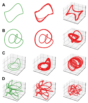
The application results for three-dimensional data are shown in Fig. 4C and 4D. The trial shown in Fig. 4C uses a limit cycle obtained from the Rössler system, and some of the obtained attractors resemble the chaotic attractors seen in the original system, which is discussed in the Supplementary Material. The skeleton in Fig. 4D is constructed by repeating sound waves produced by three keys on a piano. The generated chaotic output sounds similar to the original when played as audio.
Similar periodic chaos might be achievable using conventional supervised learning with RNNs. However, it requires minimizing the prediction error while ensuring , leading to a significantly complex design and computation of the loss function [30].
One application of the method is in the control of systems, including robotics. For example, chaos can be utilized in robot motor commands to avoid deadlock or to escape when a limb becomes trapped in a confined space [31]. In such cases, the employed chaotic trajectories should be designed with consideration for the robot’s body morphology and desired locomotion pattern. Additionally, periodic chaos can aid in synchronizing nonlinear systems. Carroll et al. [32] discussed systems driven by periodic inputs that behave with -multiple periods of the driving signal. Their phase depends on initial conditions, which is problematic when driving multiple systems with the same input to achieve synchronized -period behavior, such as the coordination of robot parts that employ nonlinear materials. According to the authors, this issue can be resolved by using pseudo-periodic inputs with chaotic or stochastic variations instead of periodic inputs. Our method can help generate these pseudo-periodic inputs, which resemble the original input.
Finally, although this paper focuses on a method employing an LESN, future work could extend to physical reservoir computing [33]. This is particularly relevant for autonomous control systems that expect both appropriate behavior and emergent properties [34]. In such cases, a control framework leveraging the system’s intrinsic dynamical properties can be crucial.
Acknowledgements.
K. A. was supported by Moonshot R&D Grant Number JPMJMS2021, the institute of AI and Beyond of UTokyo, the International Research Center for Neurointelligence (WPI-IRCN) at The University of Tokyo Institutes for Advanced Study (UTIAS), JSPS KAKENHI Grant Number JP20H05921, Cross-ministerial Strategic Innovation Promotion Program (SIP), and the 3rd period of the SIP “Smart energy management system” Grant Number JPJ012207References
- Hayashi et al. [1982] H. Hayashi, S. Ishizuka, M. Ohta, and K. Hirakawa, Chaotic behavior in the onchidium giant neuron under sinusoidal stimulation, Physics Letters A 88, 435 (1982).
- Aihara et al. [1986] K. Aihara, T. Numajiri, G. Matsumoto, and M. Kotani, Structures of attractors in periodically forced neural oscillators, Physics Letters A 116, 313 (1986).
- Freeman [1987] W. J. Freeman, Simulation of chaotic eeg patterns with a dynamic model of the olfactory system, Biological cybernetics 56, 139 (1987).
- Akashi et al. [2022] N. Akashi, K. Nakajima, M. Shibayama, and Y. Kuniyoshi, A mechanical true random number generator, New Journal of Physics 24, 013019 (2022).
- Uchida et al. [2008] A. Uchida, K. Amano, M. Inoue, K. Hirano, S. Naito, H. Someya, I. Oowada, T. Kurashige, M. Shiki, S. Yoshimori, et al., Fast physical random bit generation with chaotic semiconductor lasers, Nature Photonics 2, 728 (2008).
- Argyris et al. [2005] A. Argyris, D. Syvridis, L. Larger, V. Annovazzi-Lodi, P. Colet, I. Fischer, J. Garcia-Ojalvo, C. R. Mirasso, L. Pesquera, and K. A. Shore, Chaos-based communications at high bit rates using commercial fibre-optic links, Nature 438, 343 (2005).
- Boccaletti et al. [2000] S. Boccaletti, C. Grebogi, Y.-C. Lai, H. Mancini, and D. Maza, The control of chaos: theory and applications, Physics reports 329, 103 (2000).
- Chen and Aihara [1995] L. Chen and K. Aihara, Chaotic simulated annealing by a neural network model with transient chaos, Neural networks 8, 915 (1995).
- Kong and Tao [2020] L. Kong and M. Tao, Stochasticity of deterministic gradient descent: Large learning rate for multiscale objective function, Advances in Neural Information Processing Systems 33, 2625 (2020).
- Inoue et al. [2022] K. Inoue, S. Ohara, Y. Kuniyoshi, and K. Nakajima, Transient chaos in bidirectional encoder representations from transformers, Physical Review Research 4, 013204 (2022).
- Liu et al. [2024] S. Liu, N. Akashi, Q. Huang, Y. Kuniyoshi, and K. Nakajima, Exploiting chaotic dynamics as deep neural networks (2024), arXiv:2406.02580 [cs.NE] .
- Namikawa et al. [2011] J. Namikawa, R. Nishimoto, and J. Tani, A neurodynamic account of spontaneous behaviour, PLoS computational biology 7, e1002221 (2011).
- Laje and Buonomano [2013] R. Laje and D. V. Buonomano, Robust timing and motor patterns by taming chaos in recurrent neural networks, Nature neuroscience 16, 925 (2013).
- Inoue et al. [2020] K. Inoue, K. Nakajima, and Y. Kuniyoshi, Designing spontaneous behavioral switching via chaotic itinerancy, Science advances 6, eabb3989 (2020).
- Jaeger [2001] H. Jaeger, The “echo state” approach to analysing and training recurrent neural networks-with an erratum note, Bonn, Germany: German National Research Center for Information Technology GMD Technical Report 148, 13 (2001).
- Maass et al. [2002] W. Maass, T. Natschläger, and H. Markram, Real-time computing without stable states: A new framework for neural computation based on perturbations, Neural computation 14, 2531 (2002).
- Nakajima and Fischer [2021] K. Nakajima and I. Fischer, Reservoir Computing (Springer, 2021).
- Lu et al. [2018] Z. Lu, B. R. Hunt, and E. Ott, Attractor reconstruction by machine learning, Chaos: An Interdisciplinary Journal of Nonlinear Science 28 (2018).
- Hart et al. [2020] A. Hart, J. Hook, and J. Dawes, Embedding and approximation theorems for echo state networks, Neural Networks 128, 234 (2020).
- Pathak et al. [2017] J. Pathak, Z. Lu, B. R. Hunt, M. Girvan, and E. Ott, Using machine learning to replicate chaotic attractors and calculate lyapunov exponents from data, Chaos: An Interdisciplinary Journal of Nonlinear Science 27, 121102 (2017).
- Flynn et al. [2021] A. Flynn, V. A. Tsachouridis, and A. Amann, Multifunctionality in a reservoir computer, Chaos: An Interdisciplinary Journal of Nonlinear Science 31, 013125 (2021).
- Jaeger et al. [2007] H. Jaeger, M. Lukoševičius, D. Popovici, and U. Siewert, Optimization and applications of echo state networks with leaky-integrator neurons, Neural networks 20, 335 (2007).
- Sompolinsky et al. [1988] H. Sompolinsky, A. Crisanti, and H.-J. Sommers, Chaos in random neural networks, Physical review letters 61, 259 (1988).
- Cessac and Samuelides [2007] B. Cessac and M. Samuelides, From neuron to neural networks dynamics, The European Physical Journal Special Topics 142, 7 (2007).
- Molgedey et al. [1992] L. Molgedey, J. Schuchhardt, and H. G. Schuster, Suppressing chaos in neural networks by noise, Physical review letters 69, 3717 (1992).
- Verstraeten et al. [2007] D. Verstraeten, B. Schrauwen, M. d’Haene, and D. Stroobandt, An experimental unification of reservoir computing methods, Neural networks 20, 391 (2007).
- Haruna and Nakajima [2019] T. Haruna and K. Nakajima, Optimal short-term memory before the edge of chaos in driven random recurrent networks, Physical Review E 100, 062312 (2019).
- Sussillo and Abbott [2012] D. Sussillo and L. Abbott, Transferring learning from external to internal weights in echo-state networks with sparse connectivity, PLoS One 7, e37372 (2012).
- Hart [2024] J. D. Hart, Attractor reconstruction with reservoir computers: The effect of the reservoir’s conditional lyapunov exponents on faithful attractor reconstruction, Chaos: An Interdisciplinary Journal of Nonlinear Science 34 (2024).
- Mikhaeil et al. [2022] J. Mikhaeil, Z. Monfared, and D. Durstewitz, On the difficulty of learning chaotic dynamics with rnns, Advances in Neural Information Processing Systems 35, 11297 (2022).
- Steingrube et al. [2010] S. Steingrube, M. Timme, F. Wörgötter, and P. Manoonpong, Self-organized adaptation of a simple neural circuit enables complex robot behaviour, Nature physics 6, 224 (2010).
- Carroll and Pecora [1993] T. L. Carroll and L. M. Pecora, Using chaos to keep period-multiplied systems in phase, Physical Review E 48, 2426 (1993).
- Nakajima [2020] K. Nakajima, Physical reservoir computing―an introductory perspective, Japanese Journal of Applied Physics 59, 060501 (2020).
- Akashi et al. [2024] N. Akashi, Y. Kuniyoshi, T. Jo, M. Nishida, R. Sakurai, Y. Wakao, and K. Nakajima, Embedding bifurcations into pneumatic artificial muscle, Advanced Science , 2304402 (2024).