Multi-object Data Integration in the Study of Primary Progressive Aphasia

Abstract

This article focuses on a multi-modal imaging data application where structural/anatomical information from gray matter (GM) and brain connectivity information in the form of a brain connectome network from functional magnetic resonance imaging (fMRI) are available for a number of subjects with different degrees of primary progressive aphasia (PPA), a neurodegenerative disorder (ND) measured through a speech rate measure on motor speech loss. The clinical/scientific goal in this study becomes the identification of brain regions of interest significantly related to the speech rate measure to gain insight into ND patterns. Viewing the brain connectome network and GM images as objects, we develop an integrated object response regression framework of network and GM images on the speech rate measure. A novel integrated prior formulation is proposed on network and structural image coefficients in order to exploit network information of the brain connectome while leveraging the interconnections among the two objects. The principled Bayesian framework allows the characterization of uncertainty in ascertaining a region being actively related to the speech rate measure. Our framework yields new insights into the relationship of brain regions associated with PPA, offering a deeper understanding of neuro-degenerative patterns of PPA. The supplementary file adds details about posterior computation and additional empirical results.

Key Words: Bayesian inference; brain connectome; functional magnetic resonance imaging; gray matter; multi-modal imaging; primary progressive aphasia; spike and slab prior.

1 Introduction

This article is motivated by a clinical application on patients suffering from brain loss due to Primary Progressive Aphasia (PPA), a neurodegenerative disorder (ND) characterized by loss of language ability that shares pathological signatures with Alzheimer’s disease and frontotemporal dementia. Despite the devastating toll PPA effects on a patient’s ability to communicate, it is far less widely studied than other NDs, and as a result, research cohorts contain modest sample sizes. We consider the nonfluent/agrammatic variant of PPA (nfvPPA) characterized by motor speech and grammar loss and left inferior frontal atrophy (Gorno-Tempini et al., 2008). Multi-modal imaging data are available for each of these PPA patients which include: (a) brain network information and (b) brain structural information. Brain networks consider each region of interest (ROI) as a network node and quantifies the connectivity between the pairs of network nodes using functional magnetic resonance imaging (fMRI). Brain structural information is obtained using structural magnetic resonance imaging (sMRI), e.g., gray matter (GM) images over brain volumetric pixels (voxels). Both images are collected on a common brain atlas which segments a human brain into different ROIs, with each ROI containing a number of voxels. A speech rate score is available for all these patients to measure the degree of their motor speech loss due to PPA.

The major scientific goals of the study are twofold, (a) to estimate regression relationships between the speech rate and the two imaging modalities; and (b) to identify ROIs significantly related to the speech rate, and thus infer the ND patterns for PPA.

To this end, the identification of statistically influential ROIs via a principled modeling framework is necessary to yield results that are scientifically interpretable in the lingua franca of well-characterized brain anatomy and function. While many ROI-based inferential techniques are constrained by considering the ROI as the most basic unit of analysis, the PPA data application allows for additional granular inference at the level of the voxel which will provide neuroscientists with the dual ability to frame results at the macro level of the ROI and probe the micro voxel-level signals that drive these results. To our knowledge, this article proposes the first statistical framework that allows for flexibility of macro and micro inference on multi-object imaging data which is urgently needed in the neuroscience community (Calhoun and Sui, 2016). Uncertainty quantification regarding the inference on influential regions becomes crucial since the analysis only involves a limited number of rarely studied PPA patients.

This article addresses the inferential objective by formulating a multi-modal regression framework with the brain network (defined over brain ROIs) and structural images (defined over brain voxels) as two sets of responses and the speech rate as the predictor. A hierarchical Bayesian approach is adopted wherein an integrated prior structure on coefficients of the speech rate corresponding to the structural and network objects (hereon referred to as the structural and network coefficients, respectively) is developed to allow the information in separate image objects to complement and reinforce each other in their relation to the scalar predictor. To elaborate, we begin with a common brain atlas for both image objects to ensure an organizing principle that links together structural and network information via a shared set of ROIs and a group of voxels within each ROI. The integrated prior on network and structural coefficients are constructed respecting the hierarchical constraint which ensures all voxels within an ROI uninfluential if the ROI is un-influential (see Section 3.2). While we do not explicitly make use of the structural information in the GM images by careful spatial modeling of the GM image coefficient, it partially exploits the structural information by imposing the hierarchical constraint in the prior construction. The problem of identifying influential ROIs is cast under a nonlinear variable selection framework, wherein latent activation indicators corresponding to all ROIs are shared among both sets of coefficients to enforce that all voxels from a particular ROI and all network edges connected to that particular ROI have no relationship with the predictor when the activation indicator corresponding to the ROI is zero. As a byproduct of our construction, symmetry and transitivity property (Hoff, 2005) of the un-directed network object is preserved, as discussed in Section 3.2. The prior construction achieves efficient computation, identifies influential ROIs and voxels within an influential ROI which are key to studying neuronal degradation, and produces well-calibrated interval estimates for the multi-modal regression coefficients. Moreover, our framework attaches uncertainty in identifying these ROIs and offers improved inference over regression methods with a single imaging modality.

There is a dearth of principled Bayesian literature addressing the inferential objectives of the motivating application, and our proposal is arguably the first Bayesian multi-object regression approach to answer the inferential questions stated before. We now provide a brief overview of the available literature to contrast them with our proposal. In the course to determine the association between network or structural objects and the speech rate score, the most popular approach estimates the association between each network edge or GM voxel and the language score independently, providing a p-value “map” (Lazar, 2008, 2016), after adjusting for multiple comparisons to identify “significant” ROIs. Such approaches have key disadvantages relative to methods that take into account the integrated impact of all network edges and voxels of the GM images simultaneously, as demonstrated in Section 5.

One can possibly proceed to vectorize both objects and regress them jointly on the speech rate, leading to a high dimensional vector response regression problem. This approach can take advantage of the recent developments in high dimensional multivariate reduced rank sparse regression literature (Rothman et al., 2010; Chen and Huang, 2012; Goh et al., 2017). However, vectorization of both sets of object responses during analysis ignores their individual characteristics (e.g., the symmetry and transitivity in the network) and their interconnections through the hierarchical constraint, and apparently does not allow identification of influential ROIs with uncertainty.

There have been some recent efforts to build regression models with a single-object response (e.g., tensors, networks, or functions), mainly for neuro-imaging data (Guhaniyogi and Spencer, 2021; Spencer et al., 2020; Zeng et al., 2022; Guha and Guhaniyogi, 2021; Morris et al., 2022). While these approaches establish the importance of exploiting the structure and/or network characteristics in image objects for better inference, principled linkages among image objects are not made (e.g., through the hierarchical constraint) and thus inference is made without regard to valuable information shared across these objects. Failure to consider the structure and cross information from multiple images (i.e. unimodal analysis) have generally a negative impact on ND research in terms of bias in estimated effects, statistical inefficiency (Dai and Li, 2021), and sensitivity of results to noise (Calhoun and Sui, 2016).

Our proposed approach is considerably different from the existing statistical literature on multi-modal data integration. In particular, there has been a class of unsupervised multi-modal analysis with methods exploiting structural connectivity information from diffusion tensor imaging (DTI) in the prior construction for the functional connectivity analysis from functional MRI (fMRI) data (Xue et al., 2015). Building on work in sparse canonical correlation analysis (Witten and Tibshirani, 2009; Chen et al., 2013), there is a growing literature in imaging genetics that seeks to model the cross-covariance between a set of high-dimensional genetic features and imaging phenotypes from different modalities (Du et al., 2016, 2018, 2021; Zhang et al., 2022) which occasionally integrates linkage disequilibrium into estimation but does not explicitly model the topology of the imaging data. With regard to supervised learning approaches, nearly all approaches treat multi-modal imaging data as a predictor rather than a response. Xue et al. (2018) proposes regression of disease status on low-frequency fluctuation (fALFF) from resting-state fMRI scans, voxel-based morphometry (VBM) from T1-weighted MRI scans, and fractional anisotropy (FA) from DTI scans. In the same vein Li and Li (2021); Dai and Li (2021) develop frameworks to account for the non-linear association between a scalar response and multi-modal predictors. Peng et al. (2016) utilizes sparse kernel learning with a novel group penalty to integrate information among genetics and multi-modal images to predict Alzheimer’s status. Ma et al. (2023); Guo et al. (2022) both develop Bayesian regression models that predict a single response image from multi-modal image predictors. Recently, there has been a flurry of attention focused on generative deep learning which seeks to generate multi-modal images based on input features including disease status (Suzuki and Matsuo, 2022; Fernandez et al., 2024) for the purpose of data augmentation and synthetic image generation. While these unsupervised and supervised approaches do form linkages among image modalities, they commonly employ regression frameworks with a scalar response and multi-modal imaging predictors. Such a framework presents two major challenges for our application of interest. First, the limited sample size in our study (sample size of 24, see Section 2) necessitates significantly downsizing each image and assuming strong sparsity in the image predictors to achieve statistically meaningful inferences from the high-dimensional regression, which is less appealing to neuroscientists. Second, image voxels often exhibit collinearity, resulting in less reliable inference when used as predictors in high-dimensional regression. We address this issue by performing integrated modeling of structural and network images as a function of a primary predictor of interest while maintaining image topology. Our framework is able to deliver inference on influential ROIs which is the main scientific objective of the clinical study. Notably, all these aforementioned approaches do not naturally offer identification of influential ROIs with uncertainty.

Up to this point, the foundational work in the cognitive neuroscience of PPA (Mandelli et al., 2016; Gorno-Tempini et al., 2011, 2008) has not directly combined structural information relating to neuronal atrophy with network information on brain connectivity. At best, brain networks that underlie language have been identified via an informal fusion of information from multi-object image data via seed-based methods (Battistella et al., 2020). Specifically, several ROIs are identified that display the highest degree of atrophy in structural images (e.g. GM degradation) of PPA patients. These ROIs are then used to define “seed regions” which are used to construct speech networks that quantify the nodes highly connected to the seed regions. While the speech networks identified via this approach are likely important to study PPA, the ad-hoc way of selecting seed regions means that the influence of atrophy in other ROIs may have been overlooked and inference may have been subject to the limitations of unimodal analysis outlined above. Thus, the application of our proposed approach will provide a new range of opportunities anchored in multi-modal image integration to study cognitive language models and quantify the joint role of structural atrophy and functional connectivity in dementia-related language loss.

The rest of the manuscript proceeds as follows. Section 2 provides a description of the structure of the multi-modal data we analyze in this article. Section 3 describes the model development and prior framework to draw inference from multi-modal images and Section 4 discusses posterior computation of the proposed model. Empirical investigations with data generated under various simulation settings are reported in Section 5. Section 6 analyzes the multi-modal dataset, offering scientific findings on influential ROIs. Finally, Section 7 summarizes the idea and highlights some of the extensions to be explored in the near future.

2 Clinical Case Study on Nonfluent Primary Progressive Aphasia (nfvPPA)

We focus on a clinical application derived from multi-modal image studies conducted on patients with PPA, an ND that impacts brain networks that support language, destroying an individual’s ability to communicate with loved ones and leading inevitably to death (Gorno-Tempini et al., 2011). Our interest lies in the nonfluent/agrammatic variant of PPA (nfvPPA) characterized by motor speech and grammar loss and left inferior frontal atrophy (Gorno-Tempini et al., 2008). To investigate the neural underpinnings of disruption to motor speech/fluency in nfvPPA patients, clinical images from multiple modalities were collected as detailed below. Only a handful of institutions worldwide collect brain scans on PPA patients for research, and thus our sample size is constrained due to the prevalence of the disease and resource limitations. However, the severity of the disease and its utility as a lens to understand the neuroanatomy of language production provide sufficient clinical motivation to proceed with analysis while practicing sufficient caution in interpretation due to the modest sample size.

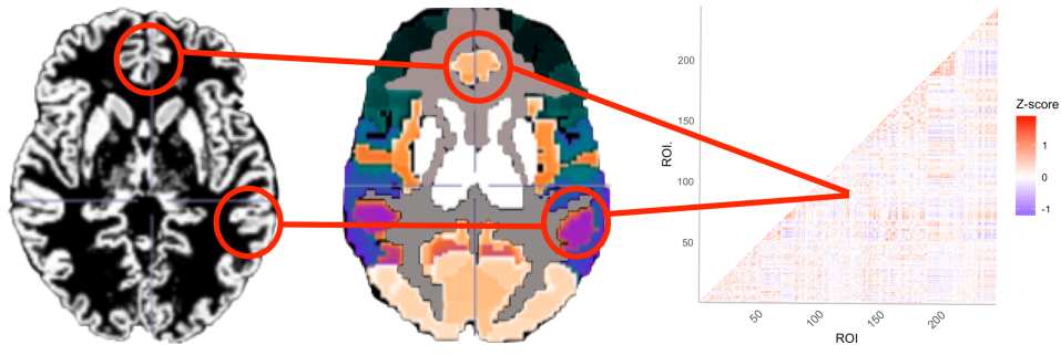
(a) Structural image     (b) Atlas       (c) Network image

Figure 1: Schematic of the multi-object brain imaging data structure for a PPA patient. (a) Structural image encoding voxel-level gray matter (GM) probability, (b) Brainnetome atlas parcellation of the brain into anatomical ROIs, (c) Network image obtained by calculating the pairwise Pearson correlation z-score for the average fMRI signal in each ROI. Red circles and lines connect (a) structural and (c) network information from images via the (b) parcellated atlas. Thus, the atlas provides an organizing hierarchy that links together structural information (GM) at the voxel level with network information indexed by pairs of ROIs (fMRI).

Clinical images and language evaluation: PPA being an infrequently phenotyped ND, imaging data is acquired on $24$ nfvPPA patients during the course of clinical research activity. Data is collected from the following imaging modalities: sMRI derived GM values (Figure 1a) which measures the segmentation probability that a voxel contains neuronal cell bodies (Rajapakse et al., 1997), and task-free resting state fMRI to measure brain activation via neuronal oxygen consumption in subjects at rest. All images are registered to the Montreal Neurological Institute (MNI) template space with voxels parcellated into 245 ROIs using the Brainnetome atlas such that images across modalities and subjects can be directly compared and each voxel is nested in an anatomically defined ROI (Figure 1b) (Fan et al., 2016). The choice of brain atlas is an important decision in the analysis pipeline as it impacts subsequent results and interpretations. Based on our collaborators’ prior work studying language in patients with PPA, the Brainnetome atlas is selected since it provides a granular parcellation needed to model the subtle structural and network dynamics of speech fluency.

For each subject, a ‘brain network’ represented by a symmetric adjacency matrix is obtained from the fMRI image by considering rows and columns of this matrix corresponding to different ROIs and entries corresponding to the z-scores obtained by Fisher Z-transforming the Pearson correlation of the average fMRI data of two ROIs (Figure 1c). We focus our analysis of language loss on speech rate, the number of words spoken per minute, a measure of motor speech via a subject’s articulation rate. This speech rate measure is automatically extracted from recorded speech from the Grandfather passage, a 129-word block of text meant to elicit a comprehensive set of phonemes in English (Ogar et al., 2007), via SALT software (https://www.saltsoftware.com/), a software platform used to automatically extract language features from recorded speech.

Scientific question of interest: Language loss in nfvPPA patients is driven by neurodegeneration in the left inferior frontal region but the dual role of structural damage and brain connectivity in language loss is not well characterized (Mandelli et al., 2016). Findings from the prior clinical studies based on individual image modalities have identified brain networks related to motor speech/fluency (Mandelli et al., 2016). One of our primary goals is to extend the study of motor speech/fluency to consider multi-modal image data spanning the whole brain to better understand how structural and network changes simultaneously impact speech ability. To do so, we apply our proposed multi-modal framework to regress sophisticated multi-modal images, specifically GM maps which capture focal neurodegeneration, and fMRI brain connectivity networks which capture disruptions of brain connectivity, on the speech rate score. The next section describes the novel regression framework to achieve these scientific goals.

3 Bayesian Regression with Multiple Imaging Responses and Speech Rate as a Predictor

This section presents model development and prior formulation, including the hyper-parameter specification.

3.1 Model Framework

For the $i$th subject, let $y_{i}\in\mathbb{R}$ denote the speech rate measure, ${\boldsymbol{x}}_{i}=(x_{i,1},...,x_{i,H})^{\prime}$ represent the biological and demographic variables and ${\boldsymbol{A}}_{i}$ represent the weighted brain network object. We assume that the network of all subjects is defined on a common set of nodes, with elements of ${\boldsymbol{A}}_{i}$ encoding the strength of network connections between different nodes for the $i$-th subject. In particular, the network object ${\boldsymbol{A}}_{i}$ is expressed in the form of a $P\times P$ matrix with the $(p,p^{\prime})$-th entry of the matrix $a_{i,(p,p^{\prime})}$ signifying the strength of association between the $p$th and $p^{\prime}$th node, where $p,p^{\prime}=1,...,P$ and $P$ is the number of network nodes. This paper specifically focuses on networks that contain no self-relationship, i.e., $a_{i,(p,p)}\equiv 0$, and are un-directed ($a_{i,(p,p^{\prime})}=a_{i,(p^{\prime},p)}$). Such assumptions hold for the data application pertaining to Section 2, where ${\boldsymbol{A}}_{i}$ represents the brain connectome network matrix obtained from the fMRI scan, with each node representing a specific brain ROI and edges signifying correlations between fMRI signals in two regions. Let ${\boldsymbol{g}}_{i,1}$,…,${\boldsymbol{g}}_{i,P}$ denote the $V_{1},...,V_{P}$ dimensional structural objects in regions $\mathcal{R}_{1}$,…,$\mathcal{R}_{P}$, respectively. In the context of our data application, they represent volumetric elements (voxels) of the GM image from the $P$ ROIs. The nested structure of voxels within ROIs provides biologically plausible organization and is instrumental for variable selection and computation as detailed in the upcoming methodological development.

For $i=1,\ldots,n$, we assume that the relationship between the speech rate measure $y_{i}$ varies with every network edge and every GM voxel after accounting for the edge and voxel-specific effect of the biological and demographic covariates, and propose a set of conditionally independent generalized linear models for every network edge and GM voxel, given by

$$E[a_{i,(p,p^{\prime})}]=H_{1}^{-1}\Big{(}\sum_{h=1}^{H}\psi_{p,p^{\prime},h}^{a}x_{i,h}+\theta_{p,p^{\prime}}\>y_{i}\Big{)},\>\>E[g_{i,v,p}]=H_{2}^{-1}\Big{(}\sum_{h=1}^{H}\psi_{p,h}^{g}x_{i,h}+\beta_{v,p}\>y_{i}\Big{)},$$ (1)

for $v=1,\ldots,V_{p};\>\>p=1,\ldots,P$, where $H_{1}(\cdot)$ and $H_{2}(\cdot)$ are the link functions, $\theta_{p,p^{\prime}}$ is the $(p,p^{\prime})$th element of the $P\times P$ matrix ${\boldsymbol{\Theta}}$, $\beta_{v,p}$ is the $v$th element of the $V_{p}$ dimensional vector of coefficients ${\boldsymbol{\beta}}_{p}$, $\psi_{p,p^{\prime},h}^{a}$ denotes the effect of $x_{i,h}$ on the edge connecting $p$th and $p^{\prime}$th nodes of the network matrix and $\psi_{p,h}^{g}$ determines the effect of $x_{i,h}$ on the GM image at a voxel within $\mathcal{R}_{p}$. Considering the symmetry and zero diagonal constraints in the network object ${\boldsymbol{A}}_{i}$, we set $\theta_{p,p^{\prime}}=\theta_{p^{\prime},p}$ and $\theta_{p,p}=0$, for all $1\leq p<p^{\prime}\leq P$. Additionally, we assume a bilinear structure for network effects for covariates, given by $\psi_{p,p^{\prime},h}^{a}=\psi_{p,h}^{a}\psi_{p^{\prime},h}^{a}$, to reduce the parameter space while allowing a sufficiently flexible structure to address potential confounding bias in our primary predictor of interest (Von Rosen, 2018). When both sets of responses follow a normal linear model with an identity link function, (1) becomes

$$a_{i,(p,p^{\prime})}=\sum_{h=1}^{H}\psi_{p,h}^{a}\psi_{p^{\prime},h}^{a}x_{i,h}+\theta_{p,p^{\prime}}\>y_{i}+e_{i}^{(p,p^{\prime})},\>\>g_{i,v,p}=\sum_{h=1}^{H}\psi_{p,h}^{g}x_{i,h}+\beta_{v,p}\>y_{i}+w_{i}^{(v,p)},$$ (2)

for $v=1,\ldots,V_{p};\>\>p=1,\ldots,P,$ where $e_{i}^{(p,p^{\prime})}$ and $w_{i}^{(v,p)}$ represent the errors in the two regression models. This article focuses on integrated learning of the mean structure for two sets of models and assumes $e_{i}^{(p,p^{\prime})}\stackrel{{\scriptstyle ind.}}{{\sim}}N(0,\tau_{\theta}^{2})$ (for $1\leq p<p^{\prime}\leq P$) and $w_{i}^{(v,p)}\stackrel{{\scriptstyle ind.}}{{\sim}}N(0,\tau_{\beta}^{2})$ (for $v=1,\ldots,V_{p}$) for simplicity, following the literature on the multivariate linear response regression model (Goh et al., 2017). Consistent with the symmetry and zero diagonal entry in ${\boldsymbol{A}}_{i}$, we assume $e_{i}^{(p,p^{\prime})}=e_{i}^{(p^{\prime},p)}$ and $e_{i}^{(p,p)}=0$. Therefore, stacking over elements of the network matrix and elements of the GM voxels over each region, (2) can be written as

$${\boldsymbol{A}}_{i}=\sum_{h=1}^{H}{\boldsymbol{\Psi}}_{h}^{a}x_{i,h}+{\boldsymbol{\Theta}}\>y_{i}+{\boldsymbol{E}}_{i},\>\>{\boldsymbol{g}}_{i,p}=\sum_{h=1}^{H}{\boldsymbol{1}}_{V_{p}}\psi_{p,h}^{g}x_{i,h}+{\boldsymbol{\beta}}_{p}\>y_{i}+{\boldsymbol{w}}_{i}^{(p)},\>\>p=1,\ldots,P,$$ (3)

where $[{\boldsymbol{\Psi}}_{h}^{a}]_{i,j}=[{\boldsymbol{\psi}}_{h}^{a}({\boldsymbol{\psi}}_{h}^{a})^{\prime}]_{i,j}$ for $i\neq j$, $[{\boldsymbol{\Psi}}_{h}^{a}]_{i,i}=0$, ${\boldsymbol{\psi}}_{h}^{a}=(\psi_{1,h}^{a},...,\psi_{P,h}^{a})^{\prime}$ and ${\boldsymbol{1}}_{V_{p}}$ represents a $V_{p}$-dimensional vector of ones. The error ${\boldsymbol{E}}_{i}\in\mathbb{R}^{P\times P}$ is the symmetric matrix with zero diagonal entries corresponding to the network object and ${\boldsymbol{w}}_{i}^{(p)}$ is the $V_{p}$-dimensional error vector corresponding to the GM image at the $p$th ROI. The key to integrated learning of the multi-modal data lies in the development of an integrated prior structure on ${\boldsymbol{\Theta}}$ and ${\boldsymbol{\beta}}_{p}$’s, as described in the next section.

3.2 Prior Distribution on Multi-Modal Coefficients

Our integrated prior construction on coefficients ${\boldsymbol{\beta}}_{p}$’s and $\{\theta_{p,p^{\prime}}:p<p^{\prime}\}$ for multi-modal predictors is fundamental to exploiting topology of the image objects and cross-information among them by forming principled linkages among images at the ROI level. The prior construction is aimed at: (a) identification of influential ROIs with uncertainty; (b) shrinkage of unimportant voxel coefficients to zero within an influential ROI; and (c) guaranteeing efficient computation of the posterior for the proposed prior. We cast the problem of identifying influential ROIs from the multi-modal images as a high-dimensional variable selection problem and formulate prior distributions on multi-modal object coefficients building upon the existing literature on prior constructions for high-dimensional regression coefficients.

To this end, two classes of prior distributions on coefficients are typically employed in high-dimensional regression literature. The traditional approach is to develop a discrete mixture of prior distributions (George and McCulloch, 1993; Scott and Berger, 2010). These methods enjoy the advantage of inducing exact sparsity for a subset of parameters but may face computational challenges when the number of coefficients is large. As an alternative to this approach, a continuous approximation to the discrete mixture priors (Carvalho et al., 2010) have emerged which induce approximate sparsity in high-dimensional parameters. Such prior distributions can mostly be expressed as global-local scale mixtures of Gaussians (Polson and Scott, 2010), are computationally efficient, and offer an approximation to the operating characteristics of discrete mixture priors.

The direct application of variable selection prior to multi-modal coefficients is unappealing for multiple reasons. First, an ordinary variable selection prior on coefficients ${\boldsymbol{\Theta}}$ and ${\boldsymbol{\beta}}_{p}$’s identifies cells in ${\boldsymbol{A}}_{i}$ and ${\boldsymbol{g}}_{i,p}$ (which in our application refers to the network edges and GM voxels) significantly related to the predictor, rather than identifying influential ROIs. Second, we seek to impose two additional restrictions on the prior construction of ${\boldsymbol{\Theta}}$ and ${\boldsymbol{\beta}}_{p}$ motivated by the neuro-scientific application. First, if at least one of the $p$th and $p^{\prime}$th ROIs is not related to the speech rate, the edge coefficient $\theta_{p,p^{\prime}}$ corresponding to the edge between $p$th and $p^{\prime}$th nodes is unimportant. Second, if the $p$ ROI is deemed uninfluential then all voxels within the $p$th ROI are unrelated to the speech rate, i.e., ${\boldsymbol{\beta}}_{p}={\boldsymbol{0}}$. These restrictions are relevant due to the hierarchical arrangement of voxels and ROIs and are jointly referred to as the hierarchical constraint. Finally, we expect the matrix of coefficients ${\boldsymbol{\Theta}}$ (which itself can be regarded as describing a weighted network) to exhibit transitivity effects, that is, we expect that if the interactions between regions $p$ and $p^{\prime}$ and between regions $p^{\prime}$ and $p^{\prime\prime}$ are both related to the speech rate, the interaction between regions $p$ and $p^{\prime\prime}$ will likely be associated with the speech rate. The property of transitivity reflects the assumption of small-world network structure which is a popular model for neural organization that achieves the simultaneous demands of network integration and segregation (Bassett and Bullmore, 2006) and has been considered in prior studies of PPA (Nigro et al., 2022; Tao et al., 2020). An ordinary variable selection prior on multi-modal coefficients does not necessarily conform to all these requirements.

Let $\xi_{1},...,\xi_{P}$ denote the binary inclusion indicators corresponding to the $P$ ROIs taking values in $\{0,1\}$, with $\xi_{p}=0$ determining no effect of the $p$th ROI on the response from all covariates. In our construction, the network edge coefficient $\theta_{p,p^{\prime}}$ is endowed with a variable selection prior given by

$$\theta_{p,p^{\prime}}|\lambda_{p,p^{\prime}},\tau^{2}_{\theta},\sigma_{\theta},\xi_{p},\xi_{p^{\prime}}\stackrel{{\scriptstyle ind.}}{{\sim}}\xi_{p}\xi_{p^{\prime}}N(0,\tau^{2}_{\theta}\sigma^{2}_{\theta}\lambda_{p,p^{\prime}}^{2})+(1-\xi_{p}\xi_{p^{\prime}})\delta_{0},\>\>p<p^{\prime},$$ (4)

where $\delta_{0}$ corresponds to the Dirac-delta function, $\lambda_{p,p^{\prime}}$ is a local shrinking parameter corresponding to the $(p,p^{\prime})$th edge and $\sigma_{\theta}$ is the global shrinking parameter for the network coefficient. The prior closely mimics the spike-and-slab variable selection structure with an important difference. While an ordinary spike-and-slab prior introduces a binary inclusion indicator corresponding to each variable, (4) enforces $\theta_{p,p^{\prime}}=0$ when either $\xi_{p}=0$ or $\xi_{p^{\prime}}=0$. Such a formulation is sensible from a network perspective as it implies that the edge connecting two network nodes is unrelated to the predictor when at least one of the network nodes is not influential, i.e., it satisfies hierarchical constraint. Additionally, the formulation naturally incorporates transitivity effects in the network coefficient ${\boldsymbol{\Theta}}$. Further, the use of a single binary inclusion indicator to simultaneously determine the influence of ROIs with respect to both structural and network information is informed by prior evidence that structural atrophy and disruptions of functional connectivity can be co-localized in PPA disease progression (Brown et al., 2019) as well as other progressive NDs (Raj et al., 2015). We further assign half-Cauchy distributions on $\sigma_{\theta}\sim C^{+}(0,1)$ and $\lambda_{p,p^{\prime}}\stackrel{{\scriptstyle ind.}}{{\sim}}C^{+}(0,1)$ to complete prior specification on network coefficient. Integrating out $\sigma_{\theta}$ and $\lambda_{p,p^{\prime}}$ in (4), $\theta_{p,p^{\prime}}|\tau^{2}_{\theta},\xi_{p}=1,\xi_{p^{\prime}}=1$ follows the popular horseshoe prior (Carvalho et al., 2010) which offers a flexible prior structure for precise estimation of nonzero network edge coefficients a posteriori.

The GM coefficient $\beta_{v,p}$ in the $p$th ROI is modeled using $\beta_{v,p}=\xi_{p}\gamma_{v,p}$, to ensure all voxel coefficients in the $p$th ROI become unrelated to the predictor if the $p$th ROI is uninfluential (i.e., $\xi_{p}=0$), thus satisfying the hierarchical constraint. To estimate voxel level effects in the $p$th ROI on the predictor, each $\gamma_{v,p}$ is assigned a horseshoe shrinkage prior which takes the following scale-mixture representation,

$$\gamma_{v,p}|\phi_{v,p},\eta_{p}^{2},\tau^{2}_{\beta}\sim N(0,\tau^{2}_{\beta}\eta_{p}^{2}\phi_{v,p}^{2}),\>\>\phi_{v,p}\stackrel{{\scriptstyle i.i.d.}}{{\sim}}C^{+}(0,1),\>\>\eta_{p}\stackrel{{\scriptstyle i.i.d.}}{{\sim}}C^{+}(0,1),$$ (5)

for $v=1,...,V_{p};\>p=1,...,P$. The prior structure (5) induces approximate sparsity in voxel-level GM coefficients $\gamma_{v,p}$ by shrinking the components which are less influential toward zero while retaining the true signals (Polson and Scott, 2010). Finally, the binary inclusion indicators are assigned Bernoulli prior distribution $\xi_{p}\stackrel{{\scriptstyle i.i.d.}}{{\sim}}Ber(\nu)$ with $\nu\sim Beta(a_{\nu},b_{\nu})$ to account for multiplicity correction (Scott and Berger, 2010). Notably, an estimate of the posterior probability of the event $\{\xi_{p}=1\}$ shows the uncertainty in identifying the $p$th ROI to be influential. Thus, $P(\xi_{p}=1|\mbox{Data})$ close to $1$ or $0$ signifies strong evidence in favor of identifying the $p$th ROI to be active or inactive, respectively. The prior specification on multi-modal coefficients is completed by assigning an inverse Gamma $IG(a_{\tau_{\theta}},b_{\tau_{\theta}})$ and $IG(a_{\tau_{\beta}},b_{\tau_{\beta}})$ prior on the error variances $\tau^{2}_{\theta}$ and $\tau^{2}_{\beta}$ respectively. We assign $N(0,1)$ prior distribution on $\psi_{p,h}^{a},\psi_{p,h}^{g}$ for all $p=1,...,P$ and $h=1,...,H$.

Notably, the integrated prior distribution ensures significant feedback from voxel-level inference to ROI-level inference. An ROI is determined to be influential by considering the relevance of all the voxels within that ROI, along with the relevant edges of the network object. This means that multiple weak voxel-level signals within an ROI can collectively identify it as influential, or a strong signal at a single voxel can make the ROI influential. Our method achieves a principled Bayesian balance, weighing the strength of all signals contributing to that ROI. We study these aspects empirically in Section 5. Additionally, detailed inference on $\gamma_{v,p}$ enables voxel-level association between the image and the speech rate measure from our method for influential ROIs. However, we emphasize that the $\gamma_{v,p}$ values are assigned a continuous shrinkage prior, meaning they will not be exactly zero in any MCMC iterations. To determine whether a voxel is significantly related to the cognitive variable, we need to apply post-processing on the MCMC samples of $\gamma_{v,p}$ following the approach described in the literature (Li and Pati, 2017; Guha and Rodriguez, 2021). While we present inference on $\beta_{v,p}$, we do not emphasize voxel identification in the simulation study following the post-processing steps with $\gamma_{v,p}$ due to space constraint, since our main focus is identifying influential ROIs.

4 Posterior Computation

Full conditional distributions for all the parameters are available and mostly correspond to standard families (available in the supplementary file). Thus, posterior computation can proceed through a Markov chain Monte Carlo (MCMC) algorithm. The MCMC sampler is run for $5000$ iterations, with the first $1000$ discarded as burn-in. All simulation scenarios show an average effective sample size of over 3143, indicating fairly uncorrelated post-burn-in MCMC samples.

We have implemented our code in R (without using any C++, Fortran, or Python interface) on a cluster computing environment with three interactive analysis servers, 56 cores each with the Dell PE R820: 4x Intel Xeon Sandy Bridge E5-4640 processor, 16GB RAM, and 1TB SATA hard drive. Different replications of the model are implemented under a parallel architecture by making use of the packages doparallel and foreach within R.

$L$ (suitably thinned) post-convergence MCMC samples $\xi_{p}^{(1)},...,\xi_{P}^{(L)}$ of the binary indicator $\xi_{p}$ are used to empirically assess if the $p$th ROI is significantly associated with the response. In particular, the $p$th ROI $\mathcal{R}_{p}$ is related to the response if $\sum_{l=1}^{L}\xi_{p}^{(l)}/L>t$, for $0<t<1$. The ensuing simulation section computes the $F_{1}$ score for $t=0.5$ to decide which ROIs are influential in predicting the response.

Our computational analysis indicates that the algorithm has a complexity of $\mathcal{O}(n^{3}P(P+V))$, where $V=V_{p}$ denotes the number of voxels per region, assuming each region contains an equal number of voxels. With a limited sample size $n$, $P$ and $V$ are the primary drivers of computational complexity. Figure 2 illustrates the computation time as the number of regions $P$ and voxels per region $V$ vary, with the sample size fixed at $n=25$. The figure demonstrates that the algorithm exhibits linear complexity with respect to $V$ and provides insights into how computation time increases with a growing number of regions $P$ while $V$ remains constant.

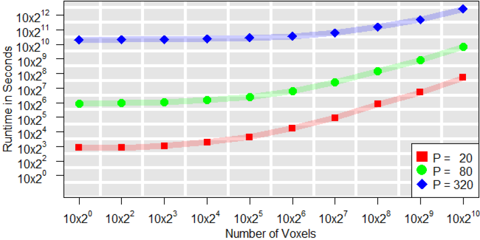
Figure 2: Runtime in seconds for varying number of regions $P$ and number of voxels per region $V$ for fixed $n=25$.

5 Simulation Studies

This section compares our proposed approach, referred to as Bayesian multi-object response regression (BMRR), to that of a few representative frequentist and Bayesian competitors in terms of identifying influential regions and drawing inference on regression coefficients.

5.1 Data Generation

In all our simulations, we assume 3 biological or demographic covariates and a primary covariate of interest. The covariate of interest $y$ is simulated from $N(0,1)$, while we simulate $x_{1}$ form a Bernoulli$(0.5)$, and simulate $x_{2}$ and $x_{3}$ from $N(0,1)$. The coefficients are then simulated as ${\boldsymbol{\psi}}_{p,.t}^{a}\stackrel{{\scriptstyle i.i.d.}}{{\sim}}N({\boldsymbol{0}}_{H},I_{H})$ and ${\boldsymbol{\psi}}_{p,.t}^{g}\stackrel{{\scriptstyle i.i.d.}}{{\sim}}N({\boldsymbol{0}}_{H},I_{H})$ for $p=1,\ldots,P$. We then generate responses ${\boldsymbol{A}}_{i}$ and ${\boldsymbol{g}}_{i,p}$ from model (3) with the true network coefficient ${\boldsymbol{\Theta}}_{t}$ and true structural coefficient ${\boldsymbol{\beta}}_{p,t}$ for the $p$th ROI. The subscript $t$ indicates the true data-generating parameters. In all simulations, we set the sample size to $n=25$ to assess the performance of our approach in a limited sample setting which matches the scenario in our application. We also assume an equal number of voxels per ROI, i.e., $V_{1}=\cdots=V_{P}=V$.

(A1) Non-spatial simulations: Simulating true coefficients ${\boldsymbol{\Theta}}_{t}$ and ${\boldsymbol{\beta}}_{p,t}$. To simulate the true coefficients ${\boldsymbol{\Theta}}_{t}$ and ${\boldsymbol{\beta}}_{p,t}$ without any spatial association between elements of ${\boldsymbol{\beta}}_{p,t}$, we first generate true activation indicators $\{\xi_{p,t}^{\theta}\}_{p=1}^{P}$ for each region corresponding to the network object and $\{\xi_{p,t}^{\beta}\}_{p=1}^{P}$ for each region corresponding to the structural object. The two sets of indicators can impose varying degrees of co-localization between the modalities, as described below.

1. Generate $\kappa_{p,t}\sim Bernoulli(\nu_{t}c_{t})$, where $0\leq\nu_{t}\leq 1$ and $0\leq c_{t}\leq 1$.

2. Generate $\{\xi_{p,t}^{\theta}\}_{p=1}^{P}$ as follows:

   $$\xi_{p,t}^{\theta}=\begin{cases}1&\text{if}\quad\kappa_{p,t}=1\\ \hat{\xi}_{p,t}^{\theta}&\text{if}\quad\kappa_{p,t}=0\end{cases},\>\>\hat{\xi}_{p,t}^{\theta}\sim Bernoulli(\nu_{t}\frac{1-c_{t}}{1-\nu_{t}c_{t}})$$

   where $\hat{\xi}_{p,t}^{\theta}$ indicates activation for region $p$ of the network object independently of the structural object.

3. Generate $\{\xi_{p,t}^{\beta}\}_{p=1}^{P}$ as follows:

   $$\xi_{p,t}^{\beta}=\begin{cases}1&\text{if}\quad\kappa_{p,t}=1\\ \hat{\xi}_{p,t}^{\beta}&\text{if}\quad\kappa_{p,t}=0\end{cases},\>\>\hat{\xi}_{p,t}^{\beta}\sim Bernoulli(\nu_{t}\frac{1-c_{t}}{1-\nu_{t}c_{t}})$$

   where $\hat{\xi}_{p,t}^{\beta}$ indicates activation for region $p$ of the structural object independently of the network object.

4. $p$th region is defined to be influential if either $\xi_{p,t}^{\theta}=1$ or $\xi_{p,t}^{\beta}=1$. Thus, if $\xi_{p,t}$ denotes the true activation of region $\mathcal{R}_{p}$, by definition $\xi_{p,t}=1$ if $\xi^{\theta}_{p,t}=1$ or $\xi^{\beta}_{p,t}=1$.

Note that $c_{t}=1$ implies $\xi_{p,t}=\xi^{\theta}_{p,t}=\xi^{\beta}_{p,t}$. We refer to this case as perfect co-localization. In general, the indicators $\xi^{\theta}_{p,t},\xi^{\beta}_{p,t}$ will be different, with more coincidences as $c_{t}$ is close to $1$, and less coincidences as $c_{t}$ is close to $0$. Importantly, even if $c_{t}=0$, there is a nonzero probability of $\xi_{p,t}=\xi^{\theta}_{p,t}=\xi^{\beta}_{p,t}$ for a region $\mathcal{R}_{p}$. Since $\mathbb{E}[\xi_{p}^{\theta}]=\mathbb{E}[\xi_{p}^{\beta}]=\nu_{t}$, $(1-\nu_{t})$ controls the probability of a region not being “influential”. It is known as the node sparsity parameter.

For each sparsity level and co-localization degree, the coefficient corresponding to the edge connecting the $p$-th and $p^{\prime}$-th region is drawn from the following mixture distribution,

$$\theta_{(p,p^{\prime}),t}|\xi^{\theta}_{p,t},\xi^{\theta}_{p^{\prime},t}\sim\xi_{p,t}^{\theta}\xi_{p^{\prime},t}^{\theta}N(\mu_{\theta,(p,p^{\prime})},\sigma_{\theta}^{2})+(1-\xi_{p,t}^{\theta}\xi_{p^{\prime},t}^{\theta})\delta_{0},\>\>\>\theta_{(p,p^{\prime}),t}=\theta_{(p^{\prime},p),t};.$$ (6)

(6) ensures that any edge connecting to the $p$-th region in the network response is unrelated to the predictor if the $p$-th region is un-influential, i.e., $\xi^{\theta}_{p,t}=0\Rightarrow\theta_{(p,p^{\prime}),t}=0$ for all $p^{\prime}\in\{1,..,P\}$. Similarly, corresponding to each un-influential region $\mathcal{R}_{p}$, i.e., when $\xi^{\beta}_{p,t}=0$, the $V\times 1$ dimensional GM coefficient ${\boldsymbol{\beta}}_{p,t}$ is set at ${\boldsymbol{0}}$. When $\xi^{\beta}_{p,t}=1$, i.e., the $p$-th region is influential, we randomly choose $\upsilon_{t}$ proportion of cell coefficients in the $p$-th region to be nonzero and the rest are set at zero. Thus $\upsilon_{t}$ is the density of activated voxels within a region. The nonzero coefficients within ${\boldsymbol{\beta}}_{p,t}$ are simulated from $N(\mu_{\beta,(v,p)},\sigma_{\beta}^{2})$, where the values of $\mu_{\theta,(p,p^{\prime})}$ and $\mu_{\beta,(v,p)}$ are drawn from $Unif(0.25,1)$. We fix $\sigma_{\theta}^{2}=1$, $\sigma_{\beta}^{2}=1$. We control the signal-to-noise ratio by changing the error variances $\tau_{t,\theta}^{2}$ and $\tau_{t,\beta}^{2}$.

(A2) Spatial simulations: Simulating true coefficients ${\boldsymbol{\Theta}}_{t}$ and ${\boldsymbol{\beta}}_{p,t}$. We also consider simulation scenarios where structural coefficients are spatially indexed, i.e., $\beta_{v,p}=\beta({\boldsymbol{s}}_{v,p})$, with ${\boldsymbol{s}}_{v,p}$ representing the spatial location of the $v$th voxel in the $\mathcal{R}_{p}$. This simulation setting assumes perfect co-localization, i.e., $\xi_{p,t}=\xi_{p,t}^{\theta}=\xi_{p,t}^{\beta}$. The network edge coefficient $\theta_{(p,p^{\prime}),t}$ is simulated following (6). When $\xi_{p,t}=1$, we randomly choose $\upsilon_{t}$ proportion of voxel coefficients in $\mathcal{R}_{p}$ to be nonzero, and the rest are set at zero. the nonzero coefficient $\beta({\boldsymbol{s}}_{v,p})$ is simulated from a Gaussian process with mean 1 and a covariance function given by the Matérn Kernel: $cor(\beta({\boldsymbol{s}}_{v,p}),\beta({\boldsymbol{s}}_{v^{\prime},p}))=K(d|\rho,\nu)=\frac{2^{1-\nu}}{\Gamma(\nu)}\left((2\nu)^{1/2}\frac{d}{\rho}\right)^{\nu}K_{\nu}\left((2\nu)^{1/2}\frac{d}{\rho}\right),$ where $d=||{\boldsymbol{s}}_{v,p}-{\boldsymbol{s}}_{v^{\prime},p}||$ and $K_{\nu}$ is the modified Bessel function of order $\nu$. We set $\nu=2$ to ensure a fairly smooth spatial surface and $\rho=1$ for a reasonable range of spatial dependence.

We simulate data under two different node sparsity parameters, $(1-\nu_{t})=0.85,0.70$. Finally, a different number of ROIs and different numbers of voxels within an ROI are considered. Specifically, we consider two cases, (a) $P=20$ and $V=10$, and (b) $P=100$ and $V=50$. Cases (a) and (b) are referred to as the “small dimensional example” and “high dimensional example.” In both these cases we have approximately similar number of parameters to estimate from the network and the structural coefficients. We also vary the signal-to-noise ratio at values $0.25,0.5,1,2,4$. All simulation scenarios are summarized in Table 1. Notably, the fitted model in Section 3 assumes co-localization. Hence, simulations under nonzero $c_{t}$ and spatial correlation between GM coefficients will allow us to assess the performance of BMRR under more realistic scenarios with model mis-specifications.

Table 1: Simulation scenarios by varying degree of co-localization ($c_{t}$), node sparsity parameter ($1-\nu_{t}$), signal-to-noise ratio, number of ROIs and number of voxels per ROI, and the density of activated voxels per region ($\upsilon_{t}$).

		node sparsity $(1-\nu_{t})=$ 0.85			node sparsity $(1-\nu_{t})=$ 0.70
	$SNR$	$c_{t}=1$	$c_{t}=0.5$	$c_{t}=0$	$c_{t}=1$	$c_{t}=0.5$	$c_{t}=0$
Low	$4$	$\upsilon_{t}=(0.05,..,1)$	$\upsilon_{t}=(0.05,..,1)$	$\upsilon_{t}=(0.05,..,1)$	$\upsilon_{t}=(0.05,..,1)$	$\upsilon_{t}=(0.05,..,1)$	$\upsilon_{t}=(0.05,..,1)$
Dim.	$2$	$\upsilon_{t}=(0.05,..,1)$	$\upsilon_{t}=(0.05,..,1)$	$\upsilon_{t}=(0.05,..,1)$	$\upsilon_{t}=(0.05,..,1)$	$\upsilon_{t}=(0.05,..,1)$	$\upsilon_{t}=(0.05,..,1)$
	$1$	$\upsilon_{t}=(0.05,..,1)$	$\upsilon_{t}=(0.05,..,1)$	$\upsilon_{t}=(0.05,..,1)$	$\upsilon_{t}=(0.05,..,1)$	$\upsilon_{t}=(0.05,..,1)$	$\upsilon_{t}=(0.05,..,1)$
	$0.5$	$\upsilon_{t}=(0.05,..,1)$	$\upsilon_{t}=(0.05,..,1)$	$\upsilon_{t}=(0.05,..,1)$	$\upsilon_{t}=(0.05,..,1)$	$\upsilon_{t}=(0.05,..,1)$	$\upsilon_{t}=(0.05,..,1)$
	$0.25$	$\upsilon_{t}=(0.05,..,1)$	$\upsilon_{t}=(0.05,..,1)$	$\upsilon_{t}=(0.05,..,1)$	$\upsilon_{t}=(0.05,..,1)$	$\upsilon_{t}=(0.05,..,1)$	$\upsilon_{t}=(0.05,..,1)$
High	$4$	$\upsilon_{t}=(0.05,..,1)$	$\upsilon_{t}=(0.05,..,1)$	$\upsilon_{t}=(0.05,..,1)$	$\upsilon_{t}=(0.05,..,1)$	$\upsilon_{t}=(0.05,..,1)$	$\upsilon_{t}=(0.05,..,1)$
Dim.	$2$	$\upsilon_{t}=(0.05,..,1)$	$\upsilon_{t}=(0.05,..,1)$	$\upsilon_{t}=(0.05,..,1)$	$\upsilon_{t}=(0.05,..,1)$	$\upsilon_{t}=(0.05,..,1)$	$\upsilon_{t}=(0.05,..,1)$
	$1$	$\upsilon_{t}=(0.05,..,1)$	$\upsilon_{t}=(0.05,..,1)$	$\upsilon_{t}=(0.05,..,1)$	$\upsilon_{t}=(0.05,..,1)$	$\upsilon_{t}=(0.05,..,1)$	$\upsilon_{t}=(0.05,..,1)$
	$0.5$	$\upsilon_{t}=(0.05,..,1)$	$\upsilon_{t}=(0.05,..,1)$	$\upsilon_{t}=(0.05,..,1)$	$\upsilon_{t}=(0.05,..,1)$	$\upsilon_{t}=(0.05,..,1)$	$\upsilon_{t}=(0.05,..,1)$
	$0.25$	$\upsilon_{t}=(0.05,..,1)$	$\upsilon_{t}=(0.05,..,1)$	$\upsilon_{t}=(0.05,..,1)$	$\upsilon_{t}=(0.05,..,1)$	$\upsilon_{t}=(0.05,..,1)$	$\upsilon_{t}=(0.05,..,1)$

5.2 Competitors and Metrics of Comparison

The simulated data will be used to assess the performance of: (A) identifying influential regions; (B) estimating the true network coefficient ${\boldsymbol{\Theta}}_{t}$ and structural coefficients ${\boldsymbol{\beta}}_{1,t},...,{\boldsymbol{\beta}}_{P,t}$; and (C) quantifying uncertainty in the point estimation of network and structural coefficients. We construct a series of competitors of BMRR to assess (A)-(C) as described below.

5.2.1 Frequentist competitors

As frequentist competitors, we implement popularly used mass univariate analysis (MUA). In this approach each network edge and each cell of the structural image is regressed on the predictor of interest, along with biological and demographic covariates via multiple linear regression with a bi-linear structure on the coefficients to obtain p-values corresponding to the point estimates of $\theta_{p,p^{\prime}}$ and $\beta_{v,p}$, denoted by p-value($\hat{\theta}_{p,p^{\prime}}$) and p-value($\hat{\beta}_{v,p}$), respectively, for $v=1,...,V_{p}$ and $p=1,...,P$. These p-values will be compared to a threshold to declare if a region is influential, after accounting for the multiple comparison issues by controlling the False Discovery Rate (FDR) (Genovese et al., 2002). Specifically, MUA orders p-value($\hat{\beta}_{v,p}$) and p-value($\hat{\theta}_{p,p^{\prime}}$) for all $v=1,...,V_{p}$, $1\leq p<p^{\prime}\leq P$ in ascending order. Let $\text{p-value}_{(1)},...,$
$\text{p-value}_{\left(\frac{P(P-1)}{2}+\sum_{p=1}^{P}V_{p}\right)}$ be the ordered p-values and let $i^{*}$ be the largest index such that $\text{p-value}_{(i^{*})}\leq\frac{i^{*}\alpha_{0}}{\frac{P(P-1)}{2}+\sum_{p=1}^{P}V_{p}}$. A region $p$ is identified as influential if $\text{p-value}(\hat{\theta}_{p,p^{\prime}})\leq\text{p-value}_{(i^{*})}$ for at least one $p^{\prime}\neq p$, or $\text{p-value}(\hat{\beta}_{v,p})\leq\text{p-value}_{(i^{*})}$ for at least one $v\in\{1,...,V_{p}\}$. We set $\alpha_{0}=0.05$ throughout this discussion. We also implement tensor response regression (Li and Zhang, 2017) where both objects are viewed as 2D tensors in the simulation. Parsimonious tensor response regression (TRR) is applied to each object separately with the simulated speech rate measure ${y_{i}}$ and the biological and demographic covariates ${\boldsymbol{x}}_{i}$ as independent variables using the R package TRES. A region is considered influential by TRR if either an edge connected to that region or a voxel in that region is influential.

5.2.2 Bayesian competitors

We construct a few Bayesian competitors to compare single modal analysis and joint analysis of modalities without integrating information between objects, with the integrative analysis performed by BMRR. These competitors include:
(a) fitting only the Bayesian network on scalar regression (i.e., the first equation in (3)), referred to as the network response regression (NRR); (b) fitting only the Bayesian structural images on scalar regression (i.e., the second equation in (3), referred to as the structural response regression (SRR); and (c) fitting both of them jointly without integrating them through shared parameters, referred to as the joint regression (JR). For NRR, a region is identified as influential if at least one edge connecting to that region is influential. In SRR, a region is deemed influential if it contains at least one influential voxel. For JR, a region is identified as influential if any voxel in that region or any edge connected to that region is influential.

We implement two additional Bayesian competitors, both capturing joint effects of all network edges and cells of the structural images on the predictor, but do not acknowledge the network topology or the connection between the topology of two sets of objects through the hierarchical constraint. The first Bayesian competitor, referred to as the Spike & Slab, applies an ordinary spike & slab prior (George and McCulloch, 1993) on each $\theta_{p,p^{\prime}}$ and $\beta_{v,p}$. A voxel or an edge will be identified as influential if the posterior probability that the corresponding coefficient equals zero exceeds $0.5$ (Barbieri and Berger, 2004). We also implement a Horseshoe shrinkage prior (Carvalho et al., 2010) on each $\theta_{p,p^{\prime}}$ and $\beta_{v,p}$. Since the Horseshoe prior does not result in exact zeros for the post-burn-in iterates of coefficients, we perform a post-processing approach following Li and Pati (2017) to determine which voxel coefficients and network edges are related to the predictor. For both Spike & Slab and Horseshoe competitors, an ROI $\mathcal{R}_{p}$ is identified as influential if at least a network edge connecting to that ROI or at least on voxel coefficient within the ROI is nonzero.

5.2.3 Metrics of comparison

We will present the $F_{1}$ score computed from the True Positive Rate (TPR) and the True Negative Rate (TNR) for correctly identifying important regions. The point estimation of every competitor is assessed using mean squared errors (MSE) of estimating the network coefficient ${\boldsymbol{\Theta}}_{t}$ and the structural coefficients ${\boldsymbol{\beta}}_{1,t},...,{\boldsymbol{\beta}}_{P,t}$. Since both the fitted ${\boldsymbol{\Theta}}$ and ${\boldsymbol{\Theta}}_{t}$ are symmetric with zero diagonals, the MSE for both sets of coefficients jointly is given by $[\sum_{p<p^{\prime}}(\theta_{p,p^{\prime},t}-\widehat{\theta}_{p,p^{\prime}})^{2}+\sum_{p=1}^{P}||{\boldsymbol{\beta}}_{p,t}-\widehat{{\boldsymbol{\beta}}}_{p}||^{2}]/(P(P-1)/2+VP)$. The point estimates are taken to be the posterior median for the Bayesian competitors. For Bayesian competitors, we evaluate the length and coverage of 95% credible intervals averaged across coefficients in ${\boldsymbol{\Theta}}$ and present them for all cases. Similar quantities for ${\boldsymbol{\beta}}_{p}$’s are also presented. All results presented over $500$ simulated datasets.

5.3 Results

Figure 3 presents the $F_{1}$ score for BMRR region identification under each of our simulation scenarios in Table 1. As the voxel density parameter $\upsilon_{t}$ approaches 0, indicating high voxel-sparsity, region identification suffers. Similarly, BMRR’s performance deteriorates with lower SNR. However, for the same $\upsilon_{t}$ and SNR, BMRR performs better in high-dimensional cases than in low-dimensional cases. Additionally, for the same levels of $\upsilon_{t}$, SNR, and $(V,P)$, BMRR performs better with a higher degree of co-localization, since it induces co-localization in its modeling framework. Finally, we observe that the smoothly varying spatial correlation structure over the voxels of the structural images does not significantly impact BMRR’s performance in terms of region identification.

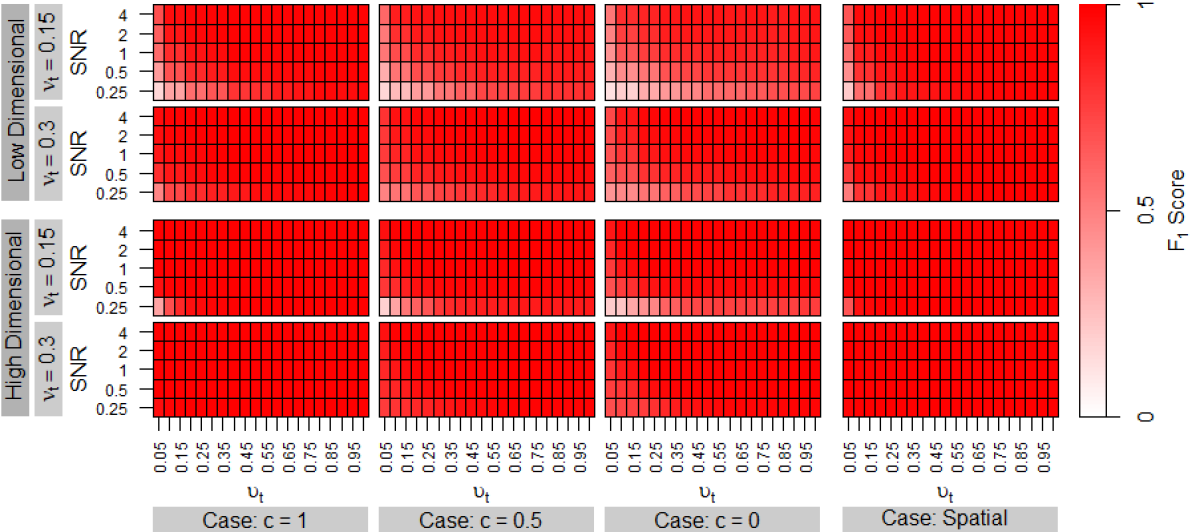
Figure 3: $F_{1}$ score for BMRR under simulation scenarios outlined in Table 1.

Figure 4 shows boxplots of $F_{1}$ scores for structured Bayesian regressions BMRR, NRR, SRR, and JR under various simulation scenarios. Due to space constraints, we present results for moderate and low SNR values of $1$ and $0.5$, and voxel density parameter $\upsilon_{t}=0.2$ and $0.4$. It is evident that the integrated version, BMRR, consistently outperforms using either or both objects independently. While using both objects in JR improves performance compared to using only one image in NRR or SRR, the improvement is not as significant as when using the integrated BMRR approach. Both BMRR and JR show marginal performance improvements with increasing SNR, increasing co-localization degree, and in high-dimensional settings. In contrast, the improvement is significant for NRR and SRR in the high-dimensional setting. All competitors show better performance with increasing voxel density as well as with decreasing node sparsity within a limit. Additionally, the $F_{1}$ scores do not show any significant perturbation with spatial association between voxels of the structural image.

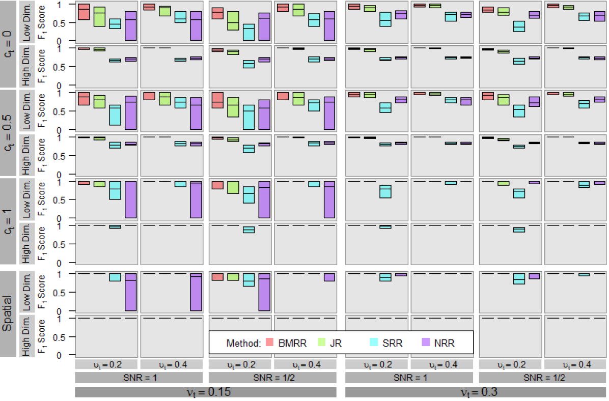
Figure 4: $F_{1}$ score for different simulation scenarios for BMRR integrating the objects, using both objects without integration (JR), only the structural object (SRR), and only the network object (NRR).

Our focus now lies on the performance of BMRR compared to other competitors excluding the Bayesian structured regressions. Due to space restrictions, we only consider representative simulation cases where SNR is $1$, node sparsity $(1-\nu_{t})=0.7$, and voxel density $\upsilon_{t}=0.4$. Results for other simulation cases lead to similar conclusions.

According to Figure 5, BMRR outperforms every competitor in every scenario in terms of $F_{1}$ score. While Spike & Slab, Horseshoe, and MUA show average $F_{1}$ scores close to 1 as the co-localization degree increases, their scores exhibit wide variability over replications, as demonstrated by the large interquartile ranges. TRR performs poorly across all scenarios. BMRR also outperforms other competitors in terms of estimating network and structural coefficients, as evidenced by the smallest MSE values under all scenarios. Spike & Slab and Horseshoe perform similarly to each other, while MUA and TRR show the poorest performance. Notably, the performance of all competitors remains largely unchanged between spatial and non-spatial scenarios with perfect co-localization. For uncertainty quantification, we observe that all methods offer nominal or slight over-coverage, except for TRR, which shows severe under-coverage. Additionally, BMRR provides narrower 95% credible intervals than its competitors under all scenarios, with the exception of Spike & Slab, which marginally outperforms BMRR in low-dimensional cases.

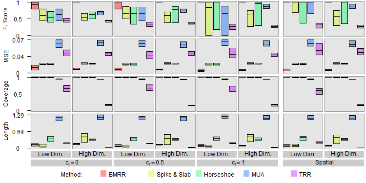
Figure 5: $F_{1}$ score, MSE, and $95\%$ interval coverage and length for BMRR and frequentist and Bayesian competitors. The interquartile range and median across simulations are presented.

6 Application to the multi-modal PPA data

6.1 Data structure and methods

In our motivating study, sMRI GM, resting state fMRI connectivity images, and speech rates (described in Section 2) were collected at the University of California, San Francisco Memory and Aging Center on 24 subjects with nfvPPA (10 males and 14 females) aged between 57 and 81 years (68.9 years old on average). sMRI GM maps were preprocessed as in Canu et al. (2020) and fMRI network images were processed as in Montembeault et al. (2023). We adjust our analysis for biological sex, age, and cognitive function measured via the mini-mental state examination (MMSE) scale as a measure of dementia severity as in García et al. (2022).

The sMRI GM segmentation probabilities and fMRI Pearson correlations were transformed via inverse normal cumulative distribution function and Fisher Z-transformation, respectively, to produce z-scores that satisfy assumptions of the error distribution. The sMRI GM and fMRI network connectivity images were each mean centered for a fixed voxel and edge across subjects, respectively. The biological sex indicator is encoded as 1 for male and 0 for female. The covariates MMSE and age are mean-centered. Finally, the speech rate predictor variable has been normalized to have a mean of zero and a standard deviation of one. We set out to compare the inferential outcomes from BMRR to the best-performing competitors in the simulations, i.e., MUA, Horseshoe, JR, and TRR. Unfortunately, TRES package sends an error message while implementing TRR, which precludes its usage as a competitor.

6.2 Data analysis results

We present the results from our application of the proposed BMRR to the multi-modal PPA imaging data. In total, 46 out of 245 ROIs have a posterior probability $P(\xi_{p}=1|\mbox{Data})>0.5$ of being associated with speech rate in the multi-modal data. The set of influential ROIs and their posterior probability of being influential (which is a measure of uncertainty) are recorded in Table 2. In general, the ROIs lie in areas of the brain previously associated with language, motor speech, and neurodegeneration in PPA, specifically the frontal lobe including the superior frontal gyrus (SFG) (Landin-Romero et al., 2021), the middle frontal gyrus (MFG) (Landin-Romero et al., 2021), the inferior frontal gyrus (IFG) (García et al., 2022), the inferior parietal lobe (IPL) (Bzdok et al., 2016), the superior parietal lobe (SPL) (Alahmadi, 2021), and the basal ganglia (BG) (Montembeault et al., 2018) (see Fan et al. (2016) for Brainnetome atlas ROI naming conventions). The 46 ROIs display a bilateral distribution which is consistent with previous findings that indicate that articulation can be impacted by disruptions in the motor speech network in either the left or right hemisphere of the motor speech network (Landin-Romero et al., 2021).

Figure 6 displays horizontal slices (higher c coordinate refers to the top of the brain) of the GM coefficient map organized by ROI where the colored shading indicates the magnitude and direction of association of the speech rate with z-score GM segmentation probability. Due to the hierarchical nature of the BMRR model, the distribution of influential GM voxels (as captured by their associated coefficients) is determined by the ROI selection and thus reflects the distribution of the selected 46 ROIs discussed above, with concentrations in the SFG, MFG, IFG, IPL, SPL, and BG in a bilateral distribution. The GM coefficient maps provide an additional level of granularity by characterizing the association between the speech rate and GM probability at the voxel level as well as the sparsity of the signal which varies by ROI. Overall, speech rate is positively associated with increases in voxel level GM in the frontal gyrus which affirms that a decrease in GM in these regions is correlated with lower articulation rates (Landin-Romero et al., 2021; García et al., 2022). However, there is heterogeneity in the voxel level signal both within and across ROIs with a substantial number of voxels displaying a negative association of GM with speech rate particularly in the parietal lobe. The effect sizes range from -1.4 to 1.4 across voxels which indicates that a standard deviation shift in speech rate (25 words/minute) can produce a change in z-score GM segmentation probability from between -1.4 and 1.4. These results reveal a dynamic portrait of how GM and neurodegeneration are associated with motor speech and highlight heterogeneity in the direction of the association as well as varying levels of sparsity in influential voxels across ROIs, insights that are missed when data is pooled at the ROI level.

Figure 7 displays the ROI level network coefficient maps organized by anatomical brain region where the top and bottom half of each anatomical region indicated by a horizontal dash corresponds to the left hemisphere and right hemispheres, respectively. The colored shading indicates the magnitude and direction of association of the speech rate with resting state functional connectivity (measured as the Fisher Z-transformed pairwise Pearson correlation). The network edges associated with the speech rate are sparse and there is almost always a positive association between functional connectivity and speech rate. There is a high degree of bilateral functional connectivity associated with speech rate both among and between the SFG, MFG, and IFG brain regions in the frontal lobe. Connections extend outside the frontal lobe and higher speech rates are also associated with higher functional connectivity between the frontal lobe and the parietal lobe which has been indicated in higher-order language processing (Coslett and Schwartz, 2018), including the SPL, IPL, and the precuneus (PCun). The effect sizes range from -0.01 to 0.24 across network edges which indicates that a standard deviation shift in speech rate (25 words/minute) can produce a change in Fisher Z-transformed correlation between -0.01 to 0.24. Supplementary Figures 1-3 show the GM coefficient maps for the covariates gender, age, and MMSE, and Figures 4-6 show the same for network coefficient maps and are interpreted in a similar manner to the speech rate coefficient maps, albeit without the hierarchical regularization priors.

We compare the results from the application of the proposed BMRR to the MUA. Figures 7-8 in the supplementary file show that very few GM voxels and network edges are selected, providing us with very few signals for analysis in MUA. We also contrast BMRR with Horseshoe and JR in terms of the Posterior Predictive Loss Criterion (PPLC) that shows the fit of the three competing models. The results presented in Table 3 show better model fit by BMRR than JR, indicating the advantages of integrating information from objects. Given that the coefficients for the speech rate measure are not very large, BMRR has only a modest advantage over Horseshoe in model fitting statistics. However, Horseshoe proves extremely unreliable in identifying influential ROIs, as it marks all ROIs as influential, rendering the results scientifically uninterpretable. Overall, BMRR develops novel insights on the neuro-degeneration pathway for PPA and outperforms competitors due to accounting for science-driven constraints in the prior structure for coefficients.

Table 2: Influential ROIs identified by BMRR in the PPA data analysis along with their posterior probabilities of being influential. See Fan et al. (2016) for Brainnetome atlas ROI naming conventions.

ROI	Prob.	ROI	Prob.	ROI	Prob.	ROI	Prob.
BG_L_6_1	0.930	IPL_L_6_2	0.722	MFG_R_7_3	0.882	SFG_L_7_4	1.000
BG_L_6_2	1.000	IPL_L_6_3	0.800	MFG_R_7_4	0.586	SFG_L_7_7	0.858
BG_L_6_4	1.000	IPL_L_6_5	1.000	MFG_R_7_5	1.000	SFG_R_7_2	0.784
BG_L_6_5	0.820	IPL_R_6_5	1.000	MFG_R_7_6	0.800	SFG_R_7_3	0.908
BG_R_6_1	0.822	MFG_L_7_1	0.964	MFG_R_7_7	1.000	SFG_R_7_4	0.948
BG_R_6_2	1.000	MFG_L_7_2	0.596	MTG_L_4_1	0.650	SPL_L_5_2	1.000
BG_R_6_4	1.000	MFG_L_7_3	1.000	PCun_R_4_1	1.000	SPL_L_5_5	1.000
CG_R_7_3	0.986	MFG_L_7_4	1.000	PCun_R_4_2	1.000	SPL_R_5_2	0.952
CG_R_7_5	1.000	MFG_L_7_5	0.526	PhG_L_6_4	1.000	SPL_R_5_3	0.766
IFG_L_6_3	1.000	MFG_L_7_6	1.000	PhG_R_6_5	0.726	Tha_L_8_2	1.000
IFG_R_6_2	1.000	MFG_R_7_1	0.876	PoG_L_4_3	1.000
IFG_R_6_3	0.952	MFG_R_7_2	0.910	PrG_L_6_2	1.000

In our empirical analysis, we set the hyper-parameter values as $a_{\nu}=b_{\nu}=1=a_{\tau_{\theta}}=b_{\tau_{\theta}}=a_{\tau_{\beta}}=b_{\tau_{\beta}}=1$. To assess the sensitivity to the choice of hyper-parameters, data analysis is conducted with different combinations of hyper-parameters. Specifically, we vary $a_{\nu}=b_{\nu}$ at values $0.1,1,10$. For each such choice, we vary $a_{\tau_{\theta}}=b_{\tau_{\theta}}=a_{\tau_{\beta}}=b_{\tau_{\beta}}$ at values $0.1,1,10$. For each hyper-parameter combination, MSPE, coverage of the 95% predictive interval, and the length of the 95% predictive intervals averaged over all image voxels and network edges are shown. We also compute the Adjusted Rand Index (ARI) between the partitions of influential and uninfluential node indices obtained from a specific combination of hyper-parameters and from the choice $a_{\nu}=b_{\nu}=1$ and $a_{\tau_{\theta}}=b_{\tau_{\theta}}=a_{\tau_{\beta}}=b_{\tau_{\beta}}=1$. All these metrics in Table 4 indicate that BMRR is largely insensitive to the choice of hyper-parameters.

Table 3: Weighted Posterior Predictive Loss Criterion (PPLC) as in as in Gelfand and Ghosh (1998) for values of for BMRR, using the non-integrated version of BMRR (JR) and Horseshoe. $PPLC=G+P$, where G is associated with goodness of fit and P is associated with a penalty related to model complexity.

Method	$G$	$P$	PPLC
BMRR	2094.40	54490.50	56584.90
JR	2243.31	54480.63	56723.94
Horseshoe	2316.32	54481.55	56797.87

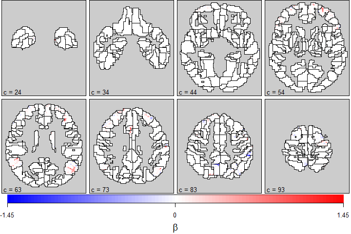
Figure 6: Point estimates (median) of the regression coefficients for gray matter segmentation probability z-scores for selected voxels across horizontal slices using BMRR with speech rate as predictor.

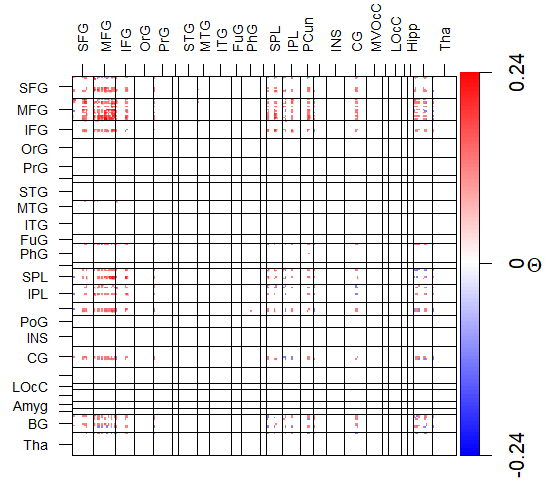
Figure 7: Point estimates (median) of the regression coefficients for Network Matrix z-scores using BMRR with speech rate as predictor. Each cell displays the ROI level network coefficient maps organized by anatomical brain region where the top and bottom half of each anatomical region indicated by a horizontal dash corresponds to the left hemisphere and right hemispheres, respectively.

Table 4:  Sensitivity analysis for the hyper-parameters. Performance measures with different combinations of hyper-parameters, and ARI and proportion of matches of regions selected and unselected with respect to the hyper-parameter combination $a_{\nu}=b_{\nu}=1=a_{\tau_{\theta}}=b_{\tau_{\theta}}=a_{\tau_{\beta}}=b_{\tau_{\beta}}=1$.

	$a_{\nu}=b_{\nu}=0.1$			$a_{\nu}=b_{\nu}=1$			$a_{\nu}=b_{\nu}=10$
$a_{\tau_{\theta}}=b_{\tau_{\theta}}=a_{\tau_{\beta}}=b_{\tau_{\beta}}=$	0.1	1	10	0.1	1	10	0.1	1	10
ARI	1	1	1	1	1	1	1	1	0.981
Proportion of Matches	1	1	1	1	1	1	1	1	0.996
MSPE	0.823	0.819	0.825	0.825	0.823	0.825	0.824	0.821	0.826
Interval Coverage	0.914	0.918	0.906	0.908	0.908	0.906	0.912	0.914	0.908
Interval Length	0.015	0.014	0.014	0.015	0.014	0.014	0.015	0.015	0.014

7 Conclusion and Future Work

Motivated by multi-modal imaging applications constituting the structural and functional imaging data on patients with PPA, this article develops a regression approach with structural and network-valued objects on a scalar predictor. A novel prior structure is developed jointly on coefficients corresponding to different objects which can simultaneously exploit object characteristics and the linked information between the objects to draw inference on network nodes significantly related to the scalar predictor with uncertainty. The proposed approach is arguably the first statistical multi-modal response regression approach that allows for the flexibility of drawing inference at the ROI level and the voxel level simultaneously and is equipped with identifying brain regions significantly related to the speech rate measuring neuro-degeneration due to PPA with uncertainty. The analysis of PPA data leads to an important understanding of neuro-degeneration patterns associated with PPA.

The study has some important limitations and considerations. Our results leverage the organizing hierarchy of the Brainnetome atlas and its associated ROIs to connect structural and network information. Thus, conclusions might differ had an alternate brain atlas been used. While sensitivity analyses utilizing different brain atlas could be conducted, we emphasize that our proposed technique and its application to the PPA data is based on strong prior neuroanatomical knowledge that the Brainnetome atlas and subsequent parcellation is appropriate for the clinical question of interest. In settings where investigators are unsure of the appropriate atlas, greater emphasis should be placed on assessing the sensitivity of results to the selection of alternate parcellations. In addition, PPA being an infrequently studied disease, our results are based on a modest sample size which requires cautious interpretation of results as discussed in Section 2. As an immediate future work, we will extend our approach to incorporate the spatial correlation in the GM image.

References

- Alahmadi (2021) Alahmadi, A. A. S. (2021). Investigating the sub-regions of the superior parietal cortex using functional magnetic resonance imaging connectivity. Insights Imaging, 12(1), 47.
- Barbieri and Berger (2004) Barbieri, M. M. and Berger, J. O. (2004). Optimal predictive model selection. The annals of statistics, 32(3), 870–897.
- Bassett and Bullmore (2006) Bassett, D. S. and Bullmore, E. (2006). Small-world brain networks. Neuroscientist, 12(6), 512–523.
- Battistella et al. (2020) Battistella, G., Borghesani, V., Henry, M., Shwe, W., Lauricella, M., Miller, Z., Deleon, J., Miller, B. L., Dronkers, N., Brambati, S. M., Seeley, W. W., Mandelli, M. L., and Gorno-Tempini, M. L. (2020). Task-Free functional language networks: Reproducibility and clinical application. J. Neurosci., 40(6), 1311–1320.
- Brown et al. (2019) Brown, J. A., Deng, J., Neuhaus, J., Sible, I. J., Sias, A. C., Lee, S. E., Kornak, J., Marx, G. A., Karydas, A. M., Spina, S., Grinberg, L. T., Coppola, G., Geschwind, D. H., Kramer, J. H., Gorno-Tempini, M. L., Miller, B. L., Rosen, H. J., and Seeley, W. W. (2019). Patient-tailored, connectivity-based forecasts of spreading brain atrophy. Neuron, 104(5), 856–868.
- Bzdok et al. (2016) Bzdok, D., Hartwigsen, G., Reid, A., Laird, A. R., Fox, P. T., and Eickhoff, S. B. (2016). Left inferior parietal lobe engagement in social cognition and language. Neurosci. Biobehav. Rev., 68, 319–334.
- Calhoun and Sui (2016) Calhoun, V. D. and Sui, J. (2016). Multimodal fusion of brain imaging data: A key to finding the missing link (s) in complex mental illness. Biological psychiatry: cognitive neuroscience and neuroimaging, 1(3), 230–244.
- Canu et al. (2020) Canu, E., Agosta, F., Battistella, G., Spinelli, E. G., DeLeon, J., Welch, A. E., Mandelli, M. L., Hubbard, H. I., Moro, A., Magnani, G., Cappa, S. F., Miller, B. L., Filippi, M., and Gorno-Tempini, M. L. (2020). Speech production differences in english and italian speakers with nonfluent variant PPA. Neurology, 94(10), e1062–e1072.
- Carvalho et al. (2010) Carvalho, C. M., Polson, N. G., and Scott, J. G. (2010). The horseshoe estimator for sparse signals. Biometrika, 97(2), 465–480.
- Chen et al. (2013) Chen, J., Bushman, F. D., Lewis, J. D., Wu, G. D., and Li, H. (2013). Structure-constrained sparse canonical correlation analysis with an application to microbiome data analysis. Biostatistics (Oxford, England), 14(2), 244–258.
- Chen and Huang (2012) Chen, L. and Huang, J. Z. (2012). Sparse reduced-rank regression for simultaneous dimension reduction and variable selection. Journal of the American Statistical Association, 107(500), 1533–1545.
- Coslett and Schwartz (2018) Coslett, H. B. and Schwartz, M. F. (2018). The parietal lobe and language. Handb. Clin. Neurol., 151, 365–375.
- Dai and Li (2021) Dai, X. and Li, L. (2021). Orthogonal statistical inference for multimodal data analysis. arXiv preprint arXiv:2103.07088.
- Du et al. (2016) Du, L., Huang, H., Yan, J., Kim, S., Risacher, S. L., Inlow, M., Moore, J. H., Saykin, A. J., Shen, L., and Alzheimer’s Disease Neuroimaging Initiative (2016). Structured sparse canonical correlation analysis for brain imaging genetics: an improved graphnet method. Bioinformatics (Oxford, England), 32(10), 1544–1551.
- Du et al. (2018) Du, L., Liu, K., Yao, X., Risacher, S. L., Han, J., Guo, L., Saykin, A. J., and Shen, L. (2018). Fast multi-task scca learning with feature selection for multi-modal brain imaging genetics. Proceedings. IEEE International Conference on Bioinformatics and Biomedicine, 2018, 356–361.
- Du et al. (2021) Du, L., Liu, K., Yao, X., Risacher, S. L., Han, J., Saykin, A. J., Guo, L., and Shen, L. (2021). Multi-Task sparse canonical correlation analysis with application to Multi-Modal brain imaging genetics. IEEE/ACM Trans. Comput. Biol. Bioinform., 18(1), 227–239.
- Fan et al. (2016) Fan, L., Li, H., Zhuo, J., Zhang, Y., Wang, J., Chen, L., Yang, Z., Chu, C., Xie, S., Laird, A. R., Fox, P. T., Eickhoff, S. B., Yu, C., and Jiang, T. (2016). The human brainnetome atlas: A new brain atlas based on connectional architecture. Cereb Cortex, 26(8), 3508–3526.
- Fernandez et al. (2024) Fernandez, V., Pinaya, W. H. L., Borges, P., Graham, M. S., Vercauteren, T., and Cardoso, M. J. (2024). A 3D Generative Model of Pathological Multi-modal MR Images and Segmentations. In A. Mukhopadhyay, I. Oksuz, S. Engelhardt, D. Zhu, and Y. Yuan, editors, Deep Generative Models, pages 132–142, Cham. Springer Nature Switzerland.
- García et al. (2022) García, A. M., Welch, A. E., Mandelli, M. L., Henry, M. L., Lukic, S., Torres-Prioris, M. J., Deleon, J., Ratnasiri, B. M., Lorca Puls, D. L., Miller, B. L., Seeley, W. W., Vogel, A. P., and Gorno-Tempini, M. L. (2022). Automated detection of speech timing alterations in autopsy-confirmed non-fluent/agrammatic variant primary progressive aphasia. bioRxiv.
- Gelfand and Ghosh (1998) Gelfand, A. E. and Ghosh, S. K. (1998). Model choice: a minimum posterior predictive loss approach. Biometrika, 85(1), 1–11.
- Genovese et al. (2002) Genovese, C. R., Lazar, N. A., and Nichols, T. (2002). Thresholding of Statistical Maps in Functional Neuroimaging Using the False Discovery Rate. NeuroImage, 15(4), 870–878.
- George and McCulloch (1993) George, E. I. and McCulloch, R. E. (1993). Variable Selection Via Gibbs Sampling. Journal of the American Statistical Association, 88(423), 881–889. Publisher: [American Statistical Association, Taylor & Francis, Ltd.].
- Goh et al. (2017) Goh, G., Dey, D. K., and Chen, K. (2017). Bayesian sparse reduced rank multivariate regression. Journal of multivariate analysis, 157, 14–28.
- Gorno-Tempini et al. (2008) Gorno-Tempini, M. L., Brambati, S. M., Ginex, V., Ogar, J., Dronkers, N. F., Marcone, A., Perani, D., Garibotto, V., Cappa, S. F., and Miller, B. L. (2008). The logopenic/phonological variant of primary progressive aphasia. Neurology, 71(16), 1227–1234.
- Gorno-Tempini et al. (2011) Gorno-Tempini, M. L., Hillis, A. E., Weintraub, S., Kertesz, A., Mendez, M., Cappa, S. F., Ogar, J. M., Rohrer, J. D., Black, S., Boeve, B. F., Manes, F., Dronkers, N. F., Vandenberghe, R., Rascovsky, K., Patterson, K., Miller, B. L., Knopman, D. S., Hodges, J. R., Mesulam, M. M., and Grossman, M. (2011). Classification of primary progressive aphasia and its variants. Neurology, 76(11), 1006–1014.
- Guha and Guhaniyogi (2021) Guha, S. and Guhaniyogi, R. (2021). Bayesian generalized sparse symmetric tensor-on-vector regression. Technometrics, 63(2), 160–170.
- Guha and Rodriguez (2021) Guha, S. and Rodriguez, A. (2021). Bayesian Regression With Undirected Network Predictors With an Application to Brain Connectome Data. Journal of the American Statistical Association, 116(534), 581–593. Publisher: Taylor & Francis _eprint: https://doi.org/10.1080/01621459.2020.1772079.
- Guhaniyogi and Spencer (2021) Guhaniyogi, R. and Spencer, D. (2021). Bayesian tensor response regression with an application to brain activation studies. Bayesian Analysis, 16(4), 1221–1249.
- Guo et al. (2022) Guo, C., Kang, J., and Johnson, T. D. (2022). A spatial bayesian latent factor model for image-on-image regression. Biometrics, 78(1), 72–84.
- Hoff (2005) Hoff, P. D. (2005). Bilinear mixed-effects models for dyadic data. Journal of the American Statistical Association, 100(469), 286–295.
- Landin-Romero et al. (2021) Landin-Romero, R., Liang, C. T., Monroe, P. A., Higashiyama, Y., Leyton, C. E., Hodges, J. R., Piguet, O., and Ballard, K. J. (2021). Brain changes underlying progression of speech motor programming impairment. Brain Commun, 3(3), fcab205.
- Lazar (2008) Lazar, N. (2008). The statistical analysis of functional MRI data. Springer Science & Business Media.
- Lazar (2016) Lazar, N. A. (2016). Corrections for multiplicity in functional neuroimaging data. Handbook of Neuroimaging Data Analysis, page 355.
- Li and Pati (2017) Li, H. and Pati, D. (2017). Variable selection using shrinkage priors. Computational Statistics & Data Analysis, 107, 107–119.
- Li and Zhang (2017) Li, L. and Zhang, X. (2017). Parsimonious tensor response regression. Journal of the American Statistical Association, 112(519), 1131–1146.
- Li and Li (2021) Li, Q. and Li, L. (2021). Integrative factor regression and its inference for multimodal data analysis. Journal of the American Statistical Association, pages 1–15.
- Ma et al. (2023) Ma, G., Zhao, B., Abu-Amara, H., and Kang, J. (2023). Bayesian Image-on-Image Regression via Deep Kernel Learning based Gaussian Processes. arXiv:2311.05649 [stat].
- Mandelli et al. (2016) Mandelli, M. L., Vilaplana, E., Brown, J. A., Hubbard, H. I., Binney, R. J., Attygalle, S., Santos-Santos, M. A., Miller, Z. A., Pakvasa, M., Henry, M. L., Rosen, H. J., Henry, R. G., Rabinovici, G. D., Miller, B. L., Seeley, W. W., and Gorno-Tempini, M. L. (2016). Healthy brain connectivity predicts atrophy progression in non-fluent variant of primary progressive aphasia. Brain, 139(Pt 10), 2778–2791.
- Montembeault et al. (2018) Montembeault, M., Brambati, S. M., Gorno-Tempini, M. L., and Migliaccio, R. (2018). Clinical, anatomical, and pathological features in the three variants of primary progressive aphasia: A review. Front. Neurol., 9, 692.
- Montembeault et al. (2023) Montembeault, M., Miller, Z. A., Geraudie, A., Pressman, P., Slegers, A., Millanski, C., Licata, A., Ratnasiri, B., Mandelli, M. L., Henry, M., Cobigo, Y., Rosen, H. J., Miller, B. L., Brambati, S. M., Gorno-Tempini, M. L., and Battistella, G. (2023). Spared speech fluency is associated with increased functional connectivity in the speech production network in semantic variant primary progressive aphasia. Brain Communications, 5(2), 1–13.
- Morris et al. (2022) Morris, E. L., He, K., and Kang, J. (2022). Scalar on network regression via boosting. The annals of applied statistics, 16(4), 2755–2773.
- Nigro et al. (2022) Nigro, S., Tafuri, B., Urso, D., De Blasi, R., Cedola, A., Gigli, G., Logroscino, G., and Frontotemporal Lobar Degeneration Neuroimaging Initiative* (2022). Altered structural brain networks in linguistic variants of frontotemporal dementia. Brain Imaging Behav., 16(3), 1113–1122.
- Ogar et al. (2007) Ogar, J. M., Dronkers, N. F., Brambati, S. M., Miller, B. L., and Gorno-Tempini, M. L. (2007). Progressive nonfluent aphasia and its characteristic motor speech deficits. Alzheimer Dis. Assoc. Disord., 21(4), S23–30.
- Peng et al. (2016) Peng, J., An, L., Zhu, X., Jin, Y., and Shen, D. (2016). Structured sparse kernel learning for imaging genetics based alzheimer’s disease diagnosis. Medical image computing and computer-assisted intervention : MICCAI … International Conference on Medical Image Computing and Computer-Assisted Intervention, 9901, 70–78.
- Polson and Scott (2010) Polson, N. G. and Scott, J. G. (2010). Shrink globally, act locally: Sparse bayesian regularization and prediction. Bayesian Statistics, 9, 501–538.
- Raj et al. (2015) Raj, A., LoCastro, E., Kuceyeski, A., Tosun, D., Relkin, N., Weiner, M., and Alzheimer’s Disease Neuroimaging Initiative (ADNI) (2015). Network diffusion model of progression predicts longitudinal patterns of atrophy and metabolism in alzheimer’s disease. Cell Rep., 10(3), 359–369.
- Rajapakse et al. (1997) Rajapakse, J. C., Giedd, J. N., and Rapoport, J. L. (1997). Statistical approach to segmentation of single-channel cerebral MR images. IEEE Trans. Med. Imaging, 16(2), 176–186.
- Rothman et al. (2010) Rothman, A. J., Levina, E., and Zhu, J. (2010). Sparse multivariate regression with covariance estimation. Journal of Computational and Graphical Statistics, 19(4), 947–962.
- Scott and Berger (2010) Scott, J. G. and Berger, J. O. (2010). Bayes and empirical-Bayes multiplicity adjustment in the variable-selection problem. The Annals of Statistics, 38(5), 2587–2619.
- Spencer et al. (2020) Spencer, D., Guhaniyogi, R., and Prado, R. (2020). Joint Bayesian estimation of voxel activation and interregional connectivity in fMRI experiments. UCSC Technical Report.
- Suzuki and Matsuo (2022) Suzuki, M. and Matsuo, Y. (2022). A survey of multimodal deep generative models. Adv. Robot., 36(5-6), 261–278.
- Tao et al. (2020) Tao, Y., Ficek, B., Rapp, B., and Tsapkini, K. (2020). Different patterns of functional network reorganization across the variants of primary progressive aphasia: a graph-theoretic analysis. Neurobiol. Aging, 96, 184–196.
- Von Rosen (2018) Von Rosen, D. (2018). Bilinear regression analysis. Lecture notes in statistics, 220.
- Witten and Tibshirani (2009) Witten, D. M. and Tibshirani, R. J. (2009). Extensions of sparse canonical correlation analysis with applications to genomic data. Statistical Applications in Genetics and Molecular Biology, 8(1), Article28.
- Xue et al. (2015) Xue, W., Bowman, F. D., Pileggi, A. V., and Mayer, A. R. (2015). A multimodal approach for determining brain networks by jointly modeling functional and structural connectivity. Frontiers in computational neuroscience, 9, 22.
- Xue et al. (2018) Xue, W., Bowman, F. D., and Kang, J. (2018). A bayesian spatial model to predict disease status using imaging data from various modalities. Frontiers in neuroscience, 12, 184.
- Zeng et al. (2022) Zeng, Z., Li, M., and Vannucci, M. (2022). Bayesian Image-on-Scalar Regression with a Spatial Global-Local Spike-and-Slab Prior. arXiv:2209.08234 [stat].
- Zhang et al. (2022) Zhang, Y., Zhang, H., Xiao, L., Bai, Y., Calhoun, V. D., and Wang, Y.-P. (2022). Multi-Modal imaging genetics data fusion via a Hypergraph-Based manifold regularization: Application to schizophrenia study. IEEE Trans. Med. Imaging, 41(9), 2263–2272.