The Blockchain Risk Parity Line: Moving From The Efficient Frontier To The Final Frontier Of Investments

Ravi Kashyap (ravi.kashyap@stern.nyu.edu)

Estonian Business School / City University of Hong Kong

August 5, 2024

Keywords: Risk; Parity; Efficient; Final; Frontier; Volatility; Asset Price; Blockchain; Smart Contract; Investment Fund

Journal of Economic Literature Codes: G11 Investment Decisions; G14 Information and Market Efficiency; D81 Criteria for Decision-Making under Risk and Uncertainty; C32 Time-Series Models; B23 Econometrics, Quantitative and Mathematical Studies; D8: Information, Knowledge, and Uncertainty; I31: General Welfare, Well-Being; O3 Innovation • Research and Development • Technological Change • Intellectual Property Rights;

Mathematics Subject Classification Codes: 91G15 Financial markets; 91G10 Portfolio theory; 62M10 Time series; 91G70 Statistical methods, risk measures; 91G45 Financial networks; 97U70 Technological tools; 93A14 Decentralized systems; 97D10 Comparative studies; 68T37 Reasoning under uncertainty in the context of artificial intelligence

1 Abstract

• We engineer blockchain based risk managed portfolios by creating three funds with distinct risk and return profiles: 1) Alpha - high risk portfolio ; 2) Beta - mimics the wider market; and 3) Gamma - represents the risk free rate adjusted to beat inflation. Each of the sub-funds (Alpha, Beta and Gamma) provides risk parity because the weight of each asset in the corresponding portfolio is set to be inversely proportional to the risk derived from investing in that asset. This can be equivalently stated as equal risk contributions from each asset towards the overall portfolio risk.

• We provide detailed mechanics of combining assets - including mathematical formulations - to obtain better risk managed portfolios. The descriptions are intended to show how a risk parity based efficient frontier portfolio management engine - that caters to different risk appetites of investors by letting each individual investor select their preferred risk-return combination - can be created seamlessly on blockchain.

• Any Investor - using decentralized ledger technology - can select their desired level of risk - or return - and allocate their wealth accordingly among the sub funds, which balance one another under different market conditions. This evolution of the risk parity principle - resulting in a mechanism that is geared to do well under all market cycles - brings more robust performance and can be termed as conceptual parity.

• The mechanisms we have used to construct the efficient frontier on blockchain will ensure that the efficient set keeps evolving to suit the market environment while allowing all investors to alter their risk tolerance or return preference. The inclusion of newer and more diversified assets into the sub-funds - as the crypto landscape expands - can be viewed as a natural progression from the conventional efficient frontier to a progressive final frontier of investing, which will continue to transcend itself.

• We have given several numerical examples that illustrate the various scenarios that arise when combining Alpha, Beta and Gamma to obtain Parity.

• The final investment frontier is now possible - a modification to the efficient frontier, thus becoming more than a mere theoretical construct - on blockchain since anyone from anywhere can participate at anytime to obtain wealth appreciation based on their financial goals.

2 Introduction: The Efficient Frontier - Despite Its Might - Might Be Deficient

A remarkable idea from the financial markets is that of the efficient frontier. There are many ways to combine assets to create portfolios. Among all the possible mixtures of assets that can be created, the set of combinations that are superior to the rest - in terms of risk and expected returns - form the efficient frontier (Markowitz 1952; 1959; Merton 1972; Rubinstein 2002; End-note 1).

Despite the efficient frontier being an intriguing idea - and the many enhancements done to the basic techniques associated with it and efforts to simplify its implementation - there are many practical limitations to accomplish it (Michaud 1989; Green & Hollifield 1992; Zhang, Li & Guo 2018; Kim et al., 2021). To ensure that we are not constrained by the many reservations of traditional finance portfolio selection techniques - and to be able to benefit from recent blockchain technological developments (Nakamoto 2008; Narayanan & Clark 2017; Monrat et al., 2019; Schlecht et al., 2021) - our innovation has been to come up with the idea of conceptual parity tailored for the crypto environment.

We engineer blockchain based risk managed portfolios by creating three funds with distinct risk and return profiles: 1) Alpha - high risk portfolio ; 2) Beta - mimics the wider market; and 3) Gamma - represents the risk free rate adjusted to beat inflation. Each of the sub-funds (Alpha, Beta and Gamma) provides risk parity because the weight of each asset in the corresponding portfolio is set to be inversely proportional to the risk derived from investing in that asset (Roncalli 2013; End-note 2). This can be equivalently stated as equal risk contributions from each asset towards the overall portfolio risk.

In our modified approach to create risk parity portfolios: Alpha will be a sub-fund composed of assets that provide higher returns and take on higher risks. Beta will be representative of the larger market behavior and provide more steady returns with a correspondingly lower level of risks. Gamma will take on the role of acting as the risk free rate, with decent returns but with very little to no risk. Gamma will also be filled with assets that demonstrate negative correlation to Alpha and Beta assets while having characteristics that can beat inflation. Kashyap (2022) has a detailed discussion of the individual funds and the asset selection procedures to create them.

Any Investor - using decentralized ledger technology - can select their desired level of risk - or return - and allocate their wealth accordingly among the sub funds, which balance one another under different market conditions. This evolution of the risk parity principle - resulting in a mechanism that is geared to do well under all market cycles - brings more robust performance and can be termed as conceptual parity.

The mechanisms we have used to construct the efficient frontier on blockchain will ensure that the efficient set keeps evolving to suit the market environment while allowing all investors to alter their risk tolerance or return preference. The inclusion of newer and more diversified assets into the sub-funds - as the crypto landscape expands - can be viewed as a natural progression from the conventional efficient frontier to a progressive final frontier of investing, which will continue to transcend itself (Krugman 1998; Baldry 1999; Pearson & Davies 2014; Brode & Brode 2015; End-note 3).

Over the past few years - till the end of 2021, at-least - plenty of people have made money in decentralized finance (Zetzsche et al., 2020; Harvey et al., 2021; Piñeiro-Chousa et al., 2022; DeFi - End-note 4). The lending interest, yield farming, liquidity mining, and staking have all generated incredible returns in DeFi (Xu & Feng 2022; End-note 5). Though there have been some wild swings - amidst raging turbulence and steep market crashes - the blockchain financial innovation has been real and the impact hard to ignore. That said, it takes a certain type of person to jump into DeFi. DeFi investing has been embraced by the intrepid adventurers - the risk-takers who believe in the whole decentralized philosophy - who have paved the way forward for their peers. Or, to put it another way, the first generation of DeFi hasn’t exactly been for everyone.

The goal of this paper - and its sister papers - is intended to change all that. All the components we have outlined in Kashyap (2022) seek to build a simpler way to invest in DeFi that takes away much of the risk while keeping the spectacular gains. We have given several numerical examples that illustrate the various scenarios that arise when combining Alpha, Beta and Gamma to obtain Parity. The Risk Parity movement has been successfully doing just that in the traditional investing world for many years. This is the first paper to lead the way in bringing risk parity to multi-chain DeFi.

The final investment frontier is now possible - a modification to the efficient frontier, thus becoming more than a mere theoretical construct - on blockchain since anyone from anywhere can participate at anytime to obtain wealth appreciation based on their financial goals.

2.1 Outline of the Sections Arranged Inline

Section (2) which we have already seen, provides a summary of the main problems we are seeking to solve in the decentralized finance realm. Section (3) is a detailed review of the literature related to mean variance optimization - the efficient frontier (Section 3.1) - and risk parity portfolio construction (Section 3.2). Section (4) provides intuitive descriptions of how we are constructing risk parity using blockchain technology. The motivations for bringing innovations from traditional finance to the blockchain realm - such as risk parity and the efficient frontier - are outlined so that this paper is accessible to a wide audience including finance specialists, quantitative engineers and technologists.

Section (5) is a discussion of the detailed mechanics of combining assets - including mathematical formulations - to obtain better risk managed portfolios. The descriptions are intended to show how a risk parity based efficient frontier portfolio management engine - that caters to different risk appetites of investors by letting each individual investor select their preferred risk-return combination - can be created seamlessly on blockchain. The Sub-Sections (5.1; 5.2; 5.3; 5.4; 5.5) in Section (5) discuss various topics related to the creation and maintenance of parity portfolios including the fund flows that need to happen periodically to rebalance investor allocations of the sub-funds - Alpha, Beta and Gamma - so that users stay aligned with their risk-return preferences.

A lot of material - given as Appendices in the Supplementary Material portion for the electronic online component - can help readers obtain a deeper understanding of these topics. Section (9) has the flow charts related to the material discussed in Section (5). The diagram in Section (9) is given for completion and for helping readers obtain a better understanding of the concepts involved. Section (10) explains the numerical results we have obtained, which illustrate how our innovations compare to existing wealth management techniques. Appendix (14) has supplementary illustrations and other material that can be useful to help readers obtain a better understanding of the concepts we have discussed.

Sections (6; 7) suggest further avenues for improvement and the conclusions respectively. Sub-Sections (6.1; 6.2; 6.3; 6.4; 6.5; 6.6; 6.7) in Section (6) have several topics related to risk management, incorporating better statistical techniques over time, nuances of managing portfolios in a decentralized environment, enhancing the investor experience on blockchain and the parity fee structure.

3 Review of Related Literature

3.1 The Efficient Frontier

Several studies related to the efficient frontier - and optimal asset selection in a portfolio - have been devoted to:

• finding simplified methods - several of which provide approximate solutions - of solving for the efficient frontier (Calvo et al., 2012; Elton et al., 1973; 1976; 1977a; 1977b; 1978; 1979).

• heuristic techniques using neural networks, machine learning and other intelligent computational approaches (Fernández & Gómez 2007; Gunjan & Bhattacharyya 2023);

• statistical techniques to combat the sensitivity of the model parameters to estimation errors - and also when return distributions are not normal - which naturally result in better techniques to estimate expected returns, variance and the dependence structure of asset prices (Kalymon 1971; Elton & Gruber 1973; Britten-Jones 1999; Leland 1999; Goldfarb & Iyengar 2003; Ledoit & Wolf 2003; Zhang & Nie 2004; Schuhmacher et al., 2021);

• establishing upper and lower bounds on the asset holdings and other parameters (Elton et al., 1977a; Best & Hlouskova 2000; Chen, He & Zhang 2011);

• alternatives to variance for measuring risk such as Value at Risk (VAR) or semi-variance in which only returns below expected value are counted as risk (Nantell & Price 1979; Duffie & Pan 1997; Bond & Satchell 2002; Ballestero 2005; Jorion 1996; 2007; Yan, Miao & Li 2007; Tsao 2010; McNeil et al., 2015; End-notes 7; 12);

• portfolio selection in a fuzzy environment in which risk and return are characterized as fuzzy variables (Zadeh 1965; Kwakernaak 1978; Nahmias 1978; Huang 2006; 2007a; 2007b; 2008a; 2008b; Liu & Zhang 2013; End-note 8). Calvo et al., (2016) is an interesting use of fuzzy techniques to include non-financial goals - such as social responsibility of the portfolio and being able to include information pertaining to the costs that arise when deviating from the financially efficient portfolio - in the portfolio selection problem.

• possibility distributions - which grew out of fuzzy approach to tackle uncertainty - instead of probability distributions for variance and returns (Zadeh 1978; Rosenthal 2006;Zhang et al., 2007; Dubois & Prade 2001; Dubois 2006; End-notes 9; 10);

• translating subjective views and judgements on security selection - using Bayesian frameworks - to the portfolio construction problem (Mao & Särndal 1966; Lindley 1972; Treynor & Black 1973; Black & Litterman 1992; Drobetz 2001; Christodoulakis 2002; He & Litterman 2002; Da Silva et al., 2009; Gelman & Shalizi 2013; van de Schoot et al., 2021; End-note 11). The use of Bayesian statistical techniques can be extended to translate prior degrees of beliefs in asset pricing models - or risk factors that explain the sources of risk and hence the returns - regarding expected returns to the resulting portfolios (Pástor 2000);

• adding more realistic constraints to relax some of the assumptions - such as transaction costs, short sales, leverage policies and taxes (Pogue 1970; Zhang & Wang 2008);

• sequential selection of assets in a multi-period setting as opposed to single-period batch selection (Li & Hoi 2014; Li et al., 2015);

• using a fundamentally different approach - to mean variance optimization - such as network theory in which securities correspond to the nodes and the links relate to the correlation of returns (Garas et al., 2008; Namaki et al., 2011; Kocheturov et al., 2014; Peralta & Zareei 2016);

• incorporating user behavior - and related behavioral insights - into the portfolio selection process and conducting experiments that investigate the performance of individuals related to portfolio selection problems (Hursh 1984; Kroll et al., 1988; Camerer 1999; Thaler 1999; Mullainathan & Thaler 2000; Tomer 2007; Hirshleifer 2015; Barberis & Thaler 2003; Ritter 2003; Thaler 1999; 2016; 2017; Bi et al., 2018; Momen et al., 2019; 2020; Zhao et al., 2022; End-note 13);

• conducting empirical tests of the corresponding portfolio selection theory and evaluations of the constructed portfolios (Cohen & Pogue 1967; Fama & MacBeth 1973; Frost & Savarino 1986; Constantinides & Malliaris 1995; Polson & Tew 2000; Fama & French 2004; Palczewski & Palczewski 2014).

3.2 Risk Parity Portfolios

Risk Parity can be considered the holy grail - an extremely worthy pursuit - of investing in the decentralized finance world. To obtain parity, the amount of money allocated to the individual assets in a portfolio has to be proportional to the extent of risk encountered from investing in that specific asset, regardless of its expected returns (Fabozzi, Simonian & Fabozzi 2021; End-note 2). As the risk characteristics of an asset fluctuate, the weight assigned to that asset has to be correspondingly modified. Risk Parity offers an alternative to the mean–variance framework, which is based on an optimization that targets a specific return with a minimal level of risk or vice versa - a desired level or risk and the maximum return corresponding to the chosen level or risk (Elton & Gruber 1997; Fabozzi, Gupta & Markowitz 2002; Elton et al., 2009; Buttell 2010; End-note 6).

Chaves et al., (2011) find that the Risk Parity technique significantly outperforms optimized allocation strategies such as minimum-variance and mean–variance efficient portfolios on a consistent basis, though it does not consistently outperform the equal weighting or a model pension fund portfolio anchored to the 60/40 equity/bond portfolio structure (Ambachtsheer 1987; Bender et al., 2010; Harvey et al., 2018; Konstantinov 2021). Many traditional portfolios - 60/40 asset allocation or other traditional mean variance optimized portfolios - are not truly diversified because of their higher allocation to high-risk assets. As a result, their expected risk-adjusted returns are low in comparison to risk parity portfolios - which follows the principle of risk diversification more thoroughly than traditional asset allocation approaches - achieving both higher risk-adjusted returns and higher total returns than traditional techniques (Qian 2011).

Individual asset weights depend on both systematic and idiosyncratic risk in risk-based portfolios - for example: risk parity, maximum diversification, and minimum variance portfolio techniques. Risk-parity portfolios include all investable assets, and idiosyncratic risk has little effect on weight magnitude, but systematic risk eliminates many investable assets in long-only, constrained, maximum-diversification, and minimum-variance portfolios (Clarke, De Silva & Thorley 2013). Fisher et al., (2015) find - using very general assumptions and also by verifying the theoretical results empirically - that the probability of risk parity beating any other portfolio is more than 50%.

Hence, the risk parity approach ensures that the weights are relatively stable - compared to other risk oriented portfolio construction mechanisms - and also more assets are included in the overall portfolio without a small proportion of the assets getting an overweight allocation. Benefitting from the higher risk adjusted returns of safer assets requires leverage which parity portfolios are also better poised to take advantage of. Risk parity recommends the application of leverage to the risk-balanced portfolio - or the market portfolio - to increase both its expected return and its risk to desired levels (Pogue 1970; De Souza & Smirnov 2004; Asness, Frazzini & Pedersen 2012; Jacobs & Levy 2012; Ammann et al., 2016; End-note 14).

By comparing four investment strategies - value weighted, 60/40 fixed mix, and un-levered and levered risk parity - Anderson et al., (2012) suggest that risk parity may be a preferred strategy under certain market conditions - or with respect to certain yardsticks - and they also show that leverage exacerbates market frictions, which degrade both return and risk-adjusted return. Bhansali (2011); Roncalli & Weisang (2016) analyze methods to achieve portfolio diversification based on the decomposition of the portfolio’s risk into risk factor contributions. Exploring the relationship between risk factors and asset contributions can help to formulate the diversification problem in terms of an optimization program based on risk factors (Cochrane 2009; Qian 2015; End-notes 15; 16).

Maillard et al., (2010) derive the theoretical properties of risk parity portfolios - equal risk contribution from each portfolio component - and show that their volatility is located between those of minimum variance and equally-weighted portfolios. The set of all risk parity solutions - solved by using convex optimization techniques - may contain exponential number of solutions making them extremely hard to compute (Sahni 1974; Murty & Kabadi 1985; Cook 2000; Boyd & Vandenberghe 2004; Fortnow 2009; Bertsekas 2009; 2015; End-notes 17; 18; 19; 20). Bai et al., (2016) propose an alternative non-convex least-square model which is more efficient in terms of both speed of computation and accuracy of the result. Much research is being conducted in terms of implementing risk parity portfolios using advanced statistical technique (Bellini et al., 2021).

Qian (2013) examines several risk-parity managers quantitatively using return-based style analysis and finds that many do not practice true risk parity. Despite the intuitive appeal of risk parity - since equalizing estimated risk contributions seems like a good way to achieve the goal of risk diversification and not having the need to estimate expected returns, which are very error prone - more theoretical investigations and empirical verifications are needed before it can be deemed superior to traditional portfolio construction methods (Timmermann 2008; Thiagarajan & Schachter 2011; Rapach & Zhou 2013). Braga et al., (2023) find that instead of using variance or volatility, a kurtosis based risk-parity strategy - that does not seek the minimization of kurtosis, but rather its ‘fair diversification’ among assets - outperforms the traditional risk parity according to several prominent risk-adjusted performance measures.

The principal components - once they are extracted - driving the variability of assets in a portfolio can be interpreted as principal portfolios representing the uncorrelated risk sources inherent in the assets (Meucci 2009; Frahm & Wiechers 2011; Shlens 2014; Jolliffe & Cadima 2016; End-note 21). A well-diversified portfolio should have its overall risk evenly distributed across the principal portfolios - or the sources of risk based on the principal component decomposition. Using this approach the maximum diversification is obtained from a risk parity strategy that is budgeting risk with respect to the extracted principal portfolios rather than the underlying portfolio assets (Lohre et al., 2012; 2014).

4 Risk Parity: The Kryptonite To Alleviate Crypto Market Nightmares

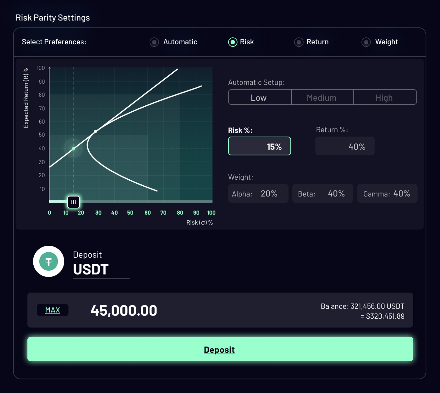
Figure 15: Deposit Screen for Parity

Alpha, Beta and Gamma are our three main funds with different levels of risk and expected returns. Alpha will be more risky than Beta, which will be more risky than Gamma. Investors will be able to combine the three funds depending on their risk appetites using a suitable Graphical User Interface (GUI - Figure 15; Martinez 2011; End-note 22). Mixing Alpha, Beta and Gamma will give the Risk Parity portfolio. Risk Parity will generate returns for investors that factor the risk of the individual assets, with each asset contributing equally to the overall risk of the portfolio. The end result will be the first investment vehicle that will tailor the preferences of each investor - providing diversified and risk adjusted returns - entirely on a highly secure blockchain environment.

A subtle aspect of our portfolio construction and the weight calculation methodology described in Kashyap (2022) is that parity is already accomplished in each of our individual funds Alpha, Beta and Gamma. These investment products - Alpha, Beta, Gamma and Parity - will provide risk managed access to several crypto assets and strategies. We have adapted many of the well known safety mechanisms and investor protection schemes that have evolved for several decades in traditional finance, and combined them with many innovations that are unique to crypto markets (Kashyap 2023).

Having mentioned that each of our sub funds already achieves risk parity, we need to draw a distinction between mathematical parity and conceptual parity. The assets weights are calculated based on precise rules and mathematical operations and this brings parity to each of our sub funds at the asset level. While this is still a huge innovation to bring to the blockchain environment, we wish to proceed further and bring parity also on a conceptual level.

To elaborate further, we create portfolios that perform satisfactorily where mathematics can fall short of completely combating market uncertainty. Broad categories of assets have slightly different risk and return attributes. By grouping assets with similar responses to different market regimes, we can ensure that the various groups counterbalance one another under diverse market conditions. Hence, in addition to mathematical parity, within each sub fund, each sub fund has an overall risk return feature which is preferable to the other sub funds under a particular market criterion.

Another motivation for creating these groups is because even if assets at the individual level deviate from their risk and expected return properties, such a misalignment is less likely at the group level. A few assets in a bunch might display atypical behavior, but the majority of them will be closer to their representative qualities. The result is that the overall group can be expected to behave in a certain way and offset other groups, which are constructed based on the same principle of clubbing together similar assets, that have different attributes. We term this fluctuating pseudo-equilibrium between groups of assets conceptual parity.

The implication of constructing the sub-funds (Alpha, Beta and Gamma) in this way ensures that when the overall market under performs, which means Alpha and Beta will not deliver very high returns, Gamma will still continue to provide acceptable returns because of its negative correlation to Alpha and Beta. The manufacturing, and linking, of Alpha, Beta and Gamma will then produce the most efficient set of portfolios in terms of risk and return characteristics. We term this collection of portfolios, the parity line.

Risk Parity is a unique advance in cross-chain DeFi asset management. The Parity index class is where all our other index classes (Alpha, Beta and Gamma) come together. In addition to the balanced portfolios created by the other indexes, the Risk Parity strategy provides cover against universal changes such as higher than expected inflation, which could otherwise negatively affect most portfolios, both crypto and traditional.

Risk Parity is an investment movement first pioneered in the All Weather fund by Ray Dalio at Bridgewater Associates in 1996 (Prince 2011; Fabozzi, et al. , 2021). It aims to return results better than holding cash no matter the circumstances. Many investment managers try to diversify assets but ignore the wider environmental risks, such as inflation or low economic growth that can have a major impact on the entire economy. Some examples of such events are: recessions, the 2008 financial crisis or indeed a global pandemic (Reinhart & Rogoff 2008; Acharya & Richardson 2009; Ciotti et al., 2020). It is generally true to a large extent that the wider economic outlook is ‘priced in’ to assets. The risk materializes when expectations aren’t met, in either direction. Additional pointers regarding this topic are mentioned in Section (6).

Risk Parity was designed to enable a portfolio to perform whatever the environment. Until now, this extraordinarily successful mechanism from traditional finance could not be applied to crypto because the tools didn’t exist. This work - and its sister papers - is the first to engineer the necessary infrastructure, along with the required foundational principles, to bring such a risk managed portfolio to DeFi cross-chain assets.

5 On Par With Parity: The Mathematics of Mixing Alpha, Beta and Gamma

We modify well known techniques in portfolio management theory related to obtaining portfolios on the efficient frontier. We note that our problem boils down to being able to combine three funds: Alpha, Beta and Gamma using a robust and simple methodology to obtain an ideal fund that balances risk and return. We refer to this combined fund as the Parity Portfolio. The properties of the individual funds are discussed in separate articles (Kashyap 2022). The essence of the properties of the three portfolios are that each fund caters to a varying risk appetite. In addition, the Gamma fund is constructed such that it shows negative correlation to Alpha to a certain extent and also to Beta at times. Hence combining the three funds provides an all weather portfolio, or a portfolio that outperforms the market during both upturns and downturns.

The efficient frontier is an extremely elegant approach to finding excellent combinations of risk and return. To simplify the corresponding ideas for a blockchain environment and also to make sure the solutions are more robust, we formulate the ideas as linear approximations. The linear approximation becomes valid as we construct Gamma portfolios that show negative correlation to Alpha and Beta. These approximations can easily be modified in later versions of the application, but the main idea is that this approach allows the weights corresponding to specific combinations of risk and return to be calculated on-chain.

The simplifications we adopt can also enable moving these calculations onto an on-chain framework quite seamlessly using smart contracts (Zou, et al., 2019; Zheng, et al., 2020; End-note 23). As better blockchain networks develop, we will need to see if the above techniques we have created need modification. It might be possible to use thousands of transactions for calculations on a blockchain computing platform. To emphasize, committing thousands of transactions to the blockchain record, or into a block, is already possible (Pierro & Tonelli 2022). The basics of computing make it clear that the more data we wish to store and the more computations we need to perform, the associated costs will increase (Dromey 1982).

The other reasons for adopting linear approximations are because the efficient frontier is based on estimates of risk and return, which can be highly erroneous. So instead of estimating several parameters to get a curve that acts as the efficient frontier, we fit a line - through regression or other methodologies at a later stage - across the set of diversified fund portfolios we have created (Alpha, Beta, Gamma) over time. That is the as the points Alpha, Beta and Gamma move over time, they give us a measure of how the Parity Line is changing with time.

5.1 The Parity Line: The Final Frontier Of Asset Management

In terms of the three funds, Alpha is the most risky and hence has the highest expected return. Beta comes second in terms of risk and Gamma is the least risky of the three. Hence, Alpha also provides the highest expected returns and so on. If we visualize these three funds as points on a graph with risk (standard deviation of returns) on the X-axis and expected return on the Y-axis (Figures 2; 4). Alpha would be the right most point. Beta would be in the middle and Gamma would be the leftmost point.

As expectations change with time and as the market changes, risk and expected return of the funds will change over time. Hence we need to visualize the three funds as clouds of points in the right, middle and left of the graph (Figure 2). We can fit a regression line through these points and we will let investors chose what level of risk and return they want based on the slope and intercept of this line. This line is a really good estimate of the best portfolios that investors can chose and we term this the Parity Line. Since this is a modification of the concept of the efficient frontier, this Parity Line becomes the final frontier of investments. We denote this line as:

$$E\left(R\right)=\left(\Theta\right)\left(\sigma\right)+R_{F}$$ (1)

Here, $E\left(R\right)$ is the expected return. $\sigma$ is the risk. $\Theta$ and $R_{F}$ are the slope and the intercept of the line respectively. Notice that the intercept, $R_{F}$, is also the risk free rate. We calculate the slope and intercept separately using regression or other methods and store them in the smart contract.

Any investor can chose a level of risk and his expected return will be fixed based on the efficient Parity Line. Likewise if someone chooses a certain level of expected return, the risk they need to bear to achieve that will be given by the efficient Parity Line. In addition, investors can also choose the proportion of their wealth they can allocate to Alpha, Beta and Gamma directly. Based on this allocation of wealth, we determine the expected return and risk the investors wealth would bear on the efficient Parity Line. $E\left(R_{\alpha}\right)$ is the expected return and $\sigma_{\alpha}$ is the risk of Alpha. $E\left(R_{\beta}\right)$ is the expected return and $\sigma_{\beta}$ is the risk of Beta. $E\left(R_{\gamma}\right)$ is the expected return and $\sigma_{\gamma}$ is the risk of Gamma. The weights invested into Alpha, Beta and Gamma for investor $i$ are represented by $w_{\alpha}$ , $w_{\alpha}$ and $w_{\alpha}$ respectively. The expected return and risk are estimated using Equations (204; 206) in Section (13).

For each investor we mint an NFT (Kugler 2021; Wang et al., 2021; Bao & Roubaud 2022; End-note 24) that stores at a minimum the following information: the amount being deposited, their risk and expected return preferences and the weight allocation of their wealth into Alpha, Beta and Gamma portfolios. We consider the three scenarios below:

1. Investor Chooses Risk Tolerance: The investor can choose his / her level of risk tolerance, $\sigma_{i}$, on a sliding scale. From this, we will calculate the other values to store in the NFT.

   $$E\left(R_{i}\right)=\left(\Theta\right)\left(\sigma_{i}\right)+R_{F}$$ (2)

   The weights to be invested into Alpha, Beta and Gamma are given by calculating the distance to the Alpha, Beta and Gamma points from the investors risk and expected return point, $P\equiv\left[\sigma_{i},E\left(R_{i}\right)\right]$, on the efficient Parity Line. We denote the distance between two points $A\equiv\left[\sigma_{A},E\left(R_{A}\right)\right]$ and $B\equiv\left[\sigma_{B},E\left(R_{B}\right)\right]$ as $d_{A,B}$ (Rudin 1953; End-note 25).

   $$w_{\alpha}=\frac{\left(\frac{1}{d_{\alpha,P}}\right)}{\left[\left(\frac{1}{d_{\alpha,P}}\right)+\left(\frac{1}{d_{\beta,P}}\right)+\left(\frac{1}{d_{\gamma,P}}\right)\right]}$$ (3)

   $$w_{\beta}=\frac{\left(\frac{1}{d_{\beta,P}}\right)}{\left[\left(\frac{1}{d_{\alpha,P}}\right)+\left(\frac{1}{d_{\beta,P}}\right)+\left(\frac{1}{d_{\gamma,P}}\right)\right]}$$ (4)

   $$w_{\gamma}=\frac{\left(\frac{1}{d_{\gamma,P}}\right)}{\left[\left(\frac{1}{d_{\alpha,P}}\right)+\left(\frac{1}{d_{\beta,P}}\right)+\left(\frac{1}{d_{\gamma,P}}\right)\right]}$$ (5)

   $$d_{A,B}=\sqrt{\left(\sigma_{A}-\sigma_{B}\right)^{2}+\left(E\left(R_{A}\right)-E\left(R_{B}\right)\right)^{2}}$$ (6)

   $$d_{\alpha,P}=\sqrt{\left(\sigma_{\alpha}-\sigma_{i}\right)^{2}+\left(E\left(R_{\alpha}\right)-E\left(R_{i}\right)\right)^{2}}$$ (7)

   Note that the weights satisfy the equation,

   $$w_{\alpha}+w_{\beta}+w_{\gamma}=1$$ (8)

   If any of the distances are zero, the corresponding weight becomes 1. That is, $w_{\alpha}=1$ if $d_{\alpha,P}=0$ and so on.

2. Investor Chooses Expected Return Level: The investor can choose his / her level of expected return, $E\left(R_{i}\right)$, on a sliding scale. From this, we will calculate the other values to store in the NFT.

   $$\sigma_{i}=\frac{E\left(R_{i}\right)-R_{F}}{\left(\Theta\right)}$$ (9)

   The weights are calculated similar to Point (1) above.

3. Investor Chooses Alpha, Beta and Gamma Weights: The investor can choose his allocations to each of the three funds directly. He will choose two and the third is given by the identify, $w_{\alpha}+w_{\beta}+w_{\gamma}=1$. From this, we will calculate the other values to store in the NFT.

   $$E\left(R_{i}\right)=\left[w_{\alpha}E\left(R_{\alpha}\right)\right]+\left[w_{\beta}E\left(R_{\beta}\right)\right]+\left[w_{\gamma}E\left(R_{\gamma}\right)\right]$$ (10)

   $$\sigma_{i}=\left(w_{\alpha}\sigma_{\alpha}\right)^{2}+\left(w_{\beta}\sigma_{\beta}\right)^{2}+\left(w_{\gamma}\sigma_{\gamma}\right)^{2}+2w_{\alpha}\sigma_{\alpha}w_{\beta}\sigma_{\beta}\rho_{\alpha,\beta}+2w_{\beta}\sigma_{\beta}w_{\gamma}\sigma_{\gamma}\rho_{\beta,\gamma}+2w_{\alpha}\sigma_{\alpha}w_{\gamma}\sigma_{\gamma}\rho_{\alpha,\gamma}$$ (11)

   Here, $\rho_{\alpha,\beta}$ represents the correlation between Alpha and Beta. If the correlation values are not readily available, we can use our Parity Line to get the value of risk to store in the NFT using Point (2) and the expected return from Equation (10). This approximation is valid to a reasonable extent since the Parity Line is the best combination of risk and expected returns possible and the user’s wealth allocation will result in a point on this line. Figure (3) shows an example of calculating the combined portfolio return and risk when the weights of Alpha, Beta and Gamma are calculated using the volatilities of the funds themselves.

5.2 Distancing the Distance Function

The approximation in Point (3) in Section (5.1) also has a related problem. If we use the Euclidean distance functions specified in Point (1) and Section (5.1) we note that there are many possible solutions to go from weights to risk and expected return as discussed in Point (3). Specifically, let us say we chose a particular risk and return combination and then get the Alpha, Beta and Gamma weights corresponding to this choice of risk and return. Now, if we use these weights and try to calculate the risk and the return we may not get the same risk and return combination we originally started with. This is because the distance function has many points on the risk-return plane that satisfy the corresponding constraints on the parity line.

An alternative approach is to combine Alpha and Beta portfolios with weights $w_{c\alpha}$ and $w_{c\beta}$ to form a combined portfolio, or market portfolio, that lies on the parity line. We denote the expected return and risk of this combined portfolio as $E\left(R_{c}\right)$ and $\sigma_{c}$ respectively.

$$E\left(R_{c}\right)=\left[w_{c\alpha}E\left(R_{\alpha}\right)\right]+\left[w_{c\beta}E\left(R_{\beta}\right)\right]$$ (12)

Using the slope and intercept of the parity line we get,

$$\sigma_{c}=\frac{E\left(R_{c}\right)-R_{F}}{\left(\Theta\right)}$$ (13)

We can then select the weights for Alpha, Beta and Gamma based on the risk and expected return preferences of any investor, $\sigma_{i}$ and $E\left(R_{i}\right)$. First we get the weights to be invested in Gamma and the combined portfolio ($w_{c}$) as follows,

$$w_{c}=\frac{\left[E\left(R_{i}\right)-E\left(R_{\gamma}\right)\right]}{\left[E\left(R_{c}\right)-E\left(R_{\gamma}\right)\right]}$$ (14)

$$w_{\gamma}=\frac{\left[E\left(R_{i}\right)-E\left(R_{c}\right)\right]}{\left[E\left(R_{\gamma}\right)-E\left(R_{c}\right)\right]}$$ (15)

Note that the weights for Gamma and the combined portfolio can be negative or greater than one if the user’s risk and return preference lies above the risk and return of the combined portfolio. This condition can be expressed as,

$$\sigma_{i}>\sigma_{c}\text{ or }E\left(R_{i}\right)>E\left(R_{c}\right)$$ (16)

We can trim the weights for Gamma and the combined portfolio when they are negative or greater than one by using suitable bounds. This gives the weight to be invested in Alpha and Beta as,

$$w_{\alpha}=\left(w_{c}\right)\left(w_{c\alpha}\right)$$ (17)

$$w_{\beta}=\left(w_{c}\right)\left(w_{c\beta}\right)$$ (18)

Proposition 1.

If the weights for Alpha, Beta and Gamma are chosen as below

$$w_{\alpha}=\left(w_{c}\right)\left(w_{c\alpha}\right)$$ (19)

$$w_{\beta}=\left(w_{c}\right)\left(w_{c\beta}\right)$$ (20)

$$w_{\gamma}=\frac{\left[E\left(R_{i}\right)-E\left(R_{c}\right)\right]}{\left[E\left(R_{\gamma}\right)-E\left(R_{c}\right)\right]}$$ (21)

We then get the expected return chosen by the investor. That is,

$$\left[w_{\alpha}E\left(R_{\alpha}\right)\right]+\left[w_{\beta}E\left(R_{\beta}\right)\right]+\left[w_{\gamma}E\left(R_{\gamma}\right)\right]=E\left(R_{i}\right)$$ (22)

Proof.

Appendix (12.1). ∎

There is still the possibility that multiple combinations of weights can give the same risk and return on the parity line. But the above approach ensures that the weights we obtain for any risk and return chosen will give back the same risk and return.

Figure (4) has numerical examples illustrating this methodology of combining Alpha, Beta and Gamma. Figures (5; 6; 7; 8) show several scenarios where the risk and return of the parity portfolio are calculated depending on the risk and return of Alpha, Beta and Gamma with investors choosing their desired level of risk, return or the weights of the sub-funds. In the scenarios either the investor choice of portfolio risk or the return are increased in steps of one percent or the weights are incremented suitably to get portfolio risk or return increments of one percent.

5.3 Robust and Simple Estimation of The Parity Line

Note that the Parity Line will change over time. Hence, as time passes we will periodically change the slope and intercept of the Parity Line that is stored in the smart contract (Figure 2).

One approach to decide when to seed the smart contract with new values of the slope and intercept for the Parity Line are to use the volatility of Alpha, Beta and Gamma and when a new point lies outside a circle based on the corresponding volatility, it is a good indicator to change the Parity Line.

A very simple approach to obtain the Parity Line is to run a regression across different values of return and risk of Alpha, Beta and Gamma over time. The issue with this approach is that the newer values of Alpha, Beta and Gamma do not get any additional weight or priority. To resolve this, we can use advanced regression techniques or take a weighted average of the values giving higher weight to recent values and run the regression with these weighted average values.

Other than regression methods, the Parity Line can be chosen as the line passing through Alpha and Beta. This is for simplicity and also because a simple regression line will not give more preference to recent values of Alpha, Beta and Gamma. We are using Alpha and Beta since by design they are higher than Gamma on the return or Y-axis. But the Parity Line is the line passing through the two points that have the highest and second highest return with positive slope. We emphasize the positive slope since due to market movements and related anomalies, Beta could be higher than Alpha resulting in negative slope. In this case, the Parity Line will be the one that passes through Alpha and Gamma or Beta and Gamma, if Beta is only slightly higher than Alpha on the return axis.

The main point to note is that the choice of the parameters of the Parity Line will be done off-chain and the calculated values will then be stored in the smart contract and updated when deemed necessary.

Though, we need to know what choice the investor made and using that choice we need to calculate the other values and update the NFT accordingly. When the weights chosen by the investor and the weights implied by the Parity Line are different, a simple rebalancing can be performed (Section 5.4).

5.4 Parity Rebalancing

Once an investor makes an investment into Parity and the weights for Alpha, Beta and Gamma investment are finalized, the corresponding amounts are invested into Alpha, Beta and Gamma. Hence, based on the total investment and the individual weights, token quantities specific to the investment amounts into each of Alpha, Beta and Gamma will be allocated to the investor. This allocation can be stored in the NFT or it can also be stored in the smart contract. This will depend on the pros and cons of adding / storing more metadata into the NFT and is a technical design consideration.

The intrinsic value of the NFT, $PARITYINTRINSICVALUE_{it}$, held by investor $i$ at any time $t$ is the sum of the Alpha, Beta and Gamma quantities ($ALPHAQTY_{it}$, $BETAQTY_{it},$$GAMMAQTY_{it}$) allocated to the investor multiplied by the corresponding asset prices ($ALPHAPRICE_{t},$$BETAPRICE_{t}$,$GAMMAPRICE_{t}$).

$$PARITYINTRINSICVALUE_{it} =\left(ALPHAQTY_{it}\right)\left(ALPHAPRICE_{t}\right)$$ (23)

$$+\left(BETAQTY_{it}\right)\left(BETAPRICE_{t}\right)$$ (24)

$$+\left(GAMMAQTY_{it}\right)\left(GAMMAPRICE_{t}\right)$$ (25)

There are three primary causes for changing the tokens allocated to any investors:

1. When the prices of the assets change over time, the contribution of Alpha, Beta and Gamma to the intrinsic value of Parity will change. Hence, there will be a deviation from the weights chosen by the investor. A rebalancing mechanism is required that will bring the weights back to the chosen weights. Note that this adjustment is similar to the other two cases.

2. When the weights will change due to changes in the user preferences or

3. Due to changes in the Parity Line.

We consider how to move assets across Alpha, Beta and Gamma based on the changes due to the above three contributing causes and also to meet investor deposit and withdrawal requests in Section (5.4.1). The goal of these fund movements are to keep investor aligned with their risk and return objectives.

5.4.1 Parity Sequence of Steps

To outline the main sequence of steps, and the corresponding calculations, for the Parity investment process we proceed with the steps given in Algorithm (1) as follows:

Algorithm 1.

The following algorithm captures the sequence of steps that need to be carried out at periodic intervals to ensure that the investments in Alpha, Beta and Gamma can capture the risk and return preferences and also deposit and withdrawal requests from all investors entirely on blockchain. The algorithm also takes of the changes in the allocations - across Alpha, Beta and Gamma- for the investors based on changes in the market environment and the risk profiles of the individual funds.

1. Calculate new Net Asset Value (NAV: Penman 1970; End-note 27) or Fund Prices for Alpha, Beta and Gamma based on Step (1) and Step (2) in Kashyap (2023).

2. In addition to the variables in Equation (23), we need to also consider pending deposits and withdraw requests made by any investor to give the complete intrinsic value of the Parity investment held by that investor.

   1. We next calculate the value of the tokens plus any pending deposits held by investor $i$ at time $t$, $PARITYDPLUST_{it}$.We then calculate the value of the withdraw request made by investor $i$ at time $t$, $PARITYWDRW_{it}$. The deposit amount which has still not been converted to tokens for investor $i$ at time $t$ is $DEPOSIT_{it}$. The deposit amount at this phase of the project will be in a stable token or denominated in USD (Ante, Fiedler & Strehle 2021; Grobys et al., 2021; Hoang & Baur 2021; Lyons & Viswanath-Natraj 2023; End-note 26). The withdraw amount will be specified as a percentage of the intrinsic value held by the investor, $WITHDRAW_{it}$. Note that, $0\leq WITHDRAW_{it}\leq 1$.

      $$PARITYDPLUST_{it} =DEPOSIT_{it}+\left(ALPHAQTY_{it}\right)\left(ALPHAPRICE_{t}\right)$$ (26)

      $$+\left(BETAQTY_{it}\right)\left(BETAPRICE_{t}\right)$$ (27)

      $$+\left(GAMMAQTY_{it}\right)\left(GAMMAPRICE_{t}\right)$$ (28)

      $$PARITYWDRW_{it} =WITHDRAW_{it}\left[DEPOSIT_{it}\right.$$ (29)

      $$+\left(ALPHAQTY_{it}\right)\left(ALPHAPRICE_{t}\right)$$ (30)

      $$+\left(BETAQTY_{it}\right)\left(BETAPRICE_{t}\right)$$ (31)

      $$\left.+\left(GAMMAQTY_{it}\right)\left(GAMMAPRICE_{t}\right)\right]$$ (32)

      $$PARITYWDRW_{it} =\left(WITHDRAW_{it}\right)\left(PARITYDPLUST_{it}\right)$$ (33)

      The value available for future withdraw requests for investor $i$ at time $t$ is given by, $PARITYAVLWDRW_{it}$.

      $$PARITYAVLWDRW_{it} =\left(PARITYDPLUST_{it}\right)\left(1-WITHDRAW_{it}\right)$$ (34)

   2. Additional deposits and withdraw requests, made before the sequence of steps are run, results in the cumulation of the deposit and withdraw amounts in the pending state. That is, the deposit is a summation of the deposits from time $T$ to the present time $t$. With a slight abuse of notation which is helpful while writing this in computer code wherein the final calculated values can be saved back into the original variables, we write this as,

      $$DEPOSIT_{it}=\sum_{l=T}^{l=t}DEPOSIT_{il}\quad\begin{cases}T\leq l\leq t\end{cases}$$ (35)

      Here $T$ is the time when the previous rebalance is completed. All deposits made by the investor since $T$ are added to the deposit balance at $T$. Note that, the deposit balance at $T$ can be greater than zero if a large deposit was made and it was not fully invested into the sub-funds Alpha, Beta and Gamma when the sequence of steps are completed at $T$. That is $DEPOSIT_{iT}\geq 0$.

   3. Likewise, the withdraw amount at time $t$, can be calculated by initially setting the amount available to withdraw to the sum of the pending deposit and token values. This is done when the first withdraw request is made. We use this available amount to calculate the withdraw amounts from subsequent requests and then cumulate them until time $t$

      $$PARITYAVLWDRW_{it} =PARITYDPLUST_{it}$$ (36)

      $$PARITYWDRW_{it}=PARITYAVLWDRW_{it} \left(WITHDRAW_{it}\right)$$ (37)

      $$PARITYAVLWDRW_{it} =PARITYAVLWDRW_{it}\left(1-WITHDRAW_{it}\right)$$ (38)

      $$PARITYWDRW_{it}= PARITYWDRW_{iT}$$ (39)

      $$+ \sum_{l=T}^{l=t}PARITYAVLWDRW_{it}\left(WITHDRAW_{it}\right)$$ (40)

      $$\quad\begin{cases}T\leq l\leq t\end{cases}$$ (41)

      Here $T$ is the time when the previous rebalance is completed. All deposits made by the investor since $T$ are added to the deposit balance at $T$. Note that, the withdraw balance at $T$ can be greater than zero if a large withdraw request was made and it was not fully redeemed from the sub-funds Alpha, Beta and Gamma when the sequence of steps are completed at $T$. That is, $PARITYWDRW_{iT}\geq 0$.

   4. The deposit and withdraw variables are incremented whenever the user makes an action. This ensures that the latest deposit or withdraw variable state is obtained and the gas fees for the operations to keep these variables updated are paid by the investor as a part of of the deposit or withdraw transaction.

3. The deposit amount and the withdraw amount will be netted for each user. Please note that the netting can be done along with each deposit or withdraw user action. It is tempting to do the netting only after the Parity sequence of steps have commenced and the Alpha, Beta and Gamma prices have been updated. But since we are only using the cash deposit made by the user to fulfill his / her withdraw request, the netting can happen whenever the user makes a deposit or withdraw action.

   1. We will have a net deposit or withdraw depending on which cashflow is bigger. That is we check the condition, $DEPOSIT_{it}\geq PARITYWDRW_{it}$ and calculate the net inflow $PARITYINFLOW_{it}$ or outflow $PARITYOUTFLOW_{it}$ as follows,

      $$PARITYINFLOW_{it} =\begin{cases}\begin{array}[]{cc}DEPOSIT_{it}-PARITYWDRW_{it}&DEPOSIT_{it}\geq PARITYWDRW_{it}\\ 0&DEPOSIT_{it}<PARITYWDRW_{it}\end{array}\end{cases}$$ (42)

      $$PARITYOUTFLOW_{it} =\begin{cases}\begin{array}[]{cc}0&DEPOSIT_{it}\geq PARITYWDRW_{it}\\ PARITYWDRW_{it}-DEPOSIT_{it}&DEPOSIT_{it}<PARITYWDRW_{it}\end{array}\end{cases}$$ (43)

      Or this can be written alternatively as,

      $$PARITYINFLOW_{it} =\max\left(DEPOSIT_{it}-PARITYWDRW_{it},0\right)$$ (44)

      $$PARITYOUTFLOW_{it} =\max\left(PARITYWDRW_{it}-DEPOSIT_{it},0\right)$$ (45)

      Note that only one variable, $PARITYINFLOW_{it}$ or $PARITYOUTFLOW_{it}$ can be positive and the other variable has to be zero. While writing this in computer code, the inflow and outflow values can be saved back into the original variables. See sub-point (3b) for additional clarifications.

   2. The Equations (44; 45) in sub-point (3a) need to be modified, to include the cash received from a previous rebalancing for the investor along with the deposits, to get the full inflow amount. This is discussed in sub-point (7g) and given in Equations (171; 172). The aggregate level (or across investors) cash allocations are discussed in sub-point (7h) and given in Equations (173; 174). Also sub-points (5e; 5f) for aggregate (across investors) level calculations.

   3. Using these variables gives the intrinsic value of Parity that includes deposits and withdraw requests. The intrinsic value of the NFT, $PARITYINTRINSICVALUE_{it}$, held by investor $i$ at any time $t$ is the sum of the Alpha, Beta and Gamma quantities ($ALPHAQTY_{it}$, $BETAQTY_{it},$ $GAMMAQTY_{it}$) allocated to the investor multiplied by the corresponding asset prices ($ALPHAPRICE_{t},$ $BETAPRICE_{t}$, $GAMMAPRICE_{t}$) including the inflow and outflow of funds, $PARITYINFLOW_{it}$ or $PARITYOUTFLOW_{it}$.

      $$PARITYINTRINSICVALUE_{it} =PARITYINFLOW_{it}$$ (46)

      $$+\left(ALPHAQTY_{it}\right)\left(ALPHAPRICE_{t}\right)$$ (47)

      $$+\left(BETAQTY_{it}\right)\left(BETAPRICE_{t}\right)$$ (48)

      $$+\left(GAMMAQTY_{it}\right)\left(GAMMAPRICE_{t}\right)$$ (49)

      $$-PARITYOUTFLOW_{it}$$ (50)

4. The weights of Alpha, Beta and Gamma, for investor $i$ at time $t$ are ($ALPHAWGT_{it}$, $BETAWGT_{it}$, $GAMMAWGT_{it}$). Based on these weights we can calculate the quantities that are supposed to be invested into Alpha, Beta and Gamma, ($INVALPHAQT$, $INVBETAQTY_{it}$, $INVGAMMAQTY_{it}$), for investor $i$ at time $t$.

   $$INVALPHAQTY_{it} =\frac{PARITYINTRINSICVALUE_{it}\left(ALPHAWGT_{it}\right)}{\left(ALPHAPRICE_{t}\right)}-ALPHAQTY_{it}$$ (51)

   $$INVBETAQTY_{it} =\frac{PARITYINTRINSICVALUE_{it}\left(BETAWGT_{it}\right)}{\left(BETAPRICE_{t}\right)}-BETAQTY_{it}$$ (52)

   $$INVGAMMAQTY_{it} =\frac{PARITYINTRINSICVALUE_{it}\left(GAMMAWGT_{it}\right)}{\left(GAMMAPRICE_{t}\right)}-GAMMAQTY_{it}$$ (53)

   1. Clearly the above can be written in dollar notational values ($INVALPHAAMNT_{it}$, $INVBETAAMNT_{it}$, $INVGAMMAAMNT_{it}$) to be invested into Alpha, Beta and Gamma for investor $i$ at time $t$ as,

      $$INVALPHAAMNT_{it} =PARITYINTRINSICVALUE_{it}\left(ALPHAWGT_{it}\right)$$ (54)

      $$-ALPHAQTY_{it}\left(ALPHAPRICE_{t}\right)$$ (55)

      $$INVBETAAMNT_{it} =PARITYINTRINSICVALUE_{it}\left(BETAWGT_{it}\right)$$ (56)

      $$-BETAQTY_{it}\left(BETAPRICE_{t}\right)$$ (57)

      $$INVGAMMAAMNT_{it} =PARITYINTRINSICVALUE_{it}\left(GAMMAWGT_{it}\right)$$ (58)

      $$-GAMMAQTY_{it}\left(GAMMAPRICE_{t}\right)$$ (59)

   2. Since the deposit amounts are in USD and the withdraw quantities are denominated in tokens we can separate these out, for each investor $i$ at time $t$, in USD investment amounts and token withdraw quantities. This also ensures we are only storing positive values depending on whether we are making a net deposit or withdraw as shown below,

      $$INVALPHAAMNT_{it} =\max\left[PARITYINTRINSICVALUE_{it}\left(ALPHAWGT_{it}\right)\right.$$ (60)

      $$-\left.ALPHAQTY_{it}\left(ALPHAPRICE_{t}\right),0\right]$$ (61)

      $$WDRWALPHAQTY_{it} =\max\left[ALPHAQTY_{it}-\frac{PARITYINTRINSICVALUE_{it}\left(ALPHAWGT_{it}\right)}{\left(ALPHAPRICE_{t}\right)},0\right]$$ (62)

      ($WDRWALPHAQTY_{it}$, $WDRWBETAQTY_{it}$, $WDRWGAMMAQTY_{it}$) are the quantities to be withdrawn from Alpha, Beta and Gamma for investor $i$ at time $t$. Notice that only one of $INVALPHAAMNT_{it}$ or $WDRWALPHAQTY_{it}$ can be non-zero (and positive). The same applies to the other pairs of variables for Beta and Gamma.

      $$INVBETAAMNT_{it} =\max\left[PARITYINTRINSICVALUE_{it}\left(BETAWGT_{it}\right)\right.$$ (63)

      $$-\left.BETAQTY_{it}\left(BETAPRICE_{t}\right),0\right]$$ (64)

      $$WDRWBETAQTY_{it} =\max\left[BETAQTY_{it}-\frac{PARITYINTRINSICVALUE_{it}\left(BETAWGT_{it}\right)}{\left(BETAPRICE_{t}\right)},0\right]$$ (65)

      $$INVGAMMAAMNT_{it} =\max\left[PARITYINTRINSICVALUE_{it}\left(GAMMAWGT_{it}\right)\right.$$ (66)

      $$-\left.GAMMAQTY_{it}\left(GAMMAPRICE_{t}\right),0\right]$$ (67)

      $$WDRWGAMMAQTY_{it} =\max\left[GAMMAQTY_{it}-\frac{PARITYINTRINSICVALUE_{it}\left(GAMMAWGT_{it}\right)}{\left(GAMMAPRICE_{t}\right)},0\right]$$ (68)

   3. Also the following simple identity must be satisfied when the deposit and withdraw values are combined with the amounts being moved across funds (rebalancing) so that the investor stays aligned with their Alpha, Beta and Gamma weights.

      $$PARITYINFLOW_{it}+\left(ALPHAPRICE_{t}\right)WDRWALPHAQTY_{it}$$ (69)

      $$+\left(BETAPRICE_{t}\right)WDRWBETAQTY_{it}+\left(GAMMAPRICE_{t}\right)WDRWGAMMAQTY_{it}$$ (70)

      $$=$$ (71)

      $$PARITYOUTFLOW_{it}+INVALPHAAMNT_{it}$$ (72)

      $$+INVBETAAMNT_{it}+INVGAMMAAMNT_{it}$$ (73)

5. We then aggregate the total deposit amounts and withdraw quantities across all investors. There are two possible groups to aggregate.

   1. First, across all users. This will be done after a parity line change or a global rebalance for everyone.

   2. Second, the other group of users will be those that have a non zero deposit or withdraw. This second group of users is used on a periodic basis for getting the total amounts to deposit or withdraw from Alpha, Beta and Gamma and also to allocate what is received from the sub-funds.

   3. Clearly, any group of users can be chosen for the aggregation depending on the situation dictated by gas fees or other considerations. This applies to sub-point (5a) as well if there are a large number of users and we need to rebalance them in batches.

   4. Another way to prioritize users to rebalance would be to check their total amount for rebalancing and order based on the users with the highest amounts for rebalancing. The amount for rebalancing will be given by the sum of the difference between the actual allocation and expected allocation across all three funds: Alpha, Beta and Gamma (ABG). We denote the total amount to rebalance for investor $i$ at time $t$ , $TOTALRBLNC_{it}$,by the following,

      $$TOTALRBLNC_{it} =PARITYINFLOW_{it}$$ (74)

      $$+\left(ALPHAPRICE_{t}\right)WDRWALPHAQTY_{it}$$ (75)

      $$+\left(BETAPRICE_{t}\right)WDRWBETAQTY_{it}$$ (76)

      $$+\left(GAMMAPRICE_{t}\right)WDRWGAMMAQTY_{it}$$ (77)

      $$+PARITYOUTFLOW_{it}+INVALPHAAMNT_{it}$$ (78)

      $$+INVBETAAMNT_{it}+INVGAMMAAMNT_{it}$$ (79)

      Note here that we also include deposits and withdraws pending since that is a complete treatment of the total fund flows required for investor $i$ at time $t$ .

   5. If we let $IC_{t}$ denote the total number or count of investors being considered for aggregation at time $t$ the below variables, prefixed with $PA...$ for Parity Aggregate, represent the totals across all investors,

      $$PAINVALPHAAMNT_{t}=\sum_{i=1}^{i=IC_{t}}INVALPHAAMNT_{it}$$ (80)

      $$PAWDRWALPHAQTY_{t} =\sum_{i=1}^{i=IC_{t}}WDRWALPHAQTY_{t}$$ (81)

      $$PAINVBETAAMNT_{t} =\sum_{i=1}^{i=IC_{t}}INVBETAAMNT_{it}$$ (82)

      $$PAWDRWBETAQTY_{t} =\sum_{i=1}^{i=IC_{t}}WDRWBETAQTY_{it}$$ (83)

      $$PAINVGAMMAAMNT_{t} =\sum_{i=1}^{i=IC_{t}}INVGAMMAAMNT_{it}$$ (84)

      $$PAWDRWGAMMAQTY_{t} =\sum_{i=1}^{i=IC_{t}}WDRWGAMMAQTY_{it}$$ (85)

      The net fund flows across all investors in terms of deposits and withdraw requests is given by,

      $$PARITYINFLOW_{t}=DEPOSIT_{t}=\sum_{i=1}^{i=IC_{t}}DEPOSIT_{it}=\sum_{i=1}^{i=IC_{t}}PARITYINFLOW_{it}$$ (86)

      $$PARITYOUTFLOW_{t}=PARITYWDRW_{t}=\sum_{i=1}^{i=IC_{t}}PARITYWDRW_{it}=\sum_{i=1}^{i=IC_{t}}PARITYOUTFLOW_{it}$$ (87)

      Note that we need to include any cash received from a previous rebalancing for all the investors along with the deposits to get the full inflow amount. These aggregate (across investors) level cash inclusions are discussed in sub-point (7h) and given in Equations (173; 174). The investor level cash allocations are discussed in sub-point (7g) and given in Equations (171; 172).See sub-point (5f) for aggregate level calculations such that only the investment or withdraw side is positive. See sub-points (3a; 3b) for additional clarifications related to the investor level deposit and cash inclusions.

   6. Notice that we net again at the fund level (Parity Aggregate) such that only one of $PAINVALPHAAMNT_{t}$ or $PAWDRWALPHAQTY_{t}$ can be non-zero (and positive). See sub-point (5e) for additional context. The same applies to the other pairs of variables for Beta and Gamma. We highlight here that the modified values that include pending amounts need to be considered as shown in Point (5h). The calculations in this step are helpful to arrive at the Parity fund flow identity in Point (5g) and the allocations in Point (7).

      $$PAINVALPHAAMNT_{t} =\max\left[\sum_{i=1}^{i=IC_{t}}INVALPHAAMNT_{it}\right.$$ (88)

      $$-\left.\left(ALPHAPRICE_{t}\right)\sum_{i=1}^{i=IC_{t}}WDRWALPHAQTY_{it},0\vphantom{\sum_{i=1}^{i=IC_{t}}}\right]$$ (89)

      $$PAWDRWALPHAQTY_{t} =\max\left[\sum_{i=1}^{i=IC_{t}}WDRWALPHAQTY_{it}\right.$$ (90)

      $$-\left.\frac{1}{\left(ALPHAPRICE_{t}\right)}\sum_{i=1}^{i=IC_{t}}INVALPHAAMNT_{it},0\vphantom{\sum_{i=1}^{i=IC_{t}}}\right]$$ (91)

      $$PAINVBETAAMNT_{t} =\max\left[\sum_{i=1}^{i=IC_{t}}INVBETAAMNT_{it}\right.$$ (92)

      $$-\left.\left(BETAPRICE_{t}\right)\sum_{i=1}^{i=IC_{t}}WDRWBETAQTY_{it},0\vphantom{\sum_{i=1}^{i=IC_{t}}}\right]$$ (93)

      $$PAWDRWBETAQTY_{t} =\max\left[\sum_{i=1}^{i=IC_{t}}WDRWBETAQTY_{it}\right.$$ (94)

      $$-\left.\frac{1}{\left(BETAPRICE_{t}\right)}\sum_{i=1}^{i=IC_{t}}INVBETAAMNT_{it},0\vphantom{\sum_{i=1}^{i=IC_{t}}}\right]$$ (95)

      $$PAINVGAMMAAMNT_{t} =\max\left[\sum_{i=1}^{i=IC_{t}}INVGAMMAAMNT_{it}\right.$$ (96)

      $$-\left.\left(GAMMAPRICE_{t}\right)\sum_{i=1}^{i=IC_{t}}WDRWGAMMAQTY_{it},0\vphantom{\sum_{i=1}^{i=IC_{t}}}\right]$$ (97)

      $$PAWDRWGAMMAQTY_{t} =\max\left[\sum_{i=1}^{i=IC_{t}}WDRWGAMMAQTY_{it}\right.$$ (98)

      $$-\left.\frac{1}{\left(GAMMAPRICE_{t}\right)}\sum_{i=1}^{i=IC_{t}}INVGAMMAAMNT_{it},0\vphantom{\sum_{i=1}^{i=IC_{t}}}\right]$$ (99)

      The inflow and outflow equations become,

      $$PARITYINFLOW_{t} =\max\left(\sum_{i=1}^{i=IC_{t}}\left[PARITYINFLOW_{it}-PARITYOUTFLOW_{it}\right],0\right)$$ (100)

      $$PARITYOUTFLOW_{t} =\max\left(\sum_{i=1}^{i=IC_{t}}\left[PARITYOUTFLOW_{it}-PARITYINFLOW_{it}\right],0\right)$$ (101)

      Note that we need to include any cash received from a previous rebalancing for all the investors along with the deposits to get the full inflow amount. These aggregate (across investors) level cash inclusions are discussed in sub-point (7h) and given in Equations (173; 174). The investor level cash allocations are discussed in sub-point (7g) and given in Equations (171; 172).

   7. Another simple identity, similar to the investor fund flow identity (Equation 69), can be arrived at for the parity aggregate level as shown below,

      $$PARITYINFLOW_{t}+\left(ALPHAPRICE_{t}\right)PAWDRWALPHAQTY_{t}$$ (102)

      $$+\left(BETAPRICE_{t}\right)PAWDRWBETAQTY_{t}+\left(GAMMAPRICE_{t}\right)PAWDRWGAMMAQTY_{t}$$ (103)

      $$=$$ (104)

      $$PARITYOUTFLOW_{t}+PAINVALPHAAMNT_{t}$$ (105)

      $$+PAINVBETAAMNT_{t}+PAINVGAMMAAMNT_{t}$$ (106)

      Figure (12) shows that the Parity Aggregate identity is satisfied based on the scenarios shown in the corresponding investor illustrations.

   8. We need to calculate the actual excess values we have to invest into or withdraw, from Alpha, Beta and Gamma, which modify the equations in Point (5f). To do this, we need to consider the pending deposits, denominated in USD, or withdraws, denominated in number of tokens, made by Parity into Alpha, Beta and Gamma while calculating the netted total amounts: $PDGALPHADPST_{t}$, $PDGBETADPST_{t}$, $PDGGAMMADPST_{t}$ are deposits denominated in USD and $PDGALPHAWDRW_{t}$, $PDGBETAWDRW_{t}$, $PDGGAMMAWDRW_{t}$ are withdraw requests denominated in number of tokens. Notice that the additional amount we need to invest or withdraw has to be decreased by the pending amount if the pending value is smaller otherwise we do not need to invest or withdraw any additional amounts. A cancel of the excess amount invested or being withdrawn can be made. Though currently investors can only cancel their entire withdraw. But special provisions for Parity can be made at a later stage.

      $$INVALPHAAMNT_{t} =\max\left[\max\left\{\left(\sum_{i=1}^{i=IC_{t}}INVALPHAAMNT_{it}-PDGALPHADPST_{t}\right),0\right\}\right.$$ (107)

      $$- \left(ALPHAPRICE_{t}\right)$$ (108)

      $$\left.\max\left\{\left(\sum_{i=1}^{i=IC_{t}}WDRWALPHAQTY_{it}-PDGALPHAWDRW_{t}\right),0\right\},0\right]$$ (109)

      $$WDRWALPHAQTY_{t} =\max\left[\max\left\{\left(\sum_{i=1}^{i=IC_{t}}WDRWALPHAQTY_{it}-PDGALPHAWDRW_{t}\right),0\right\}\right.$$ (110)

      $$- \frac{1}{\left(ALPHAPRICE_{t}\right)}$$ (111)

      $$\left.\max\left\{\left(\sum_{i=1}^{i=IC_{t}}INVALPHAAMNT_{it}-PDGALPHADPST_{t}\right),0\right\},0\right]$$ (112)

      $$INVBETAAMNT_{t} =\max\left[\max\left\{\left(\sum_{i=1}^{i=IC_{t}}INVBETAAMNT_{it}-PDGBETADPST_{t}\right),0\right\}\right.$$ (113)

      $$- \left(BETAPRICE_{t}\right)$$ (114)

      $$\left.\max\left\{\left(\sum_{i=1}^{i=IC_{t}}WDRWBETAQTY_{it}-PDGBETAWDRW_{t}\right),0\right\},0\right]$$ (115)

      $$WDRWBETAQTY_{t} =\max\left[\max\left\{\left(\sum_{i=1}^{i=IC_{t}}WDRWBETAQTY_{it}-PDGBETAWDRW_{t}\right),0\right\}\right.$$ (116)

      $$- \frac{1}{\left(BETAPRICE_{t}\right)}$$ (117)

      $$\left.\max\left\{\left(\sum_{i=1}^{i=IC_{t}}INVBETAAMNT_{it}-PDGBETADPST_{t}\right),0\right\},0\right]$$ (118)

      $$INVGAMMAAMNT_{t} =\max\left[\max\left\{\left(\sum_{i=1}^{i=IC_{t}}INVGAMMAAMNT_{it}-PDGGAMMADPST_{t}\right),0\right\}\right.$$ (119)

      $$- \left(GAMMAPRICE_{t}\right)$$ (120)

      $$\left.\max\left\{\left(\sum_{i=1}^{i=IC_{t}}WDRWGAMMAQTY_{it}-PDGGAMMAWDRW_{t}\right),0\right\},0\right]$$ (121)

      $$WDRWGAMMAQTY_{t} =\max\left[\max\left\{\left(\sum_{i=1}^{i=IC_{t}}WDRWGAMMAQTY_{it}-PDGGAMMAWDRW_{t}\right),0\right\}\right.$$ (122)

      $$- \frac{1}{\left(GAMMAPRICE_{t}\right)}$$ (123)

      $$\left.\max\left\{\left(\sum_{i=1}^{i=IC_{t}}INVGAMMAAMNT_{it}-PDGGAMMADPST_{t}\right),0\right\},0\right]$$ (124)

   9. The separation of deposit and investment values need not be done at the investor level. But the separation can be done in this step while aggregating across the group of users we have chosen, so that we do not have to deal with negative quantities, by checking conditions such as $\frac{\left(PARITYINTRINSICVALUE_{it}\right)\left(ALPHAWGT_{it}\right)}{\left(ALPHAPRICE_{t}\right)}\geq ALPHAQTY_{it}$.

   10. There is an important point to be discussed here. The totals calculated here are good estimates of the exact amounts of USD, Alpha, Beta and Gamma tokens we will need when we actually receive them from the sub-funds. The calculations, which are estimates, are only used to invest and redeem from Alpha, Beta and Gamma. The actual allocations in a later step (7) are based on what will be actually received from Alpha, Beta and Gamma and what the current weights and requirements of investors are. What we receive could be different from what was requested due to various reasons such as more deposits or withdraws being made, changes in preferences and also limits on the amounts that can be deposited or withdrawn from Alpha, Beta and Gamma.

6. Using the aggregate totals across all investors, calculated in Point (5h),we invest or withdraw from Alpha, Beta and Gamma (ABG) accordingly. The USD that is available for deposit, $AVLDEPOSIT_{t}$, after taking away the pending deposits, needs to be split among the investment requirements across Alpha, Beta and Gamma. Clearly there are several ways in which this can be done.

   $$AVLDEPOSIT_{t} =\max\left[PARITYINFLOW_{t}-PDGALPHADPST_{t}\right.$$ (125)

   $$\left.-PDGBETADPST_{t}-PDGGAMMADPST_{t},0\right]$$ (126)

   1. A simple rule that minimizes transactions, so that we invest as much as possible into one fund before investing in another fund, can be implemented as follows:

      $$INVALPHAAMNT_{t}=\begin{cases}\begin{array}[]{cc}\left(INVALPHAAMNT_{t}\right)\min\left(\frac{AVLDEPOSIT_{t}}{INVALPHAAMNT_{t}},1\right)&\;INVALPHAAMNT_{t}>0\\ 0&\;INVALPHAAMNT_{t}=0\end{array}\end{cases}$$ (127)

      The cash available for the next fund (Beta) is decremented and a similar ratio is used to calculate the deposit to be made in Beta,

      $$AVLDEPOSIT_{t}=AVLDEPOSIT_{t}-INVALPHAAMNT_{t}$$ (128)

      $$INVBETAAMNT_{t}=\begin{cases}\begin{array}[]{cc}\left(INVBETAAMNT_{t}\right)\min\left(\frac{AVLDEPOSIT_{t}}{INVBETAAMNT_{t}},1\right)&\;INVBETAAMNT_{t}>0\\ 0&\;INVBETAAMNT_{t}=0\end{array}\end{cases}$$ (129)

      $$AVLDEPOSIT_{t}=AVLDEPOSIT_{t}-INVBETAAMNT_{t}$$ (130)

      The cash remaining is deposited into the last fund (Gamma) if it is greater than the amount to be invested in Gamma otherwise we use a condition similar to the earlier funds, as shown below,

      $$INVGAMMAAMNT_{t}=\begin{cases}\begin{array}[]{cc}0&INVGAMMAAMNT_{t}=0\\ AVLDEPOSIT_{t}&INVGAMMAAMNT_{t}\geq AVLDEPOSIT_{t}\\ \left\{\vphantom{*\min\left(\frac{DEPOSIT_{t}}{INVGAMMAAMNT_{t}},1\right)}\left(INVGAMMAAMNT_{t}\right)\right.&INVGAMMAAMNT_{t}<AVLDEPOSIT_{t}\\ \left.*\min\left(\frac{AVLDEPOSIT_{t}}{INVGAMMAAMNT_{t}},1\right)\right\}\end{array}\end{cases}$$ (131)

   2. The issue with the simple rule above in sub-point (6a), that fills the first fund and moves to the next, is that the fund prices will fluctuate and it would mean higher costs for people that invest in the later funds. This issue arises especially when prices are volatile compared to the frequency at which the sequence of steps are run. Hence we use the investment need for each fund after adjusting for pending deposits, as a proportion of the total across all three funds, $TOTALINVABGAMNT_{t}$, made as below,

      $$TOTALINVABGAMNT_{t} =INVALPHAAMNT_{t}+INVBETAAMNT_{t}$$ (132)

      $$+INVGAMMAAMNT_{t}$$ (133)

      $$INVALPHAAMNT_{t}=\begin{cases}\begin{array}[]{cc}\left(AVLDEPOSIT_{t}\right)\left(\frac{INVALPHAAMNT_{t}}{TOTALINVABGAMNT_{t}}\right)&\;TOTALINVABGAMNT_{t}>0\\ 0&\;TOTALINVABGAMNT_{t}=0\end{array}\end{cases}$$ (134)

      $$INVBETAAMNT_{t}=\begin{cases}\begin{array}[]{cc}\left(AVLDEPOSIT_{t}\right)\left(\frac{INVBETAAMNT_{t}}{TOTALINVABGAMNT_{t}}\right)&\;TOTALINVABGAMNT_{t}>0\\ 0&\;TOTALINVABGAMNT_{t}=0\end{array}\end{cases}$$ (135)

      $$INVGAMMAAMNT_{t}=\begin{cases}\begin{array}[]{cc}\left(AVLDEPOSIT_{t}\right)\left(\frac{INVGAMMAAMNT_{t}}{TOTALINVABGAMNT_{t}}\right)&\;TOTALINVABGAMNT_{t}>0\\ 0&\;TOTALINVABGAMNT_{t}=0\end{array}\end{cases}$$ (136)

   3. A combination of the above two rules would check if the value of the investment, to be sent in a particular transaction to one of the three funds (ABG), is above a certain minimum threshold. Hence, this approach considers the investment need of each fund adjusted for pending deposits combined with a minimum amount for each transaction. Such a minimum amount can also be set for the withdraw quantities. This ensures that we do not make very small deposit and withdraw requests.

7. When tokens or cash are received from Alpha, Beta and Gamma they are distributed to individual investors based on the percentage of their request as compared to the overall tokens or cash received for all investors.

   1. There is an important point to be discussed here. The totals calculated in Point (5) are good estimates of the exact amounts of USD, Alpha, Beta and Gamma tokens we will need when we actually receive them from the sub-funds. The calculations, in Point (5) which are estimates, are only used to invest and redeem from Alpha, Beta and Gamma. The actual allocations in this step (Step 7) are based on the tokens and cash actually received from Alpha, Beta and Gamma and what the current weights and requirements of investors are.

   2. The key point to remember is that the steps from Step (2) to Step (6) can be performed in one blockchain transaction but within multiple computer science programming functions. Some of the calculations mentioned in Step (2) and Step (3) happen when a user deposit or withdraw action is performed. Step (1) happens as a separate transaction in Alpha, Beta and Gamma before we start Step (2) for Parity. Once Steps (2) to (6) are completed, this step (Step 7) is performed as a separate transaction.

   3. There may be a way to automatically detect incoming tokens or cash from Alpha, Beta and Gamma and perform this step without manager or external intervention.

   4. The calculations from Step (2) to Step (5) can be repeated before doing this step (Step 7). Even the price updates from Step (1) can be performed before this step. This depends on the amount of time that has elapsed since deposit and withdraw requests into Alpha, Beta and Gamma have been made and cash or tokens have been received from ABG. It is also worth emphasizing that the calculations in Step (2) to Step (5) can be repeated for any group of investors before proceeding to this step (Step 7).

   5. Let the number of tokens and the amount of cash received from Alpha, Beta and Gamma be denoted by $ALPHARCVD_{t}$, $BETARCVD_{t}$, $GAMMARCVD_{t}$ and $CASHRCVD_{t}$. The ABG allocations, $ALPHAALLOC_{it}$, $BETAALLOC_{it}$, $GAMMAALLOC_{it}$, for investor $i$ at time $t$ are given by,

      $$ALPHAALLOC_{it} =\left[ALPHARCVD_{t}\right]$$ (137)

      $$\begin{cases}\begin{array}[]{cc}\min\left[\left(\frac{INVALPHAAMNT_{it}}{PAINVALPHAAMNT_{t}}\right),1\right]&\;\left(PAINVALPHAAMNT_{t}\right)>0\\ 0&\;\left(PAINVALPHAAMNT_{t}\right)=0\end{array}\end{cases}$$ (138)

      $$INVALPHAAMNT_{it}=INVALPHAAMNT_{it}-ALPHAALLOC_{it}\left(ALPHAPRICE_{t}\right)$$ (139)

      $$ALPHARCVD_{t}=ALPHARCVD_{t}-ALPHAALLOC_{it}$$ (140)

      $$BETAALLOC_{it} =\left[BETARCVD_{t}\right]$$ (141)

      $$\begin{cases}\begin{array}[]{cc}\min\left[\left(\frac{INVBETAAMNT_{it}}{PAINVBETAAMNT_{t}}\right),1\right]&\;\left(PAINVBETAAMNT_{t}\right)>0\\ 0&\;\left(PAINVBETAAMNT_{t}\right)=0\end{array}\end{cases}$$ (142)

      $$INVBETAAMNT_{it}=INVBETAAMNT_{it}-BETAALLOC_{it}\left(BETAPRICE_{t}\right)$$ (143)

      $$BETARCVD_{t}=BETARCVD_{t}-BETAALLOC_{it}$$ (144)

      $$GAMMAALLOC_{it} =\left[GAMMARCVD_{t}\right]$$ (145)

      $$\begin{cases}\begin{array}[]{cc}\min\left[\left(\frac{INVGAMMAAMNT_{it}}{PAINVGAMMAAMNT_{t}}\right),1\right]&\;\left(PAINVGAMMAAMNT_{t}\right)>0\\ 0&\;\left(PAINVGAMMAAMNT_{t}\right)=0\end{array}\end{cases}$$ (146)

      $$INVGAMMAAMNT_{it}=INVGAMMAAMNT_{it}-GAMMAALLOC_{it}\left(GAMMAPRICE_{t}\right)$$ (147)

      $$GAMMARCVD_{t}=GAMMARCVD_{t}-GAMMAALLOC_{it}$$ (148)

      Notice that we need to increment the Alpha quantity already allocated to this investor by the new quantity that just got allocated to this investor out of the Alpha tokens just received by Parity. The same is done for Beta and Gamma. Computer science optimizations such as incrementing the quantity allocated to the investor directly or using one temporary variable to calculate the allocation from this recent event and adding it for each investor can be implemented.

      $$ALPHAQTY_{it}=ALPHAQTY_{it}+ALPHAALLOC_{it}$$ (149)

      $$BETAQTY_{it}=BETAQTY_{it}+BETAALLOC_{it}$$ (150)

      $$GAMMAQTY_{it}=GAMMAQTY_{it}+GAMMAALLOC_{it}$$ (151)

   6. Notice that we will receive cash from withdraw requests made into Alpha, Beta and Gamma separately. But we can club them together and handle it as one lump-sum for convenience. $PAWDRWABGAMNT_{t}$is the total dollar withdraw request across all investors from Alpha, Beta and Gamma.

      $$PAWDRWABGAMNT_{t} =\left(PAWDRWALPHAQTY_{t}\right)\left(ALPHAPRICE_{t}\right)$$ (152)

      $$+\left(PAWDRWBETAQTY_{t}\right)\left(BETAPRICE_{t}\right)$$ (153)

      $$+\left(PAWDRWGAMMAQTY_{t}\right)\left(GAMMAPRICE_{t}\right)$$ (154)

      Let ($WDRWALPHAAMNT_{it}$, $WDRWBETAAMNT_{it}$, $WDRWGAMMAAMNT_{it}$) be the dollar amounts to be withdrawn from Alpha, Beta and Gamma for investor $i$ at time $t$. The cash allocation, $CASHALLOC_{it}$ for investor $i$ at time $t$ is given by,

      $$CASHALLOC_{it} =\left[CASHRCVD_{t}\right]$$ (155)

      $$\begin{cases}\begin{array}[]{cc}\min\left[\left(\frac{WDRWALPHAAMNT_{it}+WDRWBETAAMNT_{it}+WDRWGAMMAAMNT_{it}}{PAWDRWABGAMNT_{t}}\right),1\right]\\ 0\end{array}\end{cases}$$ (156)

      $$\begin{cases}\begin{array}[]{cc}\;\left(PAWDRWABGAMNT_{t}\right)>0\\ \;\left(PAWDRWABGAMNT_{t}\right)=0\end{array}\end{cases}$$ (157)

      $$WDRWALPHAQTY_{it} =WDRWALPHAQTY_{it}$$ (158)

      $$-\left(\frac{CASHALLOC_{it}}{ALPHAPRICE_{t}}\right)$$ (159)

      $$\begin{cases}\begin{array}[]{cc}\left[\frac{WDRWALPHAAMNT_{it}}{WDRWALPHAAMNT_{it}+WDRWBETAAMNT_{it}+WDRWGAMMAAMNT_{it}}\right]\\ 0\end{array}\end{cases}$$ (160)

      $$\begin{cases}\begin{array}[]{cc}WDRWALPHAAMNT_{it}+WDRWBETAAMNT_{it}\\ +WDRWGAMMAAMNT_{it}>0\\ WDRWALPHAAMNT_{it}+WDRWBETAAMNT_{it}\\ +WDRWGAMMAAMNT_{it}=0\end{array}\end{cases}$$ (161)

      $$WDRWBETAQTY_{it} =WDRWBETAQTY_{it}$$ (162)

      $$-\left(\frac{CASHALLOC_{it}}{BETAPRICE_{t}}\right)$$ (163)

      $$\begin{cases}\begin{array}[]{cc}\left[\frac{WDRWBETAAMNT_{it}}{WDRWALPHAAMNT_{it}+WDRWBETAAMNT_{it}+WDRWGAMMAAMNT_{it}}\right]\\ 0\end{array}\end{cases}$$ (164)

      $$\begin{cases}\begin{array}[]{cc}WDRWALPHAAMNT_{it}+WDRWBETAAMNT_{it}\\ +WDRWGAMMAAMNT_{it}>0\\ WDRWALPHAAMNT_{it}+WDRWBETAAMNT_{it}\\ +WDRWGAMMAAMNT_{it}=0\end{array}\end{cases}$$ (165)

      $$WDRWGAMMAQTY_{it} =WDRWGAMMAQTY_{it}$$ (166)

      $$-\left(\frac{CASHALLOC_{it}}{GAMMAPRICE_{t}}\right)$$ (167)

      $$\begin{cases}\begin{array}[]{cc}\left[\frac{WDRWGAMMAAMNT_{it}}{WDRWALPHAAMNT_{it}+WDRWBETAAMNT_{it}+WDRWGAMMAAMNT_{it}}\right]\\ 0\end{array}\end{cases}$$ (168)

      $$\begin{cases}\begin{array}[]{cc}WDRWALPHAAMNT_{it}+WDRWBETAAMNT_{it}\\ +WDRWGAMMAAMNT_{it}>0\\ WDRWALPHAAMNT_{it}+WDRWBETAAMNT_{it}\\ +WDRWGAMMAAMNT_{it}=0\end{array}\end{cases}$$ (169)

      $$CASHRCVD_{t}=CASHRCVD_{t}-CASHALLOC_{it}$$ (170)

   7. The cash allocation received by investor $i$ at time $t$, $CASHALLOC_{it}$, is aggregated along with the deposit and withdraw in Equations (44; 45) and sub-point (3a) and put back into the fund in the next iteration.

      $$PARITYINFLOW_{it} =\max\left(DEPOSIT_{it}+CASHALLOC_{it}-PARITYWDRW_{it},0\right)$$ (171)

      $$PARITYOUTFLOW_{it} =\max\left(PARITYWDRW_{it}-DEPOSIT_{it}-CASHALLOC_{it},0\right)$$ (172)

      We need separate variables for the cash allocation and deposit amounts only if we wish to display the deposit amounts separately to the user or maintain these separately for other reasons. This deposit amount can be shown as a pending deposit before it enters the three sub-funds and gets converted to ABG tokens. Having more granularity in terms of storing data is always to be preferred, but within the blockchain realm it might be prudent to reduce data stored.

   8. The inclusion of cash at the investor level also affects the parity aggregate inflow and outflow Equations (100; 101) in sub-point (5f).

      $$PARITYINFLOW_{t} =\max\left(\sum_{i=1}^{i=IC_{t}}\left[PARITYINFLOW_{it}+CASHALLOC_{it}-PARITYOUTFLOW_{it}\right],0\right)$$ (173)

      $$PARITYOUTFLOW_{t} =\max\left(\sum_{i=1}^{i=IC_{t}}\left[PARITYOUTFLOW_{it}-PARITYINFLOW_{it}-CASHALLOC_{it}\right],0\right)$$ (174)

Figures (9; 10; 11; 12) illustrate different investors performing different actions - such as withdraws, deposits, risk-return preference changes - with different states of fund prices and their existing investments in the fund. The illustrations show how investor allocations of Alpha, Beta and Gamma tokens change and also how the fund level aggregate figures are calculated.

5.5 Illustration of The Efficient Frontier Parabolic Equation

This section is mostly concerned with sending a strong message to blockchain investors about the powerful investment vehicle that can be created for them using several decades of wisdom from the traditional financial markets. We are using the Parity Line as an enhancement to the concept of the efficient frontier. Hence, we are calling it the final frontier of investing. But the efficient frontier is well known in financial and investment circles. Hence, we will use the below formulation to show a suitable parabolic curve below the Parity Line on the GUI (Figure 15; Loney 1897; End-note 28).

We represent the Parity Line by an equation as

$$y=mx+c$$ (175)

Comparing this to the Parity Line in Equation (1) shows the following: $y=E\left(R\right)$ is the expected return; $x=\sigma$ is the risk; $m=\Theta$ and $c=R_{F}$ are the slope and the intercept of the line respectively.

Using the Parity Line, we calculate the following elements for the purpose of graphing: the parabolic curve, the point where the Parity Line is tangent to the parabolic curve, the maximum and minimum display area in terms of X and Y co-ordinates. A subtle point to be noted is that given a line and a point, we can have an infinite number of parabolic curves such that the line is tangent to the curve at the point. In our case, we narrow this down by choosing a parabolic curve that has its axis parallel to the X-axis, or its directrix is perpendicular to the X-axis, and the Y co-ordinate of its vertex has some order of magnitude compared to the Y co-ordinate of the tangency point.

1. The maximum display area in terms of X and Y co-ordinates, $\left(X_{V},Y_{V}\right)$, is given by:

   $$X_{V} =\frac{V_{C}}{m}$$ (176)

   $$Y_{V} =V_{C}+x$$ (177)

   Here, $V_{C}$ is the view constant which we configure to determine how many points we want to have on the X axis. A suggested value is $V_{C}=50$.

2. The tangency point on the Parity Line, $\left(X_{T},Y_{T}\right)$, is chosen so that its X co-ordinate is a certain order of magnitude compared to the X co-ordinate of the maximum display area.

   $$X_{T} =X_{V}T_{C}$$ (178)

   $$Y_{T} =mX_{V}T_{C}+c$$ (179)

   Here, $T_{C}$ is the tangency constant which we configure to determine the order of magnitude the X co-ordinate of the tangency point on the Parity Line compared to the X co-ordinate of the maximum display area. A suggested value is $T_{C}=0.5$.

3. The equation of any parabolic curve such that its directrix is perpendicular to the X-axis is

   $$\left(y-h\right)^{2}=A\left(x-k\right)$$ (180)

   We need to determine $\left(h,k,A\right)$ to satisfy the constraints in our case as follows,

   $$h=\frac{Y_{T}}{H_{C}}$$ (181)

   Here, $H_{C}$ is the height constant which we configure to determine the displacement of the Y co-ordinate of the vertex of the parabola compared to the Y co-ordinate of the tangency point. A suggested value is $H_{C}=2$. Differentiating Equation (180) with respect to $x$ gives,

   $$2\left(y-h\right)\left(\frac{dy}{dx}\right)=A$$ (182)

   Since the derivative of Equation (180) at the point, $\left(X_{T},Y_{T}\right)$ is the slope of the Parity Line we have,

   $$A=2mY_{T}\left(1-\frac{1}{H_{C}}\right)$$ (183)

   Lastly, substituting the values of $\left(h,A\right)$ in Equation (180) and solving gives,

   $$k=X_{T}-\frac{Y_{T}}{2m}\left(1-\frac{1}{H_{C}}\right)$$ (184)

   Notice that when plotting the parabolic curve, for any value of the X co-ordinate, $x_{1}$, we will have two values of the Y co-ordinate, $y_{1}$. That is,

   $$y_{1}=h\pm\sqrt{A\left(x_{1}-k\right)}$$ (185)

   Also, we only have valid Y Co-ordinate values when $x_{1}>k$.

Figures (13; 14) illustrate the graphs of the efficient-frontier and the final frontier - parabolic curve and parity line - discussed in this section. Figure (13) gives the numerical values of the X and Y co-ordinates corresponding to the Parity Line and the Parabolic Curve. representing the efficient frontier. Figure (14) is a graphical plot of the Parity Line and the Parabolic Curve based on the numerical example from Figure (13).

The following disclaimer or clarification needs to be added in the Parity GUI at a suitable location, ideally somewhere at the bottom perhaps: “The line in the graph shown on the Parity Deposit page, termed the “Parity Line”, is the best combination of risk and returns that investors can expect by blending together Alpha, Beta and Gamma. This line represents a set of investment portfolios that are expected to provide the highest returns at a given level of risk. In other words, there is no other portfolio that offers higher returns for a lower or equal amount of risk. The parabolic curve below the Parity Line has been included for visual emphasis only and it represents the efficient frontier curve when reasonable alternatives for the risk free rate are not available. The careful construction and mixing of our Alpha, Beta and Gamma portfolios, allows the Parity Line to transcend the risk return combinations available from the creation of all other portfolios.”

6 Implementation Pointers and Areas for Further Research

To perform some of the calculations we have discussed - such as risk and return calculations plus other related enhancements using the averaging techniques we have outlined in Kashyap (2023) - requires being able to access a large number of historical transactions as well. Providing such a large amount of input data to the decentralized computer is still an area of active research (Wu et al., 2019; Kurt Peker et al., 2020; Fan, Niu & Liu 2022; End-note 34).

Any intensive computations needed, to clarify the decision process and arrive at the decision outcomes, can be done outside the blockchain world, but the essential fund movements are better suited to happen on a blockchain environment for security reasons. The interaction between on-chain and off-chain components is a delicate balance involving several trade-offs such as blockchain computational cost and not revealing proprietary investment strategies (Garvey & Murphy 2005; Pardo 2011; Nuti et al., 2011).

We believe that the efficient frontier is a moving target - even in the traditional financial world - with assets being added or removed, their risk-return properties undergoing alterations and even entire markets getting transformed. This is all the more the case with the rapidly evolving crypto landscape, where many new protocols and projects are appearing on the scene.

We have other analytical estimates and results in subsequent works - pertaining to optimal fund flows and the periodicity of rebalancing intervals - since this paper has a lot of innovations and material already. But if necessary, we can include some of the mathematical estimates as propositions - with the proofs provided in the appendix or in the related paper. Other analytical work can be done regarding the characteristics of the conceptual parity portfolio. The use of various distance functions to get risk return profiles from different weights of the sub-funds and vice versa can also be a fruitful endeavor. Estimation of the parity line and how often to enforce the changed parameters onto all users is a costly affair and hence a lot of further research can be done to find out the cost-benefits and related optimality conditions.

Any investment fund, whether on blockchain or outside, exists to generate excess returns for its investors. Several excellent investment strategies have been utilized in traditional investment funds to obtain higher returns. To implement similar investment ideas on blockchain would require considering each strategy as an overlay within a larger fund (Mulvey, Ural & Zhang 2007; Mohanty, Mohanty & Ivanof 2021). As time goes on, several overlay strategies can be added to the basic fund so that we can benefit from any potential opportunities that open up.

It will be helpful - almost important - to understand newer blockchain protocols and add them to our investment funds, which would render them as highly diversified cross chain collectors of wealth appreciation venues.   In addition - on each protocol - we need to continuously evaluate new projects and - if they pass certain due diligence standards - include them in our portfolio. All of this follows from standard security analysis procedures from traditional finance. A team of researchers and investment specialists need to continually scour the blockchain investment landscape to identify ways to generate profits.

It is helpful to consider exposure to derivative instruments and physical assets such as gold, real estate, and so on, as and when they become available. The implication of this is that investors in these funds will be getting better returns and lower risks, as the funds seek out varied sources of risk adjusted returns. As more sophisticated derivatives start to become available as decentralized securities, incorporating them could be challenging yet rewarding. The development of new networks, and derivative providers within networks, will enable the use of options as a hedging mechanism (Hull 2003). This will help to protect from market crashes and to reduce the portfolio volatility. Also, derivative strategies combined with rigorous risk management can help to gain additional returns (Huberts 2004; Madan & Sharaiha 2015). Numerous other areas for improvement, in terms of portfolio weight calculations, rebalancing, trade execution risk management and so on, are listed in Kashyap (2022).

6.1 Beating Benchmarks with The Perfect Blend of Contrasting Correlations

All major environmental economic risks can be reduced and classified into one of the boxes in Figure (16). Each box represents one scenario in terms of whether expectations regarding two key drivers, economic growth and inflation, turn out to be lower or higher than expected. The trick is to distribute assets so that whatever box we find ourselves in in the future we will maximize returns, at the very least to perform better than cash. To do this, we assign an equal 25% risk allotment to each box since, after all, we cannot predict the future and hence it is hard to know which of the four categories we will end up in. This sameness in terms of the treatment of risk gives the name: Risk Parity.  A detailed discussion of all the components necessary to bring a robust risk management approach to DeFi - including the design of the overall framework and associated algorithms - is given in Kashyap (2022).

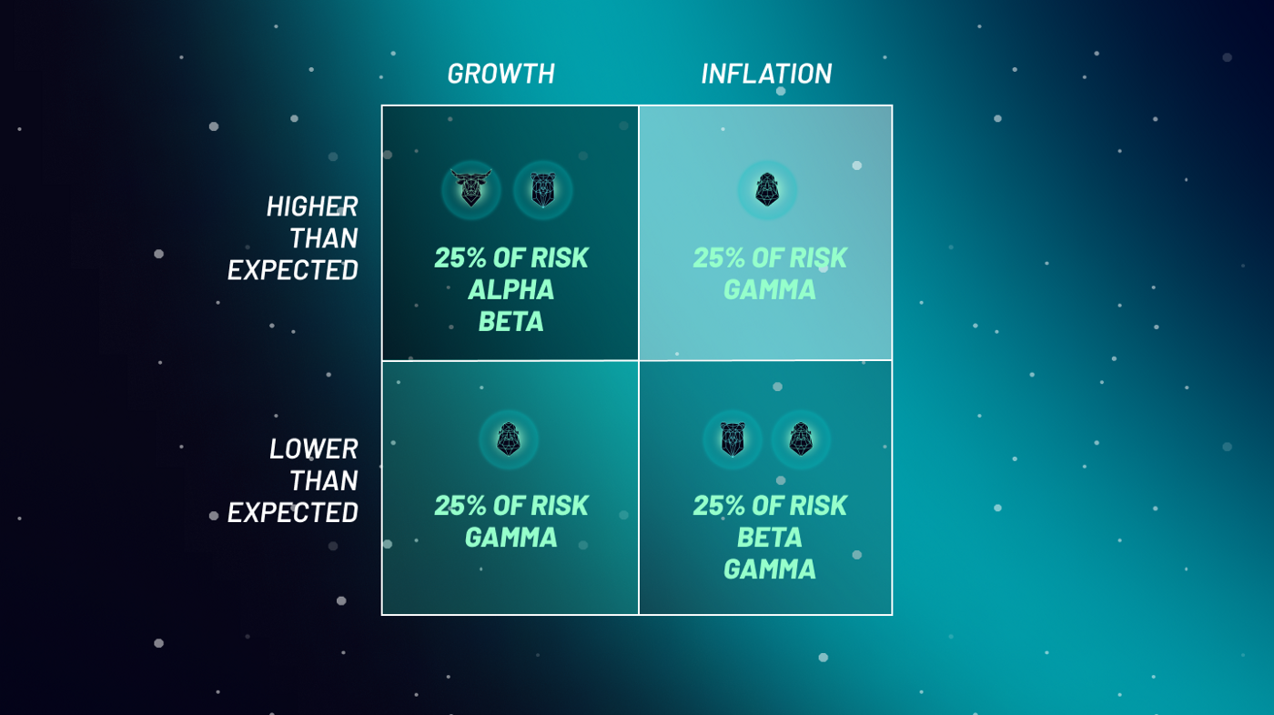
Figure 17: Portfolio Risk Concentrations

We will assign assets to each box - in Figure (16) - so that the amount of risk is the same for each box, whatever the returns from the box corresponding to the relevant market conditions. For instance in Figure (17), the dollar amount granted to Alpha assets will be lower than the appropriation to Gamma since Gamma assets are less risky. Investors can choose a desired level of risk - or equivalent to a target return - and the distribution of their funds to each of the boxes, to create a customized portfolio, will be done by the investment machinery we outline in this paper. This personalized portfolio - issued as a Parity index token on blockchain - will supply returns based upon the specific risk appetite of the investor, no matter the environment.

Though less likely, if growth and inflation meet expectations, that is a good problem to have. In this case, all four quadrants will perform satisfactorily and the combined portfolio will still meet the stated objectives.

6.2 Crypto Environmental Nuances

While economic growth can be considered a basic environmental factor for traditional assets, growth in the crypto universe can also be linked to two parallel dimensions related to: trustworthiness and benefits of transacting with a particular cryptocurrency as the medium of exchange. Trustworthiness is heavily dependent on the extent of computing power (or nodes)  deployed on a particular platform to verify transactions. The transaction benefits are proportional to size of the network or the number of active users (wallets) and how well accepted the particular currency. The allocation to the four boxes will have to balance out any fluctuations in the trends of these two key crypto-movers over time.

In conventional investing techniques, selection of assets to balance risks depends on their mutual correlations. Practical experience from managing portfolios shows that correlations are inherently unstable. Hence, as our models evolve, our approach to measuring alikeness will use metrics that capture higher dimensions of similarity (and variability) between assets by looking at attributes well beyond risk, return and correlations.

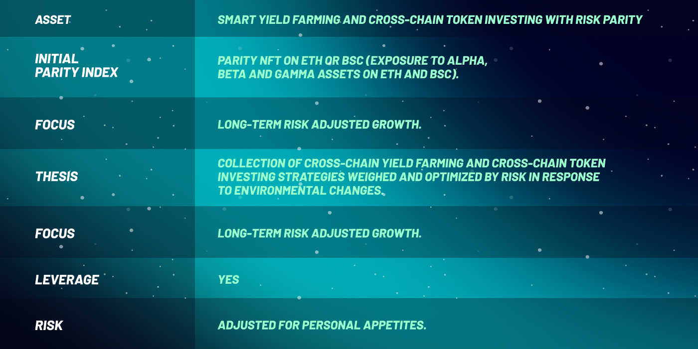
Figure 18: Risk Parity Highlights

The Parity indexes are composites of the Alpha, Beta and Gamma index classes, weighted so that the risk from each bucket is limited to 25% of the total. The final result is a individualized matrix of aggregated cross-chain tokens and yield farming strategies (Figure 18). It is algorithmically controlled by smart contracts, regularly rebalancing to keep optimal coverage and maintain the 25% ratio. It is possible that most investors might chose high risk - or low risk - as their preference. In this case, it would be difficult to allot equal weight to all the four environmental boxes in Figure (16) unless we limit the maximum risk - and hence the return - that can be obtained from the overall fund.

The online investing process captures the member’s individual risk appetite (directly or from their DeFi asset manager) and uses it to weight the cross-chain Alpha, Beta and Gamma assets appropriately. A Parity index token is then minted. It is personalized to the member’s needs, representing the best risk-adjusted De-Fi investment in the market. The Parity index token can itself then be staked, exchanged or traded without any limit for further gain.

6.3 Fortune Favors The Prepared Portfolio

Current views on investing hold many reservations regarding the use of Leverage. While excessive leverage can result in losses, a modest amount of leverage, when applied to a small portion of the overall portfolio, has many benefits. In conventional portfolios that are chasing a certain level of return, the majority of the holdings will be concentrated in assets that are closer to the benchmark in terms of their returns. The risk characteristics of these assets are derived from similar sources with the end result being that the overall portfolio will not be well diversified.

A moderate amount of leverage is included in the Parity index class due to the leverage within the Alpha index class. Our Alpha suite will have assets that aim for spectacular returns, but could have risks derived from similar fundamental properties. Hence, to mitigate the concentration risk, we will mix in assets possessing distinctive risk features. These non-identical assets could have lower return profiles, but when they are levered up and combined into the portfolio, they provide an excellent source of diverging movements that offset the overall risk.

This amplification of the returns from chosen assets results in an investment profile that can have lower risk than those of conventional portfolios, which concentrate their holding around assets with similar risk return configurations, providing the same level of returns. The use of leverage in the DeFi world can be seamless due to the high degree of automation. Smart contracts will monitor the level of leverage and automatically trigger events to offset extreme and adverse shifts.

6.4 Risk Management Is But Taming The Volatility Skew

The Parity portfolios carry a risk level adjusted to the needs of the member. Each Parity index token is personalized and minted with the appropriate weightings of Alpha, Beta and Gamma index class investments.

The most crucial aspect of asset management is to have a rigorous process to calculate risk.  Risk is defined and understood in several ways. It is also important to differentiate between risk and uncertainty, which we will explore in subsequent articles. We consider risk as an indicator of the extent of variation in the returns of assets. One of the commonly used metrics as a gauge for risk is the volatility. A particularly popular approach to volatility is computing the standard deviation of returns.

The main issue with minimizing risk using volatility is that volatility is an unobserved variable. This means volatility can only be estimated over historical periods or forecasted over future times since it cannot be directly seen. To mitigate this issue, our models will calculate asset weights based on a range of volatilities rather than trying to pin down one exact volatility number. The additional benefit from this approach will be reduced rebalancing efforts, which will decrease the corresponding blockchain gas costs.

A secondary drawback of volatility is that it fails to capture the effect of changes in the direction of any variable (Kashyap 2021). That is both rising or falling prices are treated equally and hence if we are long a security, upward movements in security prices could get penalized as excess volatility in portfolio management decisions. As an alternative, we devise a metric to measure the path taken by the variable to arrive at the current value, over the last few time periods. To articulate the intuition, any security that had steady upward growth, over a particular time period, is ranked higher than a security with similar growth, over the same time period but with more ups and downs in the path, or changes in direction. Assets are penalized for having ups and downs in their price process. But unidirectional upward jumps suffer no such penalty.

6.5 Sharpening the Sharpe Ratio

A key metric used to assess the performance of portfolios is known as the Sharpe Ratio (SR: Sharpe 1966; 1994; End-note 29). The ratio is the average return (historical or expected) earned on a portfolio in excess of the risk-free rate per unit of volatility or total risk. The widespread use of this metric can be explained due to its simplicity and the powerful insights it provides to investors in understanding how their goals related to risk and return are being met.

An important limitation of the SR is that averages and standard deviations are not enough to completely understand the randomness inherent in the returns generated by any asset. While this limitation is severe enough in traditional portfolios, it is all the more crucial in DeFi. Given the greater volatilities of crypto-assets there are well justified reasons to develop complementary techniques to measure portfolio performance. As a refinement of the SR, we will pay close attention to additional statistical properties called higher moments, also known as Skew and Kurtosis, which show whether there is a greater tendency for either positive or negative movement of returns and whether extreme events are more likely when compared to a normal distribution (Anson, Ho & Silberstein 2007; Grigoletto & Lisi 2011; Theodossiou & Savva 2016; End-notes 30; 31).

6.6 Investor Experience on Blockchain

The user experience has been designed such that investors can tailor their wealth allocations to their preferred risk appetites (Figure 15).  Users can select either their preferred level of risk or return. Investors can also directly decide how much of their wealth they want to allocate to the three funds: Alpha, Beta and Gamma. Once either of the three routes are selected, (Risk or Return or Weights of Alpha, Beta and Gamma), the other parameters are automatically calculated and saved into an NFT, which the investor will hold for the life of the investment.

The preferences can be changed anytime by investors and this will trigger a readjustment of their sub fund allocations. Our investment specialists will also monitor the markets and, as the relationship between risk and return changes, will fine tune the parameters of the parity line and update the parameters of the portfolio allocations. This will guarantee that all investors are getting the best possible outcomes customized for their desired wealth management objectives.

The challenge will be to ensure that the user interactions are intuitive, and yet their preferences are precisely captured in the investment decisions. This has been accomplished by letting someone who does not wish to be bothered with all the settings, or a novice investor, have the simple option of choosing the default, depositing his funds and forgetting about everything else. If this is the option chosen, the portfolio will select a low level of risk and calculate the other parameters accordingly. Advanced users can choose their risk level or their expected return, or the weights they want to assign to each of the sub funds. The other parameters will be automatically calculated based on the discussion in Section (5).

The outcome of these innovations is an investment machinery that responds to investor preferences and adapts to changing market conditions.  All of this can be viewed as a natural progression from the conventional efficient frontier to a progressive final frontier, which will continue to transcend itself.

6.7 Parity Fees

The following points capture the main fee structure for Parity investors. Levying some kind of fees is the way in which investment funds - for example: hedge funds, mutual funds, ETFs - cover their costs and make profits (Golec 1996; Elton, Gruber & Blake 2003; Guasoni & Obłój 2016; Khorana et al., 2009; End-notes 37; 35; 36; 38). In the blockchain environment the investment fund has additional costs related to performing transactions on the network.

We wish to highlight that there is a separate component that will share a percentage of the profits - levied from the fees - with the investors to ensure wealth management firms stay true to the spirit of decentralization (Singh & Kim 2019; Wang et al., 2019; Santana & Albareda 2022; Barbereau & Bodó 2023; Rikken et al., 2023; Kashyap 2022; 2023; End-note 33). All the fee rates, time and other variables - the sample values shown below are based on what we have used in various investment scenarios - should be configurable unless otherwise specified.

1. Parity investors can be charged a deposit fees as a percentage of the amount being deposited.

2. Whenever the user changes their preferences, and updates their corresponding NFT, a percentage fees proportional to the total deposited amount can also be levied. The user preferences change fees should be capped at a certain maximum amount.

3. Whenever a new amount is deposited, the minimum of the fee component for deposits or the fee amount for user preference changes can be levied (Points 1; 2). It is possible to separate the deposit action and the user preference action in which case the deposit fees and user preference fees can be set to be different depending on the network gas fees, fund expenses and other factors (Zarir et a., 2021; Donmez & Karaivanov 2022; Laurent et al., 2022; Kashyap 2023; End-note 32).

4. The withdraw fees or the redemption penalty for Parity can be in three tiers for three different holding time periods. The redemption penalty rates and the corresponding time periods should be configurable. We provide the below only as a numerical example. Since these values have to be configured depending on various considerations.

   1. 5% early redemption penalty for investing less than 30 days.

   2. 4% early redemption penalty for investing between 30 to 60 days.

   3. 3% early redemption penalty for investing between 60 to 90 days.

   4. No redemption penalty for investing more than 90 days.

5. There is no lockout period - a minimum investment period - for Parity unlike Alpha, Beta and Gamma. There should be no lockout period for Parity when it invests in Alpha, Beta and Gamma. The lockout periods for Alpha, Beta and Gamma should be comparable to the no redemption penalty time horizon for Parity.

6. Parity will be charged different deposit fee rates for investing into Alpha, Beta and Gamma as compared to other investors who might invest directly into Alpha, Beta and Gamma. This will allow investors who invest into Parity rather than investing directly into Alpha, Beta and Gamma to benefit from lower total fees. For example right now, the Alpha deposit rate is 0.5%. We would then have a different Parity Alpha deposit rate, such as 0.3%. This 0.3% is an example only and a provision has to made to so that it can be changed from a suitable GUI by the administrators of the investment platform. Setting the actual rates rather than setting a discount rate provides more flexibility and the rate can also be made zero at times, which is impossible with a discount rate.

7. The fees that Parity gets charged when investing into Alpha, Beta and Gamma will then become a cost for Parity accordingly. Any benefits from netting within Parity then adds to the profits generated by Parity and will be sent to the corresponding treasury, which will be a separate wallet or smart contract.

7 Conclusion: The Blockchain Revolution For Wealth Gains Without The Pains

We have created several novel techniques to bring many mechanisms that have worked well in the traditional financial wealth management arena to the blockchain space. We have given detailed algorithmic steps to help with technical implementation of the methodologies we have developed.

We have discussed how to overcome several issues with the efficient frontier. We have pioneered several solutions designed not only to bring risk parity to the blockchain environment, but also provided ways in which the efficient set of assets can continue to evolve - becoming the final frontier of wealth management.

Risk Parity investing for cross chain DeFi will be a new development in decentralized investing. Members receive a personalized balanced cross chain portfolio constructed algorithmically according to the Risk Parity strategy. It includes varying measures of three funds - index exposures to Alpha, Beta and Gamma, which have varying risk profiles - risk-adjusted to the requirements of each investor. It is engineered to provide long term high yields protected from market downturns and environmental shocks.

The innovations we have designed to realize risk parity on blockchain also address techniques to combine the efficient frontier with equal risk allocation to the assets within a portfolio. We have termed these set of concepts: “conceptual parity” and detailed elaborate methods to simplify its implementation in decentralized technology using the notion of what we have descried as the “Parity Line”.

We have given detailed mathematical formulations, and technical pointers, to be able to implement the mechanisms we have created as blockchain smart contracts. Our approach overcomes numerous blockchain bottlenecks and takes the power of smart contracts much further. The numerical illustrations we have given depict various scenarios regarding risk return combinations - of Alpha, Beta and Gamma - to obtain parity portfolios on blockchain.

The fundamental doctrine of DeFi is equal access and rights to all participants coupled with complete freedom from any central controlling authority. Bringing this notion of equality to investing is the core impetus behind initiating the risk parity movement in DeFi. This translates to providing sophisticated asset management - with risk mitigation - techniques, insights and wealth appreciation schemes to all investors. To become trailblazer ’s on this voyage, is doing the needful - and implementing some of the ideas discussed in this paper - so that accumulating a Fortune is just a mouse click away from everyone.

Mutual funds, hedge funds and other traditional investments have had a significant impact in the lives of many individuals across the world. Despite their popularity, there are many concerns regarding their transparency and ease of access for everyone. Blockchain technology is extremely well suited to mitigate, if not entirely eliminate, those concerns. Decentralized ledger concepts and the technological advancements over the last several decades allow us to combine the best features of both traditional investment vehicles and the universal accessibility of blockchain.

Equal Wealth Generation Opportunities are Finally Here.

8 References

• Acharya, V. V., & Richardson, M. P. (Eds.). (2009). Restoring financial stability: how to repair a failed system (Vol. 542). John Wiley & Sons.

• Ambachtsheer, K. P. (1987). Pension fund asset allocation: In defense of a 60/40 equity/debt asset mix. Financial Analysts Journal, 43(5), 14-24.

• Ammann, M., Coqueret, G., & Schade, J. P. (2016). Characteristics-based portfolio choice with leverage constraints. Journal of Banking & Finance, 70, 23-37.

• Anderson, R. M., Bianchi, S. W., & Goldberg, L. R. (2012). Will my risk parity strategy outperform?. Financial Analysts Journal, 68(6), 75-93.

• Anson, M., Ho, H., & Silberstein, K. (2007). Building a hedge fund portfolio with kurtosis and skewness. The Journal of Alternative Investments, 10(1), 25.

• Ante, L., Fiedler, I., & Strehle, E. (2021). The influence of stablecoin issuances on cryptocurrency markets. Finance Research Letters, 41, 101867.

• Asness, C. S., Frazzini, A., & Pedersen, L. H. (2012). Leverage aversion and risk parity. Financial Analysts Journal, 68(1), 47-59.

• Ballestero, E. (2005). Mean-semivariance efficient frontier: a downside risk model for portfolio selection. Applied Mathematical Finance, 12(1), 1-15.

• Baldry, C. (1999). Space-the final frontier. Sociology, 33(3), 535-553.

• Bai, X., Scheinberg, K., & Tutuncu, R. (2016). Least-squares approach to risk parity in portfolio selection. Quantitative Finance, 16(3), 357-376.

• Bao, H., & Roubaud, D. (2022). Non-fungible token: A systematic review and research agenda. Journal of Risk and Financial Management, 15(5), 215.

• Barbereau, T., & Bodó, B. (2023). Beyond financial regulation of crypto-asset wallet software: In search of secondary liability. Computer Law & Security Review, 49, 105829.

• Barberis, N., & Thaler, R. (2003). A survey of behavioral finance. Handbook of the Economics of Finance, 1, 1053-1128.

• Bellini, Fabio, Francesco Cesarone, Christian Colombo, and Fabio Tardella. "Risk parity with expectiles." European journal of operational research 291, no. 3 (2021): 1149-1163.

• Bender, J., Briand, R., Nielsen, F., & Stefek, D. (2010). Portfolio of risk premia: A new approach to diversification. The Journal of Portfolio Management, 36(2), 17-25.

• Bertsekas, D. (2009). Convex optimization theory (Vol. 1). Athena Scientific.

• Bertsekas, D. (2015). Convex optimization algorithms. Athena Scientific.

• Best, M. J., & Hlouskova, J. (2000). The efficient frontier for bounded assets. Mathematical methods of operations research, 52, 195-212.

• Bhansali, V. (2011). Beyond risk parity. The Journal of Investing, 20(1), 137-147.

• Bi, J., Jin, H., & Meng, Q. (2018). Behavioral mean-variance portfolio selection. European Journal of Operational Research, 271(2), 644-663.

• Black, F., & Litterman, R. (1992). Global portfolio optimization. Financial analysts journal, 48(5), 28-43.

• Bolstad, W. M., & Curran, J. M. (2016). Introduction to Bayesian statistics. John Wiley & Sons.

• Bond, S. A., & Satchell, S. E. (2002). Statistical properties of the sample semi-variance. Applied Mathematical Finance, 9(4), 219-239.

• Boyd, S. P., & Vandenberghe, L. (2004). Convex optimization. Cambridge university press.

• Braga, M. D., Nava, C. R., & Zoia, M. G. (2023). Kurtosis-based risk parity: methodology and portfolio effects. Quantitative Finance, 23(3), 453-469.

• Britten-Jones, M. (1999). The sampling error in estimates of mean-variance efficient portfolio weights. The Journal of Finance, 54(2), 655-671.

• Brode, D., & Brode, S. T. (Eds.). (2015). The Star Trek Universe: Franchising the Final Frontier. Rowman & Littlefield.

• Buttell, A. E. (2010). Harry M. Markowitz on modern portfolio theory, the efficient frontier, and His Life’s Work. Journal of Financial Planning, 23(5), 18.

• Calvo, C., Ivorra, C., & Liern, V. (2012). On the computation of the efficient frontier of the portfolio selection problem. Journal of Applied Mathematics, 2012.

• Calvo, C., Ivorra, C., & Liern, V. (2016). Fuzzy portfolio selection with non-financial goals: exploring the efficient frontier. Annals of Operations Research, 245(1-2), 31-46.

• Camerer, C. (1999). Behavioral economics: Reunifying psychology and economics. Proceedings of the National Academy of Sciences, 96(19), 10575-10577.

• Chaves, D., Hsu, J., Li, F., & Shakernia, O. (2011). Risk parity portfolio vs. other asset allocation heuristic portfolios. Journal of Investing, 20(1), 108.

• Chen, L., He, S., & Zhang, S. (2011). Tight bounds for some risk measures, with applications to robust portfolio selection. Operations Research, 59(4), 847-865.

• Christodoulakis, G. A. (2002). Bayesian optimal portfolio selection: the black-litterman approach. Unpublished paper.

• Ciotti, M., Ciccozzi, M., Terrinoni, A., Jiang, W. C., Wang, C. B., & Bernardini, S. (2020). The COVID-19 pandemic. Critical reviews in clinical laboratory sciences, 57(6), 365-388.

• Clarke, R., De Silva, H., & Thorley, S. (2013). Risk parity, maximum diversification, and minimum variance: An analytic perspective. The Journal of Portfolio Management, 39(3), 39-53.

• Cochrane, J. (2009). Asset pricing: Revised edition. Princeton university press.

• Cohen, K. J., & Pogue, J. A. (1967). An empirical evaluation of alternative portfolio-selection models. The Journal of Business, 40(2), 166-193.

• Constantinides, G. M., & Malliaris, A. G. (1995). Portfolio theory. Handbooks in operations research and management science, 9, 1-30.

• Cook, S. (2000). The P versus NP problem. Clay Mathematics Institute, 2.

• Dannen, C. (2017). Introducing Ethereum and solidity (Vol. 1, pp. 159-160). Berkeley: Apress.

• Da Silva, A. S., Lee, W., & Pornrojnangkool, B. (2009). The Black–Litterman model for active portfolio management. The Journal of Portfolio Management, 35(2), 61-70.

• De Souza, C., & Smirnov, M. (2004). Dynamic leverage. Journal of Portfolio Management, 31, 25-39.

• Donmez, A., & Karaivanov, A. (2022). Transaction fee economics in the Ethereum blockchain. Economic Inquiry, 60(1), 265-292.

• Drobetz, W. (2001). How to avoid the pitfalls in portfolio optimization? Putting the Black-Litterman approach at work. Financial Markets and Portfolio Management, 15(1), 59.

• Dromey, R. G. (1982). How to Solve it by Computer. Prentice-Hall, Inc..

• Dubois, D., & Prade, H. (2001). Possibility theory, probability theory and multiple-valued logics: A clarification. Annals of mathematics and Artificial Intelligence, 32, 35-66.

• Dubois, D. (2006). Possibility theory and statistical reasoning. Computational statistics & data analysis, 51(1), 47-69.

• Duffie, D., & Pan, J. (1997). An overview of value at risk. Journal of derivatives, 4(3), 7-49.

• Elton, E. J., & Gruber, M. J. (1973). Estimating the dependence structure of share prices–implications for portfolio selection. The Journal of Finance, 28(5), 1203-1232.

• Elton, E. J., Gruber, M. J., & Padberg, M. W. (1976). Simple criteria for optimal portfolio selection. The Journal of finance, 31(5), 1341-1357.

• Elton, E. J., Gruber, M. J., & Padberg, M. W. (1977a). Simple criteria for optimal portfolio selection with upper bounds. Operations Research, 25(6), 952-967.

• Elton, E. J., Gruber, M. J., & Padberg, M. W. (1977b). Simple rules for optimal portfolio selection: the multi group case. Journal of Financial and Quantitative Analysis, 12(3), 329-345.

• Elton, E. J., Gruber, M. J., & Padberg, M. W. (1978). Simple criteria for optimal portfolio selection: tracing out the efficient frontier. The Journal of Finance, 33(1), 296-302.

• Elton, E. J., Gruber, M. J., & Padberg, M. W. (1979). Simple criteria for optimal portfolio selection: the multi-index case. Portfolio theory, 25, 7-19.

• Elton, E. J., & Gruber, M. J. (1997). Modern portfolio theory, 1950 to date. Journal of banking & finance, 21(11-12), 1743-1759.

• Elton, E. J., Gruber, M. J., & Blake, C. R. (2003). Incentive fees and mutual funds. The Journal of Finance, 58(2), 779-804.

• Elton, E. J., Gruber, M. J., Brown, S. J., & Goetzmann, W. N. (2009). Modern portfolio theory and investment analysis. John Wiley & Sons.

• Fan, X., Niu, B., & Liu, Z. (2022). Scalable blockchain storage systems: research progress and models. Computing, 104(6), 1497-1524.

• Fabozzi, F. J., Gupta, F., & Markowitz, H. M. (2002). The legacy of modern portfolio theory. The journal of investing, 11(3), 7-22.

• Fabozzi, F. A., Simonian, J., & Fabozzi, F. J. (2021). Risk parity: The democratization of risk in asset allocation. The Journal of Portfolio Management, 47(5), 41-50.

• Fama, E. F., & MacBeth, J. D. (1973). Risk, return, and equilibrium: Empirical tests. Journal of political economy, 81(3), 607-636.

• Fama, E. F., & French, K. R. (2004). The capital asset pricing model: Theory and evidence. Journal of economic perspectives, 18(3), 25-46.

• Fernández, A., & Gómez, S. (2007). Portfolio selection using neural networks. Computers & operations research, 34(4), 1177-1191.

• Fisher, G. S., Maymin, P. Z., & Maymin, Z. G. (2015). Risk parity optimality. The Journal of Portfolio Management, 41(2), 42-56.

• Fortnow, L. (2009). The status of the P versus NP problem. Communications of the ACM, 52(9), 78-86.

• Frahm, G., & Wiechers, C. (2011). On the diversification of portfolios of risky assets (No. 2/11). Discussion Papers in Statistics and Econometrics.

• Frost, P. A., & Savarino, J. E. (1986). An empirical Bayes approach to efficient portfolio selection. Journal of Financial and Quantitative Analysis, 21(3), 293-305.

• Garas, A., Argyrakis, P., & Havlin, S. (2008). The structural role of weak and strong links in a financial market network. The European Physical Journal B, 63, 265-271.

• Garvey, R., & Murphy, A. (2005). Entry, exit and trading profits: A look at the trading strategies of a proprietary trading team. Journal of Empirical Finance, 12(5), 629-649.

• Gelman, A., & Shalizi, C. R. (2013). Philosophy and the practice of Bayesian statistics. British Journal of Mathematical and Statistical Psychology, 66(1), 8-38.

• Goldfarb, D., & Iyengar, G. (2003). Robust portfolio selection problems. Mathematics of operations research, 28(1), 1-38.

• Golec, J. H. (1996). The effects of mutual fund managers’ characteristics on their portfolio performance, risk and fees. Financial Services Review, 5(2), 133-147.

• Green, R. C., & Hollifield, B. (1992). When will mean-variance efficient portfolios be well diversified?. The Journal of Finance, 47(5), 1785-1809.

• Grigoletto, M., & Lisi, F. (2011). Practical implications of higher moments in risk management. Statistical Methods & Applications, 20, 487-506.

• Grobys, K., Junttila, J., Kolari, J. W., & Sapkota, N. (2021). On the stability of stablecoins. Journal of Empirical Finance, 64, 207-223.

• Gunjan, A., & Bhattacharyya, S. (2023). A brief review of portfolio optimization techniques. Artificial Intelligence Review, 56(5), 3847-3886.

• Guasoni, P., & Obłój, J. (2016). The incentives of hedge fund fees and high-water marks. Mathematical Finance, 26(2), 269-295.

• Harvey, C. R., Hoyle, E., Korgaonkar, R., Rattray, S., Sargaison, M., & Van Hemert, O. (2018). The impact of volatility targeting. The Journal of Portfolio Management, 45(1), 14-33.

• Harvey, C. R., Ramachandran, A., & Santoro, J. (2021). DeFi and the Future of Finance. John Wiley & Sons.

• He, G., & Litterman, R. (2002). The intuition behind Black-Litterman model portfolios. Available at SSRN 334304.

• Hirshleifer, D. (2015). Behavioral finance. Annual Review of Financial Economics, 7, 133-159.

• Hoang, L. T., & Baur, D. G. (2021). How stable are stablecoins?. The European Journal of Finance, 1-17.

• Huang, X. (2006). Fuzzy chance-constrained portfolio selection. Applied mathematics and computation, 177(2), 500-507.

• Huang, X. (2007a). Portfolio selection with fuzzy returns. Journal of Intelligent & Fuzzy Systems, 18(4), 383-390.

• Huang, X. (2007b). Two new models for portfolio selection with stochastic returns taking fuzzy information. European Journal of Operational Research, 180(1), 396-405.

• Huang, X. (2008a). Risk curve and fuzzy portfolio selection. Computers & mathematics with applications, 55(6), 1102-1112.

• Huang, X. (2008b). Portfolio selection with a new definition of risk. European Journal of operational research, 186(1), 351-357.

• Huberts, L. C. (2004). Overlay Speak. The Journal of Investing, 13(3), 22-30.

• Hull, J. C. (2003). Options futures and other derivatives. Pearson Education India.

• Hursh, S. R. (1984). Behavioral economics. Journal of the experimental analysis of behavior, 42(3), 435-452.

• Jacobs, B. I., & Levy, K. N. (2012). Leverage aversion and portfolio optimality. Financial Analysts Journal, 68(5), 89-94.

• Jolliffe, I. T., & Cadima, J. (2016). Principal component analysis: a review and recent developments. Philosophical transactions of the royal society A: Mathematical, Physical and Engineering Sciences, 374(2065), 20150202.

• Jorion, P. (1996). Risk2: Measuring the risk in value at risk. Financial analysts journal, 52(6), 47-56.

• Jorion, P. (2007). Value at risk: the new benchmark for managing financial risk. McGraw-Hill.

• Kalymon, B. A. (1971). Estimation risk in the portfolio selection model. Journal of Financial and Quantitative Analysis, 6(1), 559-582.

• Kashyap, R. (2021). Behavioural Bias Benefits: Beating Benchmarks By Bundling Bouncy Baskets. Accounting & Finance, 61(3), 4885-4921.

• Kashyap, R. (2022). Bringing Risk Parity To The DeFi Party: A Complete Solution To The Crypto Asset Management Conundrum. Working Paper.

• Kashyap, R. (2023). The Democratization of Wealth Management: Hedged Mutual Fund Blockchain Protocol. Available at SSRN 4543339.

• Khorana, A., Servaes, H., & Tufano, P. (2009). Mutual fund fees around the world. The Review of Financial Studies, 22(3), 1279-1310.

• Kim, J. H., Lee, Y., Kim, W. C., & Fabozzi, F. J. (2021). Mean–variance optimization for asset allocation. The Journal of Portfolio Management, 47(5), 24-40.

• Kocheturov, A., Batsyn, M., & Pardalos, P. M. (2014). Dynamics of cluster structures in a financial market network. Physica A: Statistical Mechanics and its Applications, 413, 523-533.

• Konstantinov, G. S. (2021). What Portfolio in Europe Makes Sense?. The Journal of Portfolio Management.

• Kroll, Y., Levy, H., & Rapoport, A. (1988). Experimental tests of the mean-variance model for portfolio selection. Organizational Behavior and Human Decision Processes, 42(3), 388-410.

• Krugman, P. (1998). Space: the final frontier. Journal of Economic perspectives, 12(2), 161-174.

• Kugler, L. (2021). Non-fungible tokens and the future of art. Communications of the ACM, 64(9), 19-20.

• Kurt Peker, Y., Rodriguez, X., Ericsson, J., Lee, S. J., & Perez, A. J. (2020). A cost analysis of internet of things sensor data storage on blockchain via smart contracts. Electronics, 9(2), 244.

• Kwakernaak, H. (1978). Fuzzy random variables—I. Definitions and theorems. Information sciences, 15(1), 1-29.

• Laurent, A., Brotcorne, L., & Fortz, B. (2022). Transaction fees optimization in the Ethereum blockchain. Blockchain: Research and Applications, 3(3), 100074.

• Ledoit, O., & Wolf, M. (2003). Improved estimation of the covariance matrix of stock returns with an application to portfolio selection. Journal of empirical finance, 10(5), 603-621.

• Leland, H. E. (1999). Beyond mean–variance: Performance measurement in a nonsymmetrical world (corrected). Financial analysts journal, 55(1), 27-36.

• Li, B., & Hoi, S. C. (2014). Online portfolio selection: A survey. ACM Computing Surveys (CSUR), 46(3), 1-36.

• Li, B., Hoi, S. C., Sahoo, D., & Liu, Z. Y. (2015). Moving average reversion strategy for on-line portfolio selection. Artificial Intelligence, 222, 104-123.

• Lindley, D. V. (1972). Bayesian statistics: A review. Society for industrial and applied mathematics.

• Liu, Y. J., & Zhang, W. G. (2013). Fuzzy portfolio optimization model under real constraints. Insurance: Mathematics and Economics, 53(3), 704-711.

• Lohre, H., Neugebauer, U., & Zimmer, C. (2012). Diversified risk parity strategies for equity portfolio selection. The Journal of Investing, 21(3), 111-128.

• Lohre, H., Opfer, H., & Orszag, G. (2014). Diversifying risk parity. Journal of Risk, 16(5), 53-79.

• Loney, S. L. (1897). The elements of coordinate geometry. Macmillan and Company.

• Lyons, R. K., & Viswanath-Natraj, G. (2023). What keeps stablecoins stable?. Journal of International Money and Finance, 131, 102777.

• Madan, D. B., & Sharaiha, Y. M. (2015). Option overlay strategies. Quantitative Finance, 15(7), 1175-1190.

• Maillard, S., Roncalli, T., & Teïletche, J. (2010). The properties of equally weighted risk contribution portfolios. The Journal of Portfolio Management, 36(4), 60-70.

• Mao, J. C., & Särndal, C. E. (1966). A decision theory approach to portfolio selection. Management Science, 12(8), B-323.

• Markowitz, H. M. (1952). Portfolio selection. Journal of Finance 7 (1), 77-91.

• Markowitz, H. M. (1959). Portfolio Selection: Efficient Diversification of Investments. Cowles Foundation Monograph 16, New York: John Wiley & Sons.

• Martinez, W. L. (2011). Graphical user interfaces. Wiley Interdisciplinary Reviews: Computational Statistics, 3(2), 119-133.

• Meucci, A. (2009). Managing diversification. Risk, 74-79.

• McNeil, A. J., Frey, R., & Embrechts, P. (2015). Quantitative risk management: concepts, techniques and tools-revised edition. Princeton university press.

• Merton, R. C. (1972). An analytic derivation of the efficient portfolio frontier. Journal of financial and quantitative analysis, 7(4), 1851-1872.

• Michaud, R. O. (1989). The Markowitz optimization enigma: Is ‘optimized’optimal?. Financial analysts journal, 45(1), 31-42.

• Mohanty, S. S., Mohanty, O., & Ivanof, M. (2021). Alpha enhancement in global equity markets with ESG overlay on factor-based investment strategies. Risk Management, 23(3), 213-242.

• Momen, O., Esfahanipour, A., & Seifi, A. (2019). Collective mental accounting: an integrated behavioural portfolio selection model for multiple mental accounts. Quantitative Finance, 19(2), 265-275.

• Momen, O., Esfahanipour, A., & Seifi, A. (2020). A robust behavioral portfolio selection: model with investor attitudes and biases. Operational Research, 20, 427-446.

• Monrat, A. A., Schelén, O., & Andersson, K. (2019). A survey of blockchain from the perspectives of applications, challenges, and opportunities. IEEE Access, 7, 117134-117151.

• Mullainathan, S., & Thaler, R. H. (2000). Behavioral Economics (No. 7948). National Bureau of Economic Research, Inc.

• Mulvey, J. M., Ural, C., & Zhang, Z. (2007). Improving performance for long-term investors: wide diversification, leverage, and overlay strategies. Quantitative Finance, 7(2), 175-187.

• Murty, K. G., & Kabadi, S. N. (1985). Some NP-complete problems in quadratic and nonlinear programming.

• Nahmias, S. (1978). Fuzzy variables. Fuzzy sets and systems, 1(2), 97-110.

• Nakamoto, S. (2008). Bitcoin: A peer-to-peer electronic cash system. Decentralized Business Review, 21260.

• Namaki, A., Shirazi, A. H., Raei, R., & Jafari, G. R. (2011). Network analysis of a financial market based on genuine correlation and threshold method. Physica A: Statistical Mechanics and its Applications, 390(21-22), 3835-3841.

• Nantell, T. J., & Price, B. (1979). An analytical comparison of variance and semivariance capital market theories. Journal of Financial and Quantitative Analysis, 14(2), 221-242.

• Narayanan, A., & Clark, J. (2017). Bitcoin’s academic pedigree. Communications of the ACM, 60(12), 36-45.

• Nuti, G., Mirghaemi, M., Treleaven, P., & Yingsaeree, C. (2011). Algorithmic trading. Computer, 44(11), 61-69.

• Palczewski, A., & Palczewski, J. (2014). Theoretical and empirical estimates of mean–variance portfolio sensitivity. European Journal of Operational Research, 234(2), 402-410.

• Pardo, R. (2011). The evaluation and optimization of trading strategies. John Wiley & Sons.

• Pástor, Ľ. (2000). Portfolio selection and asset pricing models. The Journal of Finance, 55(1), 179-223.

• Pearson, R., & Davies, M. M. (2014). Star Trek and American Television. Univ of California Press.

• Penman, S. H. (1970). What Net Asset Value?–An Extension of a Familiar Debate. The Accounting Review, 45(2), 333-346.

• Peralta, G., & Zareei, A. (2016). A network approach to portfolio selection. Journal of Empirical Finance, 38, 157-180.

• Pierro, G. A., & Tonelli, R. (2022, March). Can Solana be the solution to the blockchain scalability problem?. In 2022 IEEE International Conference on Software Analysis, Evolution and Reengineering (SANER) (pp. 1219-1226). IEEE.

• Piñeiro-Chousa, J., López-Cabarcos, M. Á., Sevic, A., & González-López, I. (2022). A preliminary assessment of the performance of DeFi cryptocurrencies in relation to other financial assets, volatility, and user-generated content. Technological Forecasting and Social Change, 181, 121740.

• Pogue, G. A. (1970). An extension of the Markowitz portfolio selection model to include variable transactions’ costs, short sales, leverage policies and taxes. The Journal of Finance, 25(5), 1005-1027.

• Polson, N. G., & Tew, B. V. (2000). Bayesian portfolio selection: An empirical analysis of the S&P 500 index 1970–1996. Journal of Business & Economic Statistics, 18(2), 164-173.

• Prince, B. (2011). Risk Parity Is About Balance. Bridgewater Associates, LP.

• Qian, E. (2011). Risk parity and diversification. The Journal of Investing, 20(1), 119-127.

• Qian, E. (2013). Are risk-parity managers at risk parity?. The Journal of Portfolio Management, 40(1), 20-26.

• Qian, J. (2015). An introduction to asset pricing theory.

• Rapach, D., & Zhou, G. (2013). Forecasting stock returns. In Handbook of economic forecasting (Vol. 2, pp. 328-383). Elsevier.

• Reinhart, C. M., & Rogoff, K. S. (2008). This time is different: A panoramic view of eight centuries of financial crises (No. w13882). National Bureau of Economic Research.

• Rikken, O., Janssen, M., & Kwee, Z. (2023). The ins and outs of decentralized autonomous organizations (DAOs) unraveling the definitions, characteristics, and emerging developments of DAOs. Blockchain: Research and Applications, 100143.

• Ritter, J. R. (2003). Behavioral finance. Pacific-Basin finance journal, 11(4), 429-437.

• Roncalli, T. (2013). Introduction to risk parity and budgeting. CRC Press.

• Roncalli, T., & Weisang, G. (2016). Risk parity portfolios with risk factors. Quantitative Finance, 16(3), 377-388.

• Rosenthal, J. S. (2006). First Look At Rigorous Probability Theory, A. World Scientific Publishing Company.

• Rubinstein, M. (2002). Markowitz’s" portfolio selection": A fifty-year retrospective. The Journal of finance, 57(3), 1041-1045.

• Rudin, W. (1953). Principles of mathematical analysis.

• Sahni, S. (1974). Computationally related problems. SIAM Journal on computing, 3(4), 262-279.

• Santana, C., & Albareda, L. (2022). Blockchain and the emergence of Decentralized Autonomous Organizations (DAOs): An integrative model and research agenda. Technological Forecasting and Social Change, 182, 121806.

• Schlecht, L., Schneider, S., & Buchwald, A. (2021). The prospective value creation potential of Blockchain in business models: A delphi study. Technological Forecasting and Social Change, 166, 120601.

• Schuhmacher, F., Kohrs, H., & Auer, B. R. (2021). Justifying mean-variance portfolio selection when asset returns are skewed. Management Science, 67(12), 7812-7824.

• Sharpe, W. F. (1966). Mutual fund performance. The Journal of business, 39(1), 119-138.

• Sharpe, W. F. (1994). The sharpe ratio. Journal of portfolio management, 21(1), 49-58.

• Shlens, J. (2014). A tutorial on principal component analysis. arXiv preprint arXiv:1404.1100.

• Singh, M., & Kim, S. (2019). Blockchain technology for decentralized autonomous organizations. In Advances in computers (Vol. 115, pp. 115-140). Elsevier.

• Sipser, M. (2006). Introduction to the Theory of Computation (Vol. 2). Boston: Thomson Course Technology.

• Tapscott, D., & Tapscott, A. (2016). Blockchain revolution: how the technology behind bitcoin is changing money, business, and the world. Penguin.

• Thaler, R. H. (1999). The end of behavioral finance. Financial Analysts Journal, 55(6), 12-17.

• Thaler, R. H. (2016). Behavioral economics: Past, present, and future. American economic review, 106(7), 1577-1600.

• Thaler, R. H. (2017). Behavioral economics. Journal of Political Economy, 125(6), 1799-1805.

• Theodossiou, P., & Savva, C. S. (2016). Skewness and the relation between risk and return. Management Science, 62(6), 1598-1609.

• Thiagarajan, S. R., & Schachter, B. (2011). Risk parity: Rewards, risks, and research opportunities. The Journal of Investing, 20(1), 79-89.

• Timmermann, A. (2008). Elusive return predictability. International Journal of Forecasting, 24(1), 1-18.

• Tomer, J. F. (2007). What is behavioral economics?. The Journal of Socio-Economics, 36(3), 463-479.

• Treynor, J. L., & Black, F. (1973). How to use security analysis to improve portfolio selection. The journal of business, 46(1), 66-86.

• Tsao, C. Y. (2010). Portfolio selection based on the mean–VaR efficient frontier. Quantitative Finance, 10(8), 931-945.

• van de Schoot, R., Depaoli, S., King, R., Kramer, B., Märtens, K., Tadesse, M. G., … & Yau, C. (2021). Bayesian statistics and modelling. Nature Reviews Methods Primers, 1(1), 1.

• Wang, S., Ding, W., Li, J., Yuan, Y., Ouyang, L., & Wang, F. Y. (2019). Decentralized autonomous organizations: Concept, model, and applications. IEEE Transactions on Computational Social Systems, 6(5), 870-878.

• Wang, Q., Li, R., Wang, Q., & Chen, S. (2021). Non-fungible token (NFT): Overview, evaluation, opportunities and challenges. arXiv preprint arXiv:2105.07447.

• Wood, G. (2014). Ethereum: A secure decentralised generalised transaction ledger. Ethereum project yellow paper, 151(2014), 1-32.

• Wu, H., Cao, J., Yang, Y., Tung, C. L., Jiang, S., Tang, B., … & Deng, Y. (2019, July). Data management in supply chain using blockchain: Challenges and a case study. In 2019 28th International Conference on Computer Communication and Networks (ICCCN) (pp. 1-8). IEEE.

• Xu, J., & Feng, Y. (2022). Reap the Harvest on Blockchain: A Survey of Yield Farming Protocols. IEEE Transactions on Network and Service Management.

• Yan, W., Miao, R., & Li, S. (2007). Multi-period semi-variance portfolio selection: Model and numerical solution. Applied Mathematics and Computation, 194(1), 128-134.

• Zadeh, L. A. (1965). Fuzzy sets. Information and control, 8(3), 338-353.

• Zadeh, L. A. (1978). Fuzzy sets as a basis for a theory of possibility. Fuzzy sets and systems, 1(1), 3-28.

• Zarir, A. A., Oliva, G. A., Jiang, Z. M., & Hassan, A. E. (2021). Developing cost-effective blockchain-powered applications: A case study of the gas usage of smart contract transactions in the ethereum blockchain platform. ACM Transactions on Software Engineering and Methodology (TOSEM), 30(3), 1-38.

• Zetzsche, D. A., Arner, D. W., & Buckley, R. P. (2020). Decentralized finance (defi). Journal of Financial Regulation, 6, 172-203.

• Zhang, W. G., Wang, Y. L., Chen, Z. P., & Nie, Z. K. (2007). Possibilistic mean–variance models and efficient frontiers for portfolio selection problem. Information Sciences, 177(13), 2787-2801.

• Zhang, W. G., & Wang, Y. L. (2008). An analytic derivation of admissible efficient frontier with borrowing. European Journal of Operational Research, 184(1), 229-243.

• Zhang, Y., Li, X., & Guo, S. (2018). Portfolio selection problems with Markowitz’s mean–variance framework: a review of literature. Fuzzy Optimization and Decision Making, 17, 125-158.

• Zhao, D., Bai, L., Fang, Y., & Wang, S. (2022). Multi-period portfolio selection with investor views based on scenario tree. Applied Mathematics and Computation, 418, 126813.

• Zheng, Z., Xie, S., Dai, H. N., Chen, W., Chen, X., Weng, J., & Imran, M. (2020). An overview on smart contracts: Challenges, advances and platforms. Future Generation Computer Systems, 105, 475-491.

• Zou, W., Lo, D., Kochhar, P. S., Le, X. B. D., Xia, X., Feng, Y., … & Xu, B. (2019). Smart contract development: Challenges and opportunities. IEEE Transactions on Software Engineering, 47(10), 2084-2106.

Part I Supplementary Online Material

9 Appendix: Parity Flow Flow Chart

The flow chart in Figure (1) corresponds to all the steps mentioned in Section (5).

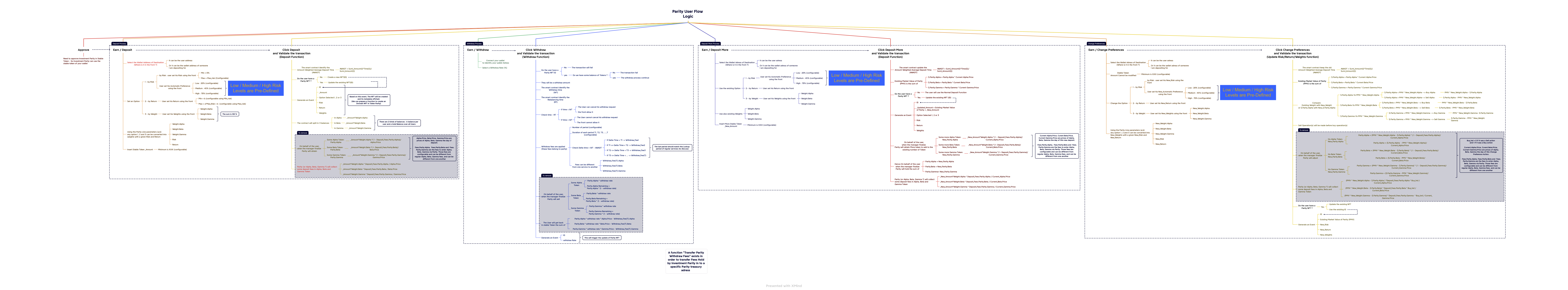
Figure 1: Parity Flow Flow Chart: Sequences of Steps for Periodic Fund Management

10 Appendix of Numerical Results

Each of the tables in this section are referenced in the main body of the article. Below, we provide supplementary descriptions for each table.

• Figure (2) shows three clouds of points representing the movement of Alpha, Beta and Gamma in Risk and Return space. Alpha is the right most, Beta is in the middle and Gamma is the left most set of points. The X-Axis is the risk axis and Y-axis is for returns.

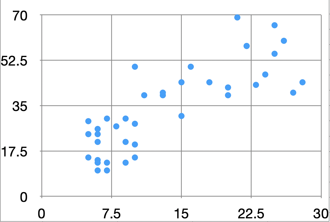
Figure 2: Parity Line: Alpha, Beta Gamma Combination Scatter Plot

• The Table in Figure (3) shows numerical examples related to combining Alpha, Beta and Gamma to get the Parity portfolio given their risk, return and correlation matrix. The weight of Alpha, $w_{\alpha}$is given by the formula,

  $$w_{\alpha}=\left(\frac{\frac{1}{\sigma_{\alpha t}}}{\frac{1}{\sigma_{\alpha t}}+\frac{1}{\sigma_{\beta t}}+\frac{1}{\sigma_{\gamma t}}}\right)$$ (186)

  Here, $\sigma_{\alpha t}$,$\sigma_{\beta t}$,$\sigma_{\gamma t}$ represent the volatilities of Alpha, Beta and Gamma at time $t$. A similar formula applies for Beta and Gamma.

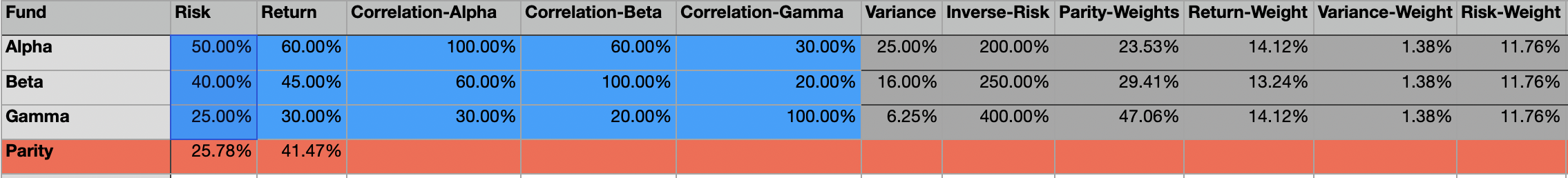
Figure 3: Parity Line: Alpha, Beta Gamma Combination Sample Data

• The Table in Figure (4) shows numerical examples using actual market data to combine Alpha, Beta and Gamma to get the Parity portfolio using the method in Section (5.2). Investors choose risk, return or directly the weights of Alpha and Beta. The numerical values presented below are from November 2022. The risk and return figures were estimated on a rolling 90 day basis. The security compositions of Alpha, Beta and Gamma are available upon request.

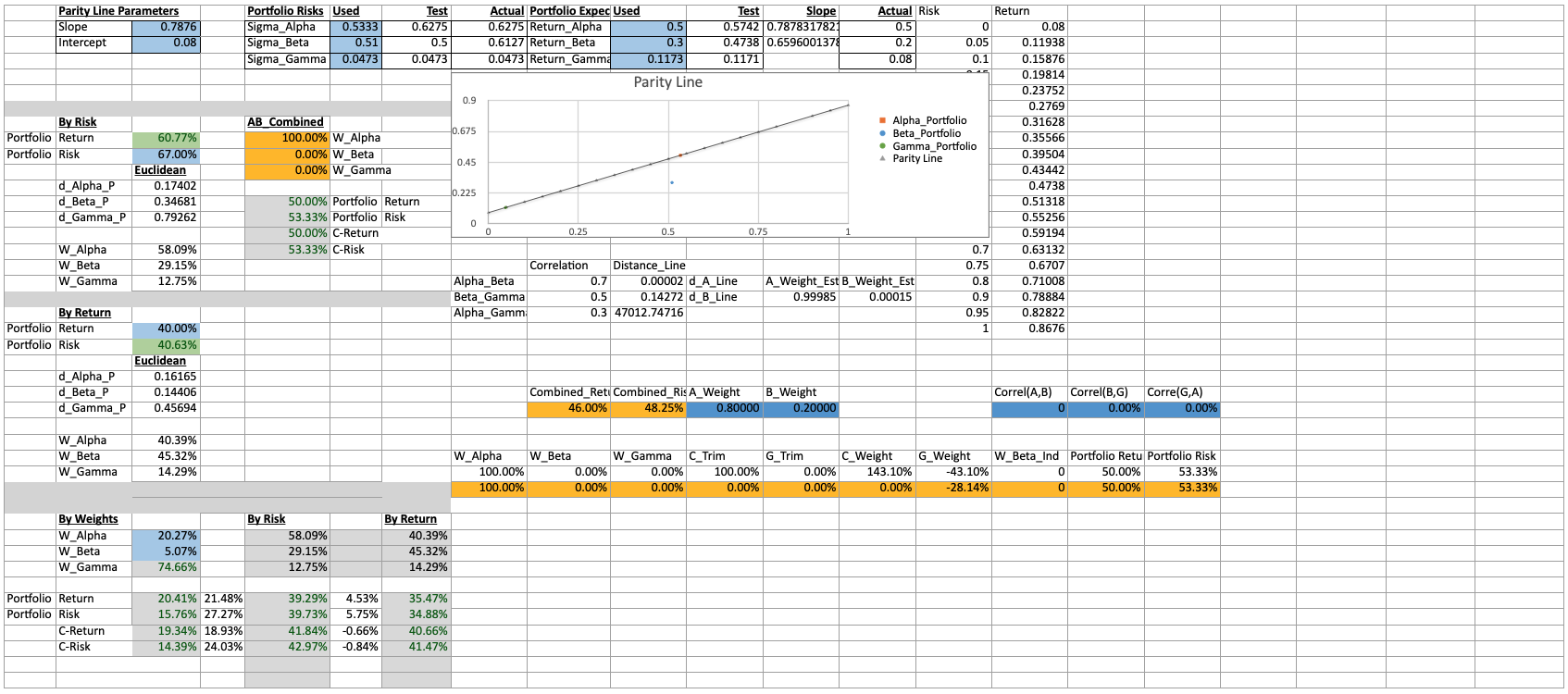
Figure 4: Parity Line: Alpha, Beta Gamma Combination Real Market Data

• The Table in Figure (5) shows numerical examples illustrating scenarios when investor return choices will vary and the portfolio risk and return are calculated based on the formulations in Section (5.2).

  • The columns in Figure (5) represent the following information respectively:

    1. Weight_Alpha corresponds to the calculated weight of Alpha.

    2. The other columns have similar nomenclatures and meaning.

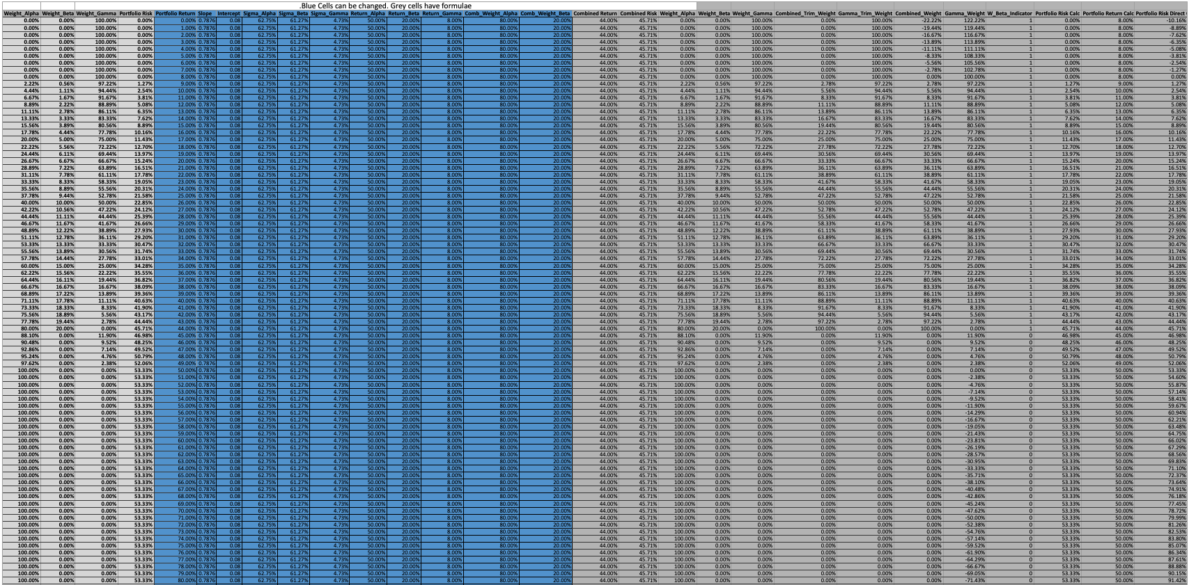
Figure 5: Parity Line: Return Scenario Analysis

• The Table in Figure (6) shows numerical examples illustrating scenarios when investor risk choices will vary and the portfolio risk and return are calculated based on the formulations in Section (5.2).

  • The columns in Figure (6) represent the following information respectively:

    1. Weight_Alpha corresponds to the calculated weight of Alpha.

    2. The other columns have similar nomenclatures and meaning.

Figure 6: Parity Line: Risk Scenario Analysis

• The Table in Figure (7) shows numerical examples illustrating scenarios when investor weight choices will vary and the portfolio return is incremented in steps of one percent The portfolio risk calculations are based on the formulations in Section (5.2).

  • The columns in Figure (7) represent the following information respectively:

    1. Weight_Alpha corresponds to the calculated weight of Alpha.

    2. The other columns have similar nomenclatures and meaning.

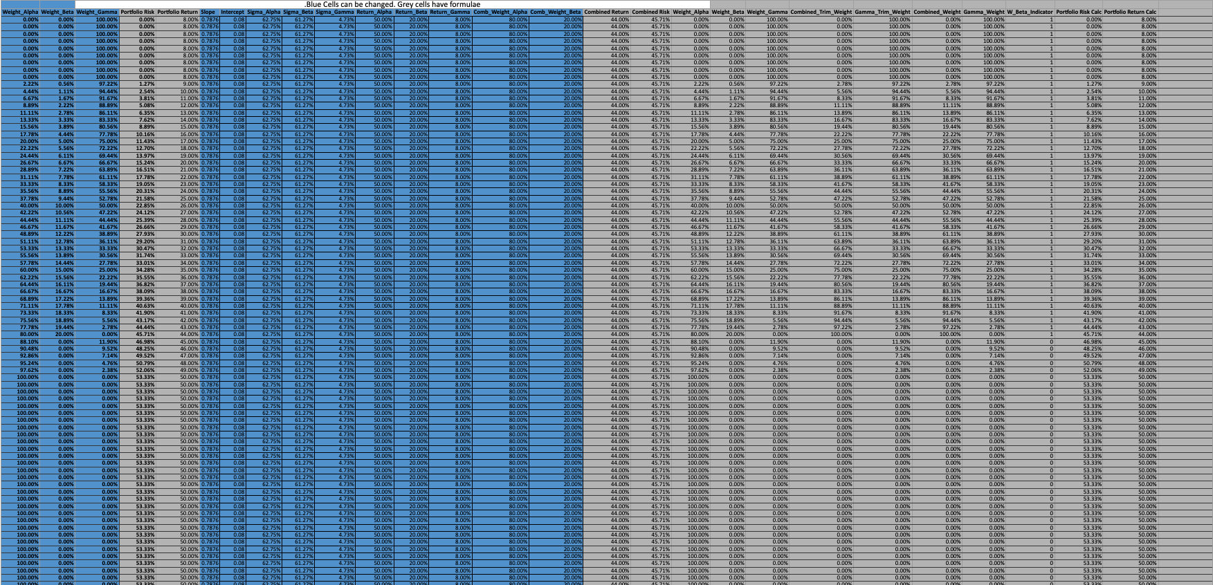
Figure 7: Parity Line: Weights and Return Scenario Analysis

• The Table in Figure (8) shows numerical examples illustrating scenarios when investor weight choices will vary and the portfolio risk is incremented in steps of one percent The portfolio return calculations are based on the formulations in Section (5.2).

  • The columns in Figure (8) represent the following information respectively:

    1. Weight_Alpha corresponds to the calculated weight of Alpha.

    2. The other columns have similar nomenclatures and meaning.

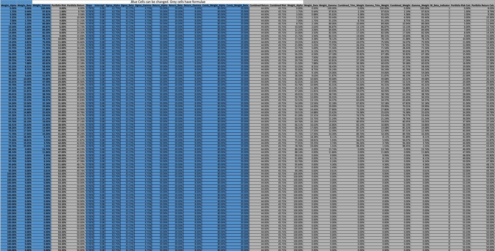
Figure 8: Parity Line: Weights and Risk Scenario Analysis

• The Table in Figure (9) shows numerical examples related to the method described in

  • The columns in Figure (9) represent the following information respectively:

    1. Time Step corresponds to the rebalancing event when the following actions happen by the corresponding investors and the state of their investment and the fund prices.

    2. The other columns have similar nomenclatures and meaning.

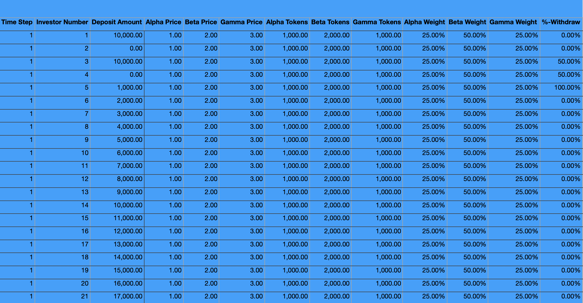
Figure 9: Parity Sequence of Steps: Investor Level Variables

• The Table in Figure (10) shows numerical examples related to the method described in

  • The columns in Figure (10) represent the following information respectively:

    1. $DepositPlusTokens corresponds to the dollar value of the deposit plus tokens for the corresponding investor.

    2. The other columns have similar nomenclatures and meaning.

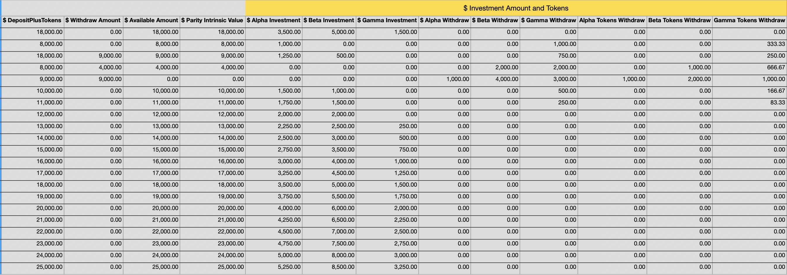
Figure 10: Parity Sequence of Steps: Investor Level Amounts and Tokens

• The Table in Figure (11) shows numerical examples related to the method described in

  • The columns in Figure (11) represent the following information respectively:

    1. $AIR is the raw value of the investment needed in Alpha that does not check if a corresponding withdraw is also happened for the investor in this row. Notice $AIR is positive and $AWR is negative in the first row. Hence only a net investment will happen into Alpha for this investor.

    2. $ATW is the raw value of the number of tokens that need to withdrawn from this investor’s allocation. In the first row the values are negative hence this investor only receives a net deposit of tokens - and no withdraws - based on his chosen risk and return preferences.

    3. The other columns have similar nomenclatures and meaning.

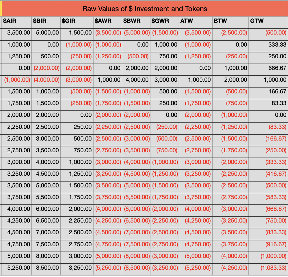
Figure 11: Parity Sequence of Steps: Investor Level Raw Values

• The Table in Figure (12) shows numerical examples related to the method described in Point (5g) in Algorithm (1) in Section (5.4.1). Notice that the Parity aggregate identity from Point (5g) in Algorithm (1) in Section (5.4.1) is satisfied.

  • The columns in Figure (12) represent the following information respectively:

    1. $Deposit corresponds to the total dollar value of the deposit received by the parity fund from all investors.

    2. The columns in Figure (12) have similar nomenclatures and meaning as the investor level illustrations in Figures (9; 10; 11).

Figure 12: Parity Sequence of Steps: Aggregate Deposits, Withdraws and Raw Values

• The Table in Figure (13) shows numerical examples related to the method described in Section (5.5).

  • The cell names and values in Figure (13) represent variables from Section (5.5).

    1. Slope (m) corresponds to the slope of the Parity Line as discussed in Section (5.5).

    2. The other cell names and values in Figure (13) have similar nomenclatures and meaning as the variables outlined in Section (5.5).

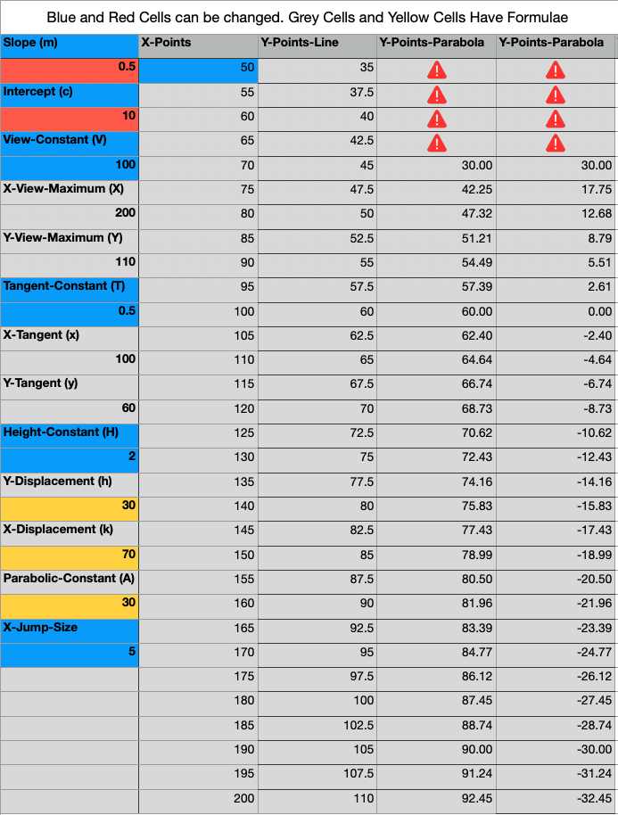
Figure 13: Parity Line and Parabolic Curve: X-Axis and Y-Axis Numerical Points

• The Illustrations in Figure (14) shows graphs related to the method described in Section (5.5) corresponding to the points given in Figure (13).

  • The X-Axis and Y-Axis in Figure (14) represent the risk and return values respectively.

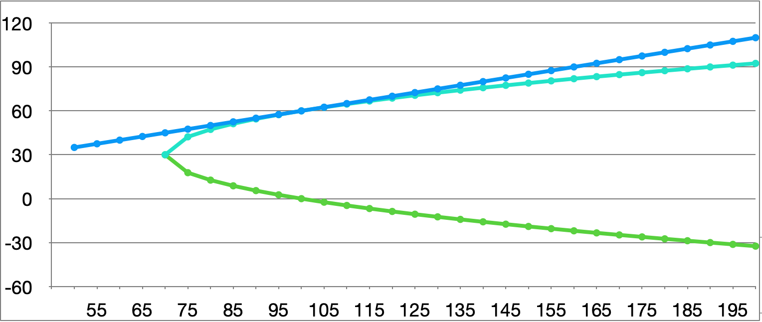
Figure 14: Parity Line and Parabolic Curve: Graphical Plots

11 Appendix of Explanations and End-notes

1. In modern portfolio theory, the efficient frontier (or portfolio frontier) is an investment portfolio which occupies the "efficient" parts of the risk–return spectrum. Formally, it is the set of portfolios which satisfy the condition that no other portfolio exists with a higher expected return but with the same standard deviation of return (i.e., the risk). Efficient Frontier, Wikipedia Link

2. Risk parity (or risk premia parity) is an approach to investment management which focuses on allocation of risk, usually defined as volatility, rather than allocation of capital. Risk Parity, Wikipedia Link

3. Star Trek is an American science fiction television series created by Gene Roddenberry that follows the adventures of the starship USS Enterprise (NCC-1701) and its crew. The show is set in the Milky Way galaxy, c. 2266–2269. The ship and crew are led by Captain James T. Kirk (William Shatner), First Officer and Science Officer Spock (Leonard Nimoy), and Chief Medical Officer Leonard H. "Bones" McCoy (DeForest Kelley). Shatner’s voice-over introduction during each episode’s opening credits stated the starship’s purpose:

   • Space: the final frontier. These are the voyages of the starship Enterprise. Its five-year mission: to explore strange new worlds, to seek out new life and new civilizations, to boldly go where no man has gone before. Star Trek: The Original Series, Wikipedia Link

4. Decentralized finance (often stylized as DeFi) offers financial instruments without relying on intermediaries such as brokerages, exchanges, or banks by using smart contracts on a blockchain. Decentralized Finance (DeFi), Wikipedia Link

5. The following are the four main types of blockchain decentralized financial products or services. We can also consider them as the main types of yield enhancement, or return generation, vehicles available in decentralized finance:

   1. Single-Sided Staking: This allows users to earn yield by providing liquidity for one type of asset, in contrast to liquidity provisioning on AMMs, which requires a pair of assets. Single Sided Staking, SuacerSwap Link

      1. Bancor is an example of a provider who supports single sided staking. Bancor natively supports Single-Sided Liquidity Provision of tokens in a liquidity pool. This is one of the main benefits to liquidity providers that distinguishes Bancor from other DeFi staking protocols. Typical AMM liquidity pools require a liquidity provider to provide two assets. Meaning, if you wish to deposit "TKN1" into a pool, you would be forced to sell 50% of that token and trade it for "TKN2". When providing liquidity, your deposit is composed of both TKN1 and TKN2 in the pool. Bancor Single-Side Staking changes this and enables liquidity providers to: Provide only the token they hold (TKN1 from the example above) Collect liquidity providers fees in TKN1. Single Sided Staking, Bancor Link

   2. AMM Liquidity Pairs (AMM LP): A constant-function market maker (CFMM) is a market maker with the property that that the amount of any asset held in its inventory is completely described by a well-defined function of the amounts of the other assets in its inventory (Hanson 2007). Constant Function Market Maker, Wikipedia Link

      This is the most common type of market maker liquidity pool. Other types of market makers are discussed in Mohan (2022). All of them can be grouped under the category Automated Market Makers. Hence the name AMM Liquidity Pairs. A more general discussion of AMMs, without being restricted only to the blockchain environment, is given in (Slamka, Skiera & Spann 2012).

   3. LP Token Staking: LP staking is a valuable way to incentivize token holders to provide liquidity. When a token holder provides liquidity as mentioned earlier in Point (5b) they receive LP tokens. LP staking allows the liquidity providers to stake their LP tokens and receive project tokens tokens as rewards. This mitigates the risk of impermanent loss and compensates for the loss. Liquidity Provider Staking, DeFactor Link

      1. Note that this is also a type of single sided staking discussed in Point (5a). The key point to remember is that the LP Tokens can be considered as receipts for the crypto assets deposits in an AMM LP Point (5b). These LP Token receipts can be further staked to generate additional yield.

   4. Lending: Crypto lending is the process of depositing cryptocurrency that is lent out to borrowers in return for regular interest payments. Payments are typically made in the form of the cryptocurrency that is deposited and can be compounded on a daily, weekly, or monthly basis. Crypto Lending, Investopedia Link; DeFi Lending, DeFiPrime Link; Top Lending Coins by Market Capitalization, Crypto.com Link.

      1. Crypto lending is very common on decentralized finance projects and also in centralized exchanges. Centralized cryptocurrency exchanges are online platforms used to buy and sell cryptocurrencies. They are the most common means that investors use to buy and sell cryptocurrency holdings. Centralized Cryptocurrency Exchanges, Investopedia Link

      2. Lending is a very active area of research both on blockchain and off chain (traditional finance) as well (Cai 2018; Zeng et al., 2019; Bartoletti, Chiang & Lafuente 2021; Gonzalez 2020; Hassija et al., 2020; Patel et al. , 2020).

      3. Lending is also a highly profitable business in the traditional financial world (Kashyap 2022-I). Investment funds, especially hedge funds, engage in borrowing securities to put on short positions depending on their investment strategies.Long only investment funds typically supply securities or lend their assets for a fee.

      4. In finance, a long position in a financial instrument means the holder of the position owns a positive amount of the instrument. Long Position in Finance, Wikipedia Link

      5. In finance, being short in an asset means investing in such a way that the investor will profit if the value of the asset falls. This is the opposite of a more conventional "long" position, where the investor will profit if the value of the asset rises. Short Position in Finance, Wikipedia Link

6. Modern portfolio theory (MPT), or mean-variance analysis, is a mathematical framework for assembling a portfolio of assets such that the expected return is maximized for a given level of risk. Modern Portfolio Theory, Wikipedia Link

7. The semivariance is defined as the expected squared deviation from the mean, calculated over those points that are no greater than the mean. Its square root is the semi-deviation. Downside Risk (Semi-Variance), Wikipedia Link

8. Fuzzy logic is a form of many-valued logic in which the truth value of variables may be any real number between 0 and 1. It is employed to handle the concept of partial truth, where the truth value may range between completely true and completely false. By contrast, in Boolean logic, the truth values of variables may only be the integer values 0 or 1. Fuzzy Logic, Wikipedia Link

9. Possibility theory is a mathematical theory for dealing with certain types of uncertainty and is an alternative to probability theory. It uses measures of possibility and necessity between 0 and 1, ranging from impossible to possible and unnecessary to necessary, respectively. Professor Lotfi Zadeh first introduced possibility theory in 1978 as an extension of his theory of fuzzy sets and fuzzy logic. Possibility Theory, Wikipedia Link

10. Probability theory or probability calculus is the branch of mathematics concerned with probability. The axioms of probability formalise it in terms of a probability space, which assigns a measure taking values between 0 and 1, termed the probability measure, to a set of outcomes called the sample space. Any specified subset of the sample space is called an event.Probability Theory, Wikipedia Link

11. Bayesian statistics is a theory in the field of statistics based on the Bayesian interpretation of probability where probability expresses a degree of belief in an event. The degree of belief may be based on prior knowledge about the event, such as the results of previous experiments, or on personal beliefs about the event. Bayesian Statistics, Wikipedia Link

    • Bayesian statistical methods use Bayes’ theorem to compute and update probabilities after obtaining new data. Bayes’ theorem describes the conditional probability of an event based on data as well as prior information or beliefs about the event or conditions related to the event.

12. Value at risk (VaR) is a measure of the risk of loss of investment/Capital. It estimates how much a set of investments might lose (with a given probability), given normal market conditions, in a set time period such as a day. Value at Risk (VaR), Wikipedia Link

13. Behavioral finance is the study of the influence of psychology on the behavior of investors or financial analysts. It assumes that investors are not always rational, have limits to their self-control and are influenced by their own biases.Behavioral Finance, Wikipedia Link

    1. Behavioral economics is the study of the psychological, cognitive, emotional, cultural and social factors involved in the decisions of individuals or institutions, and how these decisions deviate from those implied by classical economic theory. Behavioral Economics, Wikipedia Link

14. In finance, leverage (or gearing in the United Kingdom and Australia) is any technique involving borrowing funds to buy an investment, estimating that future profits will be more than the cost of borrowing. This technique is named after a lever in physics, which amplifies a small input force into a greater output force, because successful leverage amplifies the smaller amounts of money needed for borrowing into large amounts of profit. Leverage (Finance), Wikipedia Link

15. In finance, risk factors are the building blocks of investing, that help explain the systematic returns in equity market, and the possibility of losing money in investments or business adventures. Risk Factor (Finance), Wikipedia Link

16. In financial economics, asset pricing refers to a formal treatment and development of two interrelated pricing principles - either general equilibrium asset pricing or rational asset pricing. Asset Pricing, Wikipedia Link

17. Convex optimization is a subfield of mathematical optimization that studies the problem of minimizing convex functions over convex sets (or, equivalently, maximizing concave functions over convex sets). Convex Optimization, Wikipedia Link

18. The P versus NP problem is a major unsolved problem in theoretical computer science. In informal terms, it asks whether every problem whose solution can be quickly verified can also be quickly solved. P versus NP problem, Wikipedia Link

19. In computational complexity theory, NP-hardness (non-deterministic polynomial-time hardness) is the defining property of a class of problems that are informally "at least as hard as the hardest problems in NP". NP Hardness, Wikipedia Link

20. In computational complexity theory, NP (nondeterministic polynomial time) is a complexity class used to classify decision problems. NP is the set of decision problems for which the problem instances, where the answer is "yes", have proofs verifiable in polynomial time by a deterministic Turing machine, or alternatively the set of problems that can be solved in polynomial time by a nondeterministic Turing machine. NP (Complexity), Wikipedia Link

21. Principal component analysis (PCA) is a popular technique for analyzing large datasets containing a high number of dimensions/features per observation, increasing the interpretability of data while preserving the maximum amount of information, and enabling the visualization of multidimensional data. Formally, PCA is a statistical technique for reducing the dimensionality of a dataset. Principal Component Analysis, Wikipedia Link

22. A graphical user interface, or GUI, is a form of user interface that allows users to interact with electronic devices through graphical icons and visual indicators such as secondary notation. Graphical User Interface, Wikipedia Link

23. A smart contract is a computer program or a transaction protocol that is intended to automatically execute, control or document events and actions according to the terms of a contract or an agreement. The objectives of smart contracts are the reduction of need for trusted intermediators, arbitration costs, and fraud losses, as well as the reduction of malicious and accidental exceptions. Smart contracts are commonly associated with cryptocurrencies, and the smart contracts introduced by Ethereum are generally considered a fundamental building block for decentralized finance (DeFi) and NFT applications. Smart Contract, Wikipedia Link

24. A non-fungible token (NFT) is a unique digital identifier that is recorded on a blockchain, and is used to certify ownership and authenticity. It cannot be copied, substituted, or subdivided. The ownership of an NFT is recorded in the blockchain and can be transferred by the owner, allowing NFTs to be sold and traded. Non-Fungible Token (NFT), Wikipedia Link

25. In mathematics, a metric space is a set together with a notion of distance between its elements, usually called points. The distance is measured by a function called a metric or distance function. Metric Space, Wikipedia Link

26. A Stablecoin is a type of cryptocurrency where the value of the digital asset is supposed to be pegged to a reference asset, which is either fiat money, exchange-traded commodities (such as precious metals or industrial metals), or another cryptocurrency. Stable Coin, Wikipedia Link

27. Net Asset Value is the net value of an investment fund’s assets less its liabilities, divided by the number of shares outstanding. NAV, Investopedia Link

28. In mathematics, a parabola is a plane curve which is mirror-symmetrical and is approximately U-shaped. It fits several superficially different mathematical descriptions, which can all be proved to define exactly the same curves. Parabola, Wikipedia Link

    1. One description of a parabola involves a point (the focus) and a line (the directrix). The focus does not lie on the directrix. The parabola is the locus of points in that plane that are equidistant from the directrix and the focus.

29. In finance, the Sharpe ratio (also known as the Sharpe index, the Sharpe measure, and the reward-to-variability ratio) is a way to examine the performance of an investment by adjusting for its risk. The ratio measures the excess return (or risk premium) per unit of deviation in an investment asset or a trading strategy, typically referred to as risk, named after William F. Sharpe. Sharpe Ratio, Wikipedia Link

30. In probability theory and statistics, skewness is a measure of the asymmetry of the probability distribution of a real-valued random variable about its mean. The skewness value can be positive, zero, negative, or undefined. Skewness, Wikipedia Link

31. In probability theory and statistics, kurtosis (from Greek: kyrtos or kurtos, meaning "curved, arching") is a measure of the "tailedness" of the probability distribution of a real-valued random variable. Like skewness, kurtosis describes a particular aspect of a probability distribution. There are different ways to quantify kurtosis for a theoretical distribution, and there are corresponding ways of estimating it using a sample from a population. Kurtosis, Wikipedia Link

32. Gas is a unit of account within the EVM used in the calculation of the transaction fee, which is the amount of ETH a transaction’s sender must pay to the network to have the transaction included in the blockchain. Ethereum (Gas Fees) Wikipedia Link

33. A decentralized autonomous organization (DAO), sometimes called a decentralized autonomous corporation (DAC), is an organization managed in whole or in part by decentralized computer program, with voting and finances handled through a blockchain. In general terms, DAOs are member-owned communities without centralized leadership. The precise legal status of this type of business organization is unclear. Decentralized Autonomous Organization (DAO), Wikipedia Link

34. Ethereum, which was conceived in 2013 and launched in 2015 (Wood 2014; Tapscott & Tapscott 2016; Dannen 2017), provided a remarkable innovation in terms of making blockchain based systems Turing complete (or theoretically being able to do what any computer can do: Sipser 2006).

    1. Ethereum is a decentralized, open-source blockchain with smart contract functionality. Ether (Abbreviation: ETH) is the native cryptocurrency of the platform. Among cryptocurrencies, ether is second only to bitcoin in market capitalization. Ethereum, Wikipedia Link

    2. In computability theory, a system of data-manipulation rules (such as a computer’s instruction set, a programming language, or a cellular automaton) is said to be Turing-complete or computationally universal if it can be used to simulate any Turing machine. Turing Completeness, Wikipedia Link

       A Turing machine is a mathematical model of computation describing an abstract machine that manipulates symbols on a strip of tape according to a table of rules. Despite the model’s simplicity, it is capable of implementing any computer algorithm. Turing Machine, Wikipedia Link

35. Open-end mutual funds are purchased from or sold to the issuer at the net asset value of each share as of the close of the trading day in which the order was placed, as long as the order was placed within a specified period before the close of trading. They can be traded directly with the issuer. Mutual Fund, Wikipedia Link

36. Mutual Funds typically pay their regular and recurring, fund-wide operating expenses out of fund assets, rather than by imposing separate fees and charges directly on investors. Mutual Fund Fees, Wikipedia Link

37. A hedge fund is a pooled investment fund that trades in relatively liquid assets and is able to make extensive use of more complex trading, portfolio-construction, and risk management techniques in an attempt to improve performance, such as short selling, leverage, and derivatives. Hedge Fund, Wikipedia Link

38. An exchange-traded fund (ETF) is a type of investment fund and exchange-traded product, i.e. they are traded on stock exchanges. ETFs are similar in many ways to mutual funds, except that ETFs are bought and sold from other owners throughout the day on stock exchanges whereas mutual funds are bought and sold from the issuer based on their price at day’s end. Exchange Traded Fund, Wikipedia Link

12 Appendix of Proofs of Propositions

12.1 Parity Line Expected Return

Proof.

Proof of Proposition (1) is given here. Using the weights - indicated in the statement of the proposition - for Alpha, Beta and Gamma we get the expected return chosen by the investor as below,

$$\left[w_{\alpha}E\left(R_{\alpha}\right)\right]+\left[w_{\beta}E\left(R_{\beta}\right)\right]+\left[w_{\gamma}E\left(R_{\gamma}\right)\right]=\left[\left(w_{c}\right)\left(w_{c\alpha}\right)E\left(R_{\alpha}\right)\right]+\left[\left(w_{c}\right)\left(w_{c\beta}\right)E\left(R_{\beta}\right)\right]+\left[\left(w_{\gamma}\right)E\left(R_{\gamma}\right)\right]$$ (187)

$$=\left[\left(\frac{\left[E\left(R_{i}\right)-E\left(R_{\gamma}\right)\right]}{\left[E\left(R_{c}\right)-E\left(R_{\gamma}\right)\right]}\right)\left(w_{c\alpha}\right)E\left(R_{\alpha}\right)\right]$$ (188)

$$+\left[\left(\frac{\left[E\left(R_{i}\right)-E\left(R_{\gamma}\right)\right]}{\left[E\left(R_{c}\right)-E\left(R_{\gamma}\right)\right]}\right)\left(w_{c\beta}\right)E\left(R_{\beta}\right)\right]$$ (189)

$$+\left[\left(\frac{\left[E\left(R_{i}\right)-E\left(R_{c}\right)\right]}{\left[E\left(R_{\gamma}\right)-E\left(R_{c}\right)\right]}\right)E\left(R_{\gamma}\right)\right]$$ (190)

$$=\left[\left(\frac{\left[E\left(R_{i}\right)\left(w_{c\alpha}\right)E\left(R_{\alpha}\right)-E\left(R_{\gamma}\right)\left(w_{c\alpha}\right)E\left(R_{\alpha}\right)\right]}{\left[E\left(R_{c}\right)-E\left(R_{\gamma}\right)\right]}\right)\right]$$ (191)

$$+\left[\left(\frac{\left[E\left(R_{i}\right)\left(w_{c\beta}\right)E\left(R_{\beta}\right)-E\left(R_{\gamma}\right)\left(w_{c\beta}\right)E\left(R_{\beta}\right)\right]}{\left[E\left(R_{c}\right)-E\left(R_{\gamma}\right)\right]}\right)\right]$$ (192)

$$-\left[\left(\frac{\left[E\left(R_{i}\right)-\left[w_{c\alpha}E\left(R_{\alpha}\right)\right]-\left[w_{c\beta}E\left(R_{\beta}\right)\right]\right]}{\left[E\left(R_{c}\right)-E\left(R_{\gamma}\right)\right]}\right)E\left(R_{\gamma}\right)\right]$$ (193)

$$=\left[\left(\frac{\left[E\left(R_{i}\right)\left(w_{c\alpha}\right)E\left(R_{\alpha}\right)-E\left(R_{\gamma}\right)\left(w_{c\alpha}\right)E\left(R_{\alpha}\right)\right]}{\left[E\left(R_{c}\right)-E\left(R_{\gamma}\right)\right]}\right)\right]$$ (194)

$$+\left[\left(\frac{\left[E\left(R_{i}\right)\left(w_{c\beta}\right)E\left(R_{\beta}\right)-E\left(R_{\gamma}\right)\left(w_{c\beta}\right)E\left(R_{\beta}\right)\right]}{\left[E\left(R_{c}\right)-E\left(R_{\gamma}\right)\right]}\right)\right]$$ (195)

$$-\left[\left(\frac{\left[E\left(R_{i}\right)E\left(R_{\gamma}\right)-\left[E\left(R_{\gamma}\right)w_{c\alpha}E\left(R_{\alpha}\right)\right]-\left[E\left(R_{\gamma}\right)w_{c\beta}E\left(R_{\beta}\right)\right]\right]}{\left[E\left(R_{c}\right)-E\left(R_{\gamma}\right)\right]}\right)\right]$$ (196)

$$=\left[\left(\frac{\left[E\left(R_{i}\right)\left(w_{c\alpha}\right)E\left(R_{\alpha}\right)\right]}{\left[E\left(R_{c}\right)-E\left(R_{\gamma}\right)\right]}\right)\right]$$ (197)

$$+\left[\left(\frac{\left[E\left(R_{i}\right)\left(w_{c\beta}\right)E\left(R_{\beta}\right)\right]}{\left[E\left(R_{c}\right)-E\left(R_{\gamma}\right)\right]}\right)\right]$$ (198)

$$-\left[\left(\frac{\left[E\left(R_{i}\right)E\left(R_{\gamma}\right)\right]}{\left[E\left(R_{c}\right)-E\left(R_{\gamma}\right)\right]}\right)\right]$$ (199)

$$=\left[E\left(R_{i}\right)\left(\frac{\left[\left(w_{c\alpha}\right)E\left(R_{\alpha}\right)+\left(w_{c\beta}\right)E\left(R_{\beta}\right)-E\left(R_{\gamma}\right)\right]}{\left[E\left(R_{c}\right)-E\left(R_{\gamma}\right)\right]}\right)\right]$$ (200)

$$=\left[E\left(R_{i}\right)\left(\frac{\left[E\left(R_{c}\right)-E\left(R_{\gamma}\right)\right]}{\left[E\left(R_{c}\right)-E\left(R_{\gamma}\right)\right]}\right)\right]$$ (201)

$$=E\left(R_{i}\right)$$ (202)

∎

13 Return and Risk (Volatility) Calculations

The weight calculation depends on calculating the return of asset prices on a daily basis (could be at other frequencies as well, but we start with daily returns). The return will be the continuously compounded measure. The volatility will be the standard deviation of the continuously compounded returns over a historical time period, generally around 90 days. The volatility will need to be calculated on a rolling 90 days basis.

1. Continuously Compounded Return, $R_{t}$, at any time $t$ is given by the logarithm of the ratio of the Price at time $t$, $P_{t}$, and the Price at time $t-1$, $P_{t-1}$, as shown below,

   $$R_{t}=\ln\left(\frac{P_{t}}{P_{t-1}}\right)$$ (203)

2. Volatility at time $t$, $\sigma_{t}$ is calculated as below using the average return, $\bar{R}_{t}$, at time $t$ and then calculating the standard deviation. It can be done directly if suitable libraries are available. $\sigma_{t}^{2}$ is the variance at time $t$. Here, $T=90$ unless otherwise stated.

   $$\bar{R}_{t}=\left(\frac{1}{T}\right)\sum_{i=t}^{t-T}R_{i}$$ (204)

   $$\sigma_{t}^{2}=\left(\frac{1}{T-1}\right)\sum_{i=t}^{t-T}\left(R_{i}-\bar{R}_{t}\right)^{2}$$ (205)

   $$\sigma_{t}=\sqrt{\left(\frac{1}{T-1}\right)\sum_{i=t}^{t-T}\left(R_{i}-\bar{R}_{t}\right)^{2}}$$ (206)

3. Calculate the volatility for the longest historical time period possible for each asset. Possibly for the last 360 days or longer. Some new assets might have a relatively shorter price time series, and it is okay to calculate volatility for those assets for the number of days for which prices are available.

14 Appendix of Additional Illustrations

Figure 16: Classification of Environmental Risks