DFS-based fast crack detection

Abstract

In this paper, we propose an fast method for crack detection in 3D computed tomography (CT) images. Our approach combines the Maximal Hessian Entry filter and a Deep-First Search algorithm-based technique to strike a balance between computational complexity and accuracy. Experimental results demonstrate the effectiveness of our approach in detecting the crack structure with predefined misclassification probability.

Keywords: Deep-First Search algorithm, Hessian-based filter, crack detection, classification.

MSC2020: Primary: 68U10; Secondary: 68R10, 94A08.

1 Introduction

Concrete is the traditional material of choice for constructing buildings, bridges, and road infrastructure, underscoring the critical importance of safety in their design, monitoring, and maintenance. In the pursuit of enhancing safety, numerous studies have been conducted to understand the structure of concrete [6], testing it under some specific types of loadings.

A modern visualizing technique is high resolution CT gray scale imaging, which shows cracks as a collection of connected voxels carrying low gray values. Due to the nature of cracks, which typically form a flat surface within the material, the crack segmentation can be done by applying several classical methods [12, 5, 3], or implementing some Machine Leaning algorithms [14, 2, 13]. They usually perform well, classifying crack voxels as anomaly with high performance [1]. However, in real-world scenarios, the complexity of concrete including cracks, air pores, stones, or steel fibers often necessitates the enhancement of classical segmentation techniques, leading to increased computational demands. Furthermore, the shortage of training data due to high costs of stress tests and CT imaging complicates the training of machine learning models. One approach to address this challenge involves creating a large collection of semi-synthetic 3D CT images [8, 9] which simulates real material and crack behavior based on minimum-weight surfaces in bounded Voronoi diagrams. However, for extremely large input 3D images that modern CT scanning are able to produce (e.g. of size $10000^{2}\times 2000$), runtimes of crack detection algorithms become a major concern.

Therefore, in order to overcome this problem, a statistical approach can be employed to pre-identify anomaly regions, reducing unnecessary computations. An effective strategy may involve applying a relatively simple crack segmentation method, followed by the examination of subregion geometry. The Deep-First Search algorithm (DFS) is identified as a promising solution for this task. Originating from the work of French mathematician C. Trémaux, DFS has been widely adopted in graph theory [7, 15] and connectivity problems [4], enabling the detection of connected components or object labeling within binary images. By focusing on surface examination within smaller images and using natural crack elongation, DFS can effectively identify crack regions within a reasonable timeframe. Moreover, the framework [10] proposed for crack detection in real 3D CT images requires the computations of geometric properties for each subregion belonging to the partition of the original input image. In this context, DFS reduces the amount of computations by excluding crack-free image regions.

This paper presents a two-phase procedure involving crack segmentation and a DFS-based algorithm for crack detection. Section 2 outlines a simple yet effective filter designed in [10] to generate a binary image with high sensitivity, preserving crack structure while accommodating a certain level of noise. Subsequently, Section 3 provides insights into the implementation of the DFS algorithm to swiftly detect cracks in smaller regions. Additionally, Section 4 shows the numerical experiments with methods from Section 2 and 3 employed for both semi-synthetic and real CT images, provided by Technical University of Kaiserslautern and Fraunhofer ITWM. Finally, Section 5 offers a summary of the key findings and identifies potential challenges for future research. The whole procedure is describe in Diagram 1.

Figure 1: 6-step process diagram for crack localization in 3D concrete images

2 Crack segmentation

In order to use the DFS algorithm for crack detection in a 3D gray scale image, one first needs to apply certain fast image segmentation methods. In this paper, we utilize a Hessian-based filter called Maximal Hessian Entry filter [10]. Let $I=\{I(p)\in[0,1],p\in W\subset\mathbb{Z}^{3}\}$ be an input 3D gray scale image. For a prespecified value of $\sigma>0$, let $G$ be the 3-dimensional Gaussian kernel, $G(p;\sigma)=(2\pi\sigma^{2})^{-3/2}\exp\{-\left\|p\right\|_{2}^{2}/(2\sigma^{2})\}$ with scale parameter $\sigma>0$, where $\|\cdot\|_{2}$ is the Euclidean norm in $\mathbb{R}^{3}$. The Hessian matrix $H(p;\sigma)$ of the image $I$ at a voxel $p=(p_{1},p_{2},p_{3})\in W$ is given by

$$H(p;\sigma)=\left(H_{i,j}(p;\sigma)\right)_{i,j=1}^{3},$$

where

$$H_{i,j}(p;\sigma):=\sigma I(p)*\frac{\partial^{2}}{\partial p_{i}\partial p_{j}}G(p;\sigma),\ i,j=1,2,3\text{ and}*\text{denotes the usual convolution operation.}$$

Let

$$L_{\sigma}(I)=\left\{L_{\sigma}(I,p)=\max_{i,j=1,2,3}\left(H_{i,j}(p;\sigma),0\right),\ p\in W\right\}.$$

Denote by $\mu(L_{\sigma}(I))$ and $sd(L_{\sigma}(I))$ the sample mean and the sample standard deviation of all gray values within $L_{\sigma}(I)$. For a threshold $T_{\sigma}(I)=\mu(L_{\sigma}(I))+3sd(L_{\sigma}(I))$, one can obtain a binarized image $L_{\sigma}^{*}(I)$ as follows:

$$L_{\sigma}^{*}(I)=\{L_{\sigma}^{*}(I,p)=\mathds{1}\{L_{\sigma}(I,p)\geq T_{\sigma}(I)\},\ p\in W\}.$$

Let $\mathcal{S}$ be a finite range of values of the smoothing parameter $\sigma$. The final outcome of the Maximal Hessian Entry filter applied to image $I$ is computed by

$$L_{\mathcal{S}}(I)=\{L_{\mathcal{S}}(I,p)=\max_{\sigma\in S}L_{\sigma}^{*}(I,p),\ p\in W\}.$$

The performance comparison between this and other classical crack segmentation methods has been investigated in [1] and [10]. It is worth noting that the structure of cracks in the input image $I$ is well preserved in the filtered image $L_{\mathcal{S}}(I)$ with a certain level of noise, for both semi-synthetic images $I_{1},I_{2},I_{3}$ and real CT images $I_{4},I_{5}$ provided by Technical University of Kaiserslautern and Fraunhofer ITWM, see Figure 2. It allows the geometric detection of local structures in concrete (such as air pores, steel fibres and cracks) by means of the following DFS algorithm.

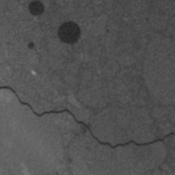
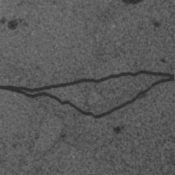
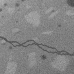
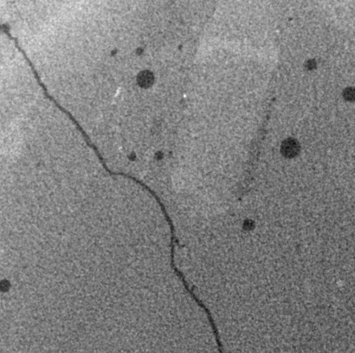
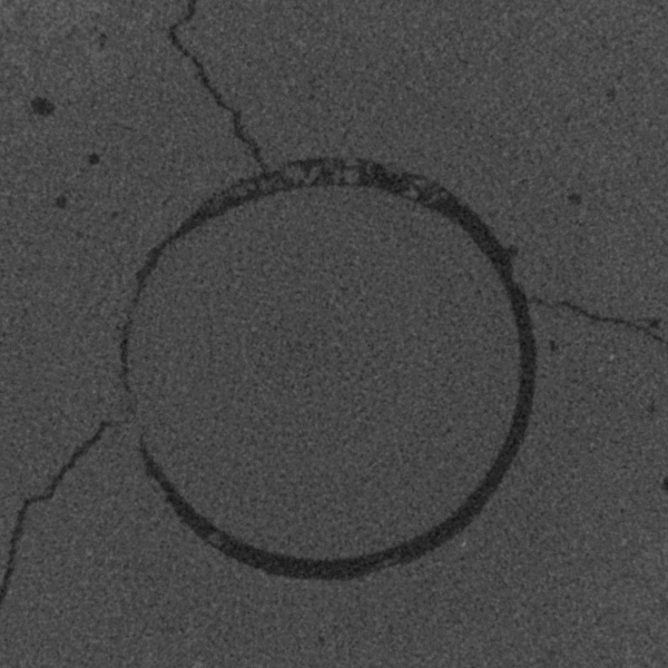
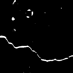
(a) $I_{1}$

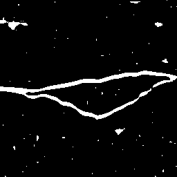
(b) $I_{2}$

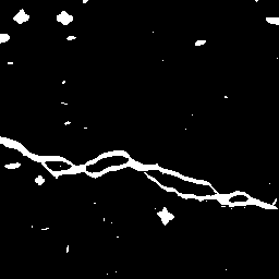
(c) $I_{3}$

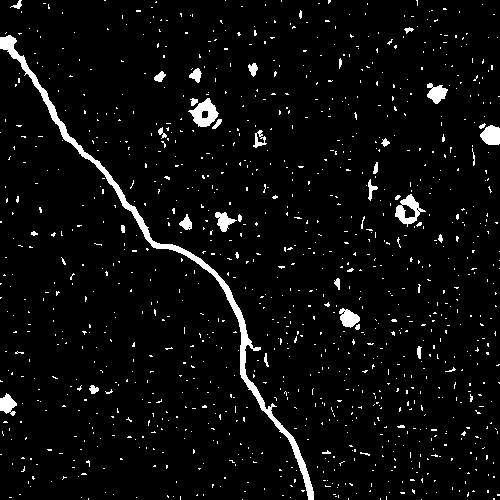
(d) $I_{4}$

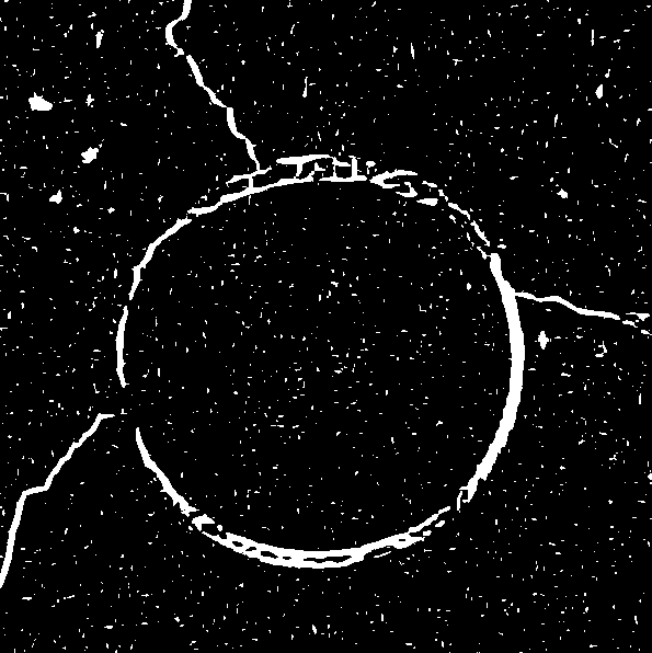
(e) $I_{5}$

Figure 2: First row: Slices of input gray scale images $I_{j},j=1,\ldots,5$. Second row: Corresponding slices of binary images $L_{\mathcal{S}}(I_{j}),j=1,\ldots,5$ computed using the Maximal Hessian Entry filter.

3 DFS-based algorithm in crack detection

In this section, we present a method employing the DFS algorithm to identify crack-containing regions within 3D binary images. Given the elongated flat 2D structure of cracks, it becomes evident that if cracks exist within a sufficiently small cubic subregion $\widetilde{W}$, they are likely to intersect its boundary $\partial\widetilde{W}$, see Figure 3. Hence, determining whether a small region $\widetilde{W}$ contains a crack depends on our ability to detect cracks on one of the facets. Therefore, our detection procedure will be applied to 2D surface $\widetilde{W}$ instead of 3D volume $W$, which significantly reduces the computational cost.

The DFS algorithm is commonly employed for detecting connected components or labeling objects within 2D binary images. Its implementation requires the construction of a graph $G=(V,E)$ over the image domain, where $V$ represents the set of pixels, and $E$ is the set of the edges between vertices in $V$ with respect to 4-connectivity neighborhood relation. Since the complexity of DFS algorithm is $O(\#V+\#E)$. Here and in what follows, $\#A$ is the cardinality of a finite set $A$, performing DFS consequently over a sufficiently large collection of 2D images is challenging in terms of run time, which is one of our primary concerns.

To address this limitation, a novel approach involves constructing a modified image graph with a reduced number of vertices, leveraging prior knowledge from the binary image, particularly the identification of pixels representing cracks. Consider a binary image $J=\{J(p)\in\{0,1\},p\in\mathcal{W}\},\ \mathcal{W}=[0,a]\times[0,b]\cap\mathbb{Z}^{2}$. For any mesh size $\Delta\in\mathbb{N}$, the following procedure is proposed to obtain such a graph:

1. Define the lattice graph $G_{\Delta}=(V_{\Delta},E_{\Delta})$, where $V_{\Delta}=\mathcal{W}\cap\Delta\mathbb{Z}^{2}$ represents the set of vertices and $E_{\Delta}=\{(e_{1},e_{2})\mid e_{1},e_{2}\in V_{\Delta},\|e_{1}-e_{2}\|_{2}=\Delta\}$ denotes the collection of edges, with $\|\cdot\|_{2}$ being the Euclidean norm in $\mathbb{R}^{2}$.

2. Identify the set $H=\{p\in V_{\Delta}\mid J(p)=1\}$, representing foreground pixels within $J$ and belonging to $V_{\Delta}$.

3. Define the set $K=\{p_{1}\in V_{\Delta}\setminus H\mid\|p_{1}-p\|_{\infty}=1,p\in H\}$, finding all neighbors of $H$ in the graph, where $\|\cdot\|_{\infty}$ denotes the maximum norm in $\mathbb{R}^{2}$.

4. Remove all edges from $E$ that do not have vertices in $K$, resulting in $E_{K}=\{(e_{1},e_{2})\in E\mid e_{1},e_{2}\in K\}$.

5. Define the new graph $G^{*}=(K,E_{K})$.

In context of crack detection we put $J=\{L_{\mathcal{S}}(I,p):p\in\mathcal{W}\}$ where $\mathcal{W}$ is a facet of $\partial\widetilde{W}\cap\mathbb{Z}^{2}$. Foreground pixels correspond to a crack phase.

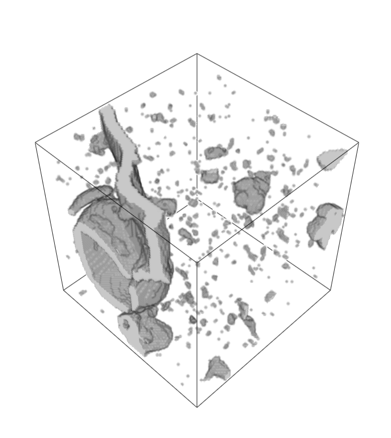
(a) $100^{3}$ region

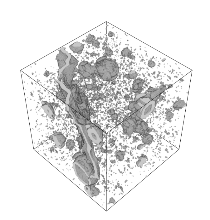
(b) $200^{3}$ region

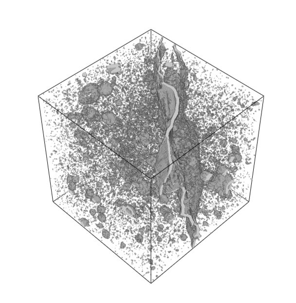
(c) $300^{3}$ region

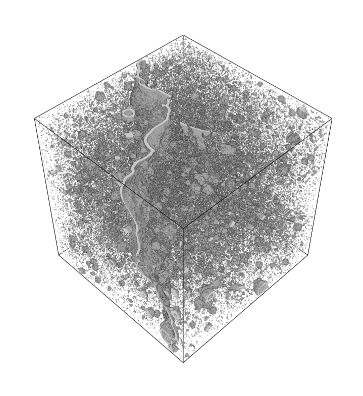
(d) $L_{\mathcal{S}}(I_{4})$

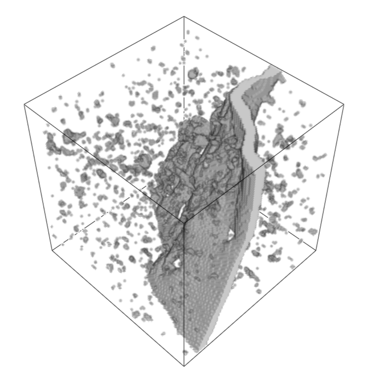
(e) $100^{3}$ region

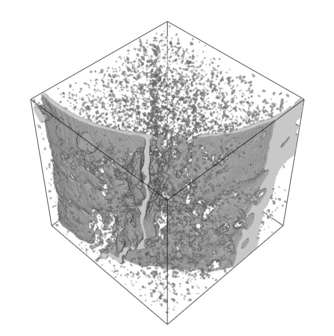
(f) $200^{3}$ region

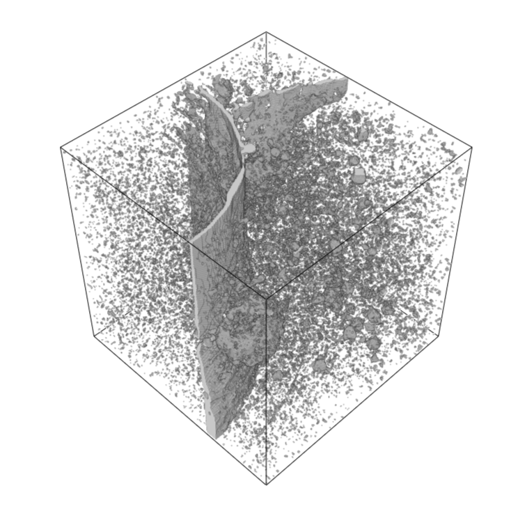
(g) $300^{3}$ region

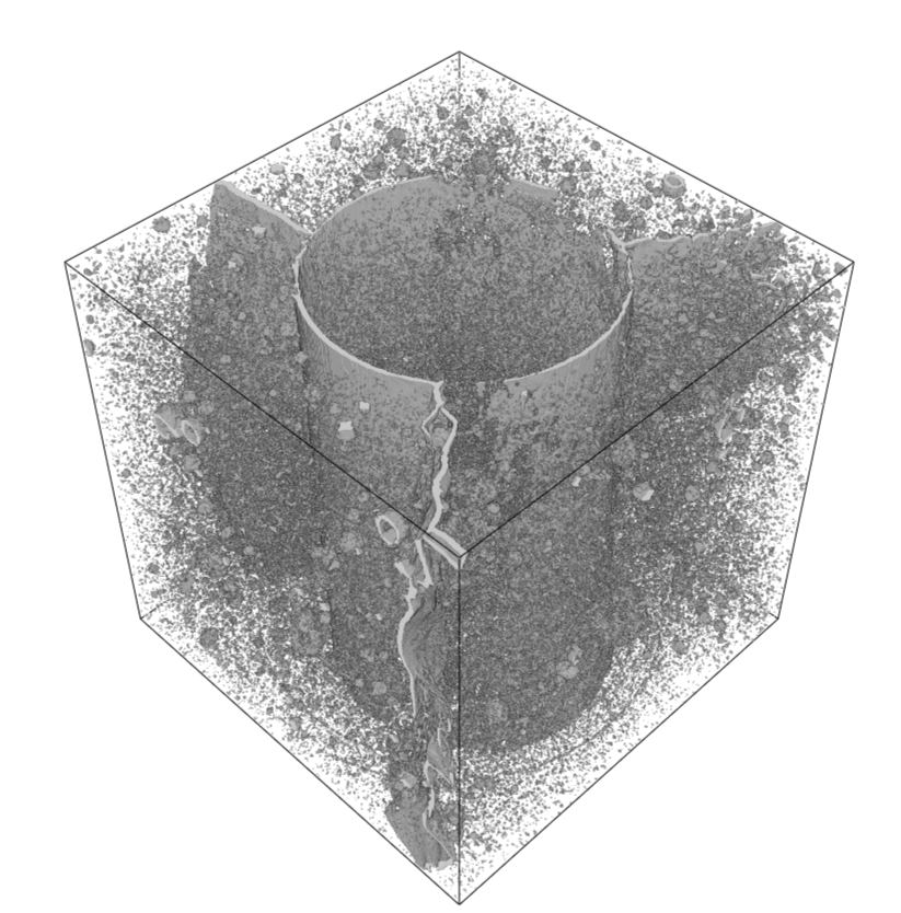
(h) $L_{\mathcal{S}}(I_{5})$

Figure 3: 3D visualization of subregions $\widetilde{W}$ of different size of binary images $L_{\mathcal{S}}(I_{4})$ and $L_{\mathcal{S}}(I_{5})$.

As illustrated in Figure 4, appropriate settings for $\Delta$ in the above procedure result in a less complex graph $G^{*}$ with lower cardinalities of both sets of vertices $K$ and edges $E_{K}$. Consequently, any computation performed over such a simplified graph offers advantages in terms of computational cost. Moreover, in the presence of cracks on one of the surfaces, the graph is capable of localizing them, as shown in (b), (c).

However, when $\Delta$ is large compared to the crack width, denoted by $w$, it is likely that our procedure is unable to find the set $H$, as now $\#V_{\Delta}$ will be small. This prevents any attempt to capture the pixels belonging to cracks, resulting in a graph with numerous small connected components that bound the pixels belonging to air pores, see Figure 4, (e), (f). Therefore, it is necessary to control the probability of missing anomaly pixels using this grid lattice. For simplicity, one can consider a crack as a convex body $C$. Let $C_{0}$ be an intersection of $C$ with a facet of a small region $\widetilde{W}=[a,b]^{3},\ a<b$. One needs to give an upper bound for the probability $\mathbb{P}\{C_{0}\cap\Delta\mathbb{Z}^{d}=\emptyset\}$.

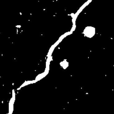
(a) The $200^{2}$ binary image $L_{\mathcal{S}}^{1}$

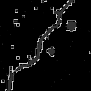
(b) The graph $G^{*}_{1}$
with $\Delta=3$

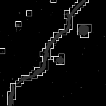
(c) The graph $G^{*}_{1}$
with $\Delta=5$

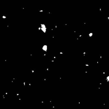
(d) The $200^{2}$ binary image $L_{\mathcal{S}}^{2}$

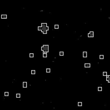
(e) The graph $G^{*}_{2}$
with $\Delta=3$

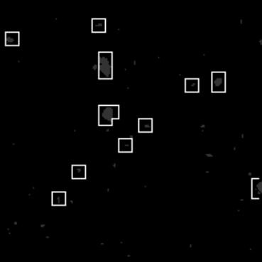
(f) The graph $G^{*}_{2}$
with $\Delta=5$

Figure 4: 2D binary images $J$ with obtained graph $G^{*}$ by our procedure.

To this end, we use the following

Theorem 1.

([11, Theorem 4]) For every $\epsilon>0$, there exist constants $\bar{c}$ and $\bar{w}$ such that if $C_{0}$ is a planar convex body with area $|C_{0}|>\bar{c}$ and mean width $w_{0}<\bar{w}$, then

$$\mathbb{P}\{\rho(C_{0})\cap\Delta\mathbb{Z}^{2}=\emptyset\}<\frac{\Delta^{2}}{4}\cdot\frac{1+\epsilon}{|C_{0}|},$$

where $\rho(C_{0})$ is congruent to $C_{0}$ under a random isometry $\rho$ of $\mathbb{R}^{2}$.

This suggests that, if one seeks to control the probability of missing a crack $C_{0}$ at level $\alpha$, then the maximum mesh size $\Delta_{\max}(\alpha)$ can be chosen from inequality $\frac{\Delta^{2}}{4}\cdot\frac{1+\epsilon}{|C_{0}|}\leq\alpha$ resulting in

$$\Delta_{\max}(\alpha)=\left\lfloor 2\sqrt{\frac{\alpha|C_{0}|}{1+\epsilon}}\right\rfloor.$$ (1)

Suppose we have derived $G^{*}=(K,E_{K})$ with a suitable selection for $\Delta$. As illustrated in (b) and (c) of Figure 4, $G^{*}$ contains connected components, including noise, air pores, or cracks. To distinguish a crack from other artefacts, count vertices in each component. Notably, connected components linked to cracks are expected to have a cardinality higher than a global threshold $\tau$, thereby serving as a crucial indicator for the presence of cracks within a region.

To detect cracks in a large 3D CT image $I$, one first needs to subdivide the computed 3D binary image $L_{\mathcal{S}}(I)$ into smaller subimages $J$, then the crack localization can be performed in each $J$ by the DFS algorithm. It is worth noting that the size of a subimage $J$ should not be too small. Otherwise, small parts of cracks can be easily misclassified as noise. For each subimage $J$, crack classification depends on how we choose a facet of $\partial\widetilde{W}$ to start our procedure. It is reasonable to begin with a facet showing the highest foreground area, as it may have a chance to contain a crack.

The procedure can be summarized as follows:

1. Given a 3D gray scale image $I$, perform the Maximal Hessian Entry filter, obtaining the binary image $L_{\mathcal{S}}(I)$.

2. For $D=\{1,\ldots,g\}^{3}$, define the partition of the image $L_{\mathcal{S}}(I)$ as follows:

   $$W=\bigcup_{q\in D}W(q),$$

   where all cubic grids $W(q)=[a_{q},b_{q}]^{3}\cap\mathbb{Z}^{3}$ are of equal size. This results in a collection of cubic subimages $A_{q}=\{L_{\mathcal{S}}(I,p),\ p\in W(q)\}$.

3. For any 3D binary image $A_{q}$, let $A^{*}_{q}$ be the 2D slice of $A_{q}$ along a facet $\mathcal{W}_{q}$ of $\partial[a_{q},b_{q}]^{3}$ with the maximal number of foreground pixels.

4. For each binary subimage $A^{*}_{q},\ q\in D$ and a prespecified value of $\Delta\in\mathbb{N}$, compute the graph $G_{q}^{*}=(K,E_{K})$.

5. Run the DFS algorithm over the graph $G_{q}^{*}$, obtaining the set $M_{q}=\{M_{q}^{i},\ i=1,\dots,m\}$ of connected components of $G_{q}^{*}$, where $m$ is the total number of components. Here $M_{q}^{i}$ is a set of vertices of the $i^{th}$ connected component of $G_{q}^{*}$.

6. Given a threshold $\tau>0$, the 3D subimage $A_{q}$ is identified as containing a crack if

   $$\max_{i=1,\dots,m}\#M_{q}^{i}>\tau.$$

4 Numerical results

In this section, we apply the above crack detection method to five $250^{3}$ semi-synthetic 3D CT images (cf. Figure 5) as well as two $500^{3}$ and $600^{3}$ real CT 3D images of concrete (cf. Figure 6).

4.1 Semi-synthetic images

The effectiveness of this method can be assessed using standard metrics such as precision (P), recall (R), and F1-score (F1), defined as follows:

$$P=\frac{TP}{TP+FP},\quad R=\frac{TP}{TP+FN},\quad F1=\frac{2PR}{P+R}.$$

Here, $TP$ (true positive) and $FP$ (false positive) represent the numbers of subimages $A_{q}$ correctly and falsely detected as crack containing regions, respectively. Similarly, $TN$ (true negative) and $FN$ (false negative) denote the numbers of $A_{q}$ correctly and falsely detected as material, respectively. The performance metrics of our method are summarized in Table 1.

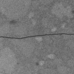
(a) Image $I_{6}$

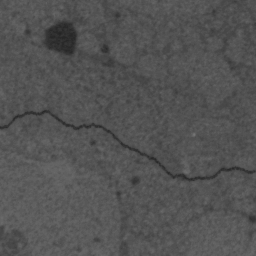
(b) Image $I_{7}$

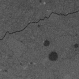
(c) Image $I_{8}$

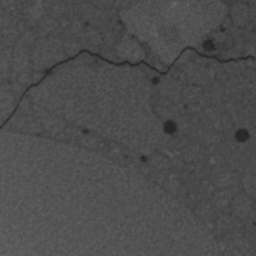
(d) Image $I_{9}$

(e) Image $I_{10}$

Figure 5: 2D slices of five semi-synthetic $250^{3}$ CT input images.

Consider the set of five $250^{3}$ semi-synthetic input images with constant crack width $w=3$, denoted as $I_{6}-I_{10}$ in Figure 5, with $\mathcal{S}=\{1,3,5,10\}$ and the parameter value $g=5$. We set the global threshold $\tau=50$, where the value 50 corresponds to the number of voxels on one edge of $\partial[a_{q},\ b_{q}]^{3}$.

For a $50^{3}$ subimage $A_{q}$, assume that a crack $A_{q}$ intersected with $\partial[a_{q},\ b_{q}]^{3}$ has a rectangular shape of size $50\times w$. Since we would like to control the false negative rate at level $\alpha$, the maximal mesh size $\Delta_{\max}(\alpha)$ from (1) with $\epsilon=0.1$ yields $\Delta_{\max}(0.01)=2$ and $\Delta_{\max}(0.05)=5$.

		Precision	Recall	F1-score
$\Delta=2$	Image $I_{6}$	0.4393939	1.0000000	0.6105263
	Image $I_{7}$	0.3882353	1.0000000	0.5593220
	Image $I_{8}$	0.3870968	0.9729730	0.5538462
	Image $I_{9}$	0.4197531	1.0000000	0.5913043
	Image $I_{10}$	0.3125000	1.0000000	0.4761905
$\Delta=5$	Image $I_{6}$	0.4531250	1.0000000	0.6236559
	Image $I_{7}$	0.3789474	0.9696970	0.5378151
	Image $I_{8}$	0.3913043	0.9729730	0.5581395
	Image $I_{9}$	0.4303797	1.0000000	0.6017699
	Image $I_{10}$	0.3118280	0.9666667	0.4715447

Table 1: Precision, Recall and F1-score of our crack detection method applied to the semi-synthetic input images $I_{6}-I_{10}$.

The recall metric in Table 1 shows that our method controls the false negative rate at level $\alpha$ with the mesh size $\Delta=\Delta_{\max}(\alpha)$. The low precision in Table 1 can be explained by the presence of a large number of tiny thin cracks in images $I_{6}-I_{10}$.

It is evident that setting $\tau$ to match the length of the edge of cubic subimages results in a strategy that prioritizes capturing mid long cracks, leading to high sensitivity. This approach effectively reduces the occurrence of false negatives, a critical aspect in concrete crack detection, by rarely overlooking anomaly regions. However, the pursuit of high sensitivity comes at the expense of precision, as it tends to generate a notable number of false positives. Consequently, while this method focuses on pre-identifying large-scale issues and filtering out noise with minimal computational resources, it lacks the precision required to indicate the exact locations of cracks.

4.2 Real CT images

In images $I_{4}$ and $I_{5}$ from Figure 6, the crack width is not constant. In order to derive the binary image $L_{\mathcal{S}}(I_{j}),j=4,5$, we use a multiscale approach in the Maximal Hessian Entry filter with $\mathcal{S}=\{1,3,5,10\}$. Since the size of the input images is large enough, set $\Delta=3;5$, $g=5;6;10;12$, and the corresponding global threshold $\tau$ equal to the number of voxels on an edge of $\partial[a_{q},\ b_{q}]^{3}$. The results corresponding to $I_{4}$ and $I_{5}$ are shown in Figure 7.

(a) $500^{3}$ input image $I_{4}$

(b) $600^{3}$ input image $I_{5}$

Figure 6: 2D slices of two 3D CT input images of concrete.

(a) Image $I_{4}$

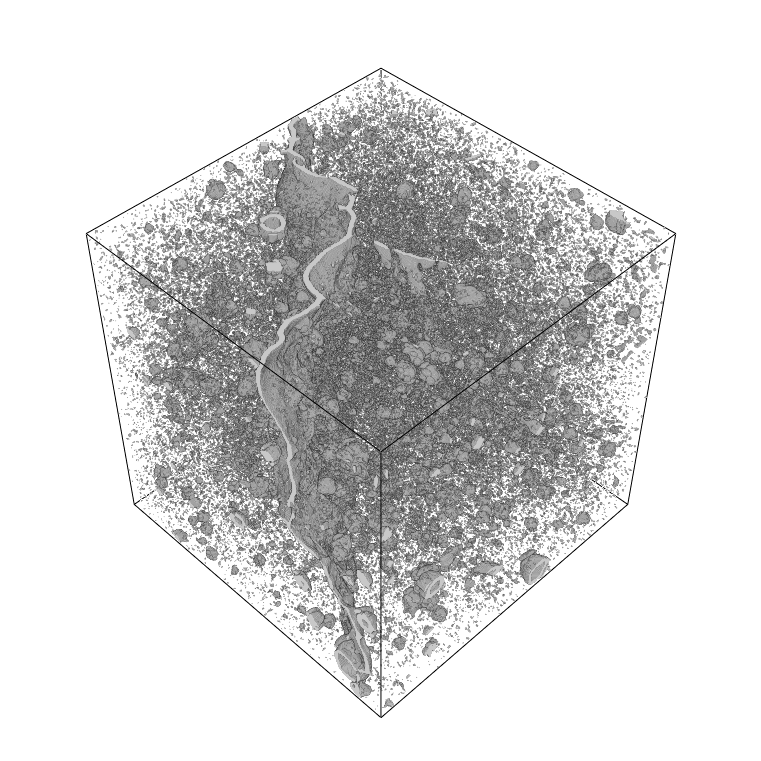
(b) Image $L_{\mathcal{S}}(I_{4})$

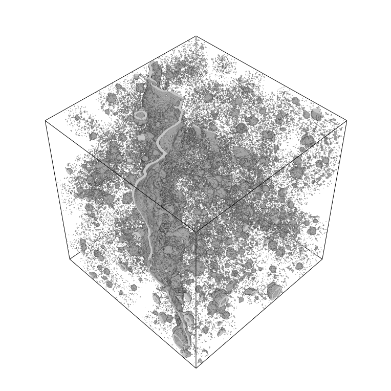
(c) $g=10,\Delta=3$

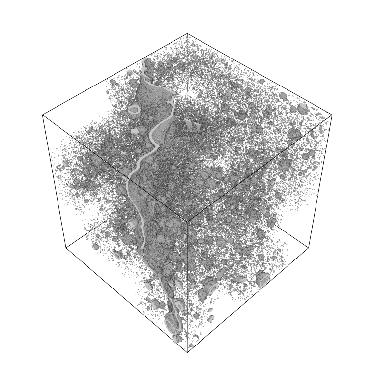
(d) $g=5,\Delta=3$

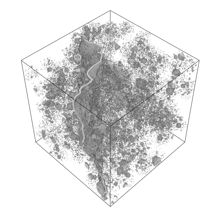
(e) $g=10,\Delta=5$

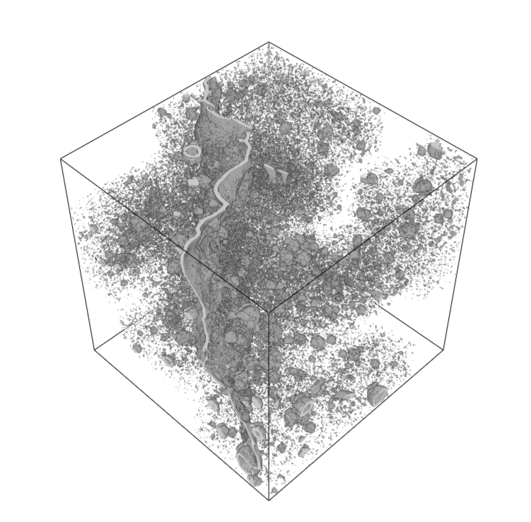
(f) $g=5,\Delta=5$

(g) Image $I_{5}$

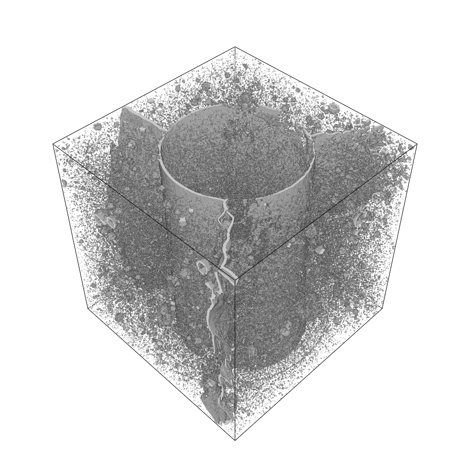
(h) Image $L_{\mathcal{S}}(I_{5})$

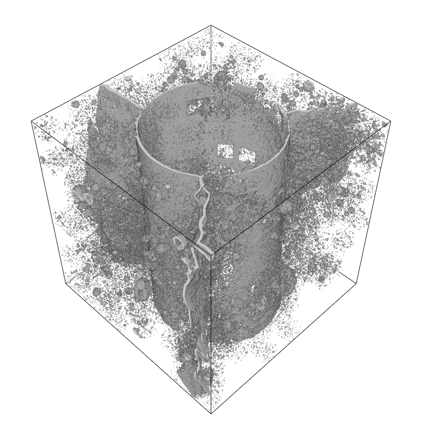
(i) $g=12,\Delta=3$

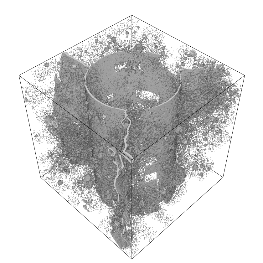
(j) $g=6,\Delta=3$

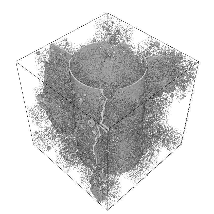
(k) $g=12,\Delta=5$

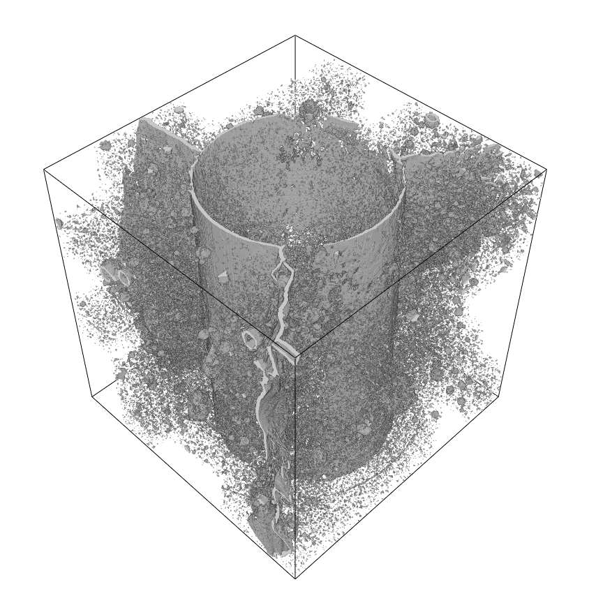
(l) $g=6,\Delta=5$

Figure 7: The input images $I_{4},I_{5}$ and the crack detection results produced by our method.

As the grid lattice get denser (i.e. the mesh size $\Delta$ decreases), it is very likely that our method also captures lots of voxels which apparently do not belong to cracks (high level of false positives). Therefore, the reduction of noise for small $\Delta$ is not significant. However, for higher values of $\Delta$, $(\Delta\geq 5)$, as presented in (e) and (f) in Figure 7, the ratio of FP falls.

These results demonstrate the potential of our method to effectively reduce the amount of noise, eliminating artefacts such as air pores in noisy concrete CT image. By pre-identifying area of a CT image, further statistical inference on their complement will enhance the quality of subsequent exact crack segmentation.

4.3 Run time

The above numerical experiments were conducted on a desktop PC equipped with an Intel(R) Core(TM) i9-10900K CPU running at 3.70 GHz and 128 GB RAM. The procedure comprises two main steps: crack segmentation and the implementation of the DFS algorithm to identify inhomogeneous regions. The highest computational cost is associated with the maximum value of $g$ and the minimum value of $\Delta$. For the $600^{3}$ input image $I_{5}$ in Figure 6, the crack pre-segmentation runtime is approximately 22 seconds, while executing the DFS algorithm with $(g,\Delta)=(12,3)$ takes around 9 seconds. For other pairs $(g,\Delta)$, including $(12,5)$, $(6,3)$, and $(6,5)$, the runtimes are 7 seconds, 4.5 seconds, and 3.6 seconds, respectively. In terms of complexity, our method requires $O(\#W)$ arithmetic operations, where $\#W$ represents the total number of voxels of the input image. To address the computational demands posed by very large-scale real images, we suggest to implement parallel computing, which is well supported by the above algorithms.

5 Conclusions

This paper presents a fast and efficient approach to pre-localize cracks in large CT 3D image of concrete, offering a significant add-on value in computational challenges associated with large-scale input images. It aims to balance the trade-off between the complexity of traditional crack segmentation methods and their effectiveness. The key feature lies in the combination of the Maximal Hessian Entry filter and a DFS-based approach with significantly reduced complexity, being able to deal with large-scale images (eg. $10000^{2}\times 2000$ voxels) within a reasonable time frame.

The numerical experiments show that our method captures the structure of cracks well and avoids misclassification of anomaly regions, which is crucial in materials science application. Additionally, its ability to be combined with slower statistical methods for exact crack segmentation is evident. By significantly reducing the image space to be scanned for a crack, our approach enhances the overall quality crack segmentation for large 3D CT images under acceptable run times.

Last but not least, our approach quantifies the error probability of missing a crack with a given mean width.

6 Acknowledgements

This research was funded by the German Federal Ministry of Education and Research (BMBF) [05M20VUA (DAnoBi)].

References

- [1] T. Barisin, C. Jung, F. Müsebeck, C. Redenbach, and K. Schladitz. Methods for segmenting cracks in 3D images of concrete: A comparison based on semi-synthetic images. Pattern Recognition, 129:108747, 2022.
- [2] Ö. Çiçek, A. Abdulkadir, S. S. Lienkamp, T. Brox, and O. Ronneberger. 3D U-Net: Learning dense volumetric segmentation from sparse annotation. In Lect. Notes Comput. Sc., pages 424–432, 2016. https://doi.org/10.1007/978-3-319-46723-8\_49.
- [3] K. Ehrig, J. Goebbels, D. Meinel, O. Paetsch, S. Prohaska, and V. Zobel. Comparison of crack detection methods for analyzing damage processes in concrete with computed tomography. In DIR 2011-International symposium on digital industrial raidology and computed tomography (Proceedings), number DGZfP-BB 128 (Poster 2), pages 1–8. Deutsche Gesellscahft für Zerstörungsfreie Prüfung eV (DGZfP), 2011.
- [4] S. Even and R. E. Tarjan. Network flow and testing graph connectivity. SIAM journal on computing, 4(4):507–518, 1975.
- [5] A. F. Frangi, W. J. Niessen, K. L. Vincken, and M. A. Viergever. Multiscale vessel enhancement filtering. In W. M. Wells, A. Colchester, and S. Delp, editors, Medical Image Computing and Computer-Assisted Intervention — MICCAI’98, pages 130–137, Berlin, Heidelberg, 1998. Springer Berlin Heidelberg.
- [6] G. L. Golewski. The phenomenon of cracking in cement concretes and reinforced concrete structures: The mechanism of cracks formation, causes of their initiation, types and places of occurrence, and methods of detection - a review. Buildings, 13(3), 2023.
- [7] J. Hopcroft and R. Tarjan. Algorithm 447: efficient algorithms for graph manipulation. Communications of the ACM, 16(6):372–378, 1973.
- [8] C. Jung and C. Redenbach. Crack modeling via minimum-weight surfaces in 3D Voronoi diagrams. Journal of Mathematics in Industry, 13(1):10, 2023.
- [9] C. Jung, C. Redenbach, and K. Schladitz. VoroCrack3d: An annotated data set of 3d CT concrete images with synthetic crack structures, Jan. 2024.
- [10] V. Makogin, D. Nguyen, and E. Spodarev. A statistical method for crack detection in 3D concrete images. Preprint, arXiv:2402.16126, 2024.
- [11] E. Roldán-Pensado. The probability that a convex body intersects the integer lattice in a k-dimensional set. Discrete & Computational Geometry, 47(2):288–300, 2012.
- [12] Y. Sato, C. Westin, A. Bhalerao, S. Nakajima, N. Shiraga, S. Tamura, and R. Kikinis. Tissue classification based on 3D local intensity structures for volume rendering. IEEE Transactions on Visualization and Computer Graphics, 6(2):160–180, 2000.
- [13] C. Sommer, C. N. Straehle, U. Köthe, and F. A. Hamprecht. Ilastik: Interactive learning and segmentation toolkit. In I. S. Biomed. Imaging, pages 230–233, 2011. https://doi.org/10.1109/ISBI.2011.5872394.
- [14] C. R. T. Barisin, K. Schladitz. Riesz networks: scale invariant neural networks in a single forward pass. Journal of Mathematical Imaging and Vision, 66:246–270, 2024.
- [15] R. Tarjan. Depth-first search and linear graph algorithms. SIAM journal on computing, 1(2):146–160, 1972.