Simplicits: Mesh-Free, Geometry-Agnostic, Elastic Simulation

Abstract.

The proliferation of 3D representations, from explicit meshes to implicit neural fields and more, motivates the need for simulators agnostic to representation. We present a data-, mesh-, and grid-free solution for elastic simulation for any object in any geometric representation undergoing large, nonlinear deformations. We note that every standard geometric representation can be reduced to an occupancy function queried at any point in space, and we define a simulator atop this common interface. For each object, we fit a small implicit neural network encoding spatially varying weights that act as a reduced deformation basis. These weights are trained to learn physically significant motions in the object via random perturbations. Our loss ensures we find a weight-space basis that best minimizes deformation energy by stochastically evaluating elastic energies through Monte Carlo sampling of the deformation volume. At runtime, we simulate in the reduced basis and sample the deformations back to the original domain. Our experiments demonstrate the versatility, accuracy, and speed of this approach on data including signed distance functions, point clouds, neural primitives, tomography scans, radiance fields, Gaussian splats, surface meshes, and volume meshes, as well as showing a variety of material energies, contact models, and time integration schemes.

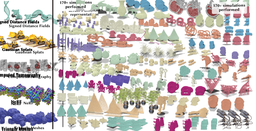
Figure 1. Mesh-free volumetric simulation of objects represented by explicit triangle meshes, point clouds, implicit functions, Computed Tomography volumes, NeRFs, and Gaussian Splats, all produced using our data-free neural fields-based simulation algorithm. Here we show frames from 60 of the 140+ simulations performed.

Description.

1. Introduction

Across visual computing, there is ever-growing use of an incredible variety of 3D representations, from explicit meshes to implicit neural fields, each a source of important and high-fidelity geometric content. Entire databases of implicit shapes, neural or otherwise, are readily available and contain objects ranging from simple polyhedra to wildly complex fractals. One of the great advancements in computer graphics is the ease with which any user, expert or novice, can convincingly render any and all of these geometric representations to display rich 3D scenes. This project (Simplicits) is an attempt to bring the benefits of representation agnostics to elastic simulation.

Functional, robust, feature-rich physics-based elastic simulators are often closely connected to one input geometry type. Once we start to consider other inputs, that bespoke toolchain must change, in potentially complicated ways. Even particle-based methods such as material point method (MPM) and smoothed-particle hydrodynamics (SPH), which reduce surface-to-volume conversion to point sampling, often struggle to resolve intricate boundaries and can exhibit artifacts in the simulated motion.

Simplicits alleviates these issues and provides mesh-free, reduced, physics-based elastic simulation. Simplicits is built upon the observation that any geometric representation is encoded either explicitly or implicitly by an inside-outside (occupancy) function. For most representations, occupancy functions are either trivial or the subject of well-studied algorithms: the sign of the signed-distance function of a mesh, likewise querying an SDF field, fast winding numbers on a point cloud ((Barill et al., 2018)), etc. For NeRFs/Splats and medical scans we extract occupancy from the density field.

Our algorithm is mesh-free at every stage, relying on linear blend skinning (LBS) to characterize the shape-aware/boundary-aware deformation of our object. Skinning weights are represented via a neural field over the object (in $\mathbb{R}^{3}$) and are optimized during training after random initialization. Our approach deviates from standard LBS since we do not explicitly define handle locations on the object. Our skinning weights need not satisfy partition-of-unity or the Kronecker delta properties. Instead, handles are simply transformation matrices applied over the object scaled by skinning weights as described by Benchekroun et al. (2023).

Our method can capture the nuanced behavior of geometrically complex shapes (Figure 2) as well as heterogeneous materials (Figure 15) by using “skinning weights” as a physics-informed deformation basis. Handle transformation DOFs robustly capture large rotations and deformations without artifacts. At runtime, we use Newton’s method to solve for handle matrix values that give an optimal result according to the integration equations.

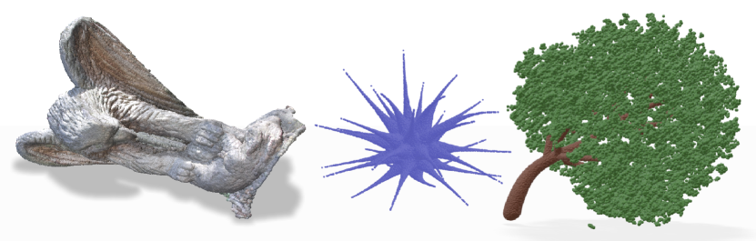
Figure 2. Simulations of point clouds undergoing large deformations. Our method produces shape-aware skinning weights on complex geometries.

To demonstrate the efficacy of Simplicits, we perform a large number of elastodynamic simulations on a myriad of input geometry representations—triangle meshes, signed and unsigned distance functions, neural implicits, NeRFs Gaussian Splats, and medical imagery—all without modifying the algorithm or its parameters. Across these representations, we show results that are volumetric, thin rods or sheets, and shapes that combine all three of these challenging features—again without requiring the algorithm to make any explicit distinction between them. In total this paper features more than 140 simulation results. It is our hope that the generality of this approach helps to make elastodynamic physics simulation a more accessible and enjoyable tool for the greater graphics community, rather than just the expert practitioners.

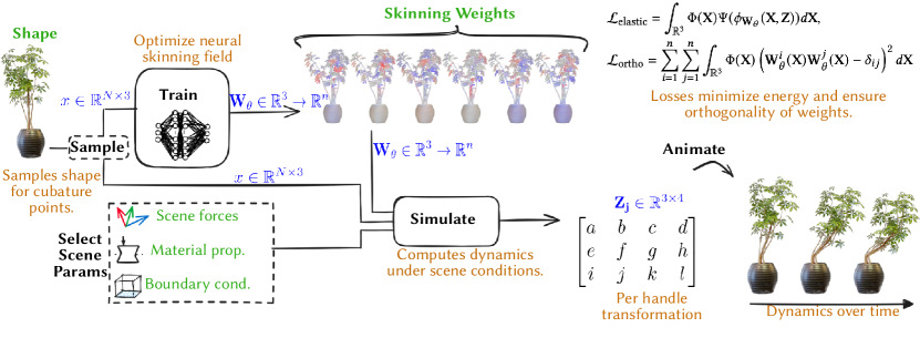
Figure 3. Pipeline overview. First, the skinning weights $\mathbf{W}_{\theta}$ are learned by minimizing the potential and orthogonality losses over randomized deformations ($N$ is the number of samples, and $n$ is the number of skinning handles). Then, given physical material properties and scene conditions, keyframes of transformation-per-handle $\mathbf{Z}_{j}$ are generated, finally combined into an animated object.

2. Related Work

Mesh-Based Methods

Mesh-based elasticity simulation has long been a part of computer graphics (Terzopoulos et al., 1987). The most common variant in use today, for volumetric simulation, is the linear tetrahedral finite element method (Cutler et al., 2002). Since its initial introduction to graphics there have been fundamental improvements in performance (Bargteil et al., 2007; Bouaziz et al., 2014; Macklin et al., 2016), extensions to more complicated phenomena (Bargteil et al., 2007) including contact (Li et al., 2020) and higher-order implementations (Schneider et al., 2019, 2018). In our context, the most important advancements have been made in the geometry processing pipeline that constructs volumetric tetrahedral meshes from surface input. Here robust tools (Hu et al., 2018; Diazzi et al., 2023) enable virtually closed-box simulation of such geometry. However, even broadening the scope of input geometry slightly increases the complexity of the geometry processing and simulation pipelines significantly. For instance, objects with thin features either force volumetric mesh resolutions to be exceedingly high (impractical for many applications) or require special co-dimensional treatments that allow for the inclusion of medial axis geometry (lines for rods and sheets for triangles) into the simulation. Specialized simulators exist for geometry solely constructed from thin primitives (Baraff and Witkin, 2023; Bergou et al., 2008) but, coupling these to volumetric approaches requires non-trivial solutions (Chang et al., 2019; Li et al., 2021).

Embedded Methods

An attractive alternative is embedded methods, which wrap geometry inside of some easily constructable discretization for simulation (Joshi et al., 2007; Longva et al., 2020; Lee et al., 2018), and have even been extended to recent neural representations (Yuan et al., 2022; Xu and Harada, 2022; Garbin et al., 2022). These can produce excellent results, but will naively couple disparate geometric elements embedded in the same element, again necessitating additional algorithmic modifications (Nesme et al., 2009).

Mesh-Free Methods

Alternatively, to simulate complex geometries, one could turn to mesh-free methods, which were first introduced to graphics by Desbrun and Cani (1995). A well-known example is smoothed-particle hydrodynamics (SPH) (Desbrun and Cani, 1996; Peer et al., 2018; Kugelstadt et al., 2021), which requires the connectivity to be updated at every time step. Simplicits, on the other hand, does not need neighborhood information to be queried at runtime. Instead, the deformation gradient and other derived quantities, such as strain and stress, are stored implicitly within a neural field and can be computed anywhere inside the object. The material point method (MPM) has also become popular in graphics in the past decade (Jiang et al., 2016; Wolper et al., 2019; Hu et al., 2019). However, it still requires an explicit background mesh/grid and is prone to numerical artifacts that prevent accurate (quantitatively or qualitatively) simulation of large-scale elastodynamics of complex geometries. Concurrent work for direct simulation of Gaussian Splats (Xie et al., 2023) inherits these limitations. Moving least squares (MLS) formulations were introduced in graphics by Müller et al. (2004) and later extended by Martin et al. (2010) to enable a unified simulation framework for volumetric and co-dimensional objects. However, these methods require extremely dense sampling, which can hurt performance. Also, their interpolation functions do not take shape-aware distance into account and so can couple close but disconnected parts of an object. Faure et al. (2011) introduced a frame-based mesh-free approach, along with pre-computed weight functions to represent object kinematics. This approach is closest to ours technically and philosophically; however, it still requires an explicit boundary for boundary conditions which means it cannot directly take, as input, representations such as Gaussian Splats, while our proposed approach can. Furthermore, the method requires a dense voxelization of the object for computing and storing weight functions which is memory intensive. Another concurrent approach by Feng et al. (2023) develops a voronoi-cell based method for discretizing and simulating NeRFs, however the cell discretizations heavily affect the dynamics and shape-awareness of the simulations. Many other methods have been developed to represent dynamic NeRFs, often using deformation fields (Park et al., 2021; Pumarola et al., 2021), but these are designed to fit supervised observations, rather than to simulate new physical behavior.

Neural Fields for Physics

Leveraging neural networks and neural fields for physics simulation is a fast-growing research area. Chen et al. (2023a) develop a neural simulation technique that can handle infinitely high geometric resolution at a very high simulation cost per time step (often on the order of hours). Other neural techniques pioneered by Fulton et al. (2019) can alleviate some of the issues related to simulation speed via reductions to a nonlinear, neural latent space. Recently, this idea was greatly extended to Continuous-Reduced Order Models (CROM) (Chen et al., 2023b; Chang et al., 2023) which use prior simulation data to generate reduced order models for simulation. While the method by Chang et al. (2023) demonstrates cutting, it relies on the availability of pre-simulated datasets, thus inheriting the geometry processing challenges described above. Additionally, LiCROM requires several hours of training (while ours requires a couple of minutes) and CROM occasionally requires explicit mesh gradients. This again limits their applicability without further algorithmic development. In contrast, our data-free, self-supervised training over a physics-loss is more similar to (Zehnder et al., 2021; Sharp et al., 2023). More specifically, Zehnder et al. (2021) focus on topology optimization over a continuous neural field, while Sharp et al. (2023) optimize a neural network to learn the low-order subspace of an explicit mesh for kinematics. Unfortunately, while this method succeeds in generating kinematic subspaces, it struggles with convergence during dynamics. In contrast, we use data-free, nonlinear skinning weight optimization to learn skinning weight functions over complex objects whether they are represented by an explicit mesh or not.

Skinning Modes

Neural skinning fields using a multi-layer perceptron were originally proposed by Saito et al. (2021) for animated characters and subsequently extended by Mihajlovic et al. (2021) to learn occupancies of articulated characters for collision resolution. Our work on neural skinning fields for dynamics is most related to (Benchekroun et al., 2023; Trusty et al., 2023), a method for skinning-based dynamics simulation. In particular, as a starting point, the skinning eigenmodes by Benchekroun et al. (2023) and extend them in three ways. First, we extend the eigenmode optimization into the nonlinear regime, allowing for more complex energies. Second, in this nonlinear regime, we show that it is possible and preferable to optimize the weights under the assumption of full affine transformations, rather than just the translations of prior work. Next, rather than store skinning weights on a volumetric tetrahedral mesh, we store the weights as neural fields enabling a fully meshless pipeline from beginning to end. Finally, we use this weight field to simulate stable elasto-dynamics using the implicit Euler time integrator (Gast et al., 2015; Martin et al., 2011).

3. Method

Our goal is to construct an integrator for simulating time-varying elastodynamics. Our method will take as input a rest-state object, defined in any geometric representation that supports evaluating an “inside-outside” density $\Phi(x)\in\mathbb{R}^{3}\rightarrow\mathbb{R}$ such that $\Phi(x)=1$ inside the object and $\Phi(x)=0$ outside, possibly with a blurry boundary in-between. Our output will be a set of neural fields that encode skinning weights suitable for dynamics simulation (Figure 3).

3.1. Implicit Time Integration

We start with the deformation map $\mathbf{x}=\phi(\mathbf{X},\mathbf{z}(t))$, where $\mathbf{X}\in\mathbb{R}^{3}$ is a point in reference space and $\mathbf{x}\in\mathbb{R}^{3}$ is its deformed position according to $\mathbf{z}(t)$, a time-varying vector of as-yet unspecified degrees-of-freedom (DOFs). If $\phi$ is a linear function with respect to $\mathbf{z}$, then we can discretize standard implicit time integration as the following optimization problem

(1) $$\mathbf{z}_{t+1}=\underset{\mathbf{z}}{\arg\min}\frac{1}{2}\|\mathbf{z}-\tilde{\mathbf{z}_{t}}\|^{2}_{\mathbf{M}}+h^{2}E_{\textrm{pot}}(\mathbf{z}),$$

where $\mathbf{z}_{t+1}$ are the integrated DOFs for the next time step, $\|\cdot\|^{2}_{\mathbf{M}}$ is the squared norm weighted by an appropriate mass matrix, $h$ is the simulation time step, $E_{\textrm{pot}}$ is the elastic potential energy of the simulated object and $\tilde{\mathbf{z}}_{t}$ is the standard first order predictor for $\mathbf{z}$. This formulation can be augmented with constraints and penalty springs for maintaining fixed or moving boundary conditions along with barrier functions to handle contact and then solved using standard Newton-based methods  (Nocedal and Wright, 2006; Li et al., 2020). Our goal is to choose an appropriate set of DOFs that are both expressive enough to generate compelling simulation results and amenable to a neural representation for adaptive generality.

3.2. Degrees-of-Freedom

As previously noted, simply parameterizing $\phi$ as a pure neural nonlinear function typically fails for dynamics (Sharp et al., 2023). Standard FEM shape functions satisfy linearity, but require explicit polyhedra for construction. Particles with extrapolating shape functions are more general, but incur modeling and numerical challenges as discussed in Section 2. Blended affine transformations, or skinning handles, are promising solution, offering easy numerical integration and accurate modeling of elastic phenomena. Accordingly, we parameterize our deformation map, $\phi$ using linear blend skinning

(2) $$\phi(\mathbf{X},\mathbf{z})=\mathbf{X}+\sum_{j=1}^{n}\mathbf{W}_{\!j}(\mathbf{X})\mathbf{Z}_{j}\begin{bmatrix}\mathbf{X}\\ 1\end{bmatrix}$$

where $n$ is the number of skinning handles, $\mathbf{W}_{\!j}(\mathbf{X})\in\mathbb{R}^{3}\rightarrow\mathbb{R}$ is the spatially varying scalar shape function associated with handle $j$, $\mathbf{Z}_{j}\in\mathbb{R}^{3\times 4}$ is the $j^{th}$ skinning handle. The vector $\mathbf{z}$ of DOFs is formed by flattening the stacked handle transforms: $\mathbf{z}=\text{flat}(\mathbf{Z})\in\mathbb{R}^{12n}$. In the subsequent text, we assume that $\mathbf{z}\in\mathbb{R}^{12n}$ and $\mathbf{Z}\in\mathbb{R}^{(3\times 4)\times n}$ are interchangeable, with implicit conversion between them.

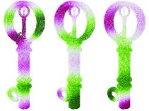
Figure 4. Trained skinning weights.

While previous work stores the skinning shape functions $\mathbf{W}\in\mathbb{R}^{3}\rightarrow\mathbb{R}^{n}$ on an explicit volumetric mesh (Benchekroun et al., 2023), we instead store these functions as a vector-valued continuous neural field $\mathbf{W}_{\theta}\in\mathbb{R}^{3}\rightarrow\mathbb{R}^{n}$, removing the need for any explicit geometric scaffolding, yielding a purely meshless discretization during training and at runtime.

3.3. Meshless Integration in Space

Before we address the training of these neural fields, we must first describe the evaluation of integral quantities over the domain. Both our mass matrix and potential energies are quantities integrated over the domain of the geometry

(3) $$\mathbf{M}=\int_{\Omega}\rho\mathbf{J}(\mathbf{X})^{T}\mathbf{J}(\mathbf{X})d\Omega\qquad E_{\textrm{pot}}=\int_{\Omega}\Psi(\phi(\mathbf{X}))d\Omega,$$

where $\Omega$ is the interior domain of our object in the undeformed reference space, $\rho\in\mathbb{R}$ is its physical density, $\mathbf{J}=\nabla_{\!\mathbf{z}}\phi$ is the Jacobian function of the deformation map evaluated at $\mathbf{X}\in\Omega$, and $\Psi$ is the strain energy density function (Kim and Eberle, 2020). We note that since the deformation map $\phi$ is linear with respect to the DOFs $\mathbf{z}$, the Jacobian $\mathbf{J}\in\mathbb{R}^{3\times 12n}$ and the mass matrix $\mathbf{M}\in\mathbb{R}^{12n\times 12n}$ are constant.

Inserting our occupancy density into any such integral yields the general from

(4) $$G=\int_{\mathbb{R}^{3}}\Phi(\mathbf{X})g(\mathbf{X})d\mathbf{X},$$

where $g$ is the quantity to be integrated, as in Equation 3. We evaluate this via Monte Carlo integration, sampling the domain of the object.

3.4. Neural Skinning Field Loss

Good skinning weights accurately capture large, physically plausible rotations and deformations of an object, even with a limited number of handles. We seek to fit an implicit weight function $\mathbf{W}$ with these properties; i.e. we train the parameters $\theta$ of a neural network $\mathbf{W}_{\theta}$:

(5) $$\theta^{*}=\underset{\theta}{\arg\min}\ \lambda_{\textrm{elastic}}\mathcal{L}_{\textrm{elastic}}+\lambda_{\textrm{ortho}}\mathcal{L}_{\textrm{ortho}}.$$

The result is a fitted implicit weight function $\mathbf{W}_{\theta^{*}}\in\mathbb{R}^{3}\rightarrow\mathbb{R}^{n}$ for the shape, which smoothly captures large nonlinear deformations.

Physical-Plausibility

Material-aware and spatial-aware deformations have low elastic potential energy (Equation 3), while undesirable nonsensical deformations have very high elastic energy. Accordingly, we seek weights that minimize the elastic energy for any random set of handle transformations

(6) $$\mathcal{L}_{\textrm{elastic}}=\int_{\mathbb{R}^{3}}\Phi(\mathbf{X})\Psi(\phi_{\mathbf{W}_{\theta}}(\mathbf{X},\mathbf{Z}))d\mathbf{X},$$

where in-practice small transformations $\mathbf{Z}$ are randomly sampled from $\mathbf{Z}$ during training, as described later in Section 4.

Orthogonality

Unfortunately, naively minimizing $\mathcal{L}_{\textrm{elastic}}$ immediately collapses to a trivial solution, with all handles encoding a constant weight, limiting the model to rigid motions. This could be mitigated in a “supervised” manner, by requiring the skinning weights to reproduce some dataset of motions, but such datasets are rarely available in practice. Instead, we adopt a data-free approach that additionally seeks weights that are mutually orthonormal under the inner product on scalar functions $\int\!f(x)g(x)dx$, which amounts to minimizing

(7) $${\color[rgb]{0,0,0}\mathcal{L}_{\textrm{ortho}}=\sum_{i=1}^{n}\sum_{j=1}^{n}\int_{\mathbb{R}^{3}}\Phi(\mathbf{X})\left(\mathbf{W}_{\theta}^{i}(\mathbf{X})\mathbf{W}_{\theta}^{j}(\mathbf{X})-\delta_{ij}\right)^{2}d\mathbf{X},}$$

where $i$ and $j$ are handle indices, and $\delta_{ij}$ is the Kronecker delta.

4. Implementation

4.1. Network Architecture and Training

We represent the skinning weight function $\mathbf{W}$ as a small neural network per-object $\mathbf{W}_{\theta}:\mathbb{R}^{3}\to\mathbb{R}^{n}$ with parameters $\theta$, which takes spatial coordinates as input and outputs skinning weights at the point. Please see the supplemental material for a detailed listing of all parameters.

Architecture

We choose $\mathbf{W}_{\theta}$ to be a small multi-layer perceptron (MLP), with ELU activation functions on hidden layers. The size of the network depends on the complexity of the problem; 9 hidden layers is typical, we use width 64 for all objects. For the sake of parameter scaling, all inputs are normalized to have length-scale $\approx\!1$ before network evaluation. Unlike classic skinning formulations, where the weights $\mathbf{W}$ are defined as a partition of unity, or at least positive, we find it effective in practice to leave $\mathbf{W}$ unconstrained in $\mathbb{R}^{n}$, and use them as a reduced subspace, akin to skinning eigenmodes (Benchekroun et al., 2023).

Training

We fit $\mathbf{W}_{\theta}$ for each object by minimizing the elastic and orthogonality losses (Equation 5) using the Adam optimizer (Kingma and Ba, 2014) with a linearly scheduled learning rate. For each training iteration, we sample a batch of random transformations $\mathbf{Z}$ for each handle, as well as cubature points to evaluate spatial integrals (Section 3.3). The transformation matrices $\mathbf{Z}$ are drawn elementwise from $\mathbf{Z}\!\sim\!\mathcal{N}(\mu,0)$. We find that $\mu=0.1$ is effective for unit-scaled objects, and that training on relatively small unconstrained perturbations yields weights which generalize well to large nonlinear deformations. We schedule the elastic energy as $\Psi=(1-\alpha)\Psi_{\textrm{linear elastic}}+\alpha\Psi_{\textrm{neohookean}}$, where $\alpha$ goes $0\to 1$ during training, because linear elasticity has stable gradients even for randomly initialized weights, while Neohookean elasticity improves large-deformation behavior of the final weights.

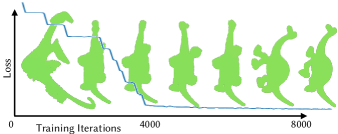
Figure 5. Simulation quality improves during neural skinning weight training.

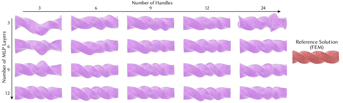
Figure 6. Increasing the degrees of freedom in our simulation (number of skinning handles $n$) and the capacity of the neural skinning function (number of MLP hidden layers) both increase the expressivity of the method. Note that network capacity must be sufficient to match the DOFs. Having 3 layers with 24 handles is insufficient for complex deformations. We use nonlinear Neohookean energy for these deformations.

4.2. Time-Stepping

Once the skinning weights $\mathbf{W}_{\theta}$ have been fit, we timestep the simulation by solving Equation 1 using standard projected Newton’s method with a line search. For fast simulation we evaluate integrals at a fixed set of sample points drawn once in the rest space as a preprocess. We emphasize that with this setup, our method does not require evaluating the neural network at all within the physics time-stepping loop, just once as a preprocess to compute weights and their derivatives at sample points—this is a key reason for the speed and robustness of our method. If desired, the neural skinning weights can later be evaluated at any point in space to query the smooth simulated deformation. Our approach is compatible with any hyperelastic material, and the energy used for simulation need not match the energy used for training. The majority of our examples use the stable Neohookean model (Kim and Eberle, 2020).

4.3. Representation-Specific Concerns

A primary goal of this work is to simulate on a very wide variety of representations our experiments include meshes, NeRFs, CT scans, Gaussian Splats, and more. An in-depth introduction of each of these representations is beyond the scope of this document, but our general procedure is the same for all representations. We define an occupancy function $\Phi$ such as an inside-outside test on a mesh, thresholded NeRF density, or clipped Houndsfield units in a CT scan, as well as specifying a bounding domain for the rest geometry, and any needed physical parameters like density and stiffness. Spatial samples to evaluate integrals can come directly from the geometry, such as fast mesh sampling and particle subsets from particle-based methods, or be generated by rejection sampling, taking uniformly random points within the domain where $\Phi(\mathbf{X})>0$.

After simulation, one generally needs to render or otherwise interact with the deformed object. For explicit representations such as meshes and particles, our continuous forward deformation field (Equation 2) can be queried at any point to translate rest points to the deformed location. If needed, we can also read off local rotations, e.g. to rotate the orientation of Gaussian Splat particles. Implicit representations such as NeRFs are more difficult, as volumetric rendering generally requires the reverse map taking points in deformed space back to the rest space; prior work has tackled this e.g. by adaptively tracing curved rays (Seyb et al., 2019). We do not present any new solutions to this challenge in this work; we sidestep it on a case-by-case basis by point sampling or extracting meshes for visualization only—this is an important problem for future research.

4.4. Software and Fast Computation

Table 1. Selected timing results. See supplements for details.

Name	Figure	Training	Sim Step
Mesh monkey	Figure 1	180 sec	51 ms
SDF key	Figure 4	886 sec	107 ms
Gaussian Splat lego	Figure 13	5550 sec	74 ms

We implement our method in Pytorch (Paszke et al., 2017), running entirely on the GPU. Code will be made available upon acceptance to facilitate adoption and clarify details. All experiments and timings are evaluated on a single RTX 3070. Spatial derivatives are evaluated via finite differences, and training gradients are evaluated with standard backpropagation. For time stepping, we find that assembling Hessians and gradients for Newton steps via automatic differentiation is excessively expensive, and instead assemble them with explicit analytical expressions, albeit still in pure Pytorch code. Visualizations are rendered with various packages including Blender, Polyscope, and Houdini as appropriate for each experiment.

5. Evaluation

We use standard elastic simulation benchmarks on a prismatic bar to assess the accuracy of our method, ablate its components, and compare to alternatives.

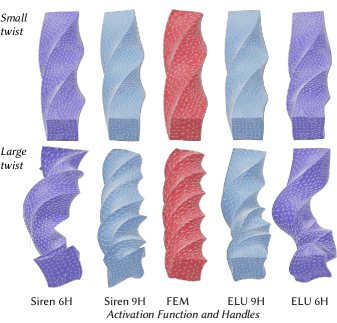
Figure 7. Comparing ELU vs. SIREN (Sitzmann et al., 2020) activation functions on a large deformation. We experimentally find that using ELU activations, our simulation satisfies boundary conditions more strictly than when using SIREN.

Validation

In Figure 6, we compare a twisted bar simulated with our method to a ground-truth solution from linear tetrahedral FEM. Accuracy improves as we increase the number of handles and capacity of the MLP. Figure 9 uses the same setup to ablate the use of the Neohookean energy during training, as well as sampling full handle transformations rather than just translations. Both of these factors introduce increased nonlinear rotation into the training procedure, and as-expected the resulting weights modestly improve accuracy when the bar is in a highly-twisted near-buckling state. Figure 5 shows the training dynamics and loss curve. Although the loss does not decrease much after 5000 iterations, additional training still visually improves the quality of the simulation. Figure 7 compares the choice of activation function in the neural network. We find that ELU activation handles boundary conditions better than SIREN ((Sitzmann et al., 2020)).

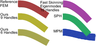
Figure 8. A cantilever bar comparison between a reference linear-tetrahedral, Corotational FEM beam, our method with 6 and 9 handles, Fast Skinning Eigenmodes (Benchekroun et al., 2023) with 10 handles, SPH (Kugelstadt et al., 2021) with 5582 particles, and MPM (Hu et al., 2019) with 5000 particles and initial grid density of 10. Notice ours matches Fast Skinning Eigenmodes very closely andf exhibits similar numerical coarsening due to reduction when compared to FEM. Simulations are run for 300 steps with timestep $0.01\unit{s}$, with young’s modulus $5e6\unit{Pa}$, poisson ratio $0.45$, density $1000\unit{kg\per m^{3}}$ using corotational linear elastic material.

Comparisons

In Figure 8, we show our method generates results that are as comparable to reference FEM as Fast Skinning Eigenmodes (Benchekroun et al. (2023)) and more than other mesh-free approaches such as SPH ((Peer et al., 2018)) and MPM ((Jiang et al., 2016), as implemented in (Hu et al., 2019)) with a moderate number of handles. Figure 12 likewise compares behavior under sharp contacts.

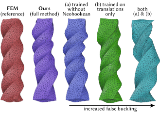
Figure 9. An ablation study, on a square bar pinned at the top and twisted at the bottom. Our full method uses the nonlinear Neohookean energy during training, as well as sampling full transformations. Compared to an FEM reference solution (red), removing either component worsens accuracy.

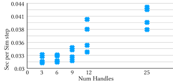
Figure 10. Plotting average time (in ms) per sim step as the number of DOFs increases. Time increases super-linearly due to the dense linear solve in Newton’s Method.

Scaling

We observe that training cost depends mainly on the network size rather than the number of handle degrees of freedom. The supplementary table of 144 experiments shows the scaling of training cost as a function of network width and depth. At simulation time, the dense Newton solves in backward Euler time integration lead to super-linear scaling in the number of handle degrees of freedom (see Figure 10), though, timesteps generally remain interactive even with many handles.

Other Ablations

Our training is robust to moderate hyperparameter adjustments in most cases. For example, training on a linear elastic material without an elastic energy scheduler (shown in Figure 9 (a)) we can achieve visually appealing deformations when simulating a nonlinear material. However, incorporating physics-based energy during training along with the orthogonality term is essential. Training with physics illicits a physics-based response during the simulation as shown in Figure 11.

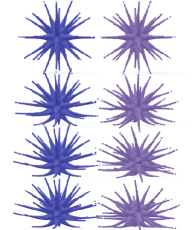
Figure 11. Left: Trained without $\mathcal{L}_{\textrm{elastic}}$ loss. Right: Trained with $\mathcal{L}_{\textrm{elastic}}$.

Another hyperparameter is the learning rate scheduler, which is optional when using smaller learning rates and more steps, but necessary when starting with a larger learning rate for faster convergence. We generally avoid tuning hyperparameters per-object in order to show that a common set of parameters is effective in a wide range of settings, with a few exceptions for ablation experiments and particularly large-scale or complex objects.

6. Results

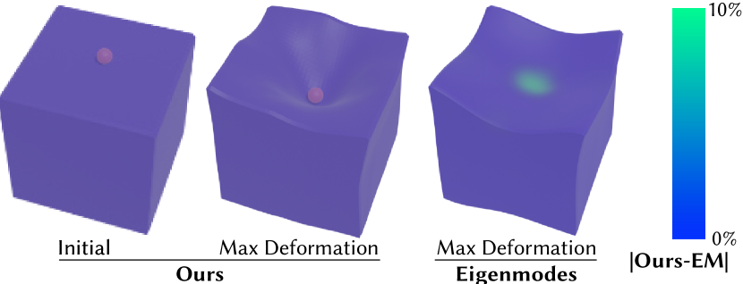
Figure 12. Despite greatly reduced space, our simulations are surprisingly responsive to contacts, which were not seen during the training procedure. For the same number of modes (10), mesh-based eigenmodes fail to capture the sharp nature of the contact. We plot displacement error relative to mesh bounding box diagonal.

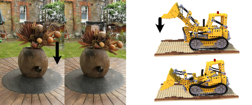
Figure 13. Gaussian splat reconstructions (Kerbl et al., 2023), simulated with gravity (left) and free fall of an object (right). Zoom for details.

To show the broad applicability of simulation with Simplicits, we demonstrate elastic simulations across a wide variety of representations and data sources. Please see the supplemental material for a listing of configurations for all experiments, and two videos giving an overview as well as an extended catalog of results.

Meshes

To begin, we show simulations on standard triangle and tetrahedral meshes with occupancy encoded via a signed distance function (Figure 1, Figure 9). These are well-studied in prior simulation methods, though our approach removes assumptions about element quality or mesh cleanness which may be difficult to meet with in-the-wild data, and offers a unified framework applicable to non-mesh data as well.

Signed Distance Functions

Signed-distance functions (with occupancy encoded as a scalar field) are an increasingly popular shape representation, both as artist-constructed analytical functions and learned neural fields. We simulate the entire dataset of SDFs from Takikawa et al. (2022) under gravity and ground contact (Figure 1, supplemental video). Our adaptive neural field and sampling procedure captures even thin features and codimensional effects (Figure 16).

Point Clouds

Our method trivially applies to point clouds (encoded via  Barill et al. (2018)’s fast winding numbers), interpreting the points as set of samples from the support of $\Phi$, as shown in Figure 2. The toppling Eagle is a 3D-scanned statue point cloud.

NeRF

Neural radiance fields (Mildenhall et al., 2020) have emerged as a powerful paradigm for reconstruction and machine learning, but working with the resulting content afterwards can be difficult compared to explicit methods. Simplicits can be applied directly to NeRF representations (Tancik et al., 2023)  (where occupancy is encoded as a density field), even those from recent generative AI systems (Lin et al., 2023) (Figure 17, supplemental video).

Gaussian Splats

Point splat-based rendering has a long history in computer graphics, and the Gaussian Splat formulation has recently proven to be compelling choice for realtime rendering of reconstructed scenes (Kerbl et al., 2023). Directly simulating Gaussian Splat particles with our method offers fast and high-quality simulations directly on reconstructed data (Figure 13).

Medical Imaging

Beyond computer graphics, simulating medical data is deeply important for health applications, but the challenges of real-world scan data mean off-the-shelf simulators are rarely applicable. We show that Simplicits can be directly applied to meaningful simulations on real CT scan data simply by thresholding the Hounsfield unit for our inside-outside density function $\Phi$. Our results include a bladder from (Kirk et al., 2016) with a contact impact (Figure 14), and a skull and brain from (National Library of Medicine, 2005) colliding with a ground plane under gravity (Figure 15).

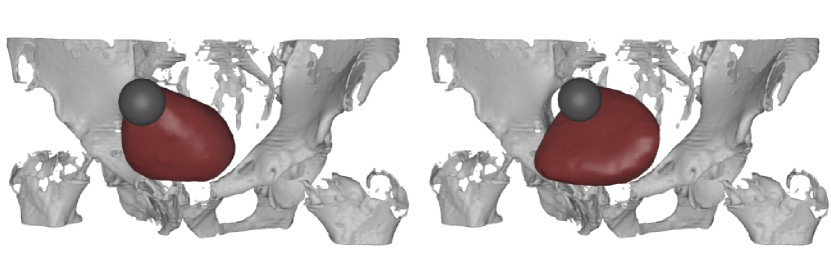
Figure 14. A simulated nonlinear contact on a CT-scanned bladder.

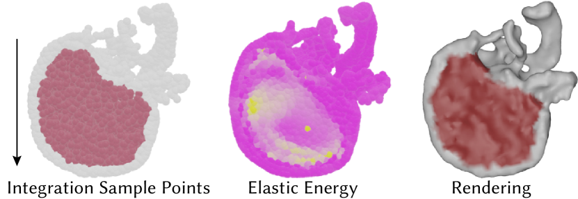
Figure 15. A simulated deformation of a soft brain and stiff skull hitting the floor, directly from CT-scanned geometry.

More results

We demonstrate our method on a large variety of objects ranging from thin ribbons in Figure 16 to highly intricate Gaussian Splatting and NeRFs scenes in Figure 13 and Figure 17. Our method can handle large non-linear deformations and deformations from contact as shown in Figure 12. We demonstrate shape-aware simulations on pointclouds in Figure 2.

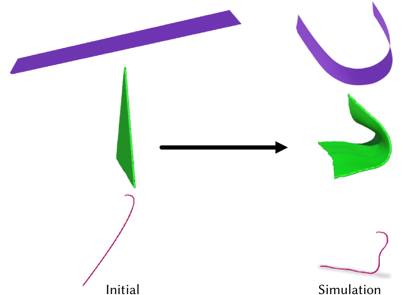
Figure 16. Simulation of thin SDF sheets and strands under gravity and ground collisions.Please see supplemental video for details.

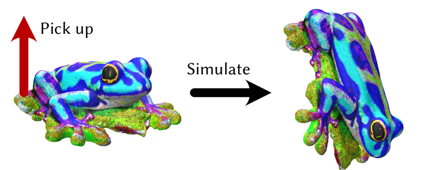
Figure 17. Simulation of a NeRF frog, generated with Magic3D (Lin et al., 2023). See the supplemental video for details.

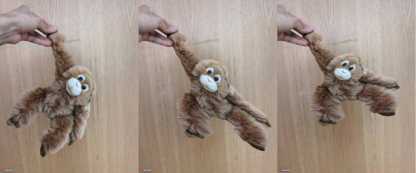
Figure 18. We show preliminary results for simulating elastodynamics in a 2D image. The object is segmented using MIDAS monocular depth (Ranftl et al., 2022) and occluded regions are in-painted using Adobe Firefly.

7. Conclusion

We demonstrate Simplicits, a new approach for deformable elastic simulation which is mesh-free, data-free, efficient, and most-importantly agnostic to the underlying 3D representation. We have used our method to generate simulations on a breadth of inputs all using the same framework, ranging from CT scans to Gaussian splats to neural implicit objects to triangle meshes, resulting in 140+ simulated outputs in total.

Limitations and Future Work

Our neural implicit skinning weight field is fit individually for each object as a pre-processes. Training times are already modest, but could likely be greatly accelerated via grid-based networks which fit similar fields at nearly interactive speeds (Müller et al., 2022).

Although we demonstrate heterogeneous stiffness on several examples (beam Figure 9, skull Figure 15, ficus Figure 13), training convergence may be a challenge for objects with complex and highly-variable layered stiffness distributions.

In implicit volumetric representations such as NeRFs, rendering from the forward deformation map is nontrivial; future work could address this with invertible deformation representations or deformation-aware rendering schemes (Seyb et al., 2019). More broadly, the basic Simplicits paradigm could be extended to additional simulated phenomena such as high-frequency secondary effects, fracture, articulated linkages, or extended to other applications in visual computing, Figure 18 shows a preliminary result to image editing.

- (1)
- Baraff and Witkin (2023) David Baraff and Andrew Witkin. 2023. Large steps in cloth simulation. In Seminal Graphics Papers: Pushing the Boundaries, Volume 2. 767–778.
- Bargteil et al. (2007) Adam W Bargteil, Chris Wojtan, Jessica K Hodgins, and Greg Turk. 2007. A finite element method for animating large viscoplastic flow. ACM transactions on graphics (TOG) 26, 3 (2007), 16–es.
- Barill et al. (2018) Gavin Barill, Neil Dickson, Ryan Schmidt, David I.W. Levin, and Alec Jacobson. 2018. Fast Winding Numbers for Soups and Clouds. ACM Transactions on Graphics (2018).
- Benchekroun et al. (2023) Otman Benchekroun, Jiayi Eris Zhang, Siddhartha Chaudhuri, Eitan Grinspun, Yi Zhou, and Alec Jacobson. 2023. Fast Complementary Dynamics via Skinning Eigenmodes. arXiv:cs.GR/2303.11886
- Bergou et al. (2008) Miklós Bergou, Max Wardetzky, Stephen Robinson, Basile Audoly, and Eitan Grinspun. 2008. Discrete elastic rods. In ACM SIGGRAPH 2008 papers. 1–12.
- Bouaziz et al. (2014) Sofien Bouaziz, Sebastian Martin, Tiantian Liu, Ladislav Kavan, and Mark Pauly. 2014. Projective dynamics: fusing constraint projections for fast simulation. ACM Transactions on Graphics (TOG) 33, 4 (2014), 154.
- Chang et al. (2019) Jumyung Chang, Fang Da, Eitan Grinspun, and Christopher Batty. 2019. A unified simplicial model for mixed-dimensional and non-manifold deformable elastic objects. Proceedings of the ACM on Computer Graphics and Interactive Techniques 2, 2 (2019), 1–18.
- Chang et al. (2023) Yue Chang, Peter Yichen Chen, Zhecheng Wang, Maurizio M. Chiaramonte, Kevin Carlberg, and Eitan Grinspun. 2023. LiCROM: Linear-Subspace Continuous Reduced Order Modeling with Neural Fields. arXiv:cs.GR/2310.15907
- Chen et al. (2023a) Honglin Chen, Rundi Wu, Eitan Grinspun, Changxi Zheng, and Peter Yichen Chen. 2023a. Simulating Physics with Implicit Neural Spatial Representations. In International Conference on Machine Learning.
- Chen et al. (2023b) Peter Yichen Chen, Jinxu Xiang, Dong Heon Cho, Yue Chang, G A Pershing, Henrique Teles Maia, Maurizio M Chiaramonte, Kevin Thomas Carlberg, and Eitan Grinspun. 2023b. CROM: Continuous Reduced-Order Modeling of PDEs Using Implicit Neural Representations. In The Eleventh International Conference on Learning Representations. https://openreview.net/forum?id=FUORz1tG8Og
- Cutler et al. (2002) Barbara Cutler, Julie Dorsey, Leonard McMillan, Matthias Müller, and Robert Jagnow. 2002. A procedural approach to authoring solid models. ACM Transactions on Graphics (TOG) 21, 3 (2002), 302–311.
- Desbrun and Cani (1995) Mathieu Desbrun and Marie-Paule Cani. 1995. Animating soft substances with implicit surfaces. In Proceedings of the 22nd Annual Conference on Computer Graphics and Interactive Techniques (SIGGRAPH ’95). Association for Computing Machinery, New York, NY, USA, 287–290. https://doi.org/10.1145/218380.218456
- Desbrun and Cani (1996) Mathieu Desbrun and Marie-Paule Cani. 1996. Smoothed particles: a new paradigm for animating highly deformable bodies. In Proceedings of the Eurographics Workshop on Computer Animation and Simulation ’96. Springer-Verlag, Berlin, Heidelberg, 61–76.
- Diazzi et al. (2023) Lorenzo Diazzi, Daniele Panozzo, Amir Vaxman, and Marco Attene. 2023. Constrained Delaunay Tetrahedrization: A Robust and Practical Approach. ACM Transactions on Graphics (TOG) 42, 6 (2023), 1–15.
- Faure et al. (2011) François Faure, Benjamin Gilles, Guillaume Bousquet, and Dinesh K Pai. 2011. Sparse meshless models of complex deformable solids. In ACM transactions on graphics (TOG), Vol. 30. ACM, 73.
- Feng et al. (2023) Yutao Feng, Yintong Shang, Xuan Li, Tianjia Shao, Chenfanfu Jiang, and Yin Yang. 2023. PIE-NeRF: Physics-based Interactive Elastodynamics with NeRF. arXiv:cs.CV/2311.13099
- Fulton et al. (2019) Lawson Fulton, Vismay Modi, David Duvenaud, David Levin, and Alec Jacobson. 2019. Latent-space Dynamics for Reduced Deformable Simulation.
- Garbin et al. (2022) Stephan J Garbin, Marek Kowalski, Virginia Estellers, Stanislaw Szymanowicz, Shideh Rezaeifar, Jingjing Shen, Matthew Johnson, and Julien Valentin. 2022. VolTeMorph: Realtime, Controllable and Generalisable Animation of Volumetric Representations. arXiv preprint arXiv:2208.00949 (2022).
- Gast et al. (2015) Theodore F. Gast, Craig Schroeder, Alexey Stomakhin, Chenfanfu Jiang, and Joseph M. Teran. 2015. Optimization Integrator for Large Time Steps. IEEE Transactions on Visualization and Computer Graphics 21, 10 (2015), 1103–1115. https://doi.org/10.1109/TVCG.2015.2459687
- Hu et al. (2019) Yuanming Hu, Tzu-Mao Li, Luke Anderson, Jonathan Ragan-Kelley, and Frédo Durand. 2019. Taichi: a language for high-performance computation on spatially sparse data structures. ACM Transactions on Graphics (TOG) 38, 6 (2019), 1–16.
- Hu et al. (2018) Yixin Hu, Qingnan Zhou, Xifeng Gao, Alec Jacobson, Denis Zorin, and Daniele Panozzo. 2018. Tetrahedral Meshing in the Wild. ACM Trans. Graph. 37, 4, Article 60 (July 2018), 14 pages. https://doi.org/10.1145/3197517.3201353
- Jiang et al. (2016) Chenfanfu Jiang, Craig Schroeder, Joseph Teran, Alexey Stomakhin, and Andrew Selle. 2016. The material point method for simulating continuum materials. In ACM SIGGRAPH 2016 Courses (SIGGRAPH ’16). Association for Computing Machinery, New York, NY, USA, Article 24, 52 pages. https://doi.org/10.1145/2897826.2927348
- Joshi et al. (2007) Pushkar Joshi, Mark Meyer, Tony DeRose, Brian Green, and Tom Sanocki. 2007. Harmonic coordinates for character articulation. ACM transactions on graphics (TOG) 26, 3 (2007), 71–es.
- Kerbl et al. (2023) Bernhard Kerbl, Georgios Kopanas, Thomas Leimkühler, and George Drettakis. 2023. 3D Gaussian Splatting for Real-Time Radiance Field Rendering. ACM Transactions on Graphics 42, 4 (July 2023). https://repo-sam.inria.fr/fungraph/3d-gaussian-splatting/
- Kim and Eberle (2020) Theodore Kim and David Eberle. 2020. Dynamic deformables: implementation and production practicalities. In ACM SIGGRAPH 2020 Courses. 1–182.
- Kingma and Ba (2014) Diederik P Kingma and Jimmy Ba. 2014. Adam: A method for stochastic optimization. arXiv preprint arXiv:1412.6980 (2014).
- Kirk et al. (2016) Shanah Kirk, Yueh Lee, Fabiano R. Lucchesi, Natalia D. Aredes, Nicholas Gruszauskas, James Catto, Kimberly Garcia, Rose Jarosz, Vinay Duddalwar, Bino Varghese, Kimberly Rieger-Christ, and John Lemmerman. 2016. The Cancer Genome Atlas Urothelial Bladder Carcinoma Collection (TCGA-BLCA). https://doi.org/10.7937/K9/TCIA.2016.8LNG8XDR
- Kugelstadt et al. (2021) Tassilo Kugelstadt, Jan Bender, José Antonio Fernández-Fernández, Stefan Rhys Jeske, Fabian Löschner, and Andreas Longva. 2021. Fast corotated elastic SPH solids with implicit zero-energy mode control. Proceedings of the ACM on Computer Graphics and Interactive Techniques 4, 3 (2021), 1–21.
- Lee et al. (2018) Minjae Lee, David Hyde, Michael Bao, and Ronald Fedkiw. 2018. A skinned tetrahedral mesh for hair animation and hair-water interaction. IEEE transactions on visualization and computer graphics 25, 3 (2018), 1449–1459.
- Li et al. (2020) Minchen Li, Zachary Ferguson, Teseo Schneider, Timothy Langlois, Denis Zorin, Daniele Panozzo, Chenfanfu Jiang, and Danny M. Kaufman. 2020. Incremental potential contact: intersection-and inversion-free, large-deformation dynamics. ACM Trans. Graph. 39, 4, Article 49 (aug 2020), 20 pages. https://doi.org/10.1145/3386569.3392425
- Li et al. (2021) Minchen Li, Danny M. Kaufman, and Chenfanfu Jiang. 2021. Codimensional Incremental Potential Contact. ACM Trans. Graph. (SIGGRAPH) 40, 4, Article 170 (2021).
- Lin et al. (2023) Chen-Hsuan Lin, Jun Gao, Luming Tang, Towaki Takikawa, Xiaohui Zeng, Xun Huang, Karsten Kreis, Sanja Fidler, Ming-Yu Liu, and Tsung-Yi Lin. 2023. Magic3D: High-Resolution Text-to-3D Content Creation. In IEEE Conference on Computer Vision and Pattern Recognition (CVPR).
- Longva et al. (2020) Andreas Longva, Fabian Löschner, Tassilo Kugelstadt, José Antonio Fernández-Fernández, and Jan Bender. 2020. Higher-order finite elements for embedded simulation. ACM Transactions on Graphics (TOG) 39, 6 (2020), 1–14.
- Macklin et al. (2016) Miles Macklin, Matthias Müller, and Nuttapong Chentanez. 2016. XPBD: position-based simulation of compliant constrained dynamics. In Proceedings of the 9th International Conference on Motion in Games. 49–54.
- Martin et al. (2010) Sebastian Martin, Peter Kaufmann, Mario Botsch, Eitan Grinspun, and Markus Gross. 2010. Unified simulation of elastic rods, shells, and solids. ACM Transactions on Graphics (TOG) 29, 4 (2010), 1–10.
- Martin et al. (2011) Sebastian Martin, Bernhard Thomaszewski, Eitan Grinspun, and Markus Gross. 2011. Example-based elastic materials. In ACM SIGGRAPH 2011 papers. 1–8.
- Mihajlovic et al. (2021) Marko Mihajlovic, Yan Zhang, Michael J Black, and Siyu Tang. 2021. LEAP: Learning articulated occupancy of people. In Proceedings of the IEEE/CVF Conference on Computer Vision and Pattern Recognition. 10461–10471.
- Mildenhall et al. (2020) Ben Mildenhall, Pratul P. Srinivasan, Matthew Tancik, Jonathan T. Barron, Ravi Ramamoorthi, and Ren Ng. 2020. NeRF: Representing scenes as neural radiance fields for view synthesis. In The European Conference on Computer Vision (ECCV).
- Müller et al. (2004) M. Müller, R. Keiser, A. Nealen, M. Pauly, M. Gross, and M. Alexa. 2004. Point based animation of elastic, plastic and melting objects. In SCA/Eurographics (SCA ’04). Eurographics, 141–151. https://doi.org/10.1145/1028523.1028542
- Müller et al. (2022) Thomas Müller, Alex Evans, Christoph Schied, and Alexander Keller. 2022. Instant neural graphics primitives with a multiresolution hash encoding. ACM Transactions on Graphics (ToG) 41, 4 (2022), 1–15.
- National Library of Medicine (2005) National Library of Medicine. 2005. Visible Human Project CT.
- Nesme et al. (2009) Matthieu Nesme, Paul G Kry, Lenka Jeřábková, and François Faure. 2009. Preserving topology and elasticity for embedded deformable models. In ACM SIGGRAPH 2009 papers. 1–9.
- Nocedal and Wright (2006) Jorge Nocedal and Stephen J. Wright. 2006. Numerical Optimization (2e ed.). Springer, New York, NY, USA.
- Park et al. (2021) Keunhong Park, Utkarsh Sinha, Jonathan T Barron, Sofien Bouaziz, Dan B Goldman, Steven M Seitz, and Ricardo Martin-Brualla. 2021. Nerfies: Deformable neural radiance fields. In Proceedings of the IEEE/CVF International Conference on Computer Vision. 5865–5874.
- Paszke et al. (2017) Adam Paszke, Sam Gross, Soumith Chintala, Gregory Chanan, Edward Yang, Zachary DeVito, Zeming Lin, Alban Desmaison, Luca Antiga, and Adam Lerer. 2017. Automatic differentiation in pytorch. (2017).
- Peer et al. (2018) Andreas Peer, Christoph Gissler, Stefan Band, and Matthias Teschner. 2018. An implicit SPH formulation for incompressible linearly elastic solids. In Computer Graphics Forum, Vol. 37. Wiley Online Library, 135–148.
- Pumarola et al. (2021) Albert Pumarola, Enric Corona, Gerard Pons-Moll, and Francesc Moreno-Noguer. 2021. D-nerf: Neural radiance fields for dynamic scenes. In Proceedings of the IEEE/CVF Conference on Computer Vision and Pattern Recognition. 10318–10327.
- Ranftl et al. (2022) René Ranftl, Katrin Lasinger, David Hafner, Konrad Schindler, and Vladlen Koltun. 2022. Towards Robust Monocular Depth Estimation: Mixing Datasets for Zero-Shot Cross-Dataset Transfer. IEEE Transactions on Pattern Analysis and Machine Intelligence 44, 3 (2022).
- Saito et al. (2021) Shunsuke Saito, Jinlong Yang, Qianli Ma, and Michael J Black. 2021. SCANimate: Weakly supervised learning of skinned clothed avatar networks. In Proceedings of the IEEE/CVF Conference on Computer Vision and Pattern Recognition. 2886–2897.
- Schneider et al. (2019) Teseo Schneider, Jérémie Dumas, Xifeng Gao, Mario Botsch, Daniele Panozzo, and Denis Zorin. 2019. Poly-Spline Finite-Element Method. ACM Trans. Graph. 38, 3 (March 2019). http://doi.acm.org/10.1145/3313797
- Schneider et al. (2018) Teseo Schneider, Yixin Hu, Jérémie Dumas, Xifeng Gao, Daniele Panozzo, and Denis Zorin. 2018. Decoupling Simulation Accuracy from Mesh Quality. ACM Transactions on Graphics 37, 6 (10 2018).
- Seyb et al. (2019) Dario Seyb, Alec Jacobson, Derek Nowrouzezahrai, and Wojciech Jarosz. 2019. Non-linear sphere tracing for rendering deformed signed distance fields. ACM Transactions on Graphics (Proceedings of SIGGRAPH Asia) 38, 6 (Nov. 2019). https://doi.org/10/dffm
- Sharp et al. (2023) Nicholas Sharp, Cristian Romero, Alec Jacobson, Etienne Vouga, Paul G Kry, David IW Levin, and Justin Solomon. 2023. Data-Free Learning of Reduced-Order Kinematics. (2023).
- Sitzmann et al. (2020) Vincent Sitzmann, Julien Martel, Alexander Bergman, David Lindell, and Gordon Wetzstein. 2020. Implicit neural representations with periodic activation functions. Advances in neural information processing systems 33 (2020), 7462–7473.
- Takikawa et al. (2022) Towaki Takikawa, Andrew Glassner, and Morgan McGuire. 2022. A Dataset and Explorer for 3D Signed Distance Functions. Journal of Computer Graphics Techniques (JCGT) 11, 2 (27 April 2022), 1–29. http://jcgt.org/published/0011/02/01/
- Tancik et al. (2023) Matthew Tancik, Ethan Weber, Evonne Ng, Ruilong Li, Brent Yi, Terrance Wang, Alexander Kristoffersen, Jake Austin, Kamyar Salahi, Abhik Ahuja, et al. 2023. Nerfstudio: A modular framework for neural radiance field development. In ACM SIGGRAPH 2023 Conference Proceedings. 1–12.
- Terzopoulos et al. (1987) Demetri Terzopoulos, John Platt, Alan Barr, and Kurt Fleischer. 1987. Elastically Deformable Models. In Computer Graphics, Vol. 21. 205–214.
- Trusty et al. (2023) Ty Trusty, Otman Benchekroun, Eitan Grinspun, Danny M Kaufman, and David IW Levin. 2023. Subspace Mixed Finite Elements for Real-Time Heterogeneous Elastodynamics. In SIGGRAPH Asia 2023 Conference Papers. 1–10.
- Wolper et al. (2019) Joshuah Wolper, Yu Fang, Minchen Li, Jiecong Lu, Ming Gao, and Chenfanfu Jiang. 2019. CD-MPM: Continuum Damage Material Point Methods for Dynamic Fracture Animation. ACM Trans. Graph. 38, 4, Article 119 (2019).
- Xie et al. (2023) Tianyi Xie, Zeshun Zong, Yuxing Qiu, Xuan Li, Yutao Feng, Yin Yang, and Chenfanfu Jiang. 2023. PhysGaussian: Physics-Integrated 3D Gaussians for Generative Dynamics. arXiv preprint arXiv:2311.12198 (2023).
- Xu and Harada (2022) Tianhan Xu and Tatsuya Harada. 2022. Deforming radiance fields with cages. In Computer Vision–ECCV 2022: 17th European Conference, Tel Aviv, Israel, October 23–27, 2022, Proceedings, Part XXXIII. Springer, 159–175.
- Yuan et al. (2022) Yu-Jie Yuan, Yang-Tian Sun, Yu-Kun Lai, Yuewen Ma, Rongfei Jia, and Lin Gao. 2022. NeRF-editing: geometry editing of neural radiance fields. In Proceedings of the IEEE/CVF Conference on Computer Vision and Pattern Recognition. 18353–18364.
- Zehnder et al. (2021) Jonas Zehnder, Yue Li, Stelian Coros, and Bernhard Thomaszewski. 2021. Ntopo: Mesh-free topology optimization using implicit neural representations. Advances in Neural Information Processing Systems 34 (2021), 10368–10381.