Collider Tests of Flavored Resonant Leptogenesis in the $U(1)_{X}$ Model

Abstract

We study the generation of baryon asymmetry through the flavored resonant leptogenesis in the $U(1)_{X}$ extension of the Standard Model. Being a generalization of the $U(1)_{B\text{-}L}$, $U(1)_{X}$ is an ultraviolet-complete model of the right-handed neutrinos (RHNs), whose CP violating out-of-equilibrium decays lead to the generation of baryon asymmetry via leptogenesis. We can also explain the neutrino masses via the seesaw mechanism in this model. We consider three different cases for different $U(1)_{X}$ charges of the scalar particle responsible for $U(1)_{X}$ breaking at TeV-scale. These include the popular $U(1)_{B\text{-}L}$ and $U(1)_{R}$ models, as well as a $U(1)_{C}$ model which maximizes the collider signal. We numerically solve the flavored Boltzmann transport equations to calculate the total baryon asymmetry. We show that all three cases considered here can naturally explain the observed baryon asymmetry of the Universe in a large portion of the available parameter space, while satisfying the neutrino oscillation data. We find that the $U(1)_{C}$ case offers successful leptogenesis in a larger portion of the parameter space as compared to $U(1)_{B\text{-}L}$ and $U(1)_{R}$. We also perform a comparative study between the flavored and unflavored leptogenesis parameter space. Finally, we also study the collider prospects for all these scenarios using the lepton number violating signal of $pp\to\ell^{\pm}\ell^{\pm}+$jets mediated by the $Z^{\prime}$ boson associated with $U(1)_{X}$. We find that HL-LHC may be able to probe a small portion of the relevant parameter space having successful leptogenesis, if neutrinos have normal mass ordering, while a $\sqrt{s}=100$ TeV future collider can access a much larger region of the parameter space, thereby offering an opportunity to test resonant leptogenesis in the $U(1)_{X}$ model.

1 Introduction

Although the Standard Model (SM) of particle physics has been highly successful in describing the microscopic physics to the smallest length scales probed so far, there is strong empirical evidence for physics beyond the SM (BSM). In particular, the observation of neutrino oscillations [1] necessarily implies that at least two of the three neutrino mass eigenvalues must be nonzero, which immediately demands some BSM explanation, as neutrinos are exactly massless in the SM. Perhaps the simplest way to generate neutrino mass is by the so-called seesaw mechanism [2, 3, 4, 5, 6] where one adds SM-singlet Majorana fermions, also known as right-handed neutrinos (RHNs), which give rise to a small Majorana mass for the $SU(2)_{L}$-doublet neutrinos after electroweak symmetry breaking.

It is interesting that the same RHNs responsible for neutrino mass could also explain another important evidence for BSM physics, namely, the observed matter-antimatter asymmetry of the Universe [7], via the mechanism of leptogenesis [8]. The basic idea is that the out-of-equilibrium decays of the RHNs to the SM lepton and Higgs doublets can produce a nonzero lepton asymmetry in the early Universe, which is reprocessed into a baryon asymmetry by the $(B+L)$-violating electroweak sphaleron transitions [9]. However, the vanilla leptogenesis scenario imposes a lower bound on the mass of the RHNs, $M_{N}\gtrsim 10^{9}$ GeV [10, 11], thus precluding the possibility of testing it in laboratory experiments.

A low-energy alternative is the resonant leptogenesis mechanism [13], which relies on the resonant enhancement of the CP asymmetry from RHN decays via self-energy contributions when the masses of two RHNs are quasi-degenerate [14]. This can potentially bring the scale of $M_{N}$ down to the electroweak scale [16, 17, 18, 19], thus offering the hope to test this mechanism at the Large Hadron Collider (LHC) and future colliders.

In this work, we study the resonant leptogenesis mechanism in an ultraviolet-complete model of the RHNs in terms of the $U(1)_{X}$ extension of the SM [20, 21, 22, 23, 24]. The $U(1)_{X}$ symmetry can be identified as the linear combination of the $U(1)_{Y}$ in SM and the $U(1)_{B-L}$ gauge group, and hence, can be regarded as a generalization of the $U(1)_{B-L}$ extension of the SM [25, 26, 27], where the RHN fields are an essential ingredient required for anomaly cancellation. The presence of the extra neutral gauge boson $Z^{\prime}$ associated with the $U(1)_{X}$ breaking affects the lepton asymmetry calculation in a nontrivial way [28]. We take this into account and also include the flavor effects from both RHNs and charged leptons, which are known to be important in resonant leptogenesis [18, 29]. A crucial input for leptogenesis is the complex Dirac Yukawa coupling matrix, which we parametrize using the Casas-Ibarra parametrization [30] to satisfy the neutrino oscillation data, while also highlighting the role of the Dirac CP phase in the generation of the lepton asymmetry. We then perform a numerical scan over the masses of the heavy gauge boson and RHNs to carve out the parameter space consistent with successful leptogenesis for three different benchmark charges of the $U(1)_{X}$ scalars.

We also calculate the collider prospects of the allowed parameter space for leptogenesis using the lepton number violating (LNV) signal $pp\to Z^{\prime}\to NN\to\ell^{\pm}\ell^{\pm}+{\rm jets}$ [27, 31, 32, 33, 34, 35]. We find that the high-luminosity LHC (HL-LHC) will be sensitive to a small portion of the allowed parameter space, especially for the normal hierarchy of neutrino masses, while a future 100 TeV collider can probe a much wider range of parameter space, thus making resonant leptogenesis in the $U(1)_{X}$ model truly testable at the Energy Frontier.

2 General $U(1)_{X}$ Scenario

The general $U(1)_{X}$ extension of the SM is based on the $SU(2)_{C}\times SU(2)_{L}\times U(1)_{Y}\times U(1)_{X}$ gauge group. The particle content involves adding three generations of the SM-singlet RHNs and a SM-singlet scalar $\Phi$, all charged under $U(1)_{X}$. The RHNs in addition to contributing to the neutrino mass generation via seesaw mechanism, also play a crucial role in canceling the gauge and mixed gauge-gravity anomalies [24]. The particle content of the model along with the $U(1)_{X}$ charges is given in Table 1. Note that the fermion charges are generation-independent. The scalar charges $x_{H}$, $x_{\Phi}$ are real parameters. For $x_{H}=0$ and $x_{\Phi}=1$, we recover the $U(1)_{B-L}$ model [25, 26]. Without loss of generality, we fix $x_{\Phi}=1$ in this paper. As a result, the $x_{H}$ charge simply acts as an angle between the $U(1)_{Y}$ and $U(1)_{B-L}$ directions. $x_{H}=-2$ corresponds to the $U(1)_{R}$ model [36], whereas $x_{H}=-1.2$ corresponds to the $U(1)_{C}$ model with maximum enhancement in the $Z^{\prime}\to NN$ branching ratio [37]. We will consider these three benchmark values of $x_{H}$ in the following numerical analysis. The $U(1)_{X}$ gauge coupling $g_{X}$ is another free parameter in this model and we will also fix some benchmark values for it for a given $Z^{\prime}$ mass to be consistent with the current LHC constraints [38].

The fermion mass terms and flavor mixing are introduced by the Yukawa interaction terms written as

$${\cal L}_{\rm Yukawa}=-Y_{e}^{\alpha\beta}\overline{\ell_{L}^{\alpha}}\tilde{H}e_{R}^{\beta}-Y_{\nu}^{\alpha\beta}\overline{\ell_{L}^{\alpha}}HN_{R}^{\beta}-Y_{N}^{\alpha}\Phi\overline{(N_{R}^{\alpha})^{c}}N_{R}^{\alpha}-Y_{u}^{\alpha\beta}\overline{q_{L}^{\alpha}}Hu_{R}^{\beta}-Y_{d}^{\alpha\beta}\overline{q_{L}^{\alpha}}\tilde{H}d_{R}^{\beta}+{\rm H.c.}~{},$$ (2.1)

where $\tilde{H}=i\sigma^{2}H^{*}$ and $\alpha,\beta=1,2,3$ are the generation indices. Note here $H$ is the SM Higgs doublet.

	$SU(3)_{c}$	$SU(2)_{L}$	$U(1)_{Y}$	$U(1)_{X}$
$q_{L}^{\alpha}$	3	2	$\frac{1}{6}$	$q_{q}=\frac{1}{6}x_{H}+\frac{1}{3}x_{\Phi}$
$u_{R}^{\alpha}$	3	1	$\frac{2}{3}$	$q_{u}=\frac{2}{3}x_{H}+\frac{1}{3}x_{\Phi}$
$d_{R}^{\alpha}$	3	1	$-\frac{1}{3}$	$q_{d}=-\frac{1}{3}x_{H}+\frac{1}{3}x_{\Phi}$
$\ell_{L}^{\alpha}$	1	2	$-\frac{1}{2}$	$q_{\ell}=-\frac{1}{2}x_{H}-x_{\Phi}$
$e_{R}^{\alpha}$	1	1	$-1$	$q_{e}=-x_{H}-x_{\Phi}$
$N_{\alpha}$	1	1	$0$	$q_{N}=-x_{\Phi}$
$H$	1	2	$-\frac{1}{2}$	$\frac{x_{H}}{2}$
$\Phi$	1	1	$0$	$2x_{\Phi}$

Table 1: The particle content of the general $U(1)_{X}$ model. Here $\alpha=1,2,3$ represents the family index.

The renormalizable scalar potential in this model is given by

$$V\ =\ m_{H}^{2}(H^{\dagger}H)+\lambda_{H}(H^{\dagger}H)^{2}+m_{\Phi}^{2}(\Phi^{\dagger}\Phi)+\lambda_{\Phi}(\Phi^{\dagger}\Phi)^{2}+\lambda_{\rm mix}(H^{\dagger}H)(\Phi^{\dagger}\Phi)~{}.$$ (2.2)

In the limit of small $\lambda_{\rm mix}$, the scalar fields $H$ and $\Phi$ can be analyzed separately [23, 24]. The $U(1)_{X}$ gauge symmetry and electroweak symmetry are respectively broken by the vacuum expectation values (VEVs) of $\Phi$ and $H$, given by

$$\langle H\rangle\ =\ \frac{1}{\sqrt{2}}\begin{pmatrix}v+h\\ 0\end{pmatrix},\quad{\rm and}\quad\langle\Phi\rangle\ =\ \frac{v_{\Phi}+\phi}{\sqrt{2}},$$ (2.3)

where $v=246$ GeV is the electroweak scale and $v_{\Phi}$ is a free parameter, which can be traded for the $Z^{\prime}$ mass. In other words, after the $U(1)_{X}$ symmetry is broken and assuming $v_{\Phi}\gg v$, the $Z^{\prime}$ mass can be written as

$$m_{Z^{\prime}}\simeq 2g_{X}v_{\Phi}x_{\Phi}\,.$$ (2.4)

It can be clearly seen after the breaking of $U(1)_{X}$ and $\Phi$ VEV is developed, the third term in the Eq. (2.1) leads to the generation of Majorana mass of the RHNs. The second term after the $H$ develops VEV generates the Dirac mass term from the Yukawa coupling. The combination of these Dirac and Majorana mass terms leads to Type-I seesaw formula that can explain the neutrino masses and mixing. The Dirac and Majorana mass terms arising from Eq. (2.1) can be written as

$$m_{D}^{\alpha\beta}\ =\ \frac{Y_{\nu}^{\alpha\beta}}{\sqrt{2}}v,\,\,\,\,\,m_{N^{\alpha}}\ =\ \frac{Y^{\alpha}_{N}}{\sqrt{2}}v_{\Phi}.$$ (2.5)

respectively.

2.1 Fermions and $Z^{\prime}$ interactions

The new gauge boson $Z^{\prime}$ interacts with the SM fermions via $U(1)_{X}$ gauge coupling. The chiral interaction terms in the Lagrangian for fermions interacting with $Z^{\prime}$ is given by

$$\mathcal{L}_{\rm{int}}=-g_{X}(\overline{f}\gamma_{\mu}q_{f_{L}}P_{L}f+\overline{f}\gamma_{\mu}q_{f_{R}}P_{R}f)Z_{\mu}^{\prime}~{},$$ (2.6)

where $q_{f_{L(R)}}$ is the corresponding $U(1)_{X}$ charge of the left (right) handed fermions [cf. Table 1] and $P_{L(R)}=(1\pm\gamma_{5})/2$ are the usual projection operators. Using this, we can calculate the partial decay widths of $Z^{\prime}$ into charged fermions as follows

$$\Gamma(Z^{\prime}\to\bar{f}f) =N_{C}\frac{M_{Z^{\prime}}g_{X}^{2}}{24\pi}\sqrt{1-4\frac{m_{f}^{2}}{M_{Z^{\prime}}^{2}}}\left[\left(q_{f_{L}}^{2}+q_{f_{R}}^{2}\right)\left(1-\frac{m_{f}^{2}}{M_{Z^{\prime}}^{2}}\right)+6q_{f_{L}}q_{f_{R}}\frac{m_{f}^{2}}{M_{Z^{\prime}}^{2}}\right]~{},$$ (2.7)

For our collider study, the relevant decay mode is $Z^{\prime}\to NN$ whose partical decay width is given by

$$\Gamma(Z^{\prime}\to N_{\alpha}N_{\alpha})=\frac{M_{Z^{\prime}}g_{X}^{2}}{24\pi}q_{N}^{2}\left(1-\frac{M_{N}^{2}}{M_{Z^{\prime}}^{2}}\right)^{\frac{3}{2}}~{},$$ (2.8)

where $q_{N}$ is the $U(1)_{X}$ charge of RHNs and $M_{N}$ is the RHN mass.

2.2 RHN interactions

As discussed earlier after breaking of $U(1)_{X}$ and EW symmetry i.e. after $\Phi$ and $H$ develop VEVs, it leads to the generation of RHN Majorana mass $M_{N}$ and Dirac mass term respectively. This leads to the generation of neutrino masses in this model. The full neutrino mass matrix takes the standard seesaw form as

$$M_{\nu}\ =\ \begin{pmatrix}0&&M_{D}\\ M_{D}^{T}&&M_{N}\end{pmatrix},$$ (2.9)

where we can consider $M_{N}$ as a diagonal matrix without the loss of generality. Diagonalizing this mass matrix we obtain the light neutrino mass eigenvalues as

$$m_{\nu}\simeq-M_{D}M_{N}^{-1}M_{D}^{T},$$ (2.10)

in the seesaw limit $m_{D}\ll M_{N}$.

The light neutrino flavor eigenstate $(\nu_{\alpha})$ can be approximately decomposed in terms of light $(\nu_{i})$ and heavy $(N_{i})$ mass eigenstates

$$\nu_{\alpha}\simeq U_{\alpha i}\nu_{i}+V_{\alpha i}N_{i},$$ (2.11)

where $\alpha$ and $i$ are the generation indices. Note here $U_{\alpha i}$ are the elements of the $3\times 3$ light neutrino mixing matrix which can be expressed as $(1-\frac{\epsilon}{2})U_{\rm PMNS}$ with $\epsilon=V^{\ast}V^{T}$ known as the non-unitarity parameter, with

$$V_{\alpha i}\simeq M_{D}M_{N}^{-1}$$ (2.12)

parametrizing the mixing between light and RHNs. Therefore, the SM gauge singlet RHNs interact with the SM gauge bosons through this light-heavy mixing. The light neutrino mass matrix can be diagonalized by a $3\times 3$ matrix here denoted as $U_{\rm PMNS}$

$$U_{\rm PMNS}^{T}~{}m_{\nu}~{}U_{\rm PMNS}={\rm diag}(m_{1},m_{2},m_{3}).$$ (2.13)

As expected, a non-zero $\epsilon$ can lead to the mixing matrix $U$ becoming non-unitary. But given the stringent constraints on $\epsilon$ [39], we can take $U\simeq U_{\rm PMNS}$ without affecting our leptogenesis results.

Due to the light-RHN mixing, the charged-current interactions can be expressed in terms of neutrino mass eigenstates as

$${\mathcal{L}_{\rm CC}\supset-\frac{g}{\sqrt{2}}W_{\mu}\bar{e}_{\alpha}\gamma^{\mu}P_{L}V_{\alpha i}N_{i}+\rm{h.c}.}$$ (2.14)

Similarly, the neutral-current interactions in terms of the mass eigenstates can be written as

$${\mathcal{L}_{\rm NC}\supset-\frac{g}{2\cos\theta_{w}}Z_{\mu}\left[\left(\overline{\nu}_{m}\gamma^{\mu}P_{L}(U^{\dagger}V)_{mi}N_{i}+\rm{h.c.}\right)+\overline{N}_{m}\gamma^{\mu}P_{L}(V^{\dagger}V)_{mi}N_{i}\right],}$$ (2.15)

where $\theta_{w}$ is the weak mixing angle. Due to these interactions, the RHNs can decay into $\ell W$, $\nu Z$ and $\nu h$ final states. For RHNs heavier than $W$, $Z$ and $h$, the decays are characterized as being 2 body on-shell decays, where SM bosons will decay further into lighter SM particles. The partial decay widths for these three processes are

$$\Gamma(N_{i}\rightarrow\ell_{\alpha}W) = \frac{|V_{\alpha i}|^{2}}{16\pi}\frac{(M_{N_{i}}^{2}-M_{W}^{2})^{2}(M_{N_{i}}^{2}+2M_{W}^{2})}{M_{N_{i}}^{3}v_{h}^{2}},$$

$$\Gamma(N_{i}\rightarrow\nu_{\alpha}Z) = \frac{|V_{\alpha i}|^{2}}{32\pi}\frac{(M_{N_{i}}^{2}-M_{Z}^{2})^{2}(M_{N_{i}}^{2}+2M_{Z}^{2})}{M_{N_{i}}^{3}v_{h}^{2}},$$

$$\Gamma(N_{i}\rightarrow\nu_{\alpha}h) = \frac{|V_{\alpha i}|^{2}}{32\pi}\frac{(M_{N_{i}}^{2}-M_{h}^{2})^{2}}{M_{N_{i}}v_{h}^{2}}.$$ (2.16)

We will use the decay branching ratios of the RHNs into $\ell_{\alpha}W$ in our collider analysis.

3 Resonant leptogenesis in general $U(1)_{X}$ scenario

The CP violating decays of the right-handed neutrinos are responsible for the generation of lepton asymmetry in the resonant leptogenesis mechanism. The amount of flavored asymmetry generated is proportional to the CP asymmetry ($\epsilon_{CP}$) in these decays.

$$\varepsilon_{i\alpha}\,=\,\frac{\Gamma(N_{i}\to L_{\alpha}H)-\Gamma(N_{i}\to\bar{L}_{\alpha}H^{c})}{\Gamma(N_{i}\to L_{\alpha}H)+\Gamma(N_{i}\to\bar{L}_{\alpha}H^{c})}\,,$$ (3.1)

The $(B+L)$-violating electroweak sphaleron processes convert this lepton asymmetry at $T_{c}$ to baryon asymmetry, where below the critical temperature $T_{c}\sim 149$ GeV these sphaleron processes freeze-out.

The dominant contribution to the lepton asymmetry arises from the interference between the tree and self-energy diagrams in the $N_{i}$ decay. This contribution can be enhanced if the intermediate state $N_{j}(j\neq i)$ is quasi-degenerate with $N_{i}$. This resonantly enhanced $\varepsilon_{CP}$ in terms of RHN masses and neutrino Dirac Yukawa matrix $Y_{D}$ can be expressed as :

$$\varepsilon_{i\alpha}\simeq\frac{1}{8\pi\left(Y_{D}^{\dagger}Y_{D}\right)_{ii}}\sum_{j\neq i}{\rm Im}\left[\left(Y_{D}^{\star}\right)_{\alpha i}\left(Y_{D}\right)_{\alpha j}\right]\,{\rm Re}\left[\left(Y_{D}^{\dagger}Y_{D}\right)_{ij}\right]\frac{M_{i}M_{j}(M_{i}^{2}-M_{j}^{2})}{(M_{i}^{2}-M_{j}^{2})^{2}+A_{ij}^{2}}\,,$$ (3.2)

where $A_{ij}$ denotes the regulator controlling the behaviour of decay asymmetry in the degenerate limit $\Delta M_{ij}\rightarrow 0$. There are two different contributions to total CP asymmetry from RHN mixing as well as from oscillations, essentially with a similar form as above but with different regulators.

$$A_{ij}^{\rm mix}\, =\,M_{i}\Gamma_{j}\,,\quad$$

$$\quad A_{ij}^{\rm osc}\, =\,(M_{1}\Gamma_{1}+M_{2}\Gamma_{2})\left[\frac{{\rm det}\left({\rm Re}\left(Y_{D}^{\dagger}Y_{D}\right)\right)}{\left(Y_{D}^{\dagger}Y_{D}\right)_{ii}\left(Y_{D}^{\dagger}Y_{D}\right)_{jj}}\right]^{1/2}\,.$$ (3.3)

Therefore, the total CP asymmetry is given by $\varepsilon_{\rm tot}=\varepsilon_{\rm mix}+\varepsilon_{\rm osc}$ [18, 40, 41].

After semi-analytically solving the flavored Boltzmann transport equations, the total lepton asymmetry produced after the sphaleron freezeout can be written in the following form

$$\eta_{L_{\alpha}}\ \simeq\ \frac{3}{2z_{c}K_{\alpha}^{\rm eff}}\sum_{i}\varepsilon_{i\alpha}d_{i}\,,$$ (3.4)

where $z_{c}=M_{N}/T_{c}$, $K_{\alpha}^{\rm eff}$ are the effective washout factors in presence of $Y_{D}$ and any additional interactions (including the effect of the real intermediate state subtracted collision terms), and $d_{i}$ are the corresponding dilution factors given in terms of ratios of thermally-averaged rates for decays and scatterings involving $N_{i}$ (see Ref. [18] for details).

The total baryon asymmetry $\eta_{B}$ generated from $\eta_{L}$ after taking sphaleron efficiency and entropy dilution into account is given by

$$\eta_{B}=-\frac{28}{79}\frac{1}{27.3}\sum_{\alpha}\eta_{L_{\alpha}}$$ (3.5)

This is to be compared against the observed baryon asymmetry of the Universe $\eta_{\text{BAU}}=(6.12\pm 0.08)\times 10^{-10}$ [7].

Since enough $\eta_{B}$ comparable to the $\eta_{\text{BAU}}$ can be produced in multiple corners of the parameter space of the $U(1)_{X}$ model, we specifically focus on maximizing the $\eta_{B}$ produced for a given RHN mass scale $M_{N}$ and $U(1)_{X}$ gauge boson mass $M_{Z}^{\prime}$. Given the time-complexity of the flavored Boltzmann equations, in general maximizing $\eta_{B}$ is a formidable task. Therefore, we choose to maximize CP asymmetry parameter $\varepsilon_{tot}$ as a function of $Y_{D}$ and $\Delta M_{N}$. We can conveniently parameterize $Y_{D}$ using the Casas-Ibarra form

$$Y_{D}\,=\,\frac{\sqrt{2}\,i}{v}U_{\text{PMNS}}\sqrt{{D}_{\nu}}O\sqrt{{D}_{N}}\,$$ (3.6)

where $D_{N}=\text{diag}(M_{1},M_{2})$, $D_{\nu}=\text{diag}(m_{1},m_{2},m_{3})$ and $O$ is an arbitrary $2\times 3$ orthogonal matrix. When the total CP asymmetry contribution is dominated by the mixing case, the $\Delta M_{N}$ that maximizes $\varepsilon$ is given by $\Delta M_{N}\sim 0.5\Gamma_{N}$, where $\Gamma_{N}$ is the average decay width of $N_{i}$-pair. However for low-scale leptogenesis both contributions are of equal importance, which leads to a modified relation for the optimum mass-splitting [35]

$${\Delta\,M_{N,\,{\rm opt}}}\,\sim 1.23\,{\Gamma_{N}}\,,$$ (3.7)

The above factor of 1.23 is obtained numerically by maximizing $\varepsilon_{\rm tot}$ including the contributions from both regulators $A_{ij}^{\rm mix}$ and $A_{ij}^{\rm osc}$. Since $\Gamma_{N}$ scales as $M_{N}^{2}$ (also including the $M_{N}$ dependence of $Y_{D}$), $\Delta\,M_{N,\,{\rm opt}}$ increases quadratically with increasing $M_{N}$.

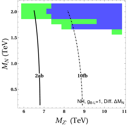
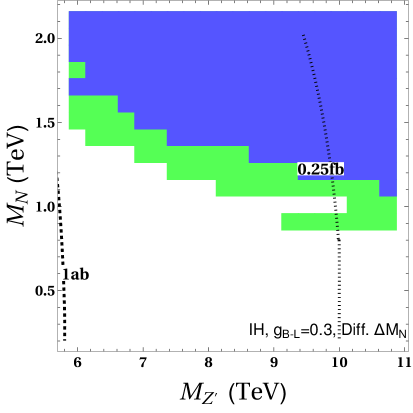
Figure 1: Prediction of the baryon asymmetry for $\eta_{B}\geq\eta_{B}^{\rm obs}$ in the $(M_{Z^{\prime}},M_{N})$ plane for a fixed $g_{B-L}=1\,(0.3)$ for NH (IH) in the $U(1)_{B-L}$ case. The green region indicates optimum RHN mass splitting ($\Delta M_{N,\text{opt}}$, see Eq. (3.7), and blue region indicates $\Delta M_{N}=10\,\Delta M_{N,\text{opt}}$. The contours show $\sigma_{\mathrm{prod}}$ (in ab/fb) at the $\sqrt{s}=14$ TeV LHC (solid/dashed) and at $\sqrt{s}=100$ TeV future collider (dot-dashed, dotted). Note : Blue region lies completely inside the green region.

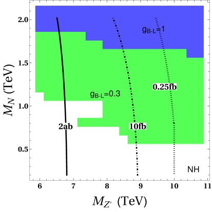
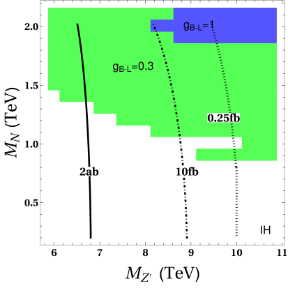
Figure 2: Prediction of the baryon asymmetry for $\eta_{B}\geq\eta_{B}^{\rm obs}$ shown in green (blue) region in the $(M_{Z^{\prime}},M_{N})$ plane for $g_{B-L}=0.3\,(1)$ for both NH and IH in $U(1)_{B-L}$ case. The contours show $\sigma_{\mathrm{prod}}$ (in ab/fb) at the $\sqrt{s}=14$ TeV LHC ($g_{B-L}=1$, solid) and at $\sqrt{s}=100$ TeV future collider ($g_{B-L}=0.3$, dashed) and ($g_{B-L}=1$, dot-dashed). Note : Blue region lies completely inside the green region.

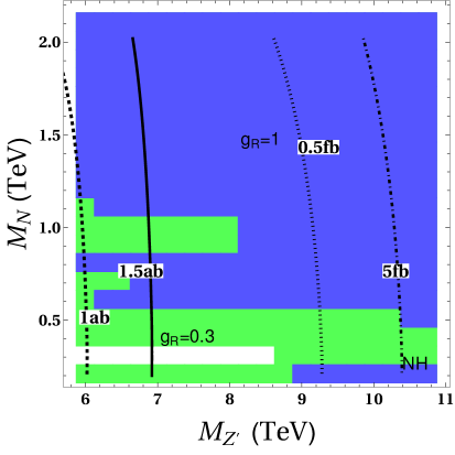
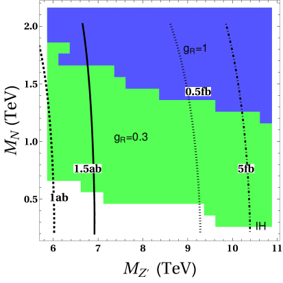
Figure 3: Prediction of the baryon asymmetry for $\eta_{B}\geq\eta_{B}^{\rm obs}$ shown in green (blue) region in the $(M_{Z^{\prime}},M_{N})$ plane for $g_{R}=0.3\,(1)$ for both NH and IH in $U(1)_{R}$ case. The contours show $\sigma_{\mathrm{prod}}$ (in ab/fb) at the $\sqrt{s}=14$ TeV LHC ($g_{R}=1$, solid), ($g_{R}=0.3$, dotted) and at $\sqrt{s}=100$ TeV future collider ($g_{R}=0.3$, dashed) and ($g_{R}=1$, dot-dashed). Note : Blue region lies completely inside the green region.

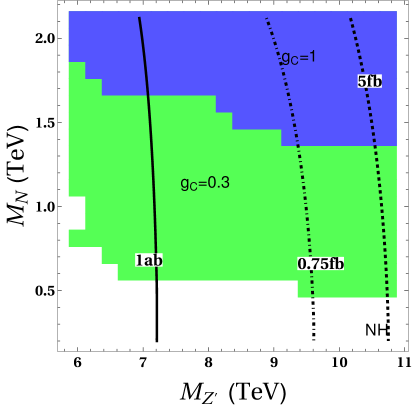
Figure 4: Prediction of the baryon asymmetry for $\eta_{B}\geq\eta_{B}^{\rm obs}$ shown in green (blue) region in the $(M_{Z^{\prime}},M_{N})$ plane for $g_{C}=0.3\,(1)$ for both NH and IH in $U(1)_{C}$ case. The contours show $\sigma_{\mathrm{prod}}$ (in ab/fb) at the $\sqrt{s}=14$ TeV LHC ($g_{C}=1$, solid) and at $\sqrt{s}=100$ TeV future collider ($g_{C}=0.3$, dashed) and ($g_{C}=1$, dot-dashed). Note : Blue region lies completely inside the green region.

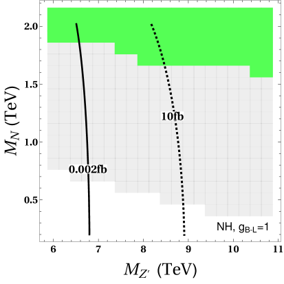
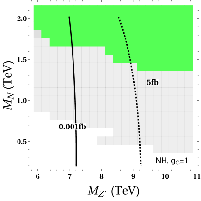
Figure 5: Baryon asymmetry production in flavored case (unflavored) for $\eta_{B}\geq\eta_{B}^{\rm obs}$ shown in green (grey) region in the $(M_{Z^{\prime}},M_{N})$ plane for NH and different $g_{X}=1$, where $X={(B-L,R,C)}$. The contours show $\sigma_{\mathrm{prod}}$ (in ab/fb) at the $\sqrt{s}=14$ TeV LHC (solid) and at $\sqrt{s}=100$ TeV future collider (dashed).

4 Results and Discussion

In this section, we compute the baryon asymmetry production in three scenarios with different $U(1)_{X}$ charges (described in Sec. 2), with the flavored Boltzmann transport formalism as described in previous section [18]. Firstly, we show the effect of mass-splitting on the predicted baryon asymmetry in the $U(1)_{B-L}$ case as a function of $(M_{Z^{\prime}},M_{N})$ for $g_{B-L}=1\,(0.3)$ for NH (IH) scenario. For these chosen values of the gauge-couplings, we choose to restrict $M_{Z^{\prime}}\geq 6$ TeV, to be consistent with the dilepton bounds from LEP-II [38]. The colored regions indicate the parameter space for $\eta_{B}\geq\eta_{B}^{\rm obs}$. The green region indicates optimum RHN mass splitting $\Delta M_{N,\text{opt}}$ and blue region indicates $\Delta M_{N}=10\,\Delta M_{N,\text{opt}}$. We clearly find that setting the $\Delta M_{N}$ to the optimum value gives the maximum parameter space consistent with the condition $\eta_{B}\geq\eta_{B}^{\rm obs}$. On increasing the $\Delta M_{N}$ by a factor of 10, we notice the parameter space reduces while still being a subset of the maximum parameter space allowed for optimal $\Delta M_{N}$. This is a general feature of the baryon asymmetry production for all $U(1)_{X}$ charges. Hence, we will hereafter set $\Delta M_{N}$ to the optimum value in all cases. Furthermore, we also include the collider sensitivity of the relevant parameter space in $(M_{Z^{\prime}},M_{N})$ plane. The contours show $\sigma_{\mathrm{prod}}$ (in ab/fb) at the $\sqrt{s}=14$ TeV LHC (solid/dashed) and at $\sqrt{s}=100$ TeV future collider (dot-dashed, dotted).

We now plot the predicted baryon asymmetry $\eta_{B}$ in the $(M_{Z^{\prime}},M_{N})$ plane for a fixed $g_{X}=(0.3,1)$ for both NH and IH in the $U(1)_{X},\,{X=(B\text{-}L,R,C)}$, shown in Figs. 2,3 and 4 for optimal $\Delta M_{N}$. For $U(1)_{B\text{-}L}$ in Fig. 2, successful leptogenesis is possible for $M_{N}>0.5(0.8)$ TeV for NH(IH) and $g_{B-L}=0.3$. Upon increasing the gauge coupling $g_{B-L}=1$, the parameter space shrinks due to increased washout effects and dilution. In this case, successful leptogenesis is only possible for $M_{N}>1.5(1.8)$ TeV for NH(IH), with $\sigma_{\mathrm{prod}}^{\text{NH}}=2$ ab at LHC and $\sigma_{\mathrm{prod}}^{\text{IH}}=10$ fb at future collider.

For $U(1)_{R}$ in Fig. 3, it can be seen that successful leptogenesis is possible for $M_{N}$ as low as $0.2$ TeV for both NH and IH if $g_{R}=0.3$, while for $g_{R}=1$, $M_{N}>0.2(1.2)$ TeV for NH(IH) is required. For all these cases, $\sigma_{\mathrm{prod}}$ at LHC reaches $\sim 1$-$1.5$ ab. Similarly for $U(1)_{C}$ in Fig. 4, successful leptogenesis is possible for $M_{N}>0.4(0.6)$ TeV for NH(IH) and $g_{C}=0.3$, while for $g_{C}=1$, $M_{N}>1.3(1.6)$ TeV for NH(IH) is required. The $\sigma_{\mathrm{prod}}$ reach at LHC for NH and IH for $g_{C}=1$ is around $\sim 1$ ab.

In addition to studying the flavored case, we also compare our results with the unflavored regime for all three $U(1)_{X}$ scenarios as shown in Fig. 5. In this figure, we plot the prediction for the baryon asymmetry production in the flavored case (shown in red) and unflavored case (shown in grey) in the $(M_{Z^{\prime}},M_{N})$ plane. We have chosen to set the respective gauge coupling in each case to be unity and with ordering set to NH. It can be clearly seen that in all cases, the unflavored treatment usually overestimates the parameter space for required baryon asymmetry. For eg., successful leptogenesis in $U(1)_{B\text{-}L}$ for unflavored case is possible for $M_{N}>0.3$ TeV, while in the proper treatment involving the flavored transport equations, $M_{N}>1.5$ TeV is required. Hence, flavor effects play an important role in determination of $\eta_{B}$ generated through resonant leptogenesis [29].

5 Conclusion

We have studied the generation of baryon asymmetry through the resonant leptogenesis for the $U(1)_{X}$ extension of the SM. We numerically solve the flavored Boltzmann transport equations to calculate the total baryon asymmetry generated. After maximizing the $\eta_{B}$ for given $M_{N}$ and $M_{Z^{\prime}}$, we show that the three different cases considered in this work can naturally explain the observed baryon asymmetry of the Universe in the large portion of the available parameter space. We find that the $U(1)_{C}$ case offers successful leptogenesis in a larger portion of the parameter space as compared to $U(1)_{B\text{-}L}$ and $U(1)_{R}$. We also perform a comparative study between the flavored and unflavored leptogenesis, showcasing the impact and importance of the flavor effects at play. Finally, we have also studied the collider prospects for all these different scenarios. We find that although HL-LHC might not be able to probe all the relevant parameter space, $\sqrt{s}=100$ TeV future collider can access these regions, thereby offering an opportunity to test resonant leptogenesis in the $U(1)_{X}$ model.

Appendix A Appendix

In this section, we provide the reduced cross sections used in this work for calculating the $\eta_{B}$ using flavored Boltzmaan transport equations. The form of $\hat{\sigma}=\frac{8\sigma}{s}[(p_{\text{in}}.p_{\text{out}})^{2}-m_{f}^{4}]$ where $\sigma$ is the total cross section in center of mass frame for the processes participating in the resonant leptogenesis, $p_{\text{in}}$ and $p_{\text{out}}$ are the momenta of incoming and outgoing state particles. The reduced cross sections involving Higgs $(h)$ have been obtained following [43].

• Scalar $(h)$ mediated $\ell N^{i}\to tq$ process in $s$-channel

  $$\hat{\sigma}(N^{i}\ell\leftrightarrow tq)=\frac{3\pi\alpha^{2}m_{t}}{M_{W}^{4}\sin\theta_{W}^{4}}(M_{D}^{\dagger}M_{D})_{ij}\Bigg{(}1-\frac{m_{N_{i}}^{2}}{s}\Bigg{)}^{2}$$ (A.1)

  Scalar $(h)$ mediated $N^{i}t\to\ell q$ process in $t$-channel

  $$\hat{\sigma}(N^{j}t\to\ell q)=\frac{3\pi\alpha^{2}m_{t}}{M_{W}^{4}\sin\theta_{W}^{4}}(M_{D}^{\dagger}M_{D})_{ij}\Bigg{[}1-\frac{m_{N_{i}}^{2}}{s}+\frac{m_{N_{i}}^{2}}{s}\log\Bigg{(}1+\frac{s-m_{N_{i}}^{2}}{m_{h}^{2}}\Bigg{)}\Bigg{]}$$ (A.2)

  where $\alpha=\frac{e^{2}}{4\pi}$.

• $\ell h\to\ell h$ process mediated by $N$ in the $s$-channel and $t$- channel

  $$\hat{\sigma}(\ell h\leftrightarrow\ell h) = \frac{2\alpha^{2}\pi~{}m_{N_{1}}^{2}}{\sin^{4}\theta_{W}M_{W}^{4}s}\Bigg{\{}\sum_{i=1}^{2}\frac{m_{N_{i}}^{2}}{m_{N_{1}}^{2}}(m_{D}^{\dagger}m_{D})_{ii}^{2}\Bigg{[}\frac{s}{m_{N_{i}}^{2}}+\frac{2s}{m_{N_{1}}^{2}\mathcal{D}_{i}}+$$ (A.3)

  $$\frac{s^{2}}{2m_{N_{1}}^{4}\mathcal{D}_{i}^{2}}-\Bigg{(}1+2\frac{s+m_{N_{i}}^{2}}{m_{N_{1}}^{2}\mathcal{D}_{i}}\Bigg{)}\log\Bigg{(}1+\frac{s}{m_{N_{j}}^{2}}\Bigg{)}\Bigg{]}+2\frac{m_{N_{2}}}{m_{N_{1}}}$$

  $$\mathcal{R}e\Bigg{[}(m_{D}^{\dagger}m_{D})_{12}^{2})\Bigg{]}\Bigg{[}\frac{s}{m_{N_{1}}^{2}\mathcal{D}_{1}}+\frac{s}{m_{N_{1}}^{2}\mathcal{D}_{2}}+\frac{s^{2}}{2m_{N_{1}}^{4}\mathcal{D}_{1}\mathcal{D}_{2}}-$$

  $$\frac{(s+m_{N_{1}}^{2})(s+m_{N_{1}}^{2}-2m_{N_{1}}^{2}m_{N_{2}}^{2})}{(m_{N_{1}}^{2}-m_{N_{2}}^{2})\mathcal{D}_{2}}\log\Bigg{(}\frac{s}{m_{N_{1}}^{2}}+1\Bigg{)}$$

  $$- \frac{(s+m_{N_{1}}^{2})(s+m_{N_{1}}^{2}-2m_{N_{1}}m_{N_{2}})}{(m_{N_{1}}-m_{N_{2}})m_{N_{1}}^{3}\mathcal{D}_{2}}\log\Big{(}\frac{s+m_{N_{1}}^{2}}{m_{N_{1}}^{2}}\Big{)}\Bigg{]}$$

  $$- \frac{(s+m_{N_{1}}m_{N_{2}})(s+m_{N_{1}}m_{N_{2}}-2m_{N_{1}}^{2})}{(m_{N_{1}}-m_{N_{2}})m_{N_{1}}^{3}\mathcal{D}_{2}}\log\Bigg{(}\frac{s+m_{N_{1}}m_{N_{2}}}{m_{N_{1}}m_{N_{2}}}\Bigg{)}\Bigg{\}}~{}~{}~{}$$

  where $\mathcal{D}_{i}=\frac{(s-m_{N_{j}}m_{N_{1}})^{2}+m_{N_{j}}m_{N_{1}}\Gamma_{ij}^{2}}{m_{N_{1}}^{2}(s-m_{N_{i}}m_{N_{1}})}$ is the off-shell part of the propagator.

• $\ell\ell\leftrightarrow hh$ process mediated by $N$ in the $t$- channel

  $$\hat{\sigma}(\ell\ell\leftrightarrow hh) = \frac{2\pi\alpha^{2}}{M_{W}^{4}\sin\theta_{W}^{4}}\Bigg{\{}\sum_{i=1}^{2}\frac{m_{N_{i}}}{m_{N_{1}}}(m_{D}^{\dagger}m_{D})_{ii}^{2}\Bigg{[}\frac{m_{N_{1}}s}{2m_{N_{j}}(s+m_{N_{j}}m_{N_{1}})}$$ (A.4)

  $$+ \frac{m_{N_{1}}^{2}}{(s+2m_{N_{j}}m_{N_{1}})}\log\Bigg{(}\frac{s+m_{N_{1}}m_{N_{j}}}{m_{N_{1}}m_{N_{j}}}\Bigg{)}\Bigg{]}+\mathcal{R}e\Bigg{[}(m_{D}^{\dagger}m_{D})_{12}^{2}\Bigg{]}$$

  $$\frac{\sqrt{m_{N_{1}}m_{N_{2}}}m_{N_{1}}^{2}}{(m_{N_{1}}-m_{N_{2}})(s+m_{N_{1}}+m_{N_{1}}m_{N_{2}})}\Bigg{[}\frac{s+2m_{N_{1}}^{2}}{m_{N_{1}}^{2}}\log\Bigg{(}\frac{s}{m_{N_{1}}m_{N_{2}}}+1\Bigg{)}$$

  $$- \frac{s+2m_{N_{2}}m_{N_{1}}}{m_{N_{1}}^{2}}\log\Bigg{(}\frac{(s+m_{N_{1}}^{2})}{m_{N_{1}}^{2}}\Bigg{)}\Bigg{]}\Bigg{\}}.$$

• Pair production of $N$ from different initial SM charged fermions:

  $$\hat{\sigma}(f\bar{f}\leftrightarrow N_{i}N_{i})=\frac{g_{X}^{4}x_{\Phi}^{2}s^{2}}{12\pi}\Bigg{[}\frac{(1-\frac{4m_{N_{i}}^{2}}{s})^{\frac{3}{2}}}{(s-{m_{Z}^{\prime}}^{2})^{2}+{\Gamma_{Z}^{\prime}}^{2}{m_{Z}^{\prime}}^{2}}\Bigg{]}(C_{A}^{2}+C_{V}^{2})$$ (A.5)

  where the vector and axial-vector couplings are given in Tab. 2 considering $x_{\Phi}=1$. This cross section should be averaged over the color factor for quarks.

  Type of fermion	vector coupling $(C_{V})$	axial vector coupling $(C_{A})$
  	$\frac{q_{f_{L}}+q_{f_{R}}}{2}$	$\frac{q_{f_{L}}-q_{f_{R}}}{2}$
  charged lepton $(\ell)$	$-\frac{3}{4}x_{H}-1$	$\frac{1}{4}x_{H}$
  up-type quarks $(q_{u})$	$\frac{5}{12}x_{H}+\frac{1}{3}$	$-\frac{1}{4}x_{H}$
  down-type quarks $(q_{d})$	$-\frac{1}{12}x_{H}+\frac{1}{3}$	$-\frac{1}{4}x_{H}$

  Table 2: Vector and axial-vector couplings of different SM charged fermions with $Z^{\prime}$ where the axial vector couplings vanish for $x_{H}=0$ case.

• For $i\neq j$, RHN pair production cross section is

  $$\sigma(N_{i}N_{i}\leftrightarrow N_{j}N_{j}) = \frac{g_{X}^{4}x_{\Phi}^{4}\sqrt{(s-4m_{N_{j}}^{2})(s-4m_{N_{i}}^{2})}}{72\pi\{(s-m_{Z^{\prime}}^{2})^{2}+\Gamma_{Z^{\prime}}^{2}m_{Z^{\prime}}^{2}\}}$$ (A.6)

  $$\Bigg{[}(s-4m_{N_{j}}^{2})(s-4m_{N_{i}}^{2})+12\frac{m_{N_{i}}^{2}m_{N_{j}}^{2}}{m_{Z^{\prime}}^{4}}(s-m_{Z^{\prime}})^{2}\Bigg{]}$$

  For the other case,

  $$\hat{\sigma}(N_{i}N_{i}\leftrightarrow N_{i}N_{i}) = \frac{g_{X}^{4}x_{\Phi}^{4}}{128\pi}\Bigg{[}\frac{(s-4m_{N_{i}}^{2})^{3}}{3s((s-m_{Z^{\prime}}^{2})^{2}+m_{Z^{\prime}}^{2}\Gamma_{Z^{\prime}}^{2})}+\frac{(s-4m_{N_{i}}^{2})}{sm_{Z^{\prime}}^{4}(s-4m_{N_{i}}^{2}+m_{Z^{\prime}}^{2})}\Big{\{}m_{Z^{\prime}}^{2}(s-4m_{N_{i}}^{2})^{2}+$$ (A.7)

  $$2(m_{Z^{\prime}}^{2}-2m_{N_{i}}^{2})^{3}+s(8m_{N_{i}}^{4}+3m_{Z^{\prime}}^{4})-4m_{N_{i}}^{2}(m_{Z^{\prime}}^{4}+4m_{N_{i}}^{4}+m_{Z^{\prime}}^{2}m_{N_{i}}^{2})\Big{\}}+$$

  $$+\Big{\{}\frac{(3m_{Z^{\prime}}^{2}-4m_{N_{i}}^{2})(s-4m_{N_{i}}^{2})^{2}+m_{Z^{\prime}}^{4}(3s-20m_{N_{i}}^{2})+2m_{Z^{\prime}}^{2}(m_{Z^{\prime}}^{4}+8m_{N_{i}}^{4})}{sm_{Z^{\prime}}^{2}(s-4m_{N_{i}}^{2}+2m_{Z^{\prime}}^{2})}\Big{\}}$$

  $$\log\Big{(}\frac{m_{Z^{\prime}}^{2}}{s-4m_{N_{i}}^{2}+m_{Z^{\prime}}^{2}}\Big{)}\Bigg{]}~{}~{}~{}~{}~{}$$

• Pair production of $N$ from Higgs $(h)$ in the $s$-channel:

  $$\hat{\sigma}(hh\leftrightarrow N_{i}N_{i})=\frac{{g_{X}^{4}}x_{\Phi}^{4}}{12\pi}\frac{(x-4)^{\frac{3}{2}}(1-\frac{4{m_{\Phi}}^{2}}{xm_{N_{i}}^{2}})^{\frac{3}{2}}\sqrt{x}}{cy+(x-y)^{2}}$$ (A.8)

  where $x=\frac{s}{m_{N_{i}}^{2}}$, $y=\frac{m_{Z^{\prime}}^{2}}{m_{N_{i}}^{2}}$, $c=\frac{\Gamma_{Z^{\prime}}^{2}}{m_{N}^{2}}$ and $\Gamma_{Z^{\prime}}$ is the total decay width of $Z^{\prime}$. Reduced cross section for $\Phi$ pair production from RHN in $t-$channel and $u-$channel processes:

  $$\hat{\sigma}(N_{i}N_{i}\leftrightarrow hh)=\frac{Y_{N}^{4}}{8\pi}\Bigg{(}1-\frac{4m_{N_{i}}^{2}}{s}\Bigg{)}\Bigg{[}\frac{s-4m_{N_{i}}^{2}}{2m_{N_{i}}^{2}}+\Bigg{(}1-\frac{4m_{N_{i}}^{2}}{s}\Bigg{)}^{\frac{3}{2}}+\log\Bigg{(}\frac{s-\sqrt{s(s-4m_{N_{i}}^{2})}}{s+\sqrt{s(s-4m_{N_{i}}^{2})}}\Bigg{)}\Bigg{]}~{}~{}~{}~{}~{}$$ (A.9)

References

- [1] Particle Data Group collaboration, Review of Particle Physics, PTEP 2022 (2022) 083C01.
- [2] P. Minkowski, at a Rate of One Out of Muon Decays?, Phys. Lett. B 67 (1977) 421.
- [3] T. Yanagida, Horizontal gauge symmetry and masses of neutrinos, Conf. Proc. C 7902131 (1979) 95.
- [4] M. Gell-Mann, P. Ramond and R. Slansky, Complex Spinors and Unified Theories, Conf. Proc. C 790927 (1979) 315 [1306.4669].
- [5] R. N. Mohapatra and G. Senjanovic, Neutrino Mass and Spontaneous Parity Nonconservation, Phys. Rev. Lett. 44 (1980) 912.
- [6] S. L. Glashow, The Future of Elementary Particle Physics, NATO Sci. Ser. B 61 (1980) 687.
- [7] Planck collaboration, Planck 2018 results. VI. Cosmological parameters, Astron. Astrophys. 641 (2020) A6 [1807.06209].
- [8] M. Fukugita and T. Yanagida, Baryogenesis Without Grand Unification, Phys. Lett. B 174 (1986) 45.
- [9] V. A. Kuzmin, V. A. Rubakov and M. E. Shaposhnikov, On the Anomalous Electroweak Baryon Number Nonconservation in the Early Universe, Phys. Lett. B 155 (1985) 36.
- [10] S. Davidson and A. Ibarra, A Lower bound on the right-handed neutrino mass from leptogenesis, Phys. Lett. B 535 (2002) 25 [hep-ph/0202239].
- [11] W. Buchmuller, P. Di Bari and M. Plumacher, Cosmic microwave background, matter - antimatter asymmetry and neutrino masses, Nucl. Phys. B 643 (2002) 367 [hep-ph/0205349].
- [12] K. Moffat, S. Pascoli, S. T. Petcov, H. Schulz and J. Turner, Three-flavored nonresonant leptogenesis at intermediate scales, Phys. Rev. D 98 (2018) 015036 [1804.05066].
- [13] A. Pilaftsis and T. E. J. Underwood, Resonant leptogenesis, Nucl. Phys. B 692 (2004) 303 [hep-ph/0309342].
- [14] A. Pilaftsis, CP violation and baryogenesis due to heavy Majorana neutrinos, Phys. Rev. D 56 (1997) 5431 [hep-ph/9707235].
- [15] M. Drewes, B. Garbrecht, P. Hernandez, M. Kekic, J. Lopez-Pavon, J. Racker et al., ARS Leptogenesis, Int. J. Mod. Phys. A 33 (2018) 1842002 [1711.02862].
- [16] A. Pilaftsis and T. E. J. Underwood, Electroweak-scale resonant leptogenesis, Phys. Rev. D 72 (2005) 113001 [hep-ph/0506107].
- [17] F. F. Deppisch and A. Pilaftsis, Lepton Flavour Violation and theta(13) in Minimal Resonant Leptogenesis, Phys. Rev. D 83 (2011) 076007 [1012.1834].
- [18] P. S. B. Dev, P. Millington, A. Pilaftsis and D. Teresi, Flavour Covariant Transport Equations: an Application to Resonant Leptogenesis, Nucl. Phys. B 886 (2014) 569 [1404.1003].
- [19] P. S. B. Dev, M. Garny, J. Klaric, P. Millington and D. Teresi, Resonant enhancement in leptogenesis, Int. J. Mod. Phys. A 33 (2018) 1842003 [1711.02863].
- [20] T. Appelquist, B. A. Dobrescu and A. R. Hopper, Nonexotic Neutral Gauge Bosons, Phys. Rev. D 68 (2003) 035012 [hep-ph/0212073].
- [21] S. Iso, N. Okada and Y. Orikasa, Resonant Leptogenesis in the Minimal B-L Extended Standard Model at TeV, Phys. Rev. D 83 (2011) 093011 [1011.4769].
- [22] C. Coriano, L. Delle Rose and C. Marzo, Vacuum Stability in U(1)-Prime Extensions of the Standard Model with TeV Scale Right Handed Neutrinos, Phys. Lett. B 738 (2014) 13 [1407.8539].
- [23] S. Oda, N. Okada and D.-s. Takahashi, Classically conformal U(1)’ extended standard model and Higgs vacuum stability, Phys. Rev. D 92 (2015) 015026 [1504.06291].
- [24] A. Das, S. Oda, N. Okada and D.-s. Takahashi, Classically conformal U(1)’ extended standard model, electroweak vacuum stability, and LHC Run-2 bounds, Phys. Rev. D 93 (2016) 115038 [1605.01157].
- [25] A. Davidson, as the fourth color within an model, Phys. Rev. D 20 (1979) 776.
- [26] R. E. Marshak and R. N. Mohapatra, Quark - Lepton Symmetry and B-L as the U(1) Generator of the Electroweak Symmetry Group, Phys. Lett. B 91 (1980) 222.
- [27] W. Buchmuller, C. Greub and P. Minkowski, Neutrino masses, neutral vector bosons and the scale of B-L breaking, Phys. Lett. B 267 (1991) 395.
- [28] S. Blanchet, Z. Chacko, S. S. Granor and R. N. Mohapatra, Probing Resonant Leptogenesis at the LHC, Phys. Rev. D 82 (2010) 076008 [0904.2174].
- [29] P. S. B. Dev, P. Di Bari, B. Garbrecht, S. Lavignac, P. Millington and D. Teresi, Flavor effects in leptogenesis, Int. J. Mod. Phys. A 33 (2018) 1842001 [1711.02861].
- [30] J. A. Casas and A. Ibarra, Oscillating neutrinos and , Nucl. Phys. B 618 (2001) 171 [hep-ph/0103065].
- [31] L. Basso, A. Belyaev, S. Moretti and C. H. Shepherd-Themistocleous, Phenomenology of the minimal B-L extension of the Standard model: Z’ and neutrinos, Phys. Rev. D 80 (2009) 055030 [0812.4313].
- [32] P. Fileviez Perez, T. Han and T. Li, Testability of Type I Seesaw at the CERN LHC: Revealing the Existence of the B-L Symmetry, Phys. Rev. D 80 (2009) 073015 [0907.4186].
- [33] Z. Kang, P. Ko and J. Li, New Avenues to Heavy Right-handed Neutrinos with Pair Production at Hadronic Colliders, Phys. Rev. D 93 (2016) 075037 [1512.08373].
- [34] P. Cox, C. Han and T. T. Yanagida, LHC Search for Right-handed Neutrinos in Models, JHEP 01 (2018) 037 [1707.04532].
- [35] G. Chauhan and P. S. B. Dev, Interplay between resonant leptogenesis, neutrinoless double beta decay and collider signals in a model with flavor and CP symmetries, Nucl. Phys. B 986 (2023) 116058 [2112.09710].
- [36] B. Dutta, S. Ghosh and J. Kumar, A sub-GeV dark matter model, Phys. Rev. D 100 (2019) 075028 [1905.02692].
- [37] A. Das, N. Okada and D. Raut, Enhanced pair production of heavy Majorana neutrinos at the LHC, Phys. Rev. D 97 (2018) 115023 [1710.03377].
- [38] A. Das, P. S. B. Dev, Y. Hosotani and S. Mandal, Probing the minimal U(1)X model at future electron-positron colliders via fermion pair-production channels, Phys. Rev. D 105 (2022) 115030 [2104.10902].
- [39] M. Blennow, E. Fernández-Martínez, J. Hernández-García, J. López-Pavón, X. Marcano and D. Naredo-Tuero, Bounds on lepton non-unitarity and heavy neutrino mixing, JHEP 08 (2023) 030 [2306.01040].
- [40] P. S. B. Dev, P. Millington, A. Pilaftsis and D. Teresi, Kadanoff–Baym approach to flavour mixing and oscillations in resonant leptogenesis, Nucl. Phys. B 891 (2015) 128 [1410.6434].
- [41] J. Klarić, M. Shaposhnikov and I. Timiryasov, Uniting Low-Scale Leptogenesis Mechanisms, Phys. Rev. Lett. 127 (2021) 111802 [2008.13771].
- [42] A. Das and Y. Orikasa, Resonant leptogenesis in minimal extensions of the Standard Model, 2407.05644.
- [43] M. Plumacher, Baryogenesis and lepton number violation, Z. Phys. C 74 (1997) 549 [hep-ph/9604229].