Structure and Independence in Hyperbolic Uniform Disk Graphs

Abstract

We consider intersection graphs of disks of radius $r$ in the hyperbolic plane. Unlike the Euclidean setting, these graph classes are different for different values of $r$, where very small $r$ corresponds to an almost-Euclidean setting and $r\in\Omega(\log n)$ corresponds to a firmly hyperbolic setting. We observe that larger values of $r$ create simpler graph classes, at least in terms of separators and the computational complexity of the Independent Set problem.

First, we show that intersection graphs of disks of radius $r$ in the hyperbolic plane can be separated with $\mathcal{O}((1+1/r)\log n)$ cliques in a balanced manner. Our second structural insight concerns Delaunay complexes in the hyperbolic plane and may be of independent interest. We show that for any set $S$ of $n$ points with pairwise distance at least $2r$ in the hyperbolic plane the corresponding Delaunay complex has outerplanarity $1+\mathcal{O}(\frac{\log n}{r})$, which implies a similar bound on the balanced separators and treewidth of such Delaunay complexes.

Using this outerplanarity (and treewidth) bound we prove that Independent Set can be solved in $n^{\mathcal{O}(1+\frac{\log n}{r})}$ time. The algorithm is based on dynamic programming on some unknown sphere cut decomposition that is based on the solution. The resulting algorithm is a far-reaching generalization of a result of Kisfaludi-Bak (SODA 2020), and it is tight under the Exponential Time Hypothesis. In particular, Independent Set is polynomial-time solvable in the firmly hyperbolic setting of $r\in\Omega(\log n)$. Finally, in the case when the disks have ply (depth) at most $\ell$, we give a PTAS for Maximum Independent Set that has only quasi-polynomial dependence on $1/\varepsilon$ and $\ell$. Our PTAS is a further generalization of our exact algorithm.

1 Introduction

Given a set of disks in the plane, one can assign to them a geometric intersection graph whose vertices are the disks, and edges are added between pairs of intersecting disks. The study of intersection graphs is usually motivated by physically realized networks: such networks require spatial proximity between nodes for successful connections, and the simplest model allows for connections within a distance $2$, which is equivalent to the intersection graph induced by disks of radius $1$ centered at the nodes. Such graphs are usually called unit disk graphs.

Unit disk graphs have received a lot of attention in the theoretical computer science literature. Their intriguing structural properties yield profound mathematical insights and facilitate the development of efficient algorithms. Historically, unit disk graphs have been studied in the Euclidean plane, where they are well motivated due to their relevance for, e.g., sensor networks. The relevance of unit disk graphs in the hyperbolic plane is less obvious. However, originating in the network science community, it has been observed [31] that the intersection graph of randomly sampled disks of equal radius $r$ yields graphs that resemble complex real-world networks in regards to important properties. They are, e.g., heterogeneous with a degree distribution following a power law [21], have high clustering coefficient [21], and exhibit the small-world property [19, 40].

Besides numerous structural results, these hyperbolic random graphs also allow for the design of more efficient algorithms [10, 7, 6, 8]. However, all these results rely on the fact that the disks are chosen randomly. So far, there is only little research on hyperbolic uniform disk graphs from a deterministic, more graph-theoretic perspective. It is important to note that for the intersection graphs of radius-$r$ disks the resulting graph classes are different for different values of $r$. Moreover, it is natural to allow for the radius $r$ to be a (monotone) function of the number of vertices. Unlike the Euclidean setting where a simple scaling shows that the choice of “unit” does not matter, it is a very important parameter in the hyperbolic setting.

For those unfamiliar with hyperbolic geometry there is a way to conceptually understand these graphs in a Euclidean setting as follows. One can think of a hyperbolic disk graph of radius $r$ disks as a Euclidean disk graph where the radius of a disk of center $p$ is set to $f_{r}(\operatorname{\mathrm{dist}}(o,p))$, where $f_{r}$ is decreasing very quickly at a rate set by $r$, and $\operatorname{\mathrm{dist}}(o,p)$ is the distance of the origin and the disk center $p$. In particular, as $r$ goes to $0$, the rate of decrease is negligible, and we get almost Euclidean unit disk graphs, while large $r$ corresponds to a very different graph class. See Figure 1 for an illustration.

Now hyperbolic disk graphs of uniform (that is, equal) radius $1/n^{3}$ and uniform radius $100\log n$ are incomparable: the former class contains all $k\times k$ grid graphs, but does not contain stars of size $s\geq 8$, while the latter contains all star graphs but does not contain any $k\times k$ grid of size $k\geq 3$, see Figure 1. We call the regime $r\leq 1/\sqrt{n}$ almost Euclidean, while $r\in\Omega(\log n)$ is called firmly hyperbolic.

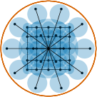
(a) Smaller $r$ allows for larger grids.

(b) Only small stars for small $r$.

(c) Larger $r$ allows for larger stars.

Figure 1: Realizing a grid is only possible for small radii, while large stars are only possible in the firmly hyperbolic setting of $r\in\Omega(\log n)$.

The primary goal of our paper is to explore the following:

How does the structure of hyperbolic uniform disk graphs depend on the radius $r=r(n)$?

The case of constant radius has been studied by Kisfaludi-Bak [28], and a case of radius roughly $\log n$ (with some other constraints) has been studied by Bläsius et al. [9] in the context of strongly hyperbolic uniform disk graphs. The above mentioned hyperbolic random graphs are randomly sampled strongly hyperbolic uniform disk graphs. Apart from these particular choices of the radius we have very limited understanding about the structure of hyperbolic uniform disk graphs of other radii. The radius’ impact on problem complexity was studied in the context of the traveling salesman problem in the hyperbolic plane [27], where the problem’s complexity decreases as one increases the minimum pairwise distance $r$ among input points. In this paper, we show that the structure of hyperbolic uniform disk graphs behaves similarly: their structure becomes easier for larger values of $r$, and Independent Set can be solved faster for larger $r$.

Let $\mathrm{HUDG}(r(n))$ denote the set of intersection graphs where each $n$-vertex graph can be realized as the intersection graph of disks of uniform (equal) radius $r(n)$ in the hyperbolic plane of Gaussian curvature $-1$. We denote by $\mathrm{HUDG}$ the union of these classes for all $r$, that is, $\mathrm{HUDG}=\bigcup_{r>0}\mathrm{HUDG}(r)$. Let $\mathrm{UDG}$ denote the class of unit disk graphs in the Euclidean plane. Bläsius et al. have shown that $\mathrm{UDG}\subset\mathrm{HUDG}$ [9]. When a graph is given without the geometric realization, it is NP-hard (even $\exists\mathbb{R}$-complete) to decide if the graph is a $\mathrm{UDG}$ [38] or $\mathrm{HUDG}$ [5]; for this reason, we will assume throughout this article that the input intersection graphs of our algorithms are given by specifying their geometric realization. In the hyperbolic setting, one can specify the disk centers using a so-called model of the hyperbolic plane, which is simply an embedding of the hyperbolic plane into some specific part of the Euclidean plane, e.g., inside the Euclidean unit disk. See our preliminaries for brief introduction to Euclidean models of the hyperbolic plane.

From the perspective of graph algorithms, unit disk graphs in the Euclidean plane have been serving an important role as a graph class that is not comparable but similar to planar graphs. The circle packing theorem [30] states that every planar graph can be realized as an intersection graph of disks (of arbitrary radii), thus disk graphs serve as a common generalization of planar and unit disk graphs. Using conformal hyperbolic models, one can observe that hyperbolic disks appear as Euclidean disks in the model, which means that all $\mathrm{HUDG}$s are realized as Euclidean disk graphs. Denoting Euclidean disk graphs with $\mathrm{DG}$, we thus have $\mathrm{UDG}\subseteq\mathrm{HUDG}\subseteq\mathrm{DG}$.

A key structural tool in the study of both planar and (unit) disk graphs has been separator theorems. By a result of Lipton and Tarjan[32], any $n$-vertex planar graph can be partitioned into three vertex sets, $A,B$ and the separator $S$, such that no edges go between $A$ and $B$, the separator set $S$ has size $\mathcal{O}(\sqrt{n})$, and $\max\{|A|,|B|\}\leq\frac{2}{3}n$. Separator theorems are closely related to the treewidth of graphs [11], for example, the above separator implies a treewidth bound of $O(\sqrt{n})$ on planar graphs.

For (unit) disk graphs, similar separators and treewidth bounds are not possible because one can represent cliques of arbitrary size. There have been at least three different approaches to deal with large cliques. The first option is to bound the cliques in some way. One can for example obtain separators for a set of disks of bounded ply, i.e., assuming that each point of the ambient space is included in at most $\ell$ disks. There are several separators for disks (and even balls in higher dimensions) that involve ply. The strongest and most general among these is by Miller et al. [39]. The second way to deal with large cliques is to use so-called clique-based separators [3, 4], where the separator is decomposed into cliques, and the cliques are sometimes assigned some small weight depending on their size. In the hyperbolic setting, Kisfaludi-Bak [28] showed that for any constant $c$, the graph class $\mathrm{HUDG}(c)$ admits a balanced separator consisting of $\mathcal{O}(\log n)$ cliques. The same paper shows that $\mathrm{HUDG}(c)$ also has clique-based separators of weight $\mathcal{O}(\log^{2}n)$, and extends these techniques to balls of constant radius in higher-dimensional hyperbolic spaces, along with much of the machinery of [3]. The third option is to use random disk positions to disperse large cliques with high probability. Bläsius, Friedrich and Krohmer [10] gave high-probability bounds on separators and treewidth for certain radius regimes in hyperbolic random graphs.

The above separators and treewidth can be used to obtain fast divide-and-conquer or dynamic programming algorithms [33, 3]. In the Independent Set problem, the goal is to decide if there are $k$ pairwise non-adjacent vertices in the graph. In general graphs the best known algorithms run in $2^{\mathcal{O}(n)}$ or $n^{\mathcal{O}(k)}$ time, and these running times are optimal under the Exponential Time Hypothesis (ETH) [15] (see [25] for the definition of ETH). In planar and disk graphs however the separators allow algorithms with running time $2^{\mathcal{O}(\sqrt{n})}$ or $n^{\mathcal{O}(\sqrt{k})}$ [15, 37]. Moreover, the separator implies that planar graphs have treewidth⁵ $\mathcal{O}(\sqrt{n})$ and unit disk graphs have so-called $\mathcal{P}$-flattened treewidth $\mathcal{O}(\sqrt{n})$ for some clique-partition $\mathcal{P}$. As a consequence, one can adapt treewidth-based algorithms [15] to these graph classes. In the hyperbolic setting, the ($\mathcal{P}$-flattened) treewidth bounds yield an $n^{\mathcal{O}(\log n)}$ quasi-polynomial algorithm for Independent Set and many other problems on graphs in $\mathrm{HUDG}(c)$ for any constant $c$ which is matched by a lower bound under ETH [28] in case of Independent Set.

When approximating Independent Set, the main algorithmic tool in planar graphs is Baker’s shifting technique [2] which gives a $(1-\varepsilon)$-approximate independent set in $2^{\mathcal{O}(1/\varepsilon)}n$ time. A conceptually easier grid shifting was discovered for unit disks by Hochbaum and Maas [24], which was later (implicitly) improved by Agarwal, van Kreveld, and Suri [1]. This line of research culminated in the algorithm of Chan [14] with a running time of $n^{\mathcal{O}(1/\varepsilon)}$ for disks, which also can be generalized for balls in higher dimensions. Baker’s algorithm and Chan’s algorithm (even for unit disks) are optimal under standard complexity assumptions [35]. To the best of our knowledge, there are no published approximation algorithms for $\mathrm{HUDG}(r(n))$ or $\mathrm{HUDG}$ other than what is already implied from the algorithms on disk graphs. However, for hyperbolic random graphs, there is an $\mathcal{O}(m\log n)$ algorithm that yields a $1-o(1)$-approximation for Independent Set asymptotically almost surely [8].

An interesting setting where the treewidth of planar graphs has been used for intersection graphs is that of covering and packing problems in the work of Har-Peled and later Marx and Pilipczuk [23, 37]. For the Independent Set problem on unit disk graphs, they consider the Voronoi diagram of the disk centers of a maximum independent set of size $k$. For a set of points (often called sites) $S$ the Voronoi diagram is a planar subdivision (a planar graph) that partitions the plane according to the closest site of $S$, that is, the cell of a site $s\in S$ consists of those points whose nearest neighbor from $S$ is $s$. As the Voronoi diagram is a planar graph on $\mathcal{O}(k)$ vertices, it has a balanced separator of size $\mathcal{O}(\sqrt{k})$. Although this Voronoi diagram is based on the solution, and thus unknown from the algorithmic perspective, the idea of Marx and Pilipczuk is that one can enumerate all possible separators of the Voronoi diagram in $n^{\mathcal{O}(\sqrt{k})}$ time, and one of these separators can then be used to separate the (still unknown) solution in a balanced manner. A similar “separator guessing” technique has been used elsewhere in approximation and parameterized algorithms [36, 13].

Our contribution.

Our first structural result is a balanced clique-based separator theorem presented in Section 3. We note that all of our results in hyperbolic uniform disk graphs assume that the graph is given via some geometric representation, i.e., with the Euclidean coordinates of its disk centers in some Euclidean model of the hyperbolic plane.

Theorem 1.

Let $G$ be a hyperbolic uniform disk graph with radius $r$. Then $G$ has a separator $S$ that can be covered with $\mathcal{O}\big{(}\log n\cdot\big{(}1+\frac{1}{r}\big{)}\big{)}$ cliques, such that all connected components of $G-S$ have at most $\frac{2}{3}n$ vertices. The separator can be computed in $\mathcal{O}(n\log n)$ time.

Our separator is in fact a carefully chosen line; the proof bounds the number of cliques intersecting the separator via decomposing some neighborhood of the chosen line into a small collection of small diameter regions. Notice that the theorem guarantees a separator with $\mathcal{O}(\log n)$ cliques in the hyperbolic setting, and deteriorates linearly as a function of $1/r$. In the almost-Euclidean setting of $r=1/\sqrt{n}$ the separator has $\mathcal{O}(\sqrt{n}\log n)$ cliques, which almost matches the $\mathcal{O}(\sqrt{n})$ clique separator for unit disk graphs [3]. This is also a direct generalization of the $2$-dimensional separator of Kisfaludi-Bak [28] from $r\in\Theta(1)$ to general radii.

Moreover, in Section 7 we observe that the techniques of [3, 28] can be utilized as the above separator implies $\mathcal{P}$-flattened treewidth $\mathcal{O}\left(\log^{2}n\left(1+\frac{1}{r}\right)\right)$ for any natural clique partition $\mathcal{P}$.

[] Let $G$ be a hyperbolic uniform disk graph with radius $r$. Then a maximum independent set of $G$ can be computed in $n^{\mathcal{O}((1+1/r)\log^{2}n)}$ time.

Thus, a quasi-polynomial $n^{\mathcal{O}(\log^{2}n)}$ algorithm is possible for all $r\in\Omega(1)$. If $r\leq 1$ — or even $r\in\mathcal{O}(1)$ — then for any $G\in\mathrm{HUDG}(r)$ the neighborhood of a disk can be covered by a constant number of cliques of $G$ (see also [28] for the case $r\in\Theta(1)$). Together with our separator in Theorem 1, the machinery of [3, 28] now yields the following result.

[] Let $G$ be a hyperbolic uniform disk graph with radius $r\in\mathcal{O}(1)$. Then Dominating Set, Vertex Cover, Feedback Vertex Set, Connected Dominating Set, Connected Vertex Cover, Connected Feedback Vertex Set can be solved in $n^{\mathcal{O}((1/r)\log n)}$ time, and $q$-Coloring for $q\in\mathcal{O}(1)$, Hamiltonian Path and Hamiltonian Cycle can be solved in $n^{\mathcal{O}(1/r)}$ time.

While the above separator is already powerful and can be used as a basis for quasi-polynomial divide-and-conquer algorithms, the separator size stops improving when increasing the radius $r$ beyond a constant. Nonetheless, a more powerful result is possible for super-constant radius $r$, which requires a different type of separator. Rather than separating hyperbolic uniform disk graphs, our second structural result is about separating the Delaunay complex, which is the dual of the Voronoi diagram, of a set of sites with pairwise distance at least $2r$. Note that in some graph $G\in\mathrm{HUDG}(r)$, the disk centers corresponding to an independent set will have pairwise distance more than $2r$, which is what motivated us to study such point sets.

A plane graph (a planar graph with a fixed planar embedding) is called outerplanar or $1$-outerplanar if all of its vertices are on the unbounded face. A plane graph is called $k$-outerplanar if deleting the vertices of the unbounded face (and all edges incident to them) yields a $(k-1)$-outerplanar graph. Our result concerns the outerplanarity of a Delaunay complex. We prove the following tight result on the outerplanarity of the Delaunay complex $\mathcal{D}(S)$ of such a site set $S$. We believe that this result presented in Section 4 may be of independent interest.

Theorem 2.

Let $S$ be a set of $n$ sites (points) in $\mathbb{H}^{2}$ with pairwise distance at least $2r$. Then the Delaunay complex $\mathcal{D}(S)$ is $1+\mathcal{O}\big{(}\frac{\log n}{r}\big{)}$-outerplanar.

In plane graphs, the treewidth, the outerplanarity, and the dual graph’s treewidth and outerplanarity are all within a constant multiplicative factor of each other [11, 12]. Consequently, we get the bound $\mathcal{O}\big{(}1+\frac{\log n}{r}\big{)}$ for the treewidth and outerplanarity of the Voronoi diagram and Delaunay complex of such point sets. Note that this implies constant outerplanarity for the firmly hyperbolic setting of $r\in\Omega(\log n)$.

Figure 2: A Euclidean Delaunay complex of $n$ points with outerplanarity $n/3$.

In particular, the theorem shows that for some constant $c$ and $r>c\log n$ the Delaunay complex is outerplanar. We recover the outerplanarity bound of [28] for $r=\Theta(1)$, and get a sublinear outerplanarity bound ($\mathcal{O}(\sqrt{n}\log n)$) even in the almost-Euclidean setting of $r=1/\sqrt{n}$. This is surprising in light of the fact that Delaunay-triangulations can have outerplanarity $\Omega(n)$ in the Euclidean setting, as demonstrated by the set of sites in Figure 2. Notice however that the construction requires a point set where the ratio of the maximum and minimum distance among the points is $\Omega(n)$; mimicking this construction in $\mathbb{H}^{2}$ with a point set of minimum distance $r=1/\sqrt{n}$ is not possible as at distance $n\cdot r=\sqrt{n}$ the hyperbolic distortion is very significant compared to the Euclidean setting.

Using the outerplanarity bound, we are able to give the following algorithm for Independent Set in Section 5.

Theorem 3.

Let $G$ be a hyperbolic uniform disk graph with radius $r$ and let $k\geq 0$. Then we can decide if there is an independent set of size $k$ in $G$ in $\min\big{\{}n^{\mathcal{O}\big{(}1+\frac{1}{r}\log k\big{)}},2^{\mathcal{O}(\sqrt{n})},n^{\mathcal{O}(\sqrt{k})}\big{\}}$ time.

Our algorithm yields the first component of the running time ($n^{\mathcal{O}\big{(}1+\frac{1}{r}\log k\big{)}}$), but for very small $r$ we can switch to the general disk graph algorithms with running times $2^{\mathcal{O}(\sqrt{n})}$ by De Berg et al. [3] and $n^{\mathcal{O}(\sqrt{k})}$ by Marx and Pilipczuk [37]. Our algorithm is best possible under ETH for $r=\Theta(1)$ as [28] showed a lower bound of $n^{\Omega(\log n)}$ (for large $k$). Notice moreover that the almost-Euclidean case of $r=1/\sqrt{n}$ gives a running time of $n^{\mathcal{O}(\sqrt{n}\log k)}$, which almost recovers the Euclidean running time of $2^{\mathcal{O}(\sqrt{n})}$. Recall that the Euclidean running time is also ETH-tight for Euclidean unit disks [3]. While this Euclidean lower bound cannot be directly applied to $\mathrm{HUDG}(1/\sqrt{n})$, it can be adapted to the this setting, so the running time lower bound $2^{\Omega(\sqrt{n})}$ holds also in the hyperbolic plane (assuming ETH). See [27] for a similar adaptation of a Euclidean lower bound to the setting of $r=1/\sqrt{n}$.

Finally, but most surprisingly, we get a polynomial running time for Independent Set in the firmly hyperbolic setting of $r\in\Omega(\log n)$; in fact, our algorithm is polynomial already for $r\in\Omega(\log k)$. In particular, this provides a polynomial exact algorithm for hyperbolic random graphs. It thereby directly generalizes the algorithm of [6] which gives a polynomial running time in hyperbolic random graphs with high probability: our algorithm has no assumptions on the input graph distribution and provides a polynomial worst-case running time.

The underlying idea of our exact algorithm can be regarded as a dynamic programming algorithm along the (unknown) tree decomposition of the Voronoi diagram of the solution disks, inspired by Marx and Pilipczuk [37]. More precisely, both [37] and the present paper use so-called sphere cut decompositions, a variant of branch decompositions for plane graphs [16] to guide the algorithm. We introduce well-spaced and valid sphere cut decompositions, and prove that they are in one-to-one correspondence with independent sets of $G$.

Finally, we consider approximation algorithms for Maximum Independent Set when the graph in question has low ply, that is, each point of $\mathbb{H}^{2}$ is covered by at most $\ell$ disks. In Section 6 we show the following.

Theorem 4.

Let $\varepsilon\in(0,1)$ and let $G$ be a hyperbolic uniform disk graph of radius $r$ and ply $\ell$. Then a $(1-\varepsilon)$-approximate maximum independent set of $G$ can be found in $\mathcal{O}\left(n^{4}\log n\right)+n\cdot\left(\frac{\ell}{\varepsilon}\right)^{\mathcal{O}(1+\frac{1}{r}\log\frac{\ell}{\varepsilon})}$ time.

An important component of the algorithm’s correctness proof is bounding the so-called degeneracy of hyperbolic uniform disk graphs in terms of their clique size and in terms of their ply. This generalizes the Euclidean results of [34]. When compared to the $n^{\mathcal{O}(1/\varepsilon)}$ algorithm for disk graphs by Chan [14] or the $2^{\mathcal{O}(1/\varepsilon)}n$ algorithm in planar graphs by Baker [2], both of which are conditionally optimal [35], our algorithm has a surprising quasi-polynomial dependence on $1/\varepsilon$ rather than exponential. The dependence on $r$ exhibits the classic Euclidean-to-hyperbolic scaling seen in our earlier structural results. For $\varepsilon=1/n$, we are guaranteed to get the optimal solution, and setting $\ell=n$ covers the general case. The resulting running time for $1/\varepsilon=\ell=n$ is $n^{\mathcal{O}\left(1+\frac{1}{r}\log n\right)}$, which matches our exact algorithm. Consequently, our approximation scheme is a generalization of our exact algorithm.

2 Preliminaries

We introduce fundamental definitions and notation used throughout the paper. Additional concepts and notation are introduced in their relevant sections as needed.

Graphs and treewidth.

A graph $G=(V,E)$ is a tuple of $n$ vertices $V$ and $m$ edges $E\subseteq V\times V$. We sometimes write $V(G)$ and $E(G)$ to make explicit which graph we refer to. Unless mentioned otherwise, we only consider simple graphs, i.e., there are no multi edges and no loops. A graph $H$ is a subgraph of $G$ if $V(H)\subseteq V(G)$ and $E(H)\subseteq E(G)$. The subgraph $H$ is induced by $V(H)$ if $u,v\in V(H)$ and $\{u,v\}\in E(G)$ implies that $\{u,v\}\in E(H)$. Two vertices are adjacent if they appear together in the same edge and an edge is incident to its vertices. The degree of a vertex is the number of incident edges. A cycle is a connected graph in which every vertex has degree $2$.

An independent set in a graph is a set of pairwise non-adjacent vertices. In the Independent Set problem, we are given a graph $G$ and a number $k$, and the goal is to decide if there is an independent set of size $k$. In Maximum Independent Set, the input is a graph $G$ and a number $\varepsilon>0$, and the goal is to output an independent set of size at least $(1-\varepsilon)k^{*}$, where $k^{*}$ is the size of the maximum independent set.

Let $G=(V,E)$ be a graph. A vertex set $S\subseteq V$ is a separator if $V$ can be partitioned into non-empty subsets $S$, $V_{1}$, and $V_{2}$ such that there is no edge between $V_{1}$ and $V_{2}$, i.e., for every $v_{1}\in V_{1}$ and $v_{2}\in V_{2}$ it holds that $\{v_{1},v_{2}\}\notin E$. The separator is $\beta$-balanced if $|V_{1}|,|V_{2}|\leq\beta n$ for some $\beta<1$.

A tree decomposition of a graph $G=(V,E)$ is a pair $(T,\varsigma)$ where $T$ is a tree and $\varsigma$ is a mapping from the vertices of $T$ to subsets of $V$ called bags, with the following properties. Let $\mathrm{Bags}(T,\varsigma):=\{\varsigma(u):u\in V(T)\}$ be the set of bags associated to the vertices of $T$. Then we have: (1) For any vertex $u\in V$ there is at least one bag in $\mathrm{Bags}(T,\varsigma)$ containing it. (2) For any edge $(u,v)\in E$ there is at least one bag in $\mathrm{Bags}(T,\varsigma)$ containing both $u$ and $v$. (3) For any vertex $u\in V$ the collection of bags in $\mathrm{Bags}(T,\varsigma)$ containing $u$ forms a subtree of $T$. The width of a tree decomposition is the size of its largest bag minus 1, and the treewidth of a graph $G$ equals the minimum width of a tree decomposition of $G$.

A clique-partition of $G$ is a partition $\mathcal{P}$ of $V(G)$ where each partition class $C\in\mathcal{P}$ forms a clique in $G$. The $\mathcal{P}$-contraction of $G$ is the graph obtained by contracting all edges induced by each partition class, and removing parallel edges; it is denoted by $G_{\mathcal{P}}$. The weight of a partition class (clique) $C\in\mathcal{P}$ is defined as $\log(|C|+1)$. Given a set $S\subset\mathcal{P}$, its weight $\gamma(S)$ is defined as the sum of the class weights within, i.e., $\gamma(S):=\sum_{C\in S}\log(|C|+1)$. Note that the weights of the partition classes define vertex weights in the contracted graph $G_{\mathcal{P}}$.

We will need the notion of weighted treewidth [17]. Here each vertex has a weight, and the weighted width of a tree decomposition is the maximum over the bags of the sum of the weights of the vertices in the bag (note: without the minus $1$). The weighted treewidth of a graph is the minimum weighted width over its tree decompositions. Now let $\mathcal{P}$ be a clique partition of a given graph $G$. We apply the concept of weighted treewidth to $G_{\mathcal{P}}$, where we assign each vertex $C$ of $G_{\mathcal{P}}$ the weight $\log(|C|+1)$, and refer to this weighting whenever we talk about the weighted treewidth of a contraction $G_{\mathcal{P}}$. For any given $\mathcal{P}$, the weighted treewidth of $G_{\mathcal{P}}$ with the above weighting is referred to as the $\mathcal{P}$-flattened treewidth of $G$.

Planarity.

A drawing $\Gamma$ of $G$ maps its vertices to different points in $\mathbb{R}^{2}$ and its edges to curves between its endpoints, i.e., $\Gamma(v)\in\mathbb{R}^{2}$ and $\Gamma(\{u,v\})$ is a curve from $\Gamma(u)$ to $\Gamma(v)$. We sometimes also identify a vertex with its position, i.e., $v$ is used to refer to the vertex as well as to the point $\Gamma(v)$. A drawing is planar if no two edges intersect except at a common endpoint and the graph $G$ is planar if it has a planar drawing. Two planar drawings $\Gamma_{1}$ and $\Gamma_{2}$ are combinatorially equivalent if there is a homeomorphism of the plane onto itself that maps $\Gamma_{1}$ to $\Gamma_{2}$. The equivalence classes with respect to this equivalence relation are called (planar) embeddings and the drawings within such a class are said to realize the embedding. A planar graph together with a fixed embedding is also called a plane graph.

Consider a graph $G$ with a planar drawing $\Gamma$. Removing all edges (i.e., their drawing) from $\mathbb{R}^{2}$ potentially disconnects $\mathbb{R}^{2}$ into several connected components, which are called faces. Exactly one of these faces is unbounded. It is called the outer face; all other face are inner faces. The boundary of each face is a cyclic sequence of vertices and edges. For different drawings realizing the same embedding, these sequences are the same. Thus, to talk about faces and their boundaries, we do not require a drawing but only an embedding. Vertices and edges on this boundary are incident to the face and if a vertex appears multiple times on the boundary, it has multiple incidences to the face. An edge can also have two incidences to the same face, which is the case if and only if it is a bridge, i.e., removing it separates the graph in two components. In a plane graph, a vertex incident to the outer face is called outer vertex; other vertices are inner vertices.

Given a plane graph $G$, the dual $G^{\star}$ has one vertex for each face of $G$. For every edge $e$ in $G$, the dual $G^{\star}$ contains the dual edge $e^{\star}$ that connects the two faces incident to $e$ (which results in a loop, if $e$ is a bridge). The dual $G^{\star}$ is itself a plane graph and its dual is $G^{\star\star}=G$. The weak dual of $G$ is $G^{\star}$ without the vertex representing the outer face of $G$.

A polygon is a cycle together with a planar drawing in which all edges are drawn as line segments.

Hyperbolic geometry.

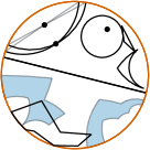
(a)

(b)

(c)

Figure 3: Part (a) shows a visualization of the Poincaré disk including (parallel) lines, a circle with its center, a triangle and generalized polygons. Part (b) shows a visualization of the Beltrami-Klein model including (parallel) lines, a triangle, and a generalized polygon. Part (c) shows a set of sites $S\subseteq\mathbb{H}^{2}$ in the Poincaré disk model, $\mathcal{D}(S)$ (black), and $\mathcal{V}(S)$ (blue); Voronoi vertices are filled squares, ideal Voronoi vertices are empty squares.

We write $\mathbb{H}^{2}$ to refer to the hyperbolic plane and $\mathbb{R}^{2}$ to refer to the Euclidean plane. The Poincaré disk is a model of $\mathbb{H}^{2}$ that maps the whole hyperbolic plane into the interior of a Euclidean unit disk; see 3(a). We refer to the center of the Poincaré disk as origin. Straight lines in $\mathbb{H}^{2}$ are represented as circular arcs perpendicular to the boundary of the Poincaré disk or as chords through the origin. Hyperbolic circles are represented as Euclidean circles. The center of the hyperbolic circle is, however, farther from the origin than the Euclidean center of its representation. The Poincaré disk is conformal, i.e., angle preserving.

Points on the boundary of the Poincaré disk are called ideal points. These are not part of the hyperbolic plane, but form a boundary of infinitely far points. An ideal arc between two ideal points $q_{1}$ and $q_{2}$ is the set of ideal points between $q_{1}$ and $q_{2}$ when moving clockwise on the boundary of the Poincaré disk. A generalized polygon is a cycle together with a planar drawing that maps each vertex to a point in $\mathbb{H}^{2}$ or to an ideal point. Each edge is either a line segments between points, a ray from a point to an ideal point, a line between two ideal points, or an ideal arc between two ideal points. Note that the vertices do not completely determine the generalized polygon, as two ideal points can be connected via a line or an ideal arc. Moreover, a 2-cycle can yield a generalized polygon by mapping both vertices to ideal points and one edge to the line and the other to the ideal arc between the two. Figure 3(a) shows two generalized polygons with their interior shaded in blue.

For a straight line $\ell$ and a point $p\notin\ell$, there are infinitely many parallel lines through $p$, i.e., lines through $p$ that do not intersect $\ell$. Two of these parallel lines are special in the sense that they are the closest to not being parallel. They each share an ideal endpoint with $\ell$ and are called limiting parallels. Let $q\in\ell$ be such that $pq$ is perpendicular to $\ell$. Then the angle between $pq$ and the two limiting parallels is the same on both sides and only depends on the length $x=|pq|$. It is called the angle of parallelism and denoted by $\Pi(x)$. It holds that $\sin(\Pi(x))=1/\cosh(x)$ [20, page 402].

Let $a$ be the sum of interior angles of a hyperbolic triangle. Then $a<\pi$ and the area of the triangle is $\pi-a$. Note that this implies that the area of a triangle is upper bounded by $\pi$. More generally, the area of a $k$-gon is bounded by $(k-2)\pi$. The area of a disk with hyperbolic radius $r$ is $4\pi\sinh^{2}(r/2)$. For $r\to\infty$ this area is in $\Theta(e^{r})$ and for $r\to 0$ it is in $\Theta(r^{2})$.

The Beltrami–Klein model also uses the interior of the Euclidean unit disk as ground space. Hyperbolic straight lines are represented as chords of the unit disk, see Figure 3(b). This model is not conformal, but enables an easy translation of Euclidean line arrangements into the hyperbolic plane.

Delaunay complexes and Voronoi diagrams.

Let $S$ be a set of sites, i.e., a set of designated points in $\mathbb{H}^{2}$. The Voronoi cell of a site $s\in S$ is the set of points that are closer to $s$ than to any other site. When considered in the Poincaré disk, the boundary of each Voronoi cell is a generalized polygon. The non-ideal segments are part of the perpendicular bisector of two sites and are called Voronoi edges; they are illustrated in blue in Figure 3(c). The points in which three or more Voronoi edges meet are called Voronoi vertices. The ideal points in which unbounded Voronoi edges end are called ideal Voronoi vertices. We define the Voronoi diagram $\mathcal{V}(S)$ of $S$ as the following plane graph. Its vertex set is the set of all (ideal) Voronoi vertices. The edge set of $\mathcal{V}(S)$ is comprised of the Voronoi edges and the set of ideal arcs connecting consecutive ideal vertices (red in Figure 3(c)).

The weak dual of the Voronoi diagram is called Delaunay complex and denoted by $\mathcal{D}(S)$; it is illustrated in black in Figure 3(c). The edges of $\mathcal{D}(S)$ are exactly the edges dual to the Voronoi edges, i.e., the edges of $\mathcal{V}(S)$ that are not ideal arcs. Thus, sites $s_{1}\in S$ and $s_{2}\in S$ are connected in the $\mathcal{D}(S)$ if and only if their Voronoi cells share a boundary. In contrast to the Euclidean case, the outer face of $\mathcal{D}(S)$ is not the convex hull of $S$. In fact, its boundary is not necessarily a simple cycle; see Figure 3(c). A site is an outer vertex of $\mathcal{D}(S)$ if and only if the corresponding Voronoi cell is unbounded.

Let $f_{\infty}$ denote the outer face of the Delaunay complex $\mathcal{D}(S)$. For each incidence of an edge $e$ of $\mathcal{D}(S)$ to $f_{\infty}$, the dual edge $e^{\star}$ has one ideal vertex as endpoint. If $e$ is not a bridge, $e^{\star}$ is a ray connecting a Voronoi vertex with an ideal Voronoi vertex. If $e$ is a bridge $e^{\star}$ is a line connecting two ideal Voronoi vertices; one for each incidence of $e$ to $f_{\infty}$.

The Voronoi cells are convex. Thus, drawing each edge $\{u,v\}$ of the Delaunay complex $\mathcal{D}(S)$ by choosing an internal point $p$ on the Voronoi edge dual to $\{u,v\}$ and then connecting $u$ via $p$ to $v$ using the two line segments $up$ and $pv$ yields a planar drawing of $\mathcal{D}(S)$; see Figure 3(c). It has the property that each edge of $\mathcal{D}(S)$ intersects its dual Voronoi edge in exactly one point and it intersects no other Voronoi edges.

3 Balanced separators in HUDGs

Let $G$ be a hyperbolic uniform disk graph with $n$ vertices and radius $r$. We show that $G$ has a balanced separator that can be covered by $\mathcal{O}((1+1/r)\log n)$ cliques; see Theorem 1. The overall argument is as follows. We find a double wedge bounded by two lines $\ell_{1}$ and $\ell_{2}$ that contains no vertex in its interior and separates the other vertices of $G$ in a balanced fashion. In Figure 4(a), the double wedge with apex $p$ is shaded gray and contains no vertices and the regions above and below the wedge each contain a constant fraction of the vertices.

Let $m$ be the angular bisector of the wedge. As separator, we use the set of all vertices that have distance at most $r$ from $m$. The set of points with distance exactly $r$ from $m$ forms two curves that are called hypercycles with axis $m$. Thus, vertices belong to the separator if they lie on or between the two hypercycles. The hypercycles are shown in Figure 4(a) and the region where separator vertices can lie is shaded blue. In the Poincaré disk, hypercycles are arcs of Euclidean circles that meet the boundary of the disk at the same ideal points as their axis but at a non-right angle. Observe that any vertex from above the top hypercycle has distance greater than $2r$ to any vertex below the bottom hypercycle. Thus, the vertices in the blue region indeed form a balanced separator.

It remains to show that the graph induced by vertices in the blue region can be covered with few cliques. For this, we cover the blue region with boxes as shown in Figure 4(b). We show that each of these boxes has diameter at most $2r$, implying that the vertices within one box induce a clique. Moreover, we show that we only need $\mathcal{O}((1+1/r)\log n)$ such boxes. For the latter, we need a lower bound on the opening angle of the empty double wedge. Observe that a larger opening angle $\varphi$ in Figure 4(c) shrinks the blue region, which reduces the number of boxes required to cover it.

In Section 3.1, we give a bound on the number of cliques required to cover the separator, parameterized by the opening angle of the empty double wedge. Afterwards, in Section 3.2 we show that there is a wedge with not too small opening angle that yields a balanced separator. The proof is constructive, i.e., given the graph with vertex positions, we can efficiently find the wedge and thereby a balanced separator.

(a)

(b)

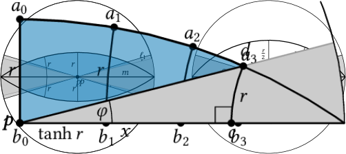
(c)

Figure 4: Illustration of our separator using the Poincaré disk model. (4(a)) The axis $m$ is chosen such that it separates the vertices in a balanced fashion. The double wedge between $\ell_{1}$ and $\ell_{2}$ contains no vertices. The separator consists of the blue set of all vertices of distance at most $r$ to the axis $m$. (4(b)) We cover the separator with boxes that have diameter $2r$ and thus form cliques. (4(c)) If the opening angle $\varphi$ is sufficiently large, then $x$ is sufficiently small and we only need few boxes to cover the whole separator.

3.1 Covering the separator with cliques

We start by defining the boxes between a hypercycle and its axis $m$ as illustrated in Figure 4(b). We place points $b_{0},\dots,b_{k}$ along $m$, such that $b_{0}=p$ and they are evenly spaced at distance $\tanh(r)$. Through each point $b_{i}$ we draw a line perpendicular to $m$ and let $a_{i}$ denote its intersection with the upper hypercycle, see Figure 4(b). We call the region bounded by the line segments $a_{i-1}b_{i-1}$, $b_{i-1}b_{i}$, $b_{i}a_{i}$, and the part of the hypercycle between $a_{i}$ and $a_{i-1}$ a box.

The diameter of each box is at most $2r$.

Proof.

All boxes are congruent as $b_{i-1}a_{i-1}$ and $a_{i}b_{i}$ have length $r$, segment $b_{i-1}b_{i}$ has length $\tanh r$, and there are right angles at $b_{i-1}$ and $b_{i}$. Thus, without loss of generality, we consider only $i=1$.

We first argue that the points realizing the diameter must both be vertices. For this, fix a point $q$ of the box. Let $d$ be the maximum distance of $q$ to a vertex of the box, i.e., the closed disk $D$ of radius $d$ centered at $q$ contains each of the vertices $a_{0},a_{1},b_{0},b_{1}$ (with one of them lying on its boundary). As the sides $a_{0}b_{0}$, $b_{0}b_{1}$, and $b_{1}a_{1}$ are straight line segments and the disk $D$ is convex, these three sides of the box are also contained in $D$ and thus have distance at most $d$ to $q$. The side between $a_{0}$ and $a_{1}$ is not a straight line but a piece of a hypercycle. To see that this side lies also inside $D$, we use that in the Poincaré disk, a hypercycle is a circular arc as shown in Figure 4. Its Euclidean radius in the Poincaré disk is bigger than $1$ (i.e., bigger than that of the Poincaré disk itself). Moreover, the disk $D$ is also a disk in the Poincaré disk, but with smaller radius. Thus, if $a_{0}$ and $a_{1}$ lie in $D$, then the hypercycle segment between $a_{0}$ and $a_{1}$ lies in $D$ and thus has distance at most $d$ form $q$. It follows that the point of the box with maximum distance to $q$ is one of the vertices, which proves the claim that the diameter is realized by two vertices.

It remains to bound the distances between vertices. The length of both sides $a_{0}b_{0}$ and $a_{1}b_{1}$ is $r$ and the length of the side $b_{0}b_{1}$ is $\tanh r<r$. By the triangle inequality, the diagonals have length less than $2r$. It thus remains to bound the length of $a_{0}a_{1}$.

To calculate the distance from $a_{0}$ to $a_{1}$, we can use that the polygon $a_{0},b_{0},b_{1},a_{1}$ is a Saccheri quadrilateral with base $b_{0}b_{1}$ of length $\tanh r$, legs $b_{0}a_{0}$ and $b_{1}a_{1}$ of length $r$, and summit $a_{0}a_{1}$. The length of the summit is given by the following formula [20, Theorem 10.8]:

$$\sinh\frac{|a_{0}a_{1}|}{2} =\cosh r\sinh\frac{\tanh r}{2}$$

$$<\cosh r\sinh\frac{\min\{1,r\}}{2},$$

where we used the simple bound $$\tanh r<\min\{r,1\} r>0 \sinh r\leq 1$$ for and the fact that is strictly increasing. If , then we get

$$\sinh\frac{|a_{0}a_{1}|}{2} <\cosh r\sinh(r/2)$$

$$<2\cosh(r/2)\sinh(r/2)$$

$$=\sinh r,$$

as $$\cosh r<2<2\cosh(r/2) 0<r\leq 1 r>1$$ when . If , then

$$\sinh\frac{|a_{0}a_{1}|}{2} <\cosh r\sinh(1/2)<\sinh r,$$

since $\sinh r/\cosh r=\tanh r>\tanh 1>\sinh(1/2)$ as $\tanh r$ is monotone increasing. Consequently, $|a_{0}a_{1}|<2r$. Thus, all distances between vertices of a box are at most $2r$, which concludes the proof. ∎

From this lemma, it follows that the vertices inside any box induce a clique. Next, we aim to give an upper bound on the number of boxes we need to cover the separator. For this, let $k$ be the smallest number such that $a_{k}$ lies in the wedge formed by $\ell_{1}$ and $\ell_{2}$. In Figure 4(b), $k=3$ as $a_{3}$ lies in the gray wedge. Clearly, we can cover the whole separator (blue in Figure 4), with $\mathcal{O}(k)$ boxes on both sides of the line and thus with $\mathcal{O}(k)$ cliques. The following lemma gives a bound on $k$ depending on the opening angle of the wedge.

Let $k$ be the smallest number such that $a_{k}$ lies inside the wedge with opening angle $2\varphi$. Then the distance between $b_{0}$ and $b_{k}$ is in $\mathcal{O}\big{(}\log\frac{1}{\varphi}\big{)}$.

Proof.

Consider the triangle in Figure 4(c), where $p=b_{0}$ is the apex of the wedge, $d$ is the intersection of the wedge boundary $\ell_{1}$ with the hypercycle, and $c$ is the point on the axis with distance $r$ from $d$. Recall that the distance between $b_{i-1}$ and $b_{i}$ is $\tanh r<1$. Thus, the distance between $b_{0}$ and $b_{k}$ equals the distance $x$ between $p$ and $c$ up to an additive constant. It remains to give an upper bound on $x$.

Using hyperbolic trigonometry of right triangles, we get

$$\tan\varphi=\frac{\tanh r}{\sinh x}\quad\Rightarrow\quad\sinh x=\frac{\tanh r}{\tan\varphi}.$$

Using that $\tanh r<1$ and $\tan\varphi>\varphi$, we obtain $\sinh x<\frac{1}{\varphi}$. This yields the claim. ∎

As the distance between $b_{i-1}$ and $b_{i}$ is $\tanh r$, we can cover the separator with $\mathcal{O}(\log\frac{1}{\varphi}/\tanh r)=\mathcal{O}(\log\frac{1}{\varphi}\cdot(1+1/r))$ many boxes, each of which is covered by one clique. This directly yields the following corollary.

Let $G$ be a hyperbolic uniform disk graph with radius $r$. Let $m$ be a line through a point $p\in\mathbb{H}^{2}$ such that all lines through $p$ and a vertex of $G$ have an angle of at least $\varphi$ with $m$. Then the subgraph of $G$ induced by vertices of distance at most $r$ from $m$ can be covered with $\mathcal{O}\big{(}\log\frac{1}{\varphi}\cdot(1+\frac{1}{r})\big{)}$ cliques.

3.2 Balanced separators

Corollary 3.1 already yields a separator that can be covered with few cliques, if the angle $\varphi$ is not too small. It remains to provide the point $p$ together with the line $m$ through $p$ such that the separator is balanced and $\varphi$ is not too small. For this, let $V$ be a set of $n$ points (the vertices of $G$). We call a point $p\in\mathbb{H}^{2}$ a centerpoint of $V$ if every line through $p$ divides $V$ into two subsets that both have size at least $\frac{n}{3}$. The following lemma provides such a centerpoint (which follows directly from the existence of a Euclidean centerpoint [26]). It was also observed in [27], but we provide a proof for completeness.

[See also [27, proof of Lemma 4]] A centerpoint of a set of $n$ points in the hyperbolic plane exists and can be found in $\mathcal{O}(n)$ time.

Proof.

We do this by first converting the points to the Beltrami-Klein model of the hyperbolic plane. Here, any hyperbolic line is also a Euclidean line, which means a Euclidean centerpoint is also a hyperbolic centerpoint. Thus, we can simply find the Euclidean centerpoint (which takes $\mathcal{O}(n)$ time [26]) and then convert it back to our original model of the hyperbolic plane. ∎

Now, consider the lines $\ell_{1},\dots,\ell_{n}$, where $\ell_{i}$ goes through $p$ and the vertex $v_{i}\in V$. Let without loss of generality $\ell_{1}$ and $\ell_{2}$ be the two consecutive lines with maximum angle between them. As there are $2n$ angles between consecutive lines covering the full $2\pi$ angle, the angle between $\ell_{1}$ and $\ell_{2}$ is at least $\pi/n$. Set $m$ to be the angular bisector of $\ell_{1}$ and $\ell_{2}$. It follows that $\frac{1}{\varphi}\in\mathcal{O}(n)$ and thus Corollary 3.1 yields a separator that can be covered by $\mathcal{O}(\log n\cdot(1+\frac{1}{r}))$ cliques. Moreover, as $m$ goes through the centerpoint $p$, this separator is balanced. Clearly, the line $m$ and thus the separator can be computed in $\mathcal{O}(n\log n)$ time. This concludes the proof of Theorem 1.

See 1

4 Outerplanarity of hyperbolic Delaunay complexes

Let $S$ be a set of $n$ sites in $\mathbb{H}^{2}$ with pairwise distance at least $2r$. Note that $S$ interpreted as hyperbolic uniform disk graph with radius $r$ forms an independent set. Here we prove Theorem 2, giving an upper bound on the outerplanarity of the Delaunay complex $\mathcal{D}(S)$. We use two different types of arguments. The first argument is, roughly speaking, based on the observation that any inner vertex of $\mathcal{D}(S)$ requires many other sites around it to shield it from being an outer vertex. This is similar to the observation in the introduction (recall Figure 1) that for high radius $r$, large stars can be realized. Consequentially, this first type of argument only works in case $r$ is a sufficiently large constant. The second type of argument considers layers of bounded Voronoi cells (which correspond to inner vertices of $\mathcal{D}(S)$) around one fixed center cell. As the union of these layers is bounded by a polygon with a linear number of vertices, its area is linear. In contrast to that, we will see that the area of the layers grows exponentially with the layer (with the base depending on $r$), showing that there cannot be too many layers.

Before we start with the proof, we make one more observation. If the sites $S$ are in general position, i.e., no four sites lie on the same circle, then the Voronoi diagram is a $3$-regular graph and the Delaunay complex is internally triangulated, i.e., each inner face is a triangle. Otherwise, the sites $S$ can be slightly perturbed to give a set $S^{\prime}$, such that $\mathcal{D}(S^{\prime})$ is obtained from $\mathcal{D}(S)$ by triangulating each inner face. Moreover $\mathcal{V}(S^{\prime})$ is obtained from $\mathcal{V}(S)$ by splitting each vertex of degree more than $3$ into a binary tree. Triangulating $\mathcal{D}(S)$ only adds edges to it and thereby only increases its outerplanarity. Thus, any upper bound on the outerplanarity of $\mathcal{D}(S^{\prime})$ also holds for $\mathcal{D}(S)$. For this section, we assume without loss of generality that $S$ is in general position, i.e., $\mathcal{D}(S)$ is internally triangulated.

4.1 Large-radius case

We start with the argument for the case where the radius is sufficiently large. The core observation that any inner vertex of $\mathcal{D}(S)$ requires many other sites around it is summarized in the following lemma.

Let $S$ be a set of sites in $\mathbb{H}^{2}$ with pairwise distance at least $2r$. Any inner vertex of the Delaunay complex $\mathcal{D}(S)$ has degree at least $e^{r}$.

Proof.

Let $s\in S$ be a site that is an inner vertex of $\mathcal{D}(S)$, i.e., its Voronoi region is bounded. We show that the angle between consecutive neighbors of $s$ must not to be too large as the Voronoi region of $s$ would be unbounded otherwise. Consider two consecutive neighbors $a,b\in S$ of $s$ as shown in Figure 5. Let $p_{a}$ and $p_{b}$ be the perpendicular bisectors of $sa$ and $sb$, respectively, and let $\ell$ be the angular bisector of $sa$ and $sb$. Since $s$ is an inner vertex, $p_{a}$ and $p_{b}$ have to intersect and thus $p_{a}$ or $p_{b}$ has to intersect $\ell$.

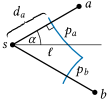
Figure 5: Illustration of Lemma 4.1. An inner vertex of the Delaunay complex $s$ with two consecutive neighbors $a$ and $b$. From the fact that the Voronoi cell of $s$ is bounded, we can derive an upper bound for the angle $2\alpha$ between $sa$ and $sb$.

Without loss of generality assume that $p_{a}$ intersects $\ell$, as in Figure 5. Because all sites in $S$ have pairwise distance at least $2r$, the distance $d_{a}$ between $s$ and the intersection of $sa$ with its perpendicular bisector $p_{a}$ is at least $r$. The angle $\alpha$ between $sa$ and $\ell$ has to be smaller than the angle of parallelism $\Pi(d_{a})$, as $\ell$ and $p_{a}$ intersect. Thus, we get

$$\alpha<\Pi(d_{a})\leq\frac{\pi}{2}\sin\Pi(d_{a})=\frac{\pi}{2}\frac{1}{\cosh d_{a}}\leq\pi e^{-d_{a}}\leq\pi e^{-r}.$$

Therefore, the angle between $sa$ and $sb$ is at most $2\alpha\leq 2\pi e^{-r}$. It follows that $s$ has at least $\frac{2\pi}{2\pi e^{-r}}=e^{r}$ neighbors. ∎

Observe that if $r>\log 6$, then every inner vertex of $\mathcal{D}(S)$ has degree more than $6$. As the average degree in planar graphs is at most $6$, a constant fraction of vertices have to be outer vertices to make up for the above-average degree of inner vertices. This observation yields the following lemma.

Let $G$ be a plane graph in which every inner vertex has degree at least $d>6$. Then $G$ is $k$-outerplanar for $k<1+\log_{d/6}n$.

Proof.

In a planar graph with $n$ vertices, Euler’s formula implies that the number of edges is less than $3n$. Thus the sum of all vertex degrees is less than $6n$. Let $n_{\text{inner}}$ be the number of inner vertices. As the sum of inner degrees, which is at least $d\cdot n_{\text{inner}}$, is at most the sum of all degrees, we get $d\cdot n_{\text{inner}}\leq 6n$. Consequently, $n_{\text{inner}}<n\cdot 6/d$.

It follows that removing all outer vertices yields a plane graph with less than $n\cdot 6/d$ vertices in which every inner vertex again has degree at least $d$. Thus, repeatedly removing all outer vertices $k$ times yields a graph with less than $n\cdot(6/d)^{k}$ vertices. Hence $G$ is reduced to at most one vertex in less than $\log_{d/6}n$ rounds, which concludes the proof. ∎

For $r\geq 1.8>\log 6$, these two lemmas already yield the claim of Theorem 2; also see the formal proof in Section 4.3, where we combine the large- and small-radius case.

4.2 Small-radius case

As mentioned above, we use an argument based on area for the case that the radius is a small constant or even decreasing with $n$. Before we start, we give a simple area-based argument for why $r\geq\log n$ implies that the Delaunay complex has no inner vertices. Although our argument for small radii is more involved, this gives a good intuition how the area behaves in the hyperbolic plane and how this can help us in proving outerplanarity. Let $s\in S$ be a site. If $s$ is an inner vertex of $\mathcal{D}(S)$, then its Voronoi cell is bounded and its boundary is a polygon of at most $n-1$ vertices. Thus, the area of this Voronoi cell is less than $(n-3)\pi$. Simultaneously, the disk of radius $r$ around $s$ is included in the Voronoi cell of $s$ as all sites have pairwise distance at least $2r$. The area of this disk is $4\pi\sinh^{2}(\frac{r}{2})$ which is larger than $e^{r}$ for sufficiently large $r$. From this it follows that bounded cells can only exist when $r<\log n$.

To make an argument that works for smaller $r$, let $s\in S$ be an arbitrary but fixed vertex of the Delaunay complex $\mathcal{D}(S)$. We partition the vertices of $\mathcal{D}(S)$ into layers by hop distance from $s$ in $\mathcal{D}(S)$, i.e., $V_{\ell}$ is the set of vertices with distance $\ell$ from $s$. Let $L$ be the largest integer such that for all $\ell\leq L$ the layer $V_{\ell}$ contains only inner vertices. Note that our goal is to prove an upper bound on $L$ as this bounds the distance of $s$ to the outer face.

As the Delaunay complex is an internally triangulated plane graph, each layer $V_{\ell}$ induces a cycle. We denote the vertices in $V_{\ell}$ with $v_{\ell}^{i}$ and number the vertices modulo $|V_{\ell}|$, such that vertex $v_{\ell}^{i}$ is adjacent to vertices $v_{\ell}^{i-1}$ and $v_{\ell}^{i+1}$; see Figure 6(a). Moreover, we assume the Delaunay graph to be drawn as follows. For every edge $\{v_{\ell}^{i},v_{\ell}^{i+1}\}$ we choose a point on its dual edge, i.e., the boundary between the two corresponding Voronoi cells, denote it with $v_{\ell}^{i+0.5}$, and connect $v_{\ell}^{i}$ and $v_{\ell}^{i+1}$ with two line segments via $v_{\ell}^{i+0.5}$. We denote the resulting polygon with $P_{\ell}$ and call it a layer polygon of $s$. Note that this yields a sequence of nested polygons where $P_{\ell-1}$ lies in the interior of $P_{\ell}$.

(a)

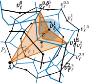
(b)

(c)

Figure 6: Illustration of the small-radius case. (a) shows two consecutive layer polygons $P_{\ell-1}$ and $P_{\ell}$ in the Delaunay complex around $s$. The Voronoi diagram is shown in blue. We show an upper bound of the area inside $P_{\ell}$ by covering it with the red triangles (b). We show a lower bound for the area between $P_{\ell-1}$ to $P_{\ell}$ via the red triangles in (c). Relating these two bounds yields an exponential area growth with a basis depending on $r$.

Our goal then is to show that the area inside $P_{\ell}$, denoted by $\operatorname{\mathrm{Area}}(P_{\ell})$, grows exponentially in $\ell$ with a basis $b(r)$ depending on $r$. As $\operatorname{\mathrm{Area}}(P_{L})$ for the outermost layer $L$ is upper bounded by something linear in $n$, there cannot be too many layers. The interesting part is proving the exponential growth. For this, we show that the area gain $\operatorname{\mathrm{Area}}(P_{\ell})-\operatorname{\mathrm{Area}}(P_{\ell-1})$ in layer $\ell$ makes up at least some sufficiently large fraction of the area $\operatorname{\mathrm{Area}}(P_{\ell})$. For this, we give an upper bound for $\operatorname{\mathrm{Area}}(P_{\ell})$ and relate it to a lower bound for $\operatorname{\mathrm{Area}}(P_{\ell})-\operatorname{\mathrm{Area}}(P_{\ell-1})$.

How we derive these bounds is illustrated in Figure 6(b) and Figure 6(c), respectively. For the upper bound on $\operatorname{\mathrm{Area}}(P_{\ell})$, we cover $P_{\ell}$ with triangles connecting every edge of $P_{\ell}$ with the vertex $s$; see the two red triangles in Figure 6(b) for the two edges $\{v_{\ell}^{0.5},v_{\ell}^{1}\}$ and $\{v_{\ell}^{1},v_{\ell}^{1.5}\}$ of $P_{\ell}$. For the lower bound, we find a set of disjoint triangles that lie between $P_{\ell}$ and $P_{\ell-1}$. For this, observe that for every vertex $v_{\ell}^{i}\in V_{\ell}$ in layer $\ell$, the Voronoi cell of $v_{\ell}^{i}$ completely contains the disk of radius $r$ around $v_{\ell}$ as the sites have pairwise distance at least $2r$. Thus, the two triangles illustrated in red for $v_{\ell}^{1}$ in Figure 6(c) satisfy the property of lying between $P_{\ell}$ and $P_{\ell-1}$. As the two triangles can in principle intersect, we choose for each vertex in layer $\ell$ the larger of the two triangles. Note that this gives a collection of $|V_{\ell}|$ disjoint triangles, as each chosen triangle lies in a different Voronoi cell. Thus, the total area of these triangles gives a lower bound for $\operatorname{\mathrm{Area}}(P_{\ell})-\operatorname{\mathrm{Area}}(P_{\ell-1})$.

It then remains to relate the upper bound for $\operatorname{\mathrm{Area}}(P_{\ell})$, i.e., the area of the red triangles in Figure 6(b), with the lower bound for $\operatorname{\mathrm{Area}}(P_{\ell})-\operatorname{\mathrm{Area}}(P_{\ell-1})$, i.e., the area of larger red triangle in Figure 6(c). Intuitively, this does not seem too far fetched for the following reasons. First, the triangles in Figure 6(b) share a side with the triangles in Figure 6(c). Secondly, the other sides of the triangles in Figure 6(c) have length at least $r$. Thus, the triangles in Figure 6(c) cannot be too much smaller than those in Figure 6(b).

Before formalizing the above proof idea, we show two simple results about hyperbolic triangle areas, both based on the fact that a right-angled triangle with short sides of length $a$ and $b$ has area $2\arctan\left(\tanh\frac{a}{2}\cdot\tanh\frac{b}{2}\right)$. We start with an upper bound on the area of a triangle where one side has a specific length. This will serve as an upper bound for the triangles in Figure 6(b).

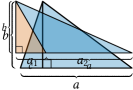
(a)

(b)

Figure 7: Illustration of Lemma 4.2 giving an upper bound on the area of a triangle (blue) with side length $a$.

Any triangle with one side of length $a$ has area at most $\min\{a,\pi\}$.

Proof.

We first need that $\arctan(\tanh x)\leq\min\{x,\pi/4\}$ for $x\geq 0$. Here, $\tanh x<1$ implies $\arctan(\tanh x)<\arctan 1=\pi/4$ as $\arctan$ is strictly increasing. For the other part, using that $\tanh(x)\leq x$ and $\arctan(x)\leq x$ for $x\geq 0$ yields $\arctan(\tanh x)\leq\tanh x\leq x$.

Consider the line perpendicular to the side of length $a$ through its opposite vertex. It either splits the triangle in two right triangles as shown in Figure 7(a) or it extends the triangle into a larger one as shown in Figure 7(b). In both cases, let $b$ be the length of the new perpendicular line. Moreover, in the first case, the side of length $a$ is split into two sides of length $a_{1}$ and $a_{2}$. In the second case, the side of length $a$ is extended by $c$ yielding a right triangle with side length $c+a$.

For the first case, the area of the triangle (blue in Figure 7(a)) is the sum of the two triangles, i.e.,

$$2\arctan\left(\tanh\frac{a_{1}}{2}\tanh\frac{b}{2}\right)+2\arctan\left(\tanh\frac{a_{2}}{2}\tanh\frac{b}{2}\right) \leq 2\arctan\left(\tanh\frac{a_{1}}{2}\right)+2\arctan\left(\tanh\frac{a_{2}}{2}\right)$$

$$\leq\min\{a_{1},\pi/2\}+\min\{a_{2},\pi/2\}$$

$$\leq\min\{a,\pi\}.$$

For the second case, we are interested in the area of the blue triangle in Figure 7(b). Using that $\arctan(x)$ and $\tanh(x)$ are both subadditive for $x\geq 0$ and $\arctan$ is increasing, we can estimate the area of the right triangle with side lengths $b$ and $c+a$ ($\text{red}+\text{blue}$ in Figure 7(b)) as

$$2\arctan\left(\tanh\frac{a+c}{2}\tanh\frac{b}{2}\right) \leq 2\arctan\left(\left(\tanh\frac{a}{2}+\tanh\frac{c}{2}\right)\tanh\frac{b}{2}\right)$$

$$\leq 2\arctan\left(\tanh\frac{a}{2}\tanh\frac{b}{2}\right)+2\arctan\left(\tanh\frac{c}{2}\tanh\frac{b}{2}\right).$$

Now we get the area of the triangle with side length $a$ (blue), as the difference between two right triangles ($\text{red}+\text{blue}-\text{red}$), which yields

$$2\arctan\left(\tanh\frac{a+c}{2}\tanh\frac{b}{2}\right)-2\arctan\left(\tanh\frac{c}{2}\tanh\frac{b}{2}\right) \leq 2\arctan\left(\tanh\frac{a}{2}\tanh\frac{b}{2}\right)$$

$$\leq 2\arctan\left(\tanh\frac{a}{2}\right)$$

$$\leq\min\{a,\pi\}.\qed$$

To lower bound the area of the triangles in Figure 6(c), we use the following lemma. We note that the requirement $a\leq 1.8$ in this lemma is the reason why this section only deals with the case $r\leq 1.8$.

A right-angled triangle with short sides of length $a\leq 1.8$ and $b$ has area at least $a/5\cdot\min\{b,\pi\}$.

Proof.

The area is given by the function $f_{b}(a):=2\arctan\left(\tanh\frac{a}{2}\cdot\tanh\frac{b}{2}\right)$, which is concave, as $f_{b}^{\prime\prime}(a)=-\frac{2\sinh a\sinh(2b)}{(2+2\cosh a\cosh b)^{2}}\leq 0$ for any $a,b\in\mathbb{R}$. Because additionally $f_{b}(0)=0$, we can say that $f_{b}(a)\geq a\cdot f_{b}(1.8)/1.8$ for $a\in[0,1.8]$. What remains is to bound $g(b):=f_{b}(1.8)$. This function $g(b)$ is concave for analogous reasons as before, and again $g(0)=0$, so we can say that $g(b)\geq b\cdot g(\pi)/\pi\geq 0.37b$ for $b\in[0,\pi]$. Additionally, $g(b)\geq 0.37\pi$ for $b\geq\pi$. Thus, $f_{b}(a)\geq a/5\cdot\min\{b,\pi\}$ for $a\in[0,1.8]$. ∎

With this, we are ready to show that the area of the layer polygons grows exponentially.

Let $r\leq 1.8$ and let $S$ be a set of sites in $\mathbb{H}^{2}$ with pairwise distance at least $2r$. Let $s\in S$ be any site and let $P_{\ell}$ be the $\ell$-th layer polygon of $s$ in the Delaunay complex $\mathcal{D}(S)$. Then $\operatorname{\mathrm{Area}}(P_{\ell})\geq\frac{10}{10-r}\cdot\operatorname{\mathrm{Area}}(P_{\ell-1})$.

Proof.

We give an upper bound on $\operatorname{\mathrm{Area}}(P_{\ell})$ as well as a lower bound on $\operatorname{\mathrm{Area}}(P_{\ell})-\operatorname{\mathrm{Area}}(P_{\ell-1})$ and then relate these two. For the upper bound on $\operatorname{\mathrm{Area}}(P_{\ell})$, we cover $P_{\ell}$ with triangles as shown in Figure 6(b) and sum the area of these triangles. For each $v_{i}\in V_{\ell}$, we get two triangles with sides $v_{\ell}^{i-0.5}v_{\ell}^{i}$ and $v_{\ell}^{i}v_{\ell}^{i+0.5}$, respectively. Using Lemma 4.2 to bound their area, we obtain

$$\operatorname{\mathrm{Area}}(P_{\ell})\leq\sum_{i=1}^{|V_{\ell}|}\min\{|v_{\ell}^{i-0.5}v_{\ell}^{i}|,\pi\}+\min\{|v_{\ell}^{i}v_{\ell}^{i+0.5}|,\pi\}.$$

For the lower bound, let $v_{i}\in V_{\ell}$ and consider the triangle with a right angle at $v_{\ell}^{i}$ where the two sides forming that right angle are $v_{\ell}^{i}v_{\ell}^{i+0.5}$ and the perpendicular line segment of length $r$ that lies in the interior of $P_{\ell}$; see Figure 6(c). Analogously, we define a triangle with side $v_{\ell}^{i+0.5}v_{\ell}^{i}$. Using Lemma 4.2 the larger of the two triangles has area at least $r/5\cdot\min\big{\{}\max\{|v_{\ell}^{i-0.5}v_{\ell}^{i}|,|v_{\ell}^{i}v_{\ell}^{i+0.5}|\},\ \pi\big{\}}$, which is at least $r/10\cdot\big{(}\min\{|v_{\ell}^{i-0.5}v_{\ell}^{i}|,\pi\}+\min\{|v_{\ell}^{i}v_{\ell}^{i+0.5}|,\pi\}\big{)}$. Note that these two triangles lie inside $P_{\ell}$ but outside $P_{\ell-1}$ and they do not intersect other triangles that are obtained in the same way for other vertices in $V_{\ell}$. Thus, we obtain

$$\operatorname{\mathrm{Area}}(P_{\ell})-\operatorname{\mathrm{Area}}(P_{\ell-1})\geq\frac{r}{10}\sum_{i=1}^{|V_{\ell}|}\min\{|v_{\ell}^{i-0.5}v_{\ell}^{i}|,\pi\}+\min\{|v_{\ell}^{i}v_{\ell}^{i+0.5}|,\pi\}.$$

Observe that this lower bound is the same as the upper bound except for the factor of $r/10$. Thus, we obtain $\operatorname{\mathrm{Area}}(P_{\ell})-\operatorname{\mathrm{Area}}(P_{\ell-1})\geq\frac{r}{10}\operatorname{\mathrm{Area}}(P_{\ell})$. Rearranging yields the claimed bound. ∎

4.3 Combining the two

Combining the results for small and large radius, we obtain the desired theorem.

See 2

Proof.

First, assume $r\geq 1.8$. As $1.8>\log 6$, it follows from Lemma 4.1 that any inner vertex of $\mathcal{D}(S)$ has degree at least $e^{r}>6$. We can thus apply Lemma 4.1 to obtain that $\mathcal{D}(S)$ is $k$-outerplanar for $k<1+\log_{e^{r}/6}n$, which matches the claimed bound.

For the case where $r\leq 1.8$, first note that the claimed bound trivially holds for $r\leq 1/n$ as any planar graph is clearly $\mathcal{O}(n\log n)$-outerplanar. For $1/n<r\leq 1.8$, let $s\in S$ be any site and consider the layer polygons $P_{1},\dots,P_{L}$ where $L+1$ is the distance of $s$ in $\mathcal{D}(S)$ to the closest outer vertex. Then by Lemma 4.2 the area of the polygons grows by a factor of at least $\frac{10}{10-r}$ in every step and thus we get

$$\left(\frac{10}{10-r}\right)^{L}\cdot\operatorname{\mathrm{Area}}(P_{1})\leq\operatorname{\mathrm{Area}}(P_{L})\quad\Rightarrow\quad L\leq\frac{\log\frac{\operatorname{\mathrm{Area}}(P_{L})}{\operatorname{\mathrm{Area}}(P_{1})}}{\log\frac{10}{10-r}}.$$

First note that $\log\frac{10}{10-r}\geq\frac{r}{10}$ for $r<10$ and thus it remains to show that $\frac{\operatorname{\mathrm{Area}}(P_{L})}{\operatorname{\mathrm{Area}}(P_{1})}$ is polynomial in $n$. For this observe that $\operatorname{\mathrm{Area}}(P_{L})\leq 2\pi n$ as it is a polygon with less than $2n$ vertices. Moreover, $P_{1}$ at least includes the Voronoi cell of $s$, which includes a disk of radius $r$ as sites have pairwise distance at least $2r$. Thus, $\operatorname{\mathrm{Area}}(P_{1})\geq 4\pi\sinh^{2}(r/2)\in\Omega(1/n^{2})$ as $r\geq 1/n$ and $\sinh x$ behaves like $x$ for $x$ close to $0$. It follows that $L\in\mathcal{O}\big{(}\frac{\log n}{r}\big{)}$, which concludes the proof. ∎

5 Exact algorithm for Independent Set

In the following, we give an exact algorithm for computing an independent set of a given size in a hyperbolic uniform disk graph $G$ of radius $r$ that is given via its geometric realization. Let $S$ be an independent set of $G$. As there are no edges between vertices in $S$, they have pairwise distance at least $2r$. Thus, Theorem 2 gives us an upper bound on the outerplanarity of the Delaunay complex $\mathcal{D}(S)$, which implies that $\mathcal{D}(S)$ has small treewidth and thereby small balanced separators. In a nutshell, our algorithm first lists all relevant separators of the Delaunay complexes of all possible independent sets. We then use a dynamic program to combine these candidate separators into a hierarchy of separators, maximizing the number of vertices of the corresponding Delaunay complex and thereby the size of the independent set $S$.

A crucial tool for dealing with these separators are sphere cut decompositions. They are closely related to tree decompositions but represent the separators as closed curves called nooses. We introduce sphere cut decompositions in Section 5.1. Afterwards, in Section 5.2 we define normalized geometric realizations of nooses for sphere cut decompositions of Delaunay complexes. In Section 5.3, we prove that there are not too many candidate nooses and that selecting a subset of candidate nooses that can be combined into a hierarchy of separators actually yields an independent set. Finally, in Section 5.4, we describe the dynamic program for computing the independent set, which follows almost immediately from the previous sections.

5.1 Sphere cut decompositions

A branch decomposition [42] of a graph $G$ is an unrooted binary tree $T$, i.e., each non-leaf node has degree exactly 3, and there is a bijection between the leaves of $T$ and the edges of $G$. Observe that removing an edge $e_{T}\in E(T)$ separates $T$ into two subtrees and thereby separates its leaves and thus the edges of $G$ in two subsets. Let $E_{1}\subset E(G)$ and $E_{2}\subset E(G)$ be these two edge sets and let $G[E_{1}]$ and $G[E_{2}]$ be their induced subgraphs. The vertices shared by $G[E_{1}]$ and $G[E_{2}]$, i.e., vertices that appear in edges of $E_{1}$ and of $E_{2}$, are called the middle set of $e_{T}$. The width of the branch decomposition $T$ is the size of the largest middle set over all edges of $T$. The branch-width of $G$ is the minimum width of all branch decompositions of $G$. Robertson and Seymour [42] showed that the branch-width of a graph is within a constant factor of its treewidth.

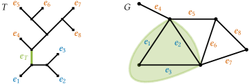
Figure 8: A branch decomposition $T$ of a graph $G$ with a highlighted edge $e_{T}$ of $T$ and the corresponding noose in $G$, that separates the two parts of $E(G)$.

If $G$ is a plane graph, results by Seymour and Thomas [43] imply that we can wish for some additional structure without increasing the width of the branch decomposition [16, 37]. Specifically, a sphere cut decomposition of a plane graph $G$ is a branch decomposition $T$ such that every tree edge $e_{T}\in E(T)$ is associated with a so-called noose. The noose $O$ of $e_{T}$ is a simple closed curve that intersects the vertices of $G$ exactly in the middle set of $e_{T}$ and separates $G[E_{1}]$ from $G[E_{2}]$; see also Figure 8. Moreover, removing the vertices of the middle set from $O$ separates $O$ into noose segments such that each segment lies entirely in the interior of a face of $G$ and every face contains at most one noose segment, except if $E_{1}$ or $E_{2}$ contains just a bridge of $G$. In the latter case, the noose consists of two noose segments through the face incident to the bridge. It should be mentioned that this differs from the original definition by Dorn, Penninkx, Bodlaender and Fomin [16]. Here, a noose may intersect any face at most once and thus the graph cannot have bridges, as discussed by Marx and Pilipczuk [37]. With our relaxed definition of nooses however, we get the following theorem.

Theorem 5 ([16, 37]).

Let $G$ be a plane graph with branch-width $b$. Then $G$ has a sphere cut decomposition, where every noose intersects at most $b$ vertices of $G$.

In the following, we assume sphere cut decompositions to be rooted at a leaf node. Let $e_{T}\in E(T)$ be a tree edge between $u_{T}\in V(T)$ and $v_{T}\in V(T)$ such that $u_{T}$ is the parent of $v_{T}$. Moreover, let $G[E_{1}]$ and $G[E_{2}]$ be the two subgraphs defined by $e_{T}$ and assume that $E_{1}$ corresponds to the leaves that are descendants of the child $v_{T}$ in $T$. Then, we call the side of the noose $O$ of $e_{T}$ that contains $G[E_{1}]$ its interior and the side containing $G[E_{2}]$ its exterior. We note that, if the root of $T$ is appropriately chosen, this corresponds to the typical definition of interior and exterior of closed curves in the plane. In the following, when specifying a noose (or a closed curve that could be a noose), its interior and exterior is implicitly given by assuming a clockwise orientation, i.e., we assume that the interior of a noose lies to its right when traversing it in the given orientation.

We note that rooting the sphere cut decomposition also defines a child–parent relation on the nooses. Consider a non-leaf node $v_{T}\in V(T)$. It has an edge $e_{P}$ to the parent, and two edges $e_{L}$ and $e_{R}$ to the left and right child corresponding to the nooses $O_{P}$, $O_{L}$, and $O_{R}$, respectively. We say that $O_{P}$ is the parent noose of the child nooses $O_{L}$ and $O_{R}$. Note that the subgraph in the interior of $O_{P}$ is the union of the subgraphs in the interior of $O_{L}$ and $O_{R}$.

5.2 Geometric nooses of Delaunay complexes

In this section, we are interested in the sphere cut decomposition of the Delaunay complex $\mathcal{D}(S)$ of a set of sites $S$. When working with a sphere cut decomposition, the exact geometry of the nooses is often not relevant, i.e., it is sufficient to know that there exists a closed curve with the desired topological properties. In our case, however, the geometry is actually important. Our goal here is the following. Given a noose $O$ of a sphere cut decomposition of $\mathcal{D}(S)$, we define a normalized geometric realization of $O$, i.e., a fixed closed curve satisfying the noose requirements. Afterwards, we will observe that this normalized realization has some nice properties.

Our normalized nooses will be generalized polygons (recall the definition in Section 2). We note that generalized polygons are technically not closed curves in the hyperbolic plane. However, they are closed curves in the Poincaré disk when perceived as a disk of the Euclidean plane. Thus, generalized polygons are suited to represent nooses.

(a)

(b)

(c)

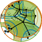
(d)

Figure 9: Part (a): Delaunay complex $\mathcal{D}(S)$ (black) together with the corresponding Voronoi diagram (blue). Part (b) visualizes the choice of the ideal point $p_{u}$ for a Voronoi ray, as needed for the normalization of the green noose. Part (c) shows the normalized version of the noose from part (b) alongside two other normalized nooses, each separating a single edge of $\mathcal{D}(S)$. Observe that the depicted normalized nooses include zero, one, or two ideal arcs, respectively. Part (d) shows a parent noose (green) and its child nooses, with interiors colored orange and blue.

To define the normalized nooses, let $O$ be a noose and consider an individual noose segment of $O$ that goes from $u$ to $v$ (which are vertices of $\mathcal{D}(S)$) through the face $f$ of $\mathcal{D}(S)$. If $f$ is an inner face, then $f$ corresponds to a vertex of the Voronoi diagram $\mathcal{V}(S)$. Let $p_{f}$ be the position of this vertex. Then, the normalized noose segment from $u$ to $v$ through $f$, consists of the two straight line segments from $u$ to $p_{f}$ and from $p_{f}$ to $v$.

If $f=f_{\infty}$ is the outer face, $u$ and $v$ can have multiple incidences to $f_{\infty}$ (in fact $u$ and $v$ could be the same vertex). To make the situation more precise, assume that we traverse the boundary of $f_{\infty}$ such that $f_{\infty}$ lies to the left and let $e_{u}$ be the edge incident to $f_{\infty}$ that precedes the incidence of $u$ where the noose enters $f_{\infty}$; see Figure 9(b). Recall that the dual Voronoi edge $e_{u}^{\star}$ is unbounded and ends in some ideal point $p_{u}$. Let $e_{v}$ and $p_{v}$ be defined analogously for $v$. Then, for the normalized noose segment from $u$ to $v$ in $f_{\infty}$, we use the ray between $u$ and $p_{u}$, the ideal arc from $p_{u}$ to $p_{v}$, and the ray between $p_{v}$ and $v$.

Observe that combining the geometric noose segments as defined above yields a generalized polygon for each noose; see Figure 9(c). Also, note that this definition also works in the special case where the noose goes only through one vertex with two incidences to the outer face, in which case the noose consists of just two rays and an ideal arc.

It is easy to observe that the above construction in fact yields geometric realizations of the nooses, i.e., the resulting curves have the desired combinatorial properties in regards to which elements of $\mathcal{D}(S)$ lie inside, outside, or on a noose. We call a sphere cut decomposition of $\mathcal{D}(S)$, with such normalized nooses a normalized sphere cut decomposition. In the following, we summarize properties of these nooses that we need in later arguments. The first lemma follows immediately from the construction above.

Let $S$ be a set of sites with Delaunay complex $\mathcal{D}(S)$ and Voronoi diagram $\mathcal{V}(S)$. Let $O$ be a noose of a normalized sphere cut decomposition of $\mathcal{D}(S)$. Then $O$ is a generalized polygon and each vertex of $O$ is either a site, a vertex of $\mathcal{V}(S)$, or an ideal vertex of $\mathcal{V}(S)$. Between any two subsequent sites visited by $O$, there is either exactly one vertex of $\mathcal{V}(S)$ or two ideal vertices of $\mathcal{V}(S)$ in $V(O)$. In the latter case, the ideal vertices are connected via an ideal arc.

The previous lemma summarizes the core properties of individual nooses. Next, we describe additional properties of how nooses interact in their parent-child relationships. See also Figure 9(d).

Let $S$ be a set of sites with Delaunay complex $\mathcal{D}(S)$. Let $O_{P}$, $O_{L}$, and $O_{R}$ be three nooses of a normalized sphere cut decomposition of $\mathcal{D}$ such that $O_{P}$ is the parent noose of $O_{L}$ and $O_{R}$. Then $O_{L}$, $O_{R}$ and $O_{P}$ intersect in exactly two points $p_{1}$, $p_{2}$ and $O_{P}\setminus\{p_{1},p_{2}\}$ is the symmetric difference of $O_{L}$ and $O_{R}$. Further, the interiors of $O_{L}$ and $O_{R}$ are subsets of the interior of $O_{P}$.

Proof.

To prove this, we consider how the nooses separate the graph. There is an internal node of the sphere cut decomposition that is incident to the three edges associated with $O_{P}$, $O_{L}$, and $O_{R}$ and this internal node separates the edges of $\mathcal{D}(S)$ into three parts $E_{P}$, $E_{L}$, and $E_{R}$ such that in $\mathcal{D}(S)$ the noose $O_{P}$ separates $E_{L}\cup E_{R}$ from $E_{P}$, $O_{L}$ separates $E_{L}$ from $E_{R}\cup E_{P}$, and $O_{R}$ separates $E_{R}$ from $E_{P}\cup E_{L}$.

The faces visited by $O_{L}$ are exactly those faces of $\mathcal{D}(S)$ whose boundary contains edges both from $E_{L}$ and from $E_{R}\cup E_{P}$, and analogous statements hold for $O_{R}$ and $O_{P}$. This means that any noose that separates, e.g., $E_{L}$ from the rest of the graph has to pass through a uniquely determined set of vertices and faces in a uniquely determined cyclic order. For two nooses that visit a shared set of faces, the cyclic order in which these faces and the incident vertices are visited thus has to coincide. We can thus consider a combinatorial representation $O^{\star}_{L}$, $O^{\star}_{R},$ and $O^{\star}_{P}$ of the three nooses as a cyclic order of vertex-face-incidences and it follows that $O^{\star}_{P}$ is the symmetric difference of $O^{\star}_{L}$ and $O^{\star}_{R}$. For a vertex-face-incidence of a combinatorial noose, its normalized geometric realization contains a line segment or ray that is uniquely determined by the vertex and face according to the construction of normalized nooses. This implies that $O_{P}$ is the symmetric difference of $O_{L}$ and $O_{R}$, except for exactly two points that are visited by all three normalized nooses. These correspond either to a vertex of $\mathcal{D}(S)$ at which all three nooses meet or to an (ideal) Voronoi vertex located in a face of $\mathcal{D}(S)$ that is visited by all three nooses. As the nooses are simple closed curves, it directly follows that the interiors of $O_{L}$ and $O_{R}$ are subsets of the interior of $O_{P}$. ∎

Finally, our last lemma states that a normalized noose does not get too close to sites not visited by that noose.

Let $S$ be a set of sites pairwise distance at least $2r$, let $\mathcal{D}(S)$ be its Delaunay complex, and let $O$ be a noose of a normalized sphere cut decomposition of $\mathcal{D}(S)$. Then $O$ has distance at least $r$ from any site not visited by $O$.

Proof.

Let $s_{1},s_{2}\in S$ be two consecutive sites visited by $O$ and let $O^{\prime}$ be the segment of $O$ between $s_{1}$ and $s_{2}$. We first argue that $O^{\prime}$ does not go through the interior of any Voronoi cell of a site other than $s_{1}$ or $s_{2}$. As $O$ is a noose, $O^{\prime}$ stays inside one face $f$ of $\mathcal{D}(S)$ with $s_{1}$ and $s_{2}$ on its boundary. If $f$ is an inner face, then due to Lemma 5.2, $O^{\prime}$ is comprised of the two line segments from $s_{1}$ to the Voronoi vertex corresponding to $f$ and from there to $s_{2}$. As Voronoi cells are convex, $O^{\prime}$ does not enter any other Voronoi cell. Similarly, if $f$ is the outer face, then the line segment of $s_{i}$ for $i\in\{1,2\}$ to an ideal vertex $q_{i}$ of $\mathcal{V}(S)$ on the boundary of the Voronoi cell of $s_{i}$ does not leave the cell of $s_{i}$. Also, the ideal arc between $q_{1}$ and $q_{2}$ does not enter the interior of any Voronoi cell.

As this holds for any two consecutive sites visited by $O$, it follows that $O$ goes only through Voronoi cells of sites it visits. Let $s\in S$ be a site not visited by $O$. As all other sites have pairwise distance at least $2r$ to $s$, the open disk of radius $r$ around $s$ lies inside the Voronoi cell of $s$. As the noose does not enter the Voronoi cell of $s$, it does not enter this open disk and thus has distance at least $r$ from $s$. ∎

5.3 Candidate nooses and noose hierarchies

In this section, we come back to the initial problem of computing an independent set of a hyperbolic uniform disk graph $G$. From the previous section, we know that any independent set $S\subseteq V(G)$ of $G$ has a Delaunay complex $\mathcal{D}(S)$ with a sphere cut decomposition in which all nooses satisfy the properties stated in Lemmas 5.2–5.2. In the following, we show that these properties are also sufficient in the sense that a collection of nooses satisfying them corresponds to an independent set of $G$. Thus, instead of looking for an independent set itself, we can search for a hierarchy of nooses that satisfy these properties.

To make this precise, we call a generalized polygon $O$ a $k$-candidate noose for $G$ if there exists an independent set $S$ of size $|S|\leq k$ of $G$ and a minimum width normalized sphere cut decomposition of its Delaunay complex $\mathcal{D}(S)$ that has $O$ as a noose. The following lemma states that there are not too many candidate nooses and that we can compute them efficiently. It in particular implies that even though there may be exponentially many independent sets in $G$, the normalized sphere cut decompositions of their Delaunay complexes contain substantially fewer different nooses.

Let $G$ be a hyperbolic uniform disk graph with radius $r$, let $k\leq n$ and let $\mathcal{C}$ be the set of all $k$-candidate nooses for $G$. Then $|\mathcal{C}|\in n^{\mathcal{O}(1+\frac{\log k}{r})}$. Moreover, a set of generalized polygons that contains $\mathcal{C}$ can be computed in $n^{\mathcal{O}(1+\frac{\log k}{r})}$ time.

Proof.

Let $S$ be a independent set of $G$ with $|S|\leq k$. As the vertices of $S$ have pairwise distance at least $r$, the Delaunay complex $\mathcal{D}(S)$ of $S$ is $1+\mathcal{O}\big{(}\frac{\log k}{r}\big{)}$-outerplanar by Theorem 2. The outerplanarity of a graph gives a linear upper bound on its treewidth [11, Theorem 83] and thus also its branchwidth [42, (5.1)]. Thus, $\mathcal{D}(S)$ has branchwidth $w\in\mathcal{O}\big{(}1+\frac{\log k}{r}\big{)}$, i.e., each noose of any minimum width sphere cut decomposition of $\mathcal{D}(S)$ visits at most $w$ sites. As candidate nooses are required to be nooses in minimum width branch decompositions, each candidate noose visits at most $w$ vertices. There are at most $n^{w}$ different sequences in which a candidate noose can visit at most $w$ vertices of $G$.

For a fixed sequence of visited vertices, there is the additional choice of how the candidate noose gets from one vertex to the next. Let $u$ and $v$ be two vertices that are consecutive in this sequence of vertices. As candidate nooses have to be nooses of normalized sphere cut decompositions, we can use that any such normalized noose satisfies Lemma 5.2, i.e., the normalized noose is a generalized polygon and between $u$ and $v$ there is either one Voronoi vertex of $\mathcal{V}(S)$ or two ideal Voronoi vertices of $\mathcal{V}(S)$ with an ideal arc between them. Although we do not know $S$, there are not too many choices for (ideal) Voronoi vertices. Each Voronoi vertex of $\mathcal{V}(S)$ is the unique point that has equal distance from three vertices in $S$ and is thus determined by choosing three vertices of $G$. This mean that, although there may be many independent sets $S$, there are only $\mathcal{O}(n^{3})$ positions where Voronoi vertices of $\mathcal{V}(S)$ can be. Similarly, each ideal Voronoi vertex is the ideal endpoint of a perpendicular bisector between two vertices of $G$. Thus, there are only $\mathcal{O}(n^{4})$ ways to choose two ideal Voronoi vertices. As the noose visits at most $w$ vertices, there are up to $w$ pairs of consecutive vertices $u$ and $v$ and for each we can choose one of the $n^{\mathcal{O}(1)}$ ways to connect them, amounting to $n^{\mathcal{O}(w)}$ options in total.

To summarize, there are $n^{w}$ sequences of vertices of $G$ that can be visited by a candidate noose. For each of these sequences, there are $n^{\mathcal{O}(w)}$ ways of how a candidate noose can connect these vertices. This gives the upper bound of $n^{\mathcal{O}(w)}$ for the number of different nooses. As $w\in\mathcal{O}\big{(}1+\frac{\log k}{r}\big{)}$, this gives the desired bound on $|\mathcal{C}|$.

Observe that the above estimate is constructive, i.e., we can efficiently enumerate all possible options and filter out sequences of points that do not give a generalized polygon (e.g., as it would be self-intersecting). Note that not all options actually yield valid candidate nooses. However, we clearly get a superset of $\mathcal{C}$ in the desired time. ∎

Next, we go from considering individual candidate nooses to how candidate nooses can be combined into a sphere cut decomposition. To this end, let $G$ be a hyperbolic uniform disk graph with radius $r$. We define a polygon hierarchy as a rooted full binary tree of generalized polygons that visit vertices of $G$ (but can also contain other (ideal) points). Each polygon in the hierarchy is either a leaf or has two child polygons. Let $O_{P}$ be a parent polygon with children $O_{L}$ and $O_{R}$ and let $S(O_{P},O_{L},O_{R})\subseteq V(G)$ be the set of vertices of $G$ visited by at least one of these generalized polygons. We say that this child–parent relation is valid if $O_{L}$, $O_{R}$ and $O_{P}$ meet in exactly two points $p_{1},p_{2}$ such that $O_{P}\setminus\{p_{1},p_{2}\}$ is the symmetric difference of $O_{L}$ and $O_{R}$ and the interiors of $O_{L}$ and $O_{R}$ are subsets of the interior of $O_{P}$. Moreover, the child–parent relation is well-spaced if the vertices in $S(O_{P},O_{L},O_{R})$ have pairwise distance at least $2r$ and, for each $i\in\{P,L,R\}$, the generalized polygon $O_{i}$ has distance at least $r$ to each vertex of $S(O_{P},O_{L},O_{R})$ that is not visited by $O_{i}$. We call the whole polygon hierarchy valid and well-spaced if each child–parent relation is valid and well-spaced, respectively.

Now consider any independent set $S$ of $G$ with Delaunay complex $\mathcal{D}(S)$. Each noose of a minimum width normalized sphere cut decomposition of $\mathcal{D}(S)$ is a generalized polygon and the nooses of such a sphere cut decomposition form a polygon hierarchy. Observe that the above definition of being valid is directly derived from the properties stated in Lemma 5.2 and thus this hierarchy is valid. Moreover, due to Lemma 5.2, it is also well-spaced. Note that the statement of Lemma 5.2 is actually stronger, as it guarantees the distance requirements globally and not only locally for every child–parent relation. Thus, the sphere cut decomposition of $\mathcal{D}(S)$ yields a valid and well-spaced polygon hierarchy, leading directly to the following corollary. Let $G$ be a hyperbolic uniform disk graph with radius $r$ and let $S$ be an independent set of $G$. Then the nooses of a normalized sphere cut decomposition of $\mathcal{D}(S)$ form a valid and well-spaced polygon hierarchy of $G$ whose generalized polygons visit all vertices of $S$.

Next, we show the converse, i.e., that the vertices visited by generalized polygons of a valid and well-spaced hierarchy form an independent set. Together with the corollary, this shows that finding a size $k$ independent set of $G$ is equivalent to finding a valid and well-spaced polygon hierarchy whose generalized polygons visit $k$ vertices.

(a)

(b)

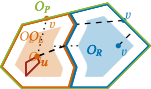
(c)

Figure 10: Visualization for the case distinction in the proof of Lemma 5.3: either (a) both points are in $S(O_{L})$ or $v$ is visited by either (b) $O_{R}$ or (c) a descendant of $O_{R}$. The dotted gray line represents a distance of at least $2r$, the dashed lines distances of at least $r$.

Let $G$ be a hyperbolic uniform disk graph with radius $r$. The vertices visited by generalized polygons of a valid and well-spaced polygon hierarchy form an independent set of $G$.

Proof.

Consider a valid and well-spaced polygon hierarchy. Let $O$ be a generalized polygon in this hierarchy and let $S(O)$ be the set of vertices of $G$ that are visited by $O$ or by descendants of $O$. We prove the following claim by induction.

Claim 1.

The vertices in $S(O)$ have pairwise distance $2r$ and each vertex in $S_{O}$ not visited by $O$ lies in the interior of $O$ and has distance at least $r$ from $O$.

Note that the first part of the claim that the vertices in $S(O)$ have pairwise distance $2r$ already implies the lemma statement when choosing $O$ to be the root of the hierarchy. The second part of the claim is only there to enable the induction over the tree structure. For the base case, $O$ is a leaf and $S(O)$ is exactly the set of vertices visited by $O$. Moreover, as the hierarchy is well-spaced, all vertices visited by $O$ have pairwise distance $2r$. Hence, the claim holds for leaves.

For the general case, let $O_{P}$ be a parent polygon with two children $O_{L}$ and $O_{R}$. To first get the simpler second part of the claim out of the way, let $v\in S(O_{P})$ be a vertex not visited by $O_{P}$. As the child–parent relation is valid, $v$ is either visited by $O_{L}$ and $O_{R}$ or by a descendant of one of the two. If $v$ is visited by $O_{L}$ and $O_{R}$ it lies in the interior of $O_{P}$ and has distance at least $r$ to $O_{P}$ as the child–parent relation is well-spaced. Otherwise, if $v$ is visited by neither $O_{L}$ nor $O_{R}$ but, without loss of generality, by a descendant of $O_{L}$. Then by induction, it lies in the interior of $O_{L}$ and has distance at least $r$ to $O_{L}$. As the interior of $O_{L}$ is a subset of the interior of $O_{P}$, the same holds for $O_{P}$.

It remains to show the first part of the claim, i.e., that any two vertices $u,v\in S(O_{P})$ have distance at least $2r$. If $u$ and $v$ are both visited by one of the polygons $O_{i}$ for $i\in\{P,L,R\}$, then this follows directly from the fact that the child–parent relation is well-spaced. Otherwise, assume without loss of generality that $u$ is not visited by one of these three polygons, but is instead visited by a descendant of $O_{L}$. We distinguish the following three cases of where $v$ lies; see also Figure 10. The first case is that $v$ is visited by $O_{L}$ or a descendant of $O_{L}$. The second case is that it is not visited by $O_{L}$ but by $O_{R}$ and the third case is that it is visited by neither $O_{L}$ nor $O_{R}$ but by a descendant of $O_{R}$. Clearly, this covers all possibilities.

In the first case, $v$ is also visited by $O_{L}$ or one if its descendants. Thus $u,v\in S(O_{L})$ and they have pairwise distance at least $2r$ by induction. In the second case, $v$ lies on $O_{R}$ but not on $O_{L}$ and thus in the exterior of $O_{L}$. As the hierarchy is well-spaced, $v$ has distance at least $r$ from $O_{L}$. Moreover, by induction, $u$ lies in the interior of $O_{L}$ and has distance at least $r$ from $O_{L}$. Thus, $u$ and $v$ have distance at least $2r$. For the third and final case, $v$ lies in the interior of $O_{R}$ and has distance at least $r$ from $O_{R}$ by induction. As the interiors of $O_{L}$ and $O_{R}$ are disjoint, the line segment between $u$ and $v$ has to cover the distance of at least $r$ from $u$ to $O_{L}$ and the distance of at least $r$ from $O_{R}$ to $v$. Thus, also in this final case, $u$ and $v$ have distance at least $2r$. ∎

5.4 Solving independent set

Lemma 5.3 tells us that for any hyperbolic uniform disk graph $G$, any valid and well-spaced polygon hierarchy yields an independent set. Moreover, by Corollary 5.3, we can obtain any independent set of $G$ from such a hierarchy. Thus, finding an independent set of size $k$ is equivalent to finding a valid and well-spaced polygon hierarchy that visit $k$ vertices of $G$. This can be done using a straightforward dynamic program on the set of all $k$-candidate nooses or, to be exact, on the not too large superset due to Lemma 5.3.

The dynamic program processes all $k$-candidate nooses in an order such that a noose $O$ is processed after a noose $O^{\prime}$ if the interior of $O^{\prime}$ is a subset of the interior of $O$. When processing a noose $O$, we compute a valid and well-spaced candidate noose hierarchy with root $O$ such that the number of vertices visited by nooses in the hierarchy is maximized. We call this the partial solution for $O$. Note that the maximum over the partial solutions of all nooses clearly yields a independent set with at least $k$ vertices if such an independent set exists. Also observe that when processing $O$, we have already computed the partial solutions of all possible child nooses of $O$ as we are only interested in valid hierarchies. Thus, to compute the partial solution for $O$, it suffices to consider all pairs of previously processed candidate nooses as potential children of $O$. For two such child candidates $O_{L}$ and $O_{R}$, we only need to check whether a child–parent relation with $O$ would be valid and well-spaced, which can be easily checked by only considering $O_{L}$ and $O_{R}$. Moreover, if this combination is valid, the number of vertices visited by the resulting hierarchy with $O$ as root is the sum of the partial solutions for $O_{L}$ and $O_{R}$ minus the vertices visited by $O_{L}$ and $O_{R}$. Finally, note that the start of the dynamic program is also easy, as each individual candidate noose by itself is a valid and well-spaced noose hierarchy (if all its visited vertices are sufficiently far apart). This concludes the description of the dynamic program. Note that the number of partial solutions and thus the running time increase excessively if $r$ is chosen sufficiently small depending on $n$. In this case, the algorithm is dominated by an algorithm for Euclidean intersection graphs. We obtain the following theorem.

See 3

Proof.

The three upper bounds for the running time follow via different algorithms. The first one, which depends on $r$, follows via the dynamic program described above. Here, we first enumerate all $k$-candidate nooses in $n^{\mathcal{O}(1+\frac{\log k}{r})}$ time (Lemma 5.3). Then, we determine partial solutions in the form of a polygon hierarchy for each $k$-candidate noose, by considering the partial solutions of all pairs of smaller polygons. In total, this means that the dynamic program can be evaluated in time cubic in the number of $k$-candidate nooses to find a valid and well-spaced polygon hierarchy maximizing the number of visited vertices in $n^{\mathcal{O}(1+\frac{\log k}{r})}$ time. As the vertices visited by a such a hierarchy form an independent set by Lemma 5.3 and the enumerated nooses admit a hierarchy corresponding to a size $k$ independent set in $G$ by Corollary 5.3 if such an independent set exists, this concludes the proof for the first algorithm.

At the same time Independent Set in $G\in\mathrm{HUDG}(r)$ can also be decided in $2^{\mathcal{O}(\sqrt{n})}$ time or $n^{\mathcal{O}(\sqrt{k})}$ time. To see this, recall that the uniformly sized hyperbolic disks representing the vertices of $G$ can also be viewed as Euclidean disks in the Poincaré disk. This means that $G$ is also an intersection graph of $n$ disks in the Euclidean plane. As shown by de Berg et al. [3, Corollary 2.4] and by Marx and Pilipczuk [37], Independent Set in a disk graph can be decided in $2^{\mathcal{O}(\sqrt{n})}$ time or $n^{\mathcal{O}(\sqrt{k})}$ time. ∎

6 Independent set approximation

Our approximation algorithm in Theorem 4 works similarly to Lipton and Tarjan’s version for planar graphs [33]: we repeatedly apply a separator until we get small patches and then solve each patch individually using the algorithm of Theorem 3. Unlike in planar graphs, we do not have a strong and readily available lower bound on the size of a maximum independent set to inform us how much of the graph we can afford to ignore, so we will start by proving one based on degeneracy.

A graph is said to be $k$-degenerate if every subgraph has a vertex of degree at most $k$. By picking this vertex $v$ and recursing on the subgraph with $v$ and its neighbors removed, we can always get an independent set of size at least $n/k$. Thus, this gives a lower bound on the size of a maximum independent set. We will use the following lemma to prove degeneracy.

For any hyperbolic uniform disk graph $G$, there is a vertex whose neighborhood can be covered with three cliques and stabbed with four points.

Proof.

Consider the disks of $G$ in the Poincaré disk model. For the remainder of the proof we will treat these as Euclidean disks that happen to get smaller as they get further from the origin. Take a disk $D$ with maximal distance to the origin and without loss of generality, assume its center $c$ lies on the negative part of the $y$-axis.

(a) Shrinking disks.

(b) Each wedge induces one clique.

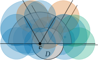
(c) A half-disk can be covered with four disks of half the radius.

Figure 11: Figures for the proof of Lemma 6.

Draw a horizontal line through $c$ and two lines at angle $\pi/3$ to form six wedges. The lower three wedges cannot contain any disk centers, because they would be further from the origin than $c$. Now, shrink each disk $D^{\prime}$ intersecting $D$ until it has the same radius as $D$, while keeping the point of $D^{\prime}$ closest to $c$ fixed; see Figure 11(a). The resulting disk will be a subset of $D^{\prime}$ and have its center in the same wedge. This makes the situation as in Figure 11(b) and means that we can use the same arguments as for unit disks [41]: for each wedge, the disks with center in that wedge that intersect $D$ must form a clique with $D$, giving three cliques in total.

Now, we will stab $D$ and the disks it intersects. For this, assume without loss of generality that $D$ has unit radius, then consider the problem of using unit disks to cover the upper half of a disk of radius $2$ centered at $c$. This can be done with four disks, as shown in Figure 11(c). The centers of these covering disks are our stabbing points: any disk $\overline{D}$ intersecting $D$ must have its center in the half-disk and thus $\overline{D}$ will be stabbed by the center of the covering disk that contains the center of $\overline{D}$. ∎

By repeatedly picking the vertex given by Lemma 6, the clique bound gives a simple 3-approximation algorithm for Independent Set. This generalizes the algorithm for unit disks by Marathe et al. [34]. Additionally, we get that any hyperbolic uniform disk graph is $(3\omega-3)$-degenerate with $\omega$ being the size of the largest clique. It is also $(4\ell-1)$-degenerate for ply $\ell$, so the maximum independent set has size $\Omega(n/\ell)$.

As first step in the approximation algorithm, we will use the separators of De Berg et al. [3] to separate the graph into many small patches. These separators are $36/37$-balanced, have size $\mathcal{O}(\sqrt{n})$, and can be found in $\mathcal{O}(n^{4})$ time. The following proof matches that of Frederickson [18] that is the main lemma for so-called $r$-divisions.

For any $t\geq 1$, we can in $\mathcal{O}(n^{4}\log(n/t))$ time partition $G$ into $\mathcal{O}(n/t)$ subgraphs of at most $t$ vertices each and $\mathcal{O}(n/\sqrt{t})$ cliques that separate the subgraphs from each other.

Proof.

We will iteratively apply a balanced clique-based separator until the size of the graph drops below $t$ vertices. Let $B(n,t)$ denote the number of cliques we need to remove from a graph of size $n$ and target size $t$. If $n\leq t$, nothing needs to be done, so $B(n,t)=0$. Otherwise, use the separator of De Berg et al. [3] to separate $G$ into two induced subgraphs of roughly equal size and recurse on these. Let $c$ be such that the number of cliques in the separator is always at most $c\sqrt{n}$. We will use induction to prove that $B(n,t)\leq 43cn/\sqrt{t}-7c\sqrt{n}$ for $n>t/37$. As base case we have $t/37<n\leq t$; here we established $B(n,t)=0$ and we have $\sqrt{37n/t}>1$, which implies $43cn/\sqrt{t}>7c\sqrt{n}$ so the bound holds. Now, for $n>t$ we get

$$B(n,t) \leq c\sqrt{n}+\max_{\alpha\in[\frac{1}{37},\frac{1}{2}]}B(\alpha n,t)+B((1-\alpha)n,t)$$

$$\leq c\sqrt{n}+43cn/\sqrt{t}-7c\sqrt{n}\cdot\left(\sqrt{1/37}+\sqrt{36/37}\right)$$

$$=43cn/\sqrt{t}-7c\sqrt{n}\cdot\left(\sqrt{1/37}+\sqrt{36/37}-1/7\right)$$

$$\leq 43cn/\sqrt{t}-7c\sqrt{n}.$$

Thus, $B(n,t)\in\mathcal{O}(n/\sqrt{t})$. The recursion has depth $\mathcal{O}(\log(n/t))$ and at each level we find separators in disjoint subgraphs of $G$. Thus, this procedure takes at most $\mathcal{O}(n^{4})$ time per level and $\mathcal{O}(n^{4}\log(n/t))$ time in total. ∎

This gives us all we need to prove Theorem 4. See 4

Proof.

Let $t=\ell^{2}/\varepsilon^{2}$ and apply Lemma 6, taking $\mathcal{O}(n^{4}\log n)$ time and removing $\mathcal{O}(\varepsilon n/\ell)$ cliques. Each of these cliques could only have contributed one point to the independent set. Since we know the maximum independent set has size $\Omega(n/\ell)$, we can only have thrown away a $\mathcal{O}(\varepsilon)$ fraction of it, so finding the exact maximum independent set in the remaining graph gives a $(1-\mathcal{O}(\varepsilon))$-approximation. We do this by applying Theorem 3 separately to each of the $\mathcal{O}(n/t)$ subgraphs of size $t$. This takes $t^{\mathcal{O}(1+\frac{\log t}{r})}=(\frac{\ell}{\varepsilon})^{\mathcal{O}(1+\frac{1}{r}\log\frac{\ell}{\varepsilon})}$ time for each subgraph and thus $n\cdot(\frac{\ell}{\varepsilon})^{\mathcal{O}(1+\frac{1}{r}\log\frac{\ell}{\varepsilon})}$ time in total. This makes the total running time $\mathcal{O}\left(n^{4}\log n\right)+n\cdot(\frac{\ell}{\varepsilon})^{\mathcal{O}(1+\frac{1}{r}\log\frac{\ell}{\varepsilon})}$ to find a $(1-\mathcal{O}(\varepsilon))$-approximation, so by appropriately adjusting $\varepsilon$ we can also get a $(1-\varepsilon)$-approximation with the same asymptotic running time. ∎

Using the results of Har-Peled [22], Theorem 4 also directly implies a similarly efficient approximation algorithm for Minimum Vertex Cover. A set $S$ of vertices in $G$ forms a vertex cover if every edge of $G$ is incident to some vertex of $S$. In the Minimum Vertex Cover problem we are given a graph $G$ and $\varepsilon>0$, and we wish to output that a vertex cover $S$ of $G$ that has size $(1+\varepsilon)k^{*}$, where $k^{*}$ is the size of the minimum vertex cover.

Let $\varepsilon\in(0,1)$ and let $G$ be a hyperbolic uniform disk graph with radius $r$ and ply $\ell$. Then a $(1+\varepsilon)$-approximate minimum vertex cover of $G$ can be computed in $\mathcal{O}\left(n^{4}\log n\right)+n\cdot(\frac{\ell}{\varepsilon})^{\mathcal{O}(1+\frac{1}{r}\log\frac{\ell}{\varepsilon})}$ time.

7 Algorithmic consequences of our separator

We can directly use our clique-based separator to compute independent sets and prove Corollary 1 via a simple divide-and conquer algorithm as in Corollary 2.4 of [3]. In our case, we use the trivial bound of $n$ on the size of the cliques in Theorem 1, which means that the weight of each clique in the separator is at most $\log(n+1)$. Consequently, the separator’s weight is at most $\mathcal{O}((1+1/r)\log^{2}n)$. The proof of Corollary 1 now follows that of Corollary 2.4 of [3], we merely replace the separator weight $\mathcal{O}(n^{1-1/d})$ with $\mathcal{O}((1+1/r)\log^{2}n)$. We give the proof for completeness.

See 1

Proof.

The algorithm works as follows: First, we find a balanced separator according to Theorem 1 in $\mathcal{O}(n\log n)$ time. We can then iterate over all possible intersections $X$ between a fixed optimum independent set and the separator. For every clique we can pick one of at most $n$ vertices, or nothing, so there are $(n+1)^{\mathcal{O}(1+1/r)\log n}=2^{\mathcal{O}(1+1/r)\log^{2}n}$ options. For each of these possible intersections, we remove all disks intersecting $X$, and recurse on both sides of the separator.

The running time follows the recursion $T(n)=2^{\mathcal{O}(1+1/r)\log^{2}n}T(\frac{2}{3}n)+n^{\mathcal{O}(1)}$. Denoting $2^{x}$ by $\exp_{2}(x)$, we can unroll this as follows:

$$T(n)=\exp_{2}\left(\mathcal{O}(1+1/r)\sum_{i=0}^{\log_{3/2}n}\log^{2}\left(\left(\frac{2}{3}\right)^{i}n\right)\right)=2^{\mathcal{O}(1+1/r)\log^{3}n}.$$

This concludes the proof. ∎

We note that the recursion added an extra logarithmic factor, which can be avoided via $\mathcal{P}$-flattened treewidth. We do not optimize this running time as the resulting algorithm would still be slower than that of Theorem 3. However, we do need to bound the $\mathcal{P}$-flattened treewidth for Corollary 1.

Consider a graph $G\in\mathrm{HUDG}(r)$ where $r\in\mathcal{O}(1)$, let $C$ be any clique of $G$, and let $s$ be the center of some disk of $C$. Then all other disk centers from $C$ are contained in a disk of radius $2r$ around $s$. Since $r\in\mathcal{O}(1)$, a disk of radius $r$ has area $\Theta(r^{2})$, and the above argument shows that the union of the disks in $C$ occupy area $\Theta(r^{2})$. We will now decompose $\mathbb{H}^{2}$ into regions of diameter at most $2r$ such that each region has an inscribed disk of radius at least $\Omega(r)$. The following can be derived from Lemma 2.1 (ii) of [28] and from Theorem 6 of [29].

[see [28, 29]] For any $\delta\in\mathcal{O}(1)$ there exists a subdivision of the hyperbolic plane into connected regions with the following properties:

1. Each region has diameter less than $\delta$ and thus area $\mathcal{O}(\delta^{2})$.

2. Each region has an inscribed disk of radius $\Omega(\delta)$, and thus area $\Omega(\delta^{2})$,

Moreover, the regions containing some given set of $n$ points can be computed in $\mathcal{O}(n)$ time.

We are now ready to prove Corollary 1. The proof merely needs to establish a clique partition $\mathcal{P}$ with a corresponding weighted treewidth bound, and the property that the graph $G_{\mathcal{P}}$ has maximum constant degree, that is, each clique of $\mathcal{P}$ has at most constantly many neighboring cliques. Then the machinery of [3] yields the desired algorithms automatically.

See 1

Proof.

Use the subdivision of Lemma 7 with $\delta=2r$. We can define a clique-partition $\mathcal{P}$ of $G$ by putting disks in the same partition class whenever their centers fall in the same region of the subdivision. Clearly each created class induces a clique in $G$ as the disk centers have pairwise distance less or equal to the diameter of the region, which is at most $2r$.

Fix such a clique partition $\mathcal{P}$, and consider now a separator from Theorem 1. If $X$ is one of the cliques in the separator, then let $p_{x}$ be the center of some disk of $X$. If $C\in\mathcal{P}$ and $X$ contain disks that intersect each other, then the graph distance of any pair of disks in $C$ and $X$ is at most $3$. Consequently, all disk centers in $C\cup X$ are covered by a disk $D$ of radius $3\cdot 2r=6r$ around $p_{x}$. Since each region of $\mathcal{P}$ has area $\Omega(r^{2})$, there can be at most $\mathcal{O}(1)$ regions of the subdivision contained inside $D$. In particular, $X$ can intersect at most $\mathcal{O}(1)$ cliques from $\mathcal{P}$.

Consider all cliques from $\mathcal{P}$ that are intersected by the separator cliques of Theorem 1: they clearly form a separator, and the above argument shows that there are $\mathcal{O}((1+1/r)\log n)$ such cliques in $\mathcal{P}$. Since each clique of $\mathcal{P}$ has weight at most $1+\log n$, we get a separator of weight $\mathcal{O}((1+1/r)\log^{2}n)$ over $\mathcal{P}$. Now [3] (see also [28]) implies that the $\mathcal{P}$-flattened treewidth of $G$ is $\mathcal{O}((1+1/r)\log^{2}n)$. Since $\mathcal{P}$ is a clique-partition with the additional property that each partition class is neighboring to $\mathcal{O}(1)$ other cliques, we can apply the entire machinery of [3] and derive the required algorithms. ∎

8 Conclusion

Summary.

In this article we have explored how the structure of hyperbolic uniform disk graphs depends on their radius $r$, and showed some algorithmic applications for the Independent Set problem. We proved a clique-based separator theorem, which showed that algorithms for the independent set of unit disks become more efficient as one increases the radius $r$ from the almost-Euclidean setting of $r=1/\sqrt{n}$ to $r=1$, while radii $r>1$ did not give any further gains on the separator size, but maintained a logarithmic separator. This result had some more or less immediate algorithmic consequences that we explored at the end of the paper.

After providing the separator for hyperbolic uniform disk graphs, we studied the Delaunay complexes of point sets that have pairwise distance at least $2r$, and uncovered further separator improvements as $r$ increases from $1$ to $\log n$. We used the outerplanarity bound of such Delaunay complexes to design an exact algorithm for Independent Set. The algorithm is based on dynamic programming using an unknown sphere cut decomposition of the solution’s Delaunay complex. The resulting running times became polynomial for $r\in\Omega(\log n)$

Finally, we used a separator-based subdivision together with our exact algorithm to give an approximation scheme for Independent Set for hyperbolic uniform disk graphs of a given ply, further extending our exact algorithm, with only quasi-polynomial dependence on $1/\varepsilon$ and the ply.

Future directions.

There are several intriguing future directions to explore in this space. First, is there a fully polynomial approximation scheme for Independent Set for $r\geq 1$? If not, is there at least an approximation scheme that is polynomial in $n$, quasi-polynomial in $1/\varepsilon$, but independent of the ply?

Second, it would be interesting to explore separators in higher-dimensional hyperbolic spaces. The only case studied there is $r=\Theta(1)$ [28]. One may expect that separator size should also decrease with growing $r$. Is there a constant $c_{d}$ such that Independent Set can be solved in polynomial time in $\mathbb{H}^{d}$ when $r\geq c_{d}\log n$?

Third, we should explore uniform disk graphs in surfaces of constant curvature, i.e., on the sphere, flat torus, and especially hyperbolic surfaces. What is the size of the best clique-based separator for a uniform disk graph of radius $r$ on a hyperbolic surface of genus $g$?

Fourth, it would be interesting to investigate the complexity of problems other than Independent Set, and study how their complexity scales with the radius of the disks, or equivalently, with the curvature of the underlying space.

Finally, it is unclear whether our bound on balanced separators is tight for all values of $r$. For constant $r$, regular hyperbolic tilings are hyperbolic uniform disk graphs with constant clique number and logarithmic treewidth, making our bound asymptotically tight. However, for larger radii, it could be possible to reduce the logarithmic factor.

References

- [1] Pankaj K. Agarwal, Marc J. Kreveld and Subhash Suri “Label placement by maximum independent set in rectangles” In Comput. Geom. 11.3-4, 1998, pp. 209–218 DOI: 10.1016/S0925-7721(98)00028-5
- [2] Brenda S. Baker “Approximation Algorithms for NP-Complete Problems on Planar Graphs” In J. ACM 41.1, 1994, pp. 153–180 DOI: 10.1145/174644.174650
- [3] Mark Berg, Hans L. Bodlaender, Sándor Kisfaludi-Bak, Dániel Marx and Tom C. Zanden “A Framework for Exponential-Time-Hypothesis-Tight Algorithms and Lower Bounds in Geometric Intersection Graphs” In SIAM J. Comput. 49.6, 2020, pp. 1291–1331 DOI: 10.1137/20M1320870
- [4] Mark Berg, Sándor Kisfaludi-Bak, Morteza Monemizadeh and Leonidas Theocharous “Clique-Based Separators for Geometric Intersection Graphs” In Algorithmica 85.6, 2023, pp. 1652–1678 DOI: 10.1007/S00453-022-01041-8
- [5] Nicholas Bieker, Thomas Bläsius, Emil Dohse and Paul Jungeblut “Recognizing Unit Disk Graphs in Hyperbolic Geometry is -Complete” In CoRR abs/2301.05550, 2023 DOI: 10.48550/ARXIV.2301.05550
- [6] Thomas Bläsius, Philipp Fischbeck, Tobias Friedrich and Maximilian Katzmann “Solving Vertex Cover in Polynomial Time on Hyperbolic Random Graphs” In Theory Comput. Syst. 67.1, 2023, pp. 28–51 DOI: 10.1007/S00224-021-10062-9
- [7] Thomas Bläsius, Cedric Freiberger, Tobias Friedrich, Maximilian Katzmann, Felix Montenegro-Retana and Marianne Thieffry “Efficient Shortest Paths in Scale-Free Networks with Underlying Hyperbolic Geometry” In ACM Transactions on Algorithms (TALG) 18.2, 2022, pp. 19:1–19:32 DOI: 10.1145/3516483
- [8] Thomas Bläsius, Tobias Friedrich and Maximilian Katzmann “Efficiently Approximating Vertex Cover on Scale-Free Networks with Underlying Hyperbolic Geometry” In Algorithmica 85.12, 2023, pp. 3487–3520 DOI: 10.1007/S00453-023-01143-X
- [9] Thomas Bläsius, Tobias Friedrich, Maximilian Katzmann and Daniel Stephan “Strongly Hyperbolic Unit Disk Graphs” In 40th International Symposium on Theoretical Aspects of Computer Science, STACS 254, LIPIcs, 2023, pp. 13:1–13:17 DOI: 10.4230/LIPICS.STACS.2023.13
- [10] Thomas Bläsius, Tobias Friedrich and Anton Krohmer “Hyperbolic Random Graphs: Separators and Treewidth” In 24th Annual European Symposium on Algorithms, ESA 57, LIPIcs, 2016, pp. 15:1–15:16 DOI: 10.4230/LIPICS.ESA.2016.15
- [11] Hans L. Bodlaender “A Partial k-Arboretum of Graphs with Bounded Treewidth” In Theor. Comput. Sci. 209.1-2, 1998, pp. 1–45 DOI: 10.1016/S0304-3975(97)00228-4
- [12] Vincent Bouchitté, Frédéric Mazoit and Ioan Todinca “Chordal embeddings of planar graphs” In Discret. Math. 273.1-3, 2003, pp. 85–102 DOI: 10.1016/S0012-365X(03)00230-9
- [13] Karl Bringmann, Sándor Kisfaludi-Bak, Michal Pilipczuk and Erik Jan Leeuwen “On Geometric Set Cover for Orthants” In 27th Annual European Symposium on Algorithms, ESA 144, LIPIcs, 2019, pp. 26:1–26:18 DOI: 10.4230/LIPICS.ESA.2019.26
- [14] Timothy M. Chan “Polynomial-time approximation schemes for packing and piercing fat objects” In J. Algorithms 46.2, 2003, pp. 178–189 DOI: 10.1016/S0196-6774(02)00294-8
- [15] Marek Cygan, Fedor V Fomin, Łukasz Kowalik, Daniel Lokshtanov, Dániel Marx, Marcin Pilipczuk, Michał Pilipczuk and Saket Saurabh “Parameterized Algorithms” Springer, 2015
- [16] Frederic Dorn, Eelko Penninkx, Hans L. Bodlaender and Fedor V. Fomin “Efficient Exact Algorithms on Planar Graphs: Exploiting Sphere Cut Decompositions” In Algorithmica 58.3, 2010, pp. 790–810 DOI: 10.1007/s00453-009-9296-1
- [17] Frank Eijkhof, Hans L. Bodlaender and Arie M… Koster “Safe Reduction Rules for Weighted Treewidth” In Algorithmica 47.2, 2007, pp. 139–158 DOI: 10.1007/S00453-006-1226-X
- [18] Greg N. Frederickson “Fast Algorithms for Shortest Paths in Planar Graphs, with Applications” In SIAM J. Comput. 16.6, 1987, pp. 1004–1022 DOI: 10.1137/0216064
- [19] Tobias Friedrich and Anton Krohmer “On the Diameter of Hyperbolic Random Graphs” In SIAM Journal on Discrete Mathematics 32.2, 2018, pp. 1314–1334 DOI: 10.1137/17M1123961
- [20] Marvin Jay Greenberg “Euclidean and Non-Euclidean Geometries: Development and History” W. H. FreemanCompany, 1993
- [21] Luca Gugelmann, Konstantinos Panagiotou and Ueli Peter “Random Hyperbolic Graphs: Degree Sequence and Clustering” In 39th International Colloquium on Automata, Languages, and Programming (ICALP), 2012, pp. 573–585 DOI: 10.1007/978-3-642-31585-5_51
- [22] Sariel Har-Peled “Approximately: Independence Implies Vertex Cover” In CoRR abs/2308.00840, 2023 DOI: 10.48550/ARXIV.2308.00840
- [23] Sariel Har-Peled “Quasi-Polynomial Time Approximation Scheme for Sparse Subsets of Polygons” In 30th Annual Symposium on Computational Geometry, SoCG ACM, 2014, pp. 120 DOI: 10.1145/2582112.2582157
- [24] Dorit S. Hochbaum and Wolfgang Maass “Approximation Schemes for Covering and Packing Problems in Image Processing and VLSI” In J. ACM 32.1, 1985, pp. 130–136 DOI: 10.1145/2455.214106
- [25] Russell Impagliazzo and Ramamohan Paturi “On the Complexity of -SAT” In Journal of Computer and System Sciences 62.2, 2001, pp. 367–375 DOI: 10.1006/jcss.2000.1727
- [26] Shreesh Jadhav and Asish Mukhopadhyay “Computing a Centerpoint of a Finite Planar Set of Points in Linear Time” In Discret. Comput. Geom. 12, 1994, pp. 291–312 DOI: 10.1007/BF02574382
- [27] Sándor Kisfaludi-Bak “A quasi-polynomial algorithm for well-spaced hyperbolic TSP” In J. Comput. Geom. 12.2, 2021, pp. 25–54 DOI: 10.20382/JOCG.V12I2A3
- [28] Sándor Kisfaludi-Bak “Hyperbolic intersection graphs and (quasi)-polynomial time” In Proceedings of the 2020 ACM-SIAM Symposium on Discrete Algorithms, SODA SIAM, 2020, pp. 1621–1638 DOI: 10.1137/1.9781611975994.100
- [29] Sándor Kisfaludi-Bak and Geert Wordragen “A Quadtree, a Steiner Spanner, and Approximate Nearest Neighbours in Hyperbolic Space” In 40th International Symposium on Computational Geometry, SoCG 293, LIPIcs, 2024, pp. 68:1–68:15 DOI: 10.4230/LIPICS.SOCG.2024.68
- [30] Paul Koebe “Kontaktprobleme der konformen Abbildung” Hirzel, 1936
- [31] Dmitri Krioukov, Fragkiskos Papadopoulos, Maksim Kitsak, Amin Vahdat and Marián Boguñá “Hyperbolic Geometry of Complex Networks” In Phys. Rev. E 82 American Physical Society, 2010, pp. 036106 DOI: 10.1103/PhysRevE.82.036106
- [32] Richard J. Lipton and Robert Endre Tarjan “A separator theorem for planar graphs” In SIAM Journal on Applied Mathematics 36.2, 1979, pp. 177–189
- [33] Richard J. Lipton and Robert Endre Tarjan “Applications of a planar separator theorem” In SIAM Journal on Computing 9.3, 1980, pp. 615–627
- [34] Madhav V. Marathe, H. Breu, Harry B. III, S.. Ravi and Daniel J. Rosenkrantz “Simple heuristics for unit disk graphs” In Networks 25.2, 1995, pp. 59–68 DOI: 10.1002/NET.3230250205
- [35] Dániel Marx “On the Optimality of Planar and Geometric Approximation Schemes” In 48th Annual IEEE Symposium on Foundations of Computer Science (FOCS 2007) IEEE Computer Society, 2007, pp. 338–348 DOI: 10.1109/FOCS.2007.26
- [36] Dániel Marx, Marcin Pilipczuk and Michal Pilipczuk “On Subexponential Parameterized Algorithms for Steiner Tree and Directed Subset TSP on Planar Graphs” In 59th IEEE Annual Symposium on Foundations of Computer Science, FOCS IEEE Computer Society, 2018, pp. 474–484 DOI: 10.1109/FOCS.2018.00052
- [37] Dániel Marx and Michal Pilipczuk “Optimal Parameterized Algorithms for Planar Facility Location Problems Using Voronoi Diagrams” In ACM Trans. Algorithms 18.2, 2022, pp. 13:1–13:64 DOI: 10.1145/3483425
- [38] Colin McDiarmid and Tobias Müller “Integer realizations of disk and segment graphs” In J. Comb. Theory B 103.1, 2013, pp. 114–143 DOI: 10.1016/J.JCTB.2012.09.004
- [39] Gary L. Miller, Shang-Hua Teng, William P. Thurston and Stephen A. Vavasis “Separators for sphere-packings and nearest neighbor graphs” In Journal of the ACM 44.1, 1997, pp. 1–29 DOI: 10.1145/256292.256294
- [40] Tobias Müller and Merlijn Staps “The Diameter of KPKVB Random Graphs” In Advances in Applied Probability 51.2 Applied Probability Trust, 2019, pp. 358–377 DOI: 10.1017/apr.2019.23
- [41] M.J.P. Peeters “On coloring j-unit sphere graphs” Pagination: 6, vi FEW 512, Research memorandum / Tilburg University, Department of Economics, 1991
- [42] Neil Robertson and P. Seymour “Graph minors. X. Obstructions to tree-decomposition” In Journal of Combinatorial Theory, Series B 52.2, 1991, pp. 153–190 DOI: 10.1016/0095-8956(91)90061-N
- [43] Paul D. Seymour and Robin Thomas “Call Routing and the Ratcatcher” In Comb. 14.2, 1994, pp. 217–241 DOI: 10.1007/BF01215352