Orthonormal and periodic levels for Quantum Cascade Laser simulation

Abstract

A Python package to evaluate Wannier, Wannier-Stark, and EZ (both Energy and location Z resolved) levels for Quantum Cascade Lasers is presented. We provide the underlying theory in detail with a focus on the orthonormality and periodicity of the generated states.

I Introduction

The operation of Quantum Cascade Lasers (QCLs)[1, 2, 3] is based on optical transitions between quantized levels in the conduction band of a semiconductor heterostructure. Further such levels are employed for an effective population of the upper laser level and the emptying of the lower laser level, which is facilitated by a sequence of tunneling and scattering processes at the designated bias. In order to provide light amplification over a larger spatial range, a carefully designed sequence of layers, referred to as module in the following, is repeated periodically about 30-300 times. Each of these modules contains a laser transition, so that the electron flow resembles a cascade.

The design of QCLs requires reliable simulation schemes, see Refs. 4, 5 for an overview. In a first step this needs to establish the energy levels for a given sequence of semiconductor layers. Here the periodic repetition of the module is typically reflected by the requirement that the levels in a given module are periodically repeated in the neighboring modules (periodicity criterion). Alternatively, few modules embedded between contacts can be simulated[6]. Furthermore, the orthonormality of the levels is highly relevant, as this is a common requirement for basis states and often tacitly assumed in concepts such as Fermi’s golden rule.

The periodicity criterion and orthonormality are actually difficult to achieve simultaneously. The reason is that common approaches require boundary conditions to avoid escape to infinity. In this case, levels located in different modules do not satisfy the periodicity criterion, as their distance to the boundary differs. Alternatively, a central module is identified and levels in neighboring modules are defined by shifting the levels from the central module. In this case, levels in neighboring modules are solutions of a setup with shifted boundaries and thus intermodule orthogonality is not guaranteed. Albeit these orthogonality violations may be small[7] they constitute a matter of concern.

A second issue affecting the orthogonality of levels is the common use of energy-dependent effective masses, see, e.g., Refs. 6, 8, 9. These are particular important for infrared QCLs with level energies of several 100 meV above the conduction band edge where the conduction band becomes non-parabolic, see e.g. Ref. 10 and references cited therein. If the Hamiltonian contains energy-dependent components, the solutions obtained at different energies are not orthogonal.

Over the last decades our group developed simulation techniques for QCLs, where we strived to overcome the issues mentioned above. From the very start we used a basis of Wannier states[11] to combine the periodicity condition with orthogonality. Later, we implemented non-parabolicity [12] by applying a two-band model [13, 14, 15] explicitly. In this article we give a comprehensive discussion of the underlying concepts. We also carefully overhauled our codes and provide a new Python-based simulation package resource_QCL to generate sets of orthonormal and periodic levels for a variety of QCL simulations. The package is provided in the supplemental material and can be used under a CC-BY license.

II Generating Wannier states

To avoid boundary conditions, which are incompatible with the periodicity condition, we start by calculating Bloch functions for an infinite periodic repetition of the modules without bias. These are mapped on Wannier functions $w^{\nu n}$ by a unitary transformation. Here, $n$ specifies the module to which they are localized and $\nu$ distinguishes different levels in a module. Most importantly, they satisfy the periodicity criterion and constitute a basis, which is complete within the energy range covered by the Bloch bands considered. In particular, we obtain an explicit matrix representation (18) of the Hamiltonian for the heterostructure. Fig. 1 shows an example for these Wannier levels. Here, we consider the sample of Ref. 16, which achieved room-temperature CW operation by double-phonon extraction using two extraction levels with a spacing of the optical phonon energy.

Nonparabolicity is treated by a two-band model and keeping both the conduction and valence band components $(w^{\nu n}_{c}(z),w^{\nu n}_{v}(z))^{\textrm{tr}}$. Thus orthonormality is ensured, see Eq. (17) below. This task is performed by the routine resource_QCL.calcWannier1 which establishes the relevant data based on the following physical input parameters:

thlist

list of layer thicknesses $w_{i}$ in one module

Eclist

list of conduction band offsets $V_{i}$ for the layers

mclist

list of effective masses $m_{c}^{*}$ at the $\Gamma$ point

E_Kane

the common Kane energy $E_{\textrm{Kane}}$

In this section the underlying theory and numerical issues are detailed.

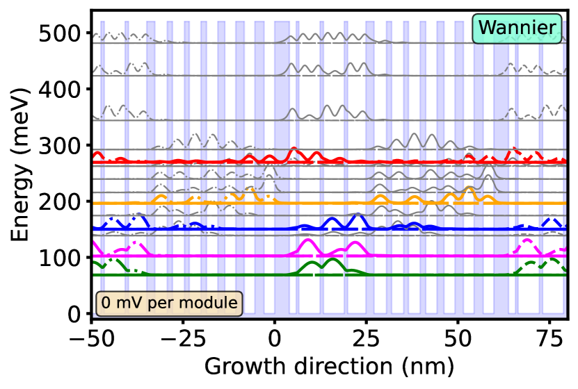
Figure 1: Wannier states for the QCL of Ref. 16. The band gap is depicted by the grey/blue area. The lines show the probability density $w^{\nu,n}_{c}(z)^{2}+w^{\nu,n}_{v}(z)^{2}$ for the 14 lowest Wannier states (label $\nu$), where the baseline is shifted by the respective level energy. Thick colored lines indicate levels related to (from top to bottom) the upper laser, the injector, the lower laser, and the two extraction levels. Full lines refer to levels in the central module ($n=0$) ranging from 0 to 59.8 nm. Dashed and dot-dashed lines are periodic repetitions to the right and left module ($n=\pm 1$), respectively.

II.1 Two-band formalism

The two-band model considers states $(\Psi_{c}(z),\Psi_{v}(z))^{\textrm{tr}}$, which contain a conduction and valence band contribution in order to include non-parabolicity in the conduction band for planar systems. This model is applicable only along a single spatial direction, typically the growth direction denoted as $z$. In the absence of an external potential, the two-band Hamiltonian is given by the matrix [13]

$$\hat{H}^{\textrm{het}}=\begin{pmatrix}E_{c}(z)&\frac{p_{cv}}{m_{e}}\frac{\hbar}{{\rm i}}\frac{\partial}{\partial z}\\ \frac{p_{vc}}{m_{e}}\frac{\hbar}{{\rm i}}\frac{\partial}{\partial z}&E_{v}(z)\end{pmatrix}\,.$$ (1)

$E_{c}(z)$ is the conduction-band offset, which depends on the specific material at position $z$. Correspondingly, $E_{v}(z)$ mimics the valence band offset. The stationary Schrödinger equation reads

$$\hat{H}^{\textrm{het}}\begin{pmatrix}\Psi_{c}(z)\\ \Psi_{v}(z)\end{pmatrix}=E\begin{pmatrix}\Psi_{c}(z)\\ \Psi_{v}(z)\end{pmatrix}$$ (2)

where the lower component provides

$$\Psi_{v}(z)=\frac{1}{E-E_{v}(z)}\frac{p_{vc}}{m_{e}}\frac{\hbar}{{\rm i}}\frac{\partial\Psi_{c}(z)}{\partial z}\,.$$ (3)

Inserting into the upper component gives the Schrödinger-like equation

$$\left[E_{c}(z)-\frac{\partial}{\partial z}\frac{\hbar^{2}}{2m_{c}(E,z)}\frac{\partial}{\partial z}\right]\Psi_{c}(z)=E\Psi_{c}(z)$$ (4)

with the energy-dependent mass

$$m_{c}(E,z)=\frac{m_{e}^{2}[E-E_{v}(z)]}{2|p_{cv}|^{2}}\,,$$ (5)

which also depends on the material at position $z$. Identifying the known effective mass $m^{*}_{c}$ at the $\Gamma$ point as $m_{c}(E_{c})$, we find the relation

$$m^{*}_{c}(z)=\frac{m_{e}^{2}(E_{c}(z)-E_{v}(z))}{2|p_{cv}|^{2}}$$

so that the values of $E_{c}(z),E_{v}(z),p_{cv}$ and $m^{*}_{c}(z)$ are intrinsically related to each other within the two-band model. The value of $p_{cv}$ is required to be the same for all materials involved in a given heterostructure within the two band model. Its value is provided by the Kane energy[15] $E_{\textrm{Kane}}=2|p_{vc}|^{2}/m_{e}$, which is used as an input parameter. Focusing on the conduction band, we use literature values for $m^{*}_{c}(z)$ and $E_{c}(z)$ for the respective material at $z$ as further input parameters. Hence we apply

$$E_{v}(z)=E_{c}(z)-2|p_{vc}|^{2}\frac{m^{*}_{c}(z)}{m_{e}^{2}}=E_{c}(z)-E_{\textrm{Kane}}\frac{m^{*}_{c}(z)}{m_{e}}\,,$$ (6)

for the effective valence band offset. This approximation deviates from the actual material value, as expected within the framework of the two-band model, which simplifies the intricate multi-band structure of the valence band. Here, its sole purpose is to quantify the energy-dependent effective mass $m_{c}(E,z)$ from Eq. (5). Finally, the phase of the momentum matrix elements is chosen as

$$p_{vc}={\rm i}|p_{vc}|={\rm i}\sqrt{\frac{m_{e}E_{\textrm{Kane}}}{2}}\textrm{ and consequently }p_{cv}=-{\rm i}|p_{vc}|\,,$$

which provides a real Hamiltonian (1) and consequently the option to establish real Wannier functions below.

Note, that the solutions $\Psi^{n}_{c}(z)$ of the effective Schrödinger equation (4) at different eigenenergies $E_{n}$ are not necessarily orthogonal due to the energy-dependent mass. However, adding the valence band component from Eq. (3) provides after normalization

$$\int{\rm d}z\,\left[\Psi^{m*}_{c}(z)\Psi^{n}_{c}(z)+\Psi^{m*}_{v}(z)\Psi^{n}_{v}(z)\right]=\delta_{mn}$$

as they are actually solutions of the energy-independent Hamiltonian (1). The main concept in the following is to start with othonormal Wannier functions, see Eq. (17), and inherit this property to other sets by unitary transformations.

II.2 Bloch States

Now we consider a QCL, where each module consists of a sequence of $N$ layers with thicknesses $w_{0},w_{1},\ldots w_{N-1}$ extending from $z_{i}$ to $z_{i+1}=z_{i}+w_{i}$. Here we set $z_{0}=0$ and denote $z_{N}=d$. As the modules are periodically repeated, we have a periodic structure with period $d=\sum_{i=0}^{N-1}w_{i}$. Consequently, for vanishing external potential, the eigenstates are Bloch states $(\Psi^{q\nu}_{c}(z),\Psi^{q\nu}_{v}(z))^{\textrm{tr}}$ as characterized by the Bloch vector $q$ (with $-\pi/d<q\leq\pi/d$ covering the one-dimensional Brillouin zone) and the band index $\nu$. The Bloch condition reads

$$\begin{pmatrix}\Psi^{q\nu}_{c}(z+d)\\ \Psi^{q\nu}_{v}(z+d)\end{pmatrix}={\rm e}^{{\rm i}qd}\begin{pmatrix}\Psi^{q\nu}_{c}(z)\\ \Psi^{q\nu}_{v}(z)\end{pmatrix}$$ (7)

for all $z$. In order to calculate the Bloch states we note that in a region $z_{i}<z<z_{i+1}$ of constant $E_{c}(z)=V_{i}$ and constant $m_{c}(E,z)=m_{i}(E)$, Eq. (4) is solved by

$$\begin{split}&\Psi^{i}_{c}(z)=C_{i}\cos\left[k_{i}\left(z-z_{i}-\frac{w_{i}}{2}\right)\right]+\frac{D_{i}}{k_{i}}\sin\left[k_{i}\left(z-z_{i}-\frac{w_{i}}{2}\right)\right]\\ &\textrm{with }k_{i}=\frac{\sqrt{2m_{i}(E)(E-V_{i})}}{\hbar}\quad\textrm{for }z_{i}<z<z_{i+1}\end{split}$$ (8)

This provides a finite nonvanishing result for the $D_{i}$-term at $k_{i}=0$, where we implement $\frac{1}{k_{i}}\sin(k_{i}z)=z\;\textrm{sinc}(k_{i}z/\pi)$ with the normalized sinc function $\textrm{sinc}(x)=\sin(\pi x)/(\pi x)$ as defined in the NumPy library of Python.

For $E<V_{i}$, $k_{i}={\rm i}\lambda_{i}$ is purely imaginary and we get the equivalent representation

$$\begin{split}&\Psi^{i}_{c}(z)=C_{i}\cosh\left[\lambda_{i}\left(z-z_{i}-\frac{w_{i}}{2}\right)\right]+\frac{D_{i}}{\lambda_{i}}\sinh\left[\lambda_{i}\left(z-z_{i}-\frac{w_{i}}{2}\right)\right]\\ &\textrm{with }\lambda_{i}=\frac{\sqrt{2m_{i}(E)(V_{i}-E)}}{\hbar}\end{split}$$

Our choice for the middle point of the layers $z_{i}+\frac{w_{i}}{2}$ as reference position limits the exponential growth of the hyperbolic functions, which reduces numerical instabilities.

At the boundary $z_{n+1}$ between two layers, the functions $\Psi_{c}(z)$ and $\Psi_{v}(z)$ should be continuous. From Eq. (3) we find, that this is equivalent to the two equations

$$\begin{split}\Psi^{n}_{c}(z_{n+1}-0^{+})&=\Psi^{n+1}_{c}(z_{n+1}+0^{+})\\ \frac{1}{m_{n}}\frac{\partial\Psi^{n}_{c}(z)}{\partial z}_{|z=z_{n+1}-0^{+}}&=\frac{1}{m_{n+1}}\frac{\partial\Psi^{n+1}_{c}(z)}{\partial z}_{|z=z_{n+1}+0^{+}}\,,\end{split}$$

where $0^{+}$ stands for an infinitesimal positive quantity (more formally to be replaced by an $\epsilon>0$ with $\lim_{\epsilon\to 0}$). Inserting Eq. (8) provides the relation

$$\begin{split}&\begin{pmatrix}C_{n+1}\\ D_{n+1}\end{pmatrix}=\tilde{\cal M}_{n}\begin{pmatrix}C_{n}\\ D_{n}\end{pmatrix}\quad\textrm{with }\tilde{\cal M}_{n}=\begin{pmatrix}c_{n}c_{n+1}-\beta_{n}k_{n}^{2}s_{n}s_{n+1}&s_{n}c_{n+1}+\beta_{n}c_{n}s_{n+1}\\ -c_{n}s_{n+1}k_{n+1}^{2}-\beta_{n}k_{n}^{2}s_{n}c_{n+1}&-k_{n+1}^{2}s_{n}s_{n+1}+\beta_{n}c_{n}c_{n+1}\end{pmatrix}\\ &\textrm{where}\quad\beta_{n}=\frac{m_{n+1}}{m_{n}}\qquad c_{n}=\cos\left(\frac{k_{n}w_{n}}{2}\right)\qquad s_{n}=\frac{1}{k_{n}}\sin\left(\frac{k_{n}w_{n}}{2}\right)=\frac{w_{n}}{2}\textrm{sinc}\left(\frac{k_{n}w_{n}}{2\pi}\right)\end{split}$$

Here the values $c_{n}$ and $s_{n}$ are real both for real and (purely) imaginary $k_{n}$, so that the entire matrix is real. Note that the matrices $\tilde{\cal M}_{n}$ depend on $E$ via $k_{n}$ and $m_{n}$. Applying the Bloch condition (7) for the conduction band component $\Psi^{q\nu}_{c}(z+d)={\rm e}^{{\rm i}qd}\Psi^{q\nu}_{c}(z)$ for $z_{0}\leq z<z_{1}$, where $z_{N}\leq z+d<z_{N+1}$ is in region $N$, which has the same properties as region 0 (i.e. $m_{N}=m_{0}$ and $V_{N}=V_{0}$) requires

$${\rm e}^{{\rm i}qd}\begin{pmatrix}C_{0}\\ D_{0}\end{pmatrix}=\begin{pmatrix}C_{N}\\ D_{N}\end{pmatrix}=\tilde{\cal M}\begin{pmatrix}C_{0}\\ D_{0}\end{pmatrix}$$ (9)

with $\tilde{\cal M}=\tilde{\cal M}_{N-1}\tilde{\cal M}_{N-2}\ldots\tilde{\cal M}_{1}\tilde{\cal M}_{0}$. This only allows for non-vanishing $C_{0},D_{0}$ if $\textrm{det}\{\tilde{\cal M}-{\rm e}^{{\rm i}qd}{\cal I}\}=0$. As $\tilde{\cal M}$ depends on energy this provides a set of energies $E_{\nu}(q)$ with $\nu=1,2,\ldots$ for each value of $q$. (Restricting to conduction band states, we consider only solutions, where $E$ is larger than the minimal value of the set $\{V_{n}\}$.)

Straightforward evaluation provides det$\{\tilde{\cal M}_{n}\}=\beta_{n}$. Thus det$\{\tilde{\cal M}\}=m_{N}/m_{0}=1$ due to the periodicity. This provides

$$\begin{split}0=&\textrm{det}\{\tilde{\cal M}-{\rm e}^{{\rm i}qd}{\cal I}\}=1-(M_{00}+M_{11}){\rm e}^{{\rm i}qd}+{\rm e}^{2{\rm i}qd}\\ =&{\rm e}^{{\rm i}qd}\left[2\cos(qd)-(M_{00}+M_{11})\right]\\ \Leftrightarrow&M_{00}+M_{11}=2\cos(qd)\end{split}$$

For the specific energies $E_{\nu}(q)$, a solutions of Eq. (9) is given by

$$\begin{pmatrix}C_{0}\\ D_{0}\end{pmatrix}=\begin{pmatrix}\tilde{M}_{11}-{\rm e}^{{\rm i}qd}\\ -\tilde{M}_{10}\end{pmatrix}+0.5\begin{pmatrix}-\tilde{M}_{01}\\ \tilde{M}_{00}-{\rm e}^{{\rm i}qd}\end{pmatrix}$$ (10)

where we added solutions for the first and second row in order to avoid problems with accidental small values. Furthermore, we directly get all coefficients

$$\begin{pmatrix}C_{n}\\ D_{n}\end{pmatrix}=\tilde{\cal M}_{n-1}\tilde{\cal M}_{n-2}\ldots\tilde{\cal M}_{0}\begin{pmatrix}C_{0}\\ D_{0}\end{pmatrix}$$

which allows us to construct the wave function $\Psi^{n}_{c}(z)$ for arbitrary $z$ in the interval $0<z\leq d$ by evaluation of Eq. (8) in the appropriate region. [Outside this central module, the periodicity condition (7) is applied to evaluate $\Psi^{n}_{c}(z)$ based on the result in the central module.] Furthermore, $\Psi^{n}_{v}(z)$ is obtained from Eq. (3). By rescaling $C_{0}^{\nu}(q)$ and $D_{0}^{\nu}(q)$ the normalization

$$\int_{0}^{d}{\rm d}z\left[|\Psi^{\nu q}_{c}(z)|^{2}+|\Psi^{\nu q}_{v}(z)|^{2}\right]=1$$ (11)

is achieved. This procedure defines the initial Bloch functions. As the Hamiltonian is real we have $E_{\nu}(-q)=E_{\nu}(q)$ and our choice (10) guarantees $C_{n}(-q)=C_{n}(q)^{*}$ and = $D_{n}(-q)=D_{n}(q)^{*}$ so that

$$\begin{pmatrix}\Psi^{q\nu}_{c}(z)\\ \Psi^{q\nu}_{v}(z)\end{pmatrix}^{*}=\begin{pmatrix}\Psi^{-q\nu}_{c}(z)\\ \Psi^{-q\nu}_{v}(z)\end{pmatrix}$$ (12)

Furthermore, the chosen Bloch funtions are periodic in $q$ and continuous at $q=\pm\pi/d$.

In practice, we calculate the Bloch functions for a finite number $(N_{q})$ of $q$-values

$$q_{j}=-\frac{\pi}{d}-\frac{\pi}{N_{q}d}+\frac{2\pi}{N_{q}d}j\quad\textrm{for }j=1,2,\ldots N_{q}\,,$$ (13)

which are chosen such that they cover the entire Brillouin zone with equal spacing. Furthermore for each $j$, we have a value $k=N_{q}+1-j$, so that both $q_{j}$ and $q_{k}=-q_{j}$ are in the set of chosen $q$-values. The choice of $q_{j}$ values restricts to the eigenstates of a system of length $L=N_{q}d$ with boundary conditions $\Psi(x+L)=(-1)^{(N_{q}+1)}\Psi(x)$. (For odd $N_{q}$ this is the standard Born von-Karman boundary condition). Thus, the eigenstates are orthogonal. Based on normalization for a single period before, we thus find

$$\int_{L/2}^{L/2}{\rm d}z\,\begin{pmatrix}\Psi^{q_{j}\nu}_{c}(z)&\Psi^{q_{j}\nu}_{v}(z)\end{pmatrix}^{*}\begin{pmatrix}\Psi^{q_{k}\mu}_{c}(z)\\ \Psi^{q_{k}\mu}_{v}(z)\end{pmatrix}=N_{q}\delta_{\nu\mu}\delta_{jk}$$ (14)

As the Bloch states are eigenstates of the Hamiltonian $\hat{H}^{\textrm{het}}$ for the ideal layer sequence (1), we can write its matrix elements of

$$\int_{L/2}^{L/2}{\rm d}z\,\begin{pmatrix}\Psi^{q_{j}\nu}_{c}(z)&\Psi^{q_{j}\nu}_{v}(z)\end{pmatrix}^{*}\hat{H}^{\textrm{het}}\begin{pmatrix}\Psi^{q_{k}\mu}_{c}(z)\\ \Psi^{q_{k}\mu}_{v}(z)\end{pmatrix}\\ =E_{\nu}(q)N_{q}\delta_{\nu\mu}\delta_{jk}$$ (15)

In the continuum limit $L=N_{q}d\to\infty$, one needs to replace $N_{q}\delta_{jk}\to 2\pi\delta(q_{j}-q_{k})$ at the right-hand of Eqs. (14,15).

II.3 Wannier States

The Wannier functions are given by

$$\begin{split}\begin{pmatrix}w_{c}^{\nu,n}(z)\\ w_{v}^{\nu,n}(z)\end{pmatrix}=&\frac{d}{2\pi}\int_{-\pi/d}^{\pi/d}{\rm d}q\,{\rm e}^{-{\rm i}qnd}\begin{pmatrix}\Psi^{q\nu}_{c}(z)\\ \Psi^{q\nu}_{v}(z)\end{pmatrix}\\ \approx&\frac{1}{N_{q}}\sum_{q}{\rm e}^{-{\rm i}qnd}\begin{pmatrix}\Psi^{q\nu}_{c}(z)\\ \Psi^{q\nu}_{v}(z)\end{pmatrix}\end{split}$$ (16)

and satisfy $w^{\nu,n}(z)=w^{\nu,0}(z-nd)$, so that it is sufficient to calculate the $n=0$ terms. Here the $q$ sum runs over the values specified in Eq. (13). For the normalization (11) they satisfy

$$\int{\rm d}z\begin{pmatrix}w_{c}^{\nu,n}(z)&w_{v}^{\nu,n}(z)\end{pmatrix}\begin{pmatrix}w_{c}^{\mu,m}(z)\\ w_{v}^{\mu,m}(z)\end{pmatrix}=\delta_{nm}\delta_{\nu\mu}$$ (17)

as given in Ref. 18. [This also holds exactly for the approximation with a finite set of $q_{j}$ due to Eq. (14) as long as the Wannier functions become vanishingly small for $|z|>L/2$.] Note that the Wannier functions are real due to Eq. (12), which actually requires the combined presence of $q_{j}$ and $-q_{j}$ in the sum for a finite number of values.

Based on Eq. (15) we can express the Hamiltonian in the basis of the Wannier states as

$$H^{\textrm{het}}_{\nu n,\mu m}=E_{\nu|m-n|}\delta_{\nu\mu}\textrm{ with }E_{\nu h}=\frac{1}{N_{q}}\sum_{q}E_{\nu}(q)\cos(hqd)$$ (18)

This provides the energies $E_{\nu 0}$ of the Wannier levels, as shown in Fig. 1, which are just the average energy of the respective Bloch band. The interperiod couplings $E_{\nu 1}$, $E_{\nu 2},\ldots$ reflect the width and further details in the dispersion of the Bloch band. In most cases, one can restrict to $E_{\nu 1}$ and possibly $E_{\nu 2}$. (Exceptions exist for particular cases where the gaps between minibands vanish for energies above the barriers [19].)

The Wannier functions evaluated by Eq. (16) depend on the phases chosen for the Bloch functions, which can be modified by an arbitrary q-dependent phase factor ${\rm e}^{{\rm i}\varphi_{q}}$ with the restriction $\varphi_{-q}=-\varphi_{q}$. W. Kohn demonstrated already in 1959 [20] that choosing the Wannier functions real at symmetry points provides often the best localization of the Wannier functions. While superlattices have such characteristic points with inversion symmetry, things are more complicated for QCLs, where such symmetry are lacking. However, choosing all Bloch states real and positive at certain points is often still a good choice, resulting in Wannier functions localized close to the chosen point.

We follow the procedure of Ref. 18, which requires the initial phases to be chosen such that the Bloch functions are continuous in $q$ including the periodicity at $q=\pm\pi/d$. Then we calculate Eq. (12, 13) of Ref. 18

$$\begin{split}X_{\nu}(q)=&{\rm i}\int_{0}^{d}{\rm d}z\,{\rm e}^{{\rm i}qz}\begin{pmatrix}\Psi^{q\nu}_{c}(z)&\Psi^{q\nu}_{v}(z)\end{pmatrix}^{*}\frac{\partial}{\partial q}\left[{\rm e}^{-{\rm i}qz}\begin{pmatrix}\Psi^{q\nu}_{c}(z)\\ \Psi^{q\nu}_{v}(z)\end{pmatrix}\right]\\ \textrm{and }&x_{\nu}=\frac{d}{2\pi}\int_{-\pi/d}^{\pi/d}{\rm d}q\,X_{\nu}(q)\end{split}$$

and Eq. (20) of Ref. 18 determines the phases

$$\phi_{\nu}^{\textrm{ML}}(q)=\int_{0}^{q}{\rm d}q^{\prime}[X_{\nu}(q^{\prime})-x_{\nu}]$$

Finally, we multiply the Bloch states with index $\nu,q$ by the factor ${\rm e}^{{\rm i}\phi_{\nu}^{\textrm{ML}}(q)}$ and use these in Eq. (16) to obtain maximally localized Wannier functions.

This procedure turns out to be robust for Wannier states derived from Bloch bands with energies below the conduction band edge of the barrier. For states with higher energy, large numbers of $N_{q}$ are required and orthonormality becomes less precise.

III States at finite bias

Under operation, an applied bias provides an additional potential with the two-band Hamiltonian $\hat{H}^{\varphi}=-e\varphi(z){\tiny\begin{pmatrix}1&0\\ 0&1\end{pmatrix}}$. This tilts the energy landscape, as can be seen in Fig. 2. The matrix elements in the Wannier basis read:

$$H^{\varphi}_{\nu n,\mu m}=-e\int{\rm d}z\,\varphi(z)(w^{\nu n}_{c}(z)w^{\mu m}_{c}(z)+w^{\nu n}_{v}(z)w^{\mu m}_{v}(z))$$ (19)

The diagonal elements shift the energies of the Wannier levels as illustrated in Fig. 2. This manifests their denotation (such as upper and lower laser levels) as provided in the caption of Fig. 1.

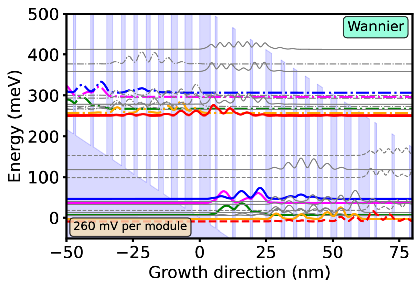
Figure 2: Wannier levels as in Fig. 1 under a constant electric field corresponding to a bias drop of 260 mV per module.

Here we assume a constant electric field $F$ providing $\phi(z)=Fz$ ($F$ is counted positive, if electrons with charge $-e$ are accelerated towards the right). The mean-field from the electron distribution and the ionized dopands provides a further contribution to $\phi(z)$, which is periodically repeated for the modules and can be directly included in the package. However, its implementation requires to solve a kinetic equation for electron populations separately. Most importantly, we assume a constant bias drop $Fd$ per module, which is the main parameter in the following. (This excludes the formation of field domains[21, 22, 23].)

III.1 Wannier-Stark States

We have an explicit expression for the matrix elements of the total Hamiltonian $\hat{H}^{F}=\hat{H}^{\textrm{het}}+\hat{H}^{\varphi}$ in the basis of Wannier levels, see Eqs. (18,19). This Hamiltonian can be diagonalized and the corresponding energy eigenstates are related to the Wanneir levels by a unitary transformation. These levels are orthonormal by construction.

The matrix elements of $\hat{H}^{F}$ in Wannier basis have the symmetry

$$H^{F}_{\nu n+h,\mu m+h}=H^{F}_{\nu n,\mu m}-eFd\delta_{n,m}\delta_{\nu,\mu}$$

This implies the labeling of the eigenlevels as $\psi^{\alpha n}(z)=\psi^{\alpha 0}(z-nd)$ and $E^{\textrm{WS}}_{\alpha n+h}=E^{\textrm{WS}}_{\alpha 0}-neFd$ for the infinite structure. These are known as Wannier-Stark (WS) levels [24]. In our code, we repeat the central module Nper times in each direction and choose the levels $\psi^{\alpha 0}(z)$ where the expectation value of $z$ is located within the central module. For other values of $n$, we apply the periodicity condition above for the functions and energies. We check explicitly the orthonormality between neighboring modules (default accuracy $10^{-4}$ in resource_QCL.calcZmat). Otherwise, Nper should be increased. Similar to the Wannier and Bloch levels, these functions $\psi(z)$ have a valence and conduction band component.

Fig. 3 shows the result. Comparing with the Wannier levels at the same bias drop per period in Fig. 2, the WS levels get typically repelled from each other resembling avoided crossings. The upper and lower extraction level are now approximately one and two optical phonon energies below the lower laser level, respectively, as targeted by the design.

Figure 3: Wannier-Stark (WS) levels obtained by diagonalising the matrix of the Hamiltonian in the basis of Wannier levels from Fig. 2. See Fig. 1 for labeling.

Now we want to point out, how this cumbersome approach to establish energy eigenstates via Bloch and Wannier functions is able to solve the problem of combined orthonormality and periodicity addressed in the introduction. The key problem in conventional calculations under applied bias is the need for a spatial boundary. Otherwise, the wave functions leak out to infinity. Here we work in the basis of Wannier functions, where we applied a cut-off in energy by restricting to a finite number of Bloch bands. This cut-off is relative to the conduction band edge and thus tilted under applied bias. Therefore, the states cannot leak out to infinity as this would require the coupling to states at high energy above the conduction band (which would be incorrect within the two-band model anyway).

III.2 EZ states

If WS levels are close in energy, they sometimes appear to be linear combinations of more localised states. Examples can be seen around 210 meV and -5 meV in Fig. 3. Such pairs of levels have to be treated with care, as they require a concise treatment of nondiagonal elements in the density matrix [25]. Thus it is helpful to disentangle theses states into a pair of localized states. This, however, provides a nondiagonal Hamiltonian containing tunneling matrix element between these levels.

Based on Ref. 26 this can be achieved by the following procedure: WS-levels that are close in energy are sorted into a multiplet. The maximal energy distance is set as gamma in resource_QCL.calcEZ with a default value of 5 meV. Within each multiplet the matrix of the Z-operator $\hat{z}$ is calculated and diagonalized. This provides a unitary transformation for the states within the multiplet. As the levels in the multiplet have approximately the same energy, the resulting diagonal elements of the Hamiltonian are rather similar, so that the energy $E$ of the levels are reasonably well defined, suggesting the denomination as EZ levels. The resulting levels of this procedure are shown in Fig. 4 for the device of Ref. 16. This demonstrates the spatial splitting of the extended states close to degeneracies.

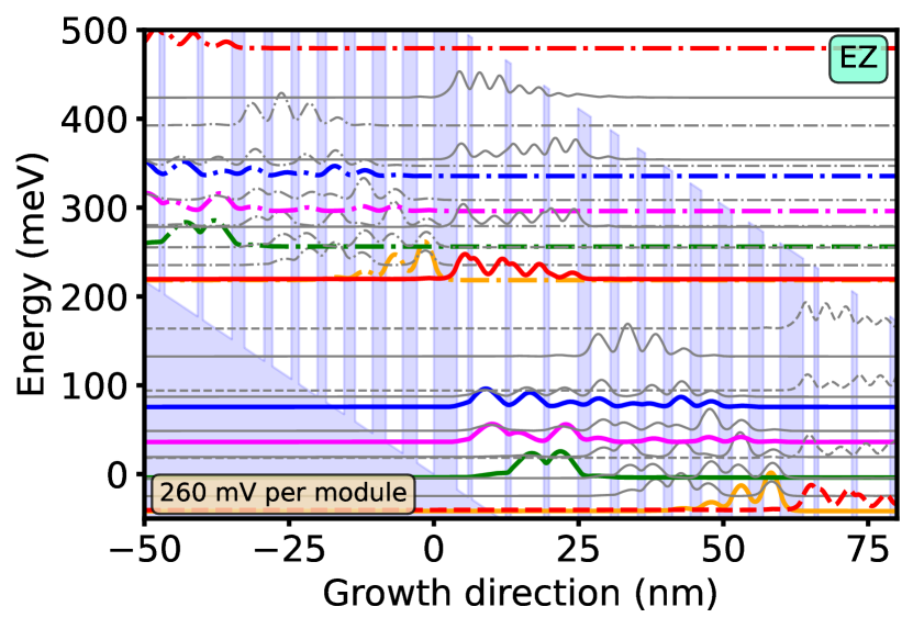
Figure 4: EZ levels obtained from the WS levels in Fig. 3 by unitary transformations within multiplets of levels, which are close in energy (here with gamma$=10$ meV). See Fig. 1 for labeling.

IV Conclusion

We presented a concise way to establish orthonormal sets of states for QCLs which satisfy the periodicity criterion. The presented Python package resource_QCL provides subroutines to establish Wannier, WS and, EZ states via unitary transformations from the initial Bloch states of the heterostructure without electrical potential. The respective two-component wave functions, the matrices for the Hamiltonian in the respective basis, and the $\hat{z}$-operator, as well as further quantities of interest are stored within a class for further usage. An example file example_to_use_resource_QCL.py is provided to demonstrate its usage.

The software has been tested for a large variety of QCL structures operating either in the infrared or THz range. The included plotting routine can be used to visualize the levels for a given structure. Equally important, the strictly orthonormal basis states establish a firm ground to calculate scattering matrix elements, optical transition strengths, etc, as required for quantum kinetic calculations.

References

- Faist et al. [1994] J. Faist, F. Capasso, D. L. Sivco, C. Sirtori, A. L. Hutchinson, and A. Y. Cho, “Quantum cascade laser,” Science 264, 553–556 (1994).
- Faist [2013] J. Faist, Quantum Cascade Lasers (Oxford University Press, Oxford, 2013).
- Botez and Belkin [2023] D. Botez and M. A. Belkin, eds., Mid-Infrared and Terahertz Quantum Cascade Lasers (Cambridge University Press, 2023).
- Jirauschek and Kubis [2014] C. Jirauschek and T. Kubis, “Modeling techniques for quantum cascade lasers,” Appl. Phys. Rev. 1, 011307 (2014).
- Wacker [2023] A. Wacker, “Simulating quantum cascade lasers: The challenge to quantum theory,” in Mid-Infrared and Terahertz Quantum Cascade Lasers, edited by D. Botez and M. A. Belkin (Cambridge University Press, 2023) p. 153–172.
- Kubis et al. [2009] T. Kubis, C. Yeh, P. Vogl, A. Benz, G. Fasching, and C. Deutsch, “Theory of nonequilibrium quantum transport and energy dissipation in terahertz quantum cascade lasers,” Phys. Rev. B 79, 195323 (2009).
- Burnett et al. [2018] B. A. Burnett, A. Pan, C. O. Chui, and B. S. Williams, “Robust density matrix simulation of terahertz quantum cascade lasers,” IEEE Trans. THz Sci. Techn. 8, 492–501 (2018).
- Baranov and Teissier [2015] A. N. Baranov and R. Teissier, “Quantum cascade lasers in the InAs/AlSb material system,” IEEE Journal of Selected Topics in Quantum Electronics 21, 85–96 (2015).
- Kato and Souma [2019] T. Kato and S. Souma, “Study of an application of non-parabolic complex band structures to the design for mid-infrared quantum cascade lasers,” Journal of Applied Physics 125, 073101 (2019).
- Kotera [2013] N. Kotera, “Energy dependence of electron effective mass and effect of wave function confinement in a nanoscale In0.53Ga0.47As/In0.52Al0.48As quantum well,” Journal of Applied Physics 113, 234314 (2013).
- Lee and Wacker [2002] S.-C. Lee and A. Wacker, “Nonequilibrium Green’s function theory for transport and gain properties of quantum cascade structures,” Phys. Rev. B 66, 245314 (2002).
- Lindskog, Winge, and Wacker [2013] M. Lindskog, D. O. Winge, and A. Wacker, “Injection schemes in THz quantum cascade lasers under operation,” Proc. SPIE 8846, 884603 (2013).
- White and Sham [1981] S. R. White and L. J. Sham, “Electronic properties of flat-band semiconductor heterostructures,” Phys. Rev. Lett. 47, 879 (1981).
- Bastard [1981] G. Bastard, “Superlattice band structure in the envelope-function approximation,” Phys. Rev. B 24, 5693–5697 (1981).
- Sirtori et al. [1994a] C. Sirtori, F. Capasso, J. Faist, and S. Scandolo, “Nonparabolicity and a sum rule associated with bound-to-bound and bound-to-continuum intersubband transitions in quantum wells,” Phys. Rev. B 50, 8663–8674 (1994a).
- Beck et al. [2002] M. Beck, D. Hofstetter, T. Aellen, J. Faist, U. Oesterle, M. Ilegems, E. Gini, and H. Melchior, “Continuous wave operation of a mid-infrared semiconductor laser at room temperature,” Science 295, 301 (2002).
- Note [1] The valence band component satisfies the same condition due to Eq. (3\@@italiccorr).
- Bruno-Alfonso and Nacbar [2007] A. Bruno-Alfonso and D. R. Nacbar, “Wannier functions of isolated bands in one-dimensional crystals,” Phys. Rev. B 75, 115428 (2007).
- Sirtori et al. [1994b] C. Sirtori, F. Capasso, D. L. Sivco, and A. Y. Cho, “Formation of new energy bands and minigap suppression by hybridization of barrier and well resonances in semiconductor superlattices,” Applied Physics Letters 64, 2982–2984 (1994b).
- Kohn [1959] W. Kohn, “Analytic properties of Bloch waves and Wannier functions,” Phys. Rev. 115, 809–821 (1959).
- Lu et al. [2006] S. L. Lu, L. Schrottke, S. W. Teitsworth, R. Hey, and H. T. Grahn, “Formation of electric-field domains in GaAs - AlxGa1-xAs quantum cascade laser structures,” Phys. Rev. B 73, 033311 (2006).
- Dhar et al. [2014] R. S. Dhar, S. G. Razavipour, E. Dupont, C. Xu, S. Laframboise, Z. Wasilewski, Q. Hu, and D. Ban, “Direct nanoscale imaging of evolving electric field domains in quantum structures,” Sci. Rep. 4, 7183 (2014).
- Almqvist et al. [2019] T. Almqvist, D. O. Winge, E. Dupont, and A. Wacker, “Domain formation and self-sustained oscillations in quantum cascade lasers,” Eur. Phys. J. B 92, 72 (2019).
- Wannier [1960] G. H. Wannier, “Wave functions and effective Hamiltonian for Bloch electrons in an electric field,” Phys. Rev. 117, 432–439 (1960).
- Callebaut and Hu [2005] H. Callebaut and Q. Hu, “Importance of coherence for electron transport in terahertz quantum cascade lasers,” J. Appl. Phys. 98, 104505 (2005).
- Rindert, Önder, and Wacker [2022] V. Rindert, E. Önder, and A. Wacker, “Analysis of high-performing terahertz quantum cascade lasers,” Phys. Rev. Applied 18, L041001 (2022).