Predictable and Performant Reactive Synthesis Modulo Theories via Functional Synthesis

Abstract

Reactive synthesis is the process of generating correct controllers from temporal logic specifications. Classical LTL reactive synthesis handles (propositional) LTL as a specification language. Boolean abstractions allow reducing $\textup{LTL}^{\mathcal{T}}$ specifications (i.e., LTL with propositions replaced by literals from a theory $\mathcal{T}$), into equi-realizable LTL specifications. In this paper we extend these results into a full static synthesis procedure. The synthesized system receives from the environment valuations of variables from a rich theory $\mathcal{T}$ and outputs valuations of system variables from $\mathcal{T}$. We use the abstraction method to synthesize a reactive Boolean controller from the LTL specification, and we combine it with functional synthesis to obtain a static controller for the original $\textup{LTL}^{\mathcal{T}}$ specification. We also show that our method allows adaptive responses in the sense that the controller can optimize its outputs in order to e.g., always provide the smallest safe values. This is the first full static synthesis method for $\textup{LTL}^{\mathcal{T}}$, which is a deterministic program (hence predictable and efficient).

1 Introduction

Reactive synthesis for Linear Temporal Logic (LTL) specifications [31] has received extensive research attention [33]. A specification $\varphi$ has its propositions split into those variables controlled by the system and the rest, controlled by the environment. A specification is realizable if there is a strategy for the system that produces valuations of the system variables such that all traces generated by the controller satisfy the specification. Realizability is the decision problem of whether such a strategy for the system exists. Synthesis is the process of generating one such winning strategy. Also, both problems are decidable for LTL [31].

A recent extension of LTL called $\textup{LTL}^{\mathcal{T}}$ (LTL modulo theories) allows replacing propositions with literals from a first-order theory $\mathcal{T}$. Given an $\textup{LTL}^{\mathcal{T}}$ specification $\varphi^{\mathcal{T}}$ an equi-realizable LTL $\varphi^{\mathbb{B}}$ formula can be generated, provided that the validity of $\mathcal{T}$ formulae of the form $\exists^{*}\forall^{*}$ is decidable [35, 37]. In $\textup{LTL}^{\mathcal{T}}$ synthesis the theory variables (for example Natural o Real) in the specification are split into environment-controlled and system-controlled variables, and both kinds can appear in any given literal, whereas in LTL an atomic proposition belongs exclusively to one player.

Note that a controller obtained from an off-the-shelf synthesis procedure for the Booleanized LTL formula $\varphi^{\mathbb{B}}$ cannot be directly used as a controller for $\varphi^{\mathcal{T}}$, because it must handle rich input and output values. Previous similar approaches either (1) focus on the satisfiability problem and not in realizability (e.g., [20, 22]); or (2) cannot be adapted to arbitrary $\mathcal{T}$ [27] or (3) do not guarantee termination [28, 39, 24], which makes these solutions incomplete. Recently, [36] presented a method for synthesis of a fragment of decidable $\textup{LTL}^{\mathcal{T}}$ specifications, which relies on the use of SMT solvers on-the-fly at every reaction, so it does not produce a standalone controller. This precludes the application to real embedded systems where controllers frequently operate because (1) the SMT solver is not guaranteed to terminate (particularly with limited resources), (2) the solver may not return the same values provided the same formula (affecting predictability) and (3) invoking solvers on the fly has an impact on the performance and the reaction time.

In this paper we present a static synthesis procedure for $\textup{LTL}^{\mathcal{T}}$ specifications. Our method proceeds as follows. We first obtain a Boolean controller $C$ for the equi-realizable Boolean specification $\varphi^{\mathbb{B}}$. The controller for $\varphi^{\mathcal{T}}$ uses two additional components: a $\<partitioner>$, that transforms the environment input $u$ into the corresponding Boolean input to $C$ and a $\<provider>$ that receives the input $u$ and the reaction from $C$, and produces the reaction $v$. Our $\<provider>$, instead of performing SMT calls, is implemented as a a collection of Skolem functions $f$ that generate, given $u$, an output $v$, such that the literals in $\varphi^{\mathcal{T}}$ agree with the reaction chosen by $C$. Since each trace produced by our controller satisfies $\varphi^{\mathcal{T}}$, the composition of the $\<partitioner>$, the Boolean controller $C$ and the $\<provider>$ is a controller for $\varphi^{\mathcal{T}}$ Therefore, the procedure described here is a static synthesis procedure for specifications in $\textup{LTL}^{\mathcal{T}}$. The resulting controller is standalone deterministic program, which is predictable and highly performant.

Next, we exploit the fact that we can synthesize Skolem functions that additionally receive a set of constraints to not only generate outputs that satisfy the desired literals, but that also optimize certain criteria from the set of possible correct outputs (e.g., to provide the smallest value among possible values). We call this technique adaptivity. All these results are applicable to $\textup{LTL}^{\mathcal{T}}$ on infinite or on finite traces, using appropriate synthesis tools for the resulting $\varphi^{\mathbb{B}}$.

In summary, the contributions of this paper are: (1) a formalization and soundness proof of the controller architecture for synthesis for $\textup{LTL}^{\mathcal{T}}$; (2) a derived correct method to synthetise static controllers from $\textup{LTL}^{\mathcal{T}}$ specifications combining Boolean abstraction, reactive synthesis and functional synthesis; (3) a formalization of the limits and capabilities of using Skolem functions, showing their power to model adaptivity; (4) an extensive empirical evaluation that shows our method predictable and fast. To the best of our knowledge, this is the first full static reactive synthesis approach for $\textup{LTL}^{\mathcal{T}}$ specifications. Moreover, since our approach leverages off-the-shelf components (reactive synthesis, functional synthesis), it would immediately benefit from advances in those areas and also from discoveries in decidable fragments of $\textup{LTL}^{\mathcal{T}}$ realizability. The remainder of the paper is structured as follows. Sec. 2 contains preliminary definitions, including the Boolean abstraction method from [35] and a running example that is used in the rest of the paper. Sec. 3 formalizes the controller architecture and proves its correctness. Sec. 4 introduces an adaptive extension of our approach. Sec. 5 contains an empirical evaluation. Sec. 6 shows related work and concludes.

2 Preliminaries

2.0.1 First-order Theories.

In this paper we use first-order theories. We describe theories with single domain for simplicity, but this can be easily extended to multiple sorts. A first-order theory $\mathcal{T}$ (see e.g., [7]) is described by a signature $\Sigma$, which consists of a finite set of functions and constants, a set of variables and a domain. The domain $\mathbb{D}$ of a theory $\mathcal{T}$ is the sort of its variables. For example, the domain of non-linear real arithmetic $\mathcal{T}_{\mathbb{R}}$ is $\mathbb{R}$ and we denote this by $\mathbb{D}(\mathcal{T}_{\mathbb{R}})=\mathbb{R}$ or simply by $\mathbb{D}$ if it is clear from the context. A formula $\varphi$ is valid in $\mathcal{T}$ if, for every interpretation $I$ of $\mathcal{T}$, then $I\vDash\varphi$. A fragment of a theory $\mathcal{T}$ is a syntactically-restricted subset of formulae of $\mathcal{T}$. Given a formula $\psi$, we use $\psi[\overline{x}\leftarrow\overline{u}]$ for the substitution of variables $\overline{x}$ by terms $\overline{u}$ (typically constants).

2.0.2 Reactive Synthesis.

We fix a finite set of atomic propositions $\mathit{AP}$. Then, $\Sigma=2^{\mathit{AP}}$ is the alphabet of valuations, and $\Sigma^{*}$ and $\Sigma^{\omega}$ are the set of finite and infinite traces respectively. Given a trace $\sigma$ we use $\sigma(i)$ for the letter at position $i$ and $\sigma^{i}$ for the suffix trace that starts at position $i$. The syntax of propositional LTL [31, 29] is:

$$\varphi::=\top\;\hskip 1.99997pt\big{|}\hskip 1.99997pt\;a\;\hskip 1.99997pt\big{|}\hskip 1.99997pt\;\varphi\lor\varphi\;\hskip 1.99997pt\big{|}\hskip 1.99997pt\;\neg\varphi\;\hskip 1.99997pt\big{|}\hskip 1.99997pt\;\LTLcircle\varphi\;\hskip 1.99997pt\big{|}\hskip 1.99997pt\;\varphi\mathbin{\mathcal{U}}\varphi$$

where $a\in\mathit{AP}$; $\lor$, $\land$ and $\neg$ are the usual Boolean disjunction, conjunction and negation; and and $\mathbin{\mathcal{U}}$ are the next and until temporal operators. The semantics of LTL associates traces $\sigma\in\Sigma^{\omega}$ with LTL fomulae as follows:

$$\begin{array}[]{l@{\hspace{0.3em}}c@{\hspace{0.3em}}l}\sigma\models\top\hfil\hskip 3.00003pt&\hfil\hskip 3.00003pt&\text{always holds}\\ \sigma\models a\hfil\hskip 3.00003pt&\text{iff }\hfil\hskip 3.00003pt&a\in\sigma(0)\\ \sigma\models\varphi_{1}\mathrel{\vee}\varphi_{2}\hfil\hskip 3.00003pt&\text{iff }\hfil\hskip 3.00003pt&\sigma\models\varphi_{1}\text{ or }\sigma\models\varphi_{2}\\ \sigma\models\neg\varphi\hfil\hskip 3.00003pt&\text{iff }\hfil\hskip 3.00003pt&\sigma\not\models\varphi\\ \sigma\models\LTLcircle\varphi\hfil\hskip 3.00003pt&\text{iff }\hfil\hskip 3.00003pt&\sigma^{1}\models\varphi\\ \sigma\models\varphi_{1}\mathbin{\mathcal{U}}\varphi_{2}\hfil\hskip 3.00003pt&\text{iff }\hfil\hskip 3.00003pt&\text{for some }i\geq 0\;\;\sigma^{i}\models\varphi_{2},\text{ and }\text{for all }0\leq j<i,\sigma^{j}\models\varphi_{1}\\ \end{array}$$

We use common derived operators like $\vee$, $\mathcal{R}$, and . Reactive synthesis [33, 32, 5, 17] is the problem of automatically constructing a system based on an LTL specification $\varphi$, where the atomic propositions of $\varphi$ ($\mathit{AP}$) are divided into propositions $\overline{e}=\mathit{Vars}_{E}(\varphi)$ controlled by the environment and $\overline{s}=\mathit{Vars}_{S}(\varphi)$ controlled by the system (with $\overline{e}\cup\overline{s}=\mathit{AP}$ and $\overline{e}\cap\overline{s}=\emptyset$). A reactive specification corresponds to a turn-based game where the environment and system players alternate. In each turn, the environment produces values for $\overline{e}$, and the system responds with values for $\overline{s}$. A valuation is a map from $\overline{e}$ into $\mathbb{B}$ (similarly for $\overline{s}$). We use $\mathit{val}(\overline{e})$ and $\mathit{val}(\overline{s})$ for valuations. A play is an infinite sequence of turns and induces a trace $\sigma$ by joining at each position the valuations that the environment and system players choose. The system player wins a play if the trace satisfies $\varphi$. A strategy for the system is a tuple $\rho:\langle Q,q_{0},\delta,o\rangle$ where $Q$ is a finite set of states, $q_{0}\in Q$ is the inital state, $\delta:Q\times\mathit{val}(\overline{e})\mathrel{\rightarrow}Q$ is the transition function and $o:Q\times\mathit{val}(\overline{e})\mathrel{\rightarrow}\mathit{val}(\overline{s})$ is the output function. A play $((\overline{e}_{0},\overline{s}_{0}),(\overline{e}_{1},\overline{s}_{1}),\ldots)$ is played according to $\rho$ if the sequence $((\overline{e}_{0},\overline{s}_{0},q_{0}),(\overline{e}_{1},\overline{s}_{1},q_{1}),\ldots)$ satisfies that $q_{i+1}=\delta(q_{i},\overline{e}_{i})$ and $\overline{s}_{i}=o(q_{i},\overline{e}_{i})$ for all $i\geq 0$. A strategy $\rho$ is wining for the system if all plays played according to $\rho$ satisfy $\varphi$. We will use strategy and controller interchangeably.

2.0.3 Linear Temporal Logic Modulo Theories.

The syntax of $\textup{LTL}^{\mathcal{T}}$ replaces atoms $a$ by literals $l$ from theory $\mathcal{T}$. We use $\mathit{Vars}(l)$ for the variables in literal $l$ and $\mathit{Vars}(\varphi)$ for the union of the variables that occur in the literals of $\varphi$. A valuation for a set of vars $\overline{z}$ is a map from $\overline{z}$ into $\mathbb{D}$. The alphabet of a formula $\varphi$ is $\Sigma_{\mathcal{T}}:\mathit{Vars}(\varphi)\mathrel{\rightarrow}\mathbb{D}$. The semantics of $\textup{LTL}^{\mathcal{T}}$ associate traces $\sigma\in\Sigma_{\mathcal{T}}^{\omega}$ with formulae, where for atomic propositions $\sigma\models l$ holds iff $\sigma(0)\vDash_{\mathcal{T}}l$, that is, if the valuation $\sigma(0)$ makes the literal $l$ true. The rest of the operators are as in LTL.

For realizability and synthesis from $\textup{LTL}^{\mathcal{T}}$, the variables in $\mathit{Vars}(\varphi)$ are split into those variables controlled by the environment ($\overline{x}$ or $\mathit{Vars}_{E}(\varphi)$) and those controlled by the system ($\overline{y}$ or $\mathit{Vars}_{E}(\varphi)$). We use $\varphi(\overline{x},\overline{y})$ to denote that $\overline{x}\cup\overline{y}$ are the variables occurring in $\varphi$ (where $\overline{x}\cup\overline{y}=\mathit{Vars}(\varphi)$ and $\overline{x}\cap\overline{y}=\emptyset$). A trace is an infinite sequence of valuations of $\overline{x}$ and $\overline{y}$, which induces an infinite sequence of Boolean values for each of the literals at each position, and ultimately a valuation of $\varphi$. For instance, given $\psi=\LTLsquare(y>x)$ the trace $(\langle x:4,y:5\rangle,\langle x:9,y:7\rangle,\ldots)$ induces $(\langle l:\textit{true}\rangle,\langle l:\textit{false}\rangle,\ldots)$ for the literal $l=(y>x)$. An $\textup{LTL}^{\mathcal{T}}$ specification corresponds to a game with an infinite arena, where positions can have infinitely many successors. A strategy now for the system is a tuple $\rho^{\mathcal{T}}:\langle Q,q_{0},\delta,o\rangle$ where $Q$ and $q_{0}$ are as before and $\delta:Q\times\mathit{val}(\overline{x})\mathrel{\rightarrow}Q$ is the transition function and $o:Q\times\mathit{val}(\overline{x})\mathrel{\rightarrow}\mathit{val}(\overline{y})$ is the output function.

2.0.4 Boolean Abstraction.

The Boolean abstraction method [35] transforms an $\textup{LTL}^{\mathcal{T}}$ specification $\varphi^{\mathcal{T}}$ into an equi-realizable LTL specification $\varphi^{\mathbb{B}}$. The resulting LTL formula can be passed to an off-the-shelf synthesis engine, which generates a controller for realizable specifications. The process of Boolean abstraction involves transforming an input formula $\varphi^{\mathcal{T}}$, which contains literals $l_{i}$, into a new specification $\varphi^{\mathbb{B}}=\varphi^{\mathcal{T}}[l_{i}\leftarrow s_{i}]\wedge\varphi^{\textit{extra}}$, where $\overline{s}=\{s_{i}|\text{for each }l_{i}\}$ is a set of fresh atomic propositions controlled by the system—such that $s_{i}$ replaces $l_{i}$—and where $\varphi^{\textit{extra}}$ is an additional sub-formula that captures the dependencies between the $\overline{s}$ variables. The formula $\varphi^{\textit{extra}}$ also includes additional environment variables $\overline{e}$ (controlled by the environment) that encode the power of the environment to leave the system with the power to choose certain valuations of the variables $\overline{s}$. The formula $\varphi^{\textit{extra}}$ also constraints the environment in such a way that exactly one of the variables in $\overline{e}$ is true.

A choice $c$ is a valuation of $\overline{s}$, $c(s_{i})=\textit{true}$ means that $s_{i}$ is in the choice. We write $s_{i}\in c$ as a synonym of $c(s_{i})=\textit{true}$. The characteristic formula $f_{c}(\overline{x},\overline{y})$ of a choice $c$ is $f_{c}=\bigwedge_{s_{i}\in c}l_{i}\mathrel{\wedge}\bigwedge_{s_{i}\notin c}\neg l_{i}.$ Note that we often represent choices as valuation $v_{\overline{s}}$ of the Boolean variables $\overline{s}$ (which map each variable in $\overline{s}$ to true or false). We use $\mathcal{C}$ for the set of choices (that is, the set of sets of $\overline{s}$). A reaction $r\subset\mathcal{C}$ is a set of choices, which characterizes the possible responses of the system as the result of a move by the environment. The characteristic formula $f_{r}(\overline{x})$ of a reaction $r$ is:

$$(\bigwedge_{c\in r}\exists\overline{y}.f_{c})\mathrel{\wedge}(\bigwedge_{c\notin r}\forall\overline{y}\neg f_{c})$$

A reaction $r$ is valid whenever $\exists\overline{x}.f_{r}(\overline{x})$ is valid.

Intuitively, $f_{r}$ states that for some valuations of the variables $\overline{x}$ controlled by the environment, the system can respond with valuations of $\overline{y}$ making the literals in some choice $c\in r$ but cannot respond with valuations making the literals in choices $c\notin r$. The set of valid reactions partitions precisely the moves of the environment in terms of the reaction power left to the system. For each valid reaction $r$ there is a fresh environment variable $e\in\overline{e}$. Hence, the restriction in $\varphi^{\textit{extra}}$ that forces the environment to make exactly one variable in $\overline{e}$ true corresponds to the environment choosing a reaction $r$ (when the corresponding $e$ is true).

Boolean abstraction [35] uses the set of valid reactions to produce an equi-realizable $\varphi^{\mathbb{B}}$ from a formula $\varphi^{\mathcal{T}}$, which are in the same temporal fragment.

Example 1 (Running example)

Let $\varphi^{\mathcal{T}}(\overline{x},\overline{y})$ be the following specification (where $\overline{x}=\{x\}$ is controlled by the environment and $\overline{y}=\{y\}$ by the system):

$$\varphi^{\mathcal{T}}=\square\big{[}\big{(}(x<2)\mathrel{\rightarrow}\LTLcircle(y>1)\big{)}\mathrel{\wedge}\big{(}(x\geq 2)\shortrightarrow(y\leq x)\big{)}\big{]}.$$

In theory $\mathcal{T}_{\mathbb{Z}}$ this specification is realizable (consider the strategy to always play $y=2$). In this theory, the Boolean abstraction first introduces $s_{0}$ to abstract $(x<2)$, $s_{1}$ to abstract $(y>1)$ and $s_{2}$ to abstract $(y\leq x)$. Then $\varphi^{\mathbb{B}}=\varphi^{\prime\prime}\wedge\LTLsquare(\varphi^{\textit{legal}}\mathrel{\rightarrow}\varphi^{\textit{extra}})$ where $\varphi^{\prime\prime}=(s_{0}\shortrightarrow\LTLcircle s_{1})\wedge(\neg s_{0}\shortrightarrow s_{2})$ is a direct abstraction of $\varphi^{\mathcal{T}}$. Finally, $\varphi^{\textit{extra}}$ captures the depenencies between the abstracted variables:

$$\varphi^{\textit{extra}}: \begin{pmatrix}\begin{array}[]{lrcl}\phantom{\wedge}&\big{(}e_{0}&\mathrel{\rightarrow}&\big{(}[\phantom{\neg}s_{0}\wedge s_{1}\wedge\neg s_{2}]\vee[\phantom{\neg}s_{0}\wedge\neg s_{1}\wedge s_{2}]\big{)}\\[2.70004pt] \wedge&\big{(}e_{1}&\mathrel{\rightarrow}&\big{(}[\neg s_{0}\wedge s_{1}\wedge\neg s_{2}]\vee[\neg s_{0}\wedge\neg s_{1}\wedge\phantom{\neg}s_{2}]\vee[\neg s_{0}\wedge\phantom{\neg}s_{1}\wedge\neg s_{2}]\big{)}\end{array}\end{pmatrix}$$

and $\varphi^{\textit{legal}}:(e_{0}\vee e_{1})\wedge(e_{0}\leftrightarrow\neg e_{1})$, where $\overline{e}=\{e_{0},e_{1}\}$ belong to the environment and represent $(x<2)$ and $(x\geq 2)$, respectively. Thus, $\varphi^{\textit{legal}}$ encodes that $e_{0}$ and $e_{1}$ characterize a partition of the (infinite) input valuations of the environment (and that precisely one of $\overline{e}$ are true in every move). For example, the valuation $v_{e}=\langle e_{0}:\textit{false},e_{1}:\textit{true}\rangle$ of $\overline{e}$ corresponds to the choice of the environment where only $e_{1}$ is true. Sub-formulae like $(s_{0}\wedge s_{1}\wedge\neg s_{2})$ represent the choices of the system (in this case, $c=\{s_{0},s_{1}\}$), that is, given a decision of the environment (a valuation of $\overline{e}$ that makes exactly one variable $e$ true), the system can react with one of the choices $c$ in the disjunction implied by $e$. We denote $c_{0}=\{s_{0},s_{1},s_{2}\}$, $c_{1}=\{s_{0},s_{1}\}$, $c_{2}=\{s_{0},s_{2}\}$, $c_{3}=\{s_{0}\}$, $c_{4}=\{s_{1},s_{2}\}$, $c_{5}=\{s_{1}\}$, $c_{6}=\{s_{2}\}$ and $c_{7}=\emptyset$. Note that e.g., $c_{1}$ can be represented as $v_{\overline{s}}=\langle s_{0}:\textit{true},s_{1}:\textit{true},s_{2}:\textit{false}\rangle$.

3 Static Reactive Synthesis Modulo Theories

The Boolean abstraction method [35] reduces an $\textup{LTL}^{\mathcal{T}}$ formula $\varphi^{\mathcal{T}}$ into an equi-realizable LTL specification $\varphi^{\mathbb{B}}$, but it does not present a synthesis procedure for $\varphi^{\mathcal{T}}$. We solve this problem here by providing a full static synthesis method for $\textup{LTL}^{\mathcal{T}}$. Our procedure builds a controller for realizable $\varphi^{\mathcal{T}}$ specifications that handles inputs and outputs from a rich domain $\mathbb{D}(\mathcal{T})$, using as a building block the synthetized Boolean controller for $\varphi^{\mathbb{B}}$ and other two sub-components.

3.1 Formal Architecture

Figure 1: A controller architecture for reactive synthesis of $\textup{LTL}^{\mathcal{T}}$ specifications.

We call our approach static $\textup{LTL}^{\mathcal{T}}$ synthesis (see Fig. 1). Our method starts from $\varphi^{\mathcal{T}}(\overline{x},\overline{y})$ and statically generates a Boolean controller $\rho^{\mathbb{B}}$ for $\varphi^{\mathbb{B}}$ and combines it with a $\<partitioner>$ and a $\<provider>$ (generated from the abstraction process of $\varphi^{\mathcal{T}}$ to $\varphi^{\mathbb{B}}$) handle the inputs and outputs from $\mathbb{D}$. At run-time, at each instant the resulting controller follows these steps:

1. a valuation $v_{\overline{x}}\in\mathit{val}(\overline{x})$ is provided by the environment;

2. the $\<partitioner>$ discretizes $v_{\overline{x}}$ generating a Boolean valuation $v_{\overline{e}}\in\mathit{val}(\overline{e})$ of input variables for $\rho^{\mathbb{B}}$.

3. $\rho^{\mathbb{B}}$ responds with a valuation $v_{\overline{s}}\in\mathit{val}(\overline{s})$ of the variables $\overline{s}$ that $\rho^{\mathbb{B}}$ controls.

4. the $\<provider>$ produces a valuation $v_{\overline{y}}\in\mathit{val}(\overline{y})$ of the output variables that together with $v_{\overline{x}}$ guarantee that the literals from $\varphi^{\mathcal{T}}$ will be evaluated as indicated by the choice $c$ that corresponds to $v_{\overline{s}}$ indicated by $\rho^{\mathbb{B}}$. This step corresponds to finding a model of $\exists\overline{y}.f_{c}([\overline{x}\leftarrow v_{\overline{x}}],\overline{y})$.

For step (4) one approach is to invoke an SMT solver on the fly to generate models (proper values of $v_{\overline{y}}$), which is guaranteed to be satisfiable (by the soundness of the Boolean abstraction method). However, most uses of controllers cannot use SMT solvers dynamically. Moreover, note that the formula to be solved has quantifier alternations (within $f_{c}$) which is currently challenging for state-of-the art SMT solving technology for many theories. In this paper we present an alternative: a method that produces a totally static controller, using Skolem functions associated to each $(e,c)$ pair. These Skolem functions are models of the formula

$$\forall\overline{x}.\exists\overline{y}.f_{r}(\overline{x})\mathrel{\rightarrow}f_{c}(\overline{x},\overline{y})$$

Recall that $f_{r}(\overline{x})$ is the formula that characterizes the environment valuations for which $r$ captures the possible responses after receiving $\overline{x}$, according to reasoning in the theory $\mathcal{T}$.

3.1.1 Partitioner.

At each timestep, the partitioner receives a valuation $v_{\overline{x}}\in\mathit{val}(\overline{x})$ of the environment variables and finds the input variable $e_{k}$ to be fed to the Boolean controller. The partitioner must find the entry $(e,r)$ in the table of valid reactions for which $f_{r}(v_{\overline{x}})$ is valid and return $e$. For instance, recall partitions $e_{0}$ and $e_{1}$ from Ex. 1, then an input trace $(\langle x:4\rangle,\langle x:4\rangle,\langle x:1\rangle,\langle x:0\rangle,\langle x:2\rangle,\ldots)$ will be partitioned into $(\langle e:e_{1}\rangle,\langle e:e_{1}\rangle,\langle e:e_{0}\rangle,\langle e:e_{0}\rangle,\langle e:e_{1}\rangle,\ldots)$ (for simplicity, here we show the only Boolean variable $e_{i}$ that is true). The following defines a legal partitioner.

Definition 1

Let $\varphi^{\mathcal{T}}(\overline{x},\overline{y})$ be an $\textup{LTL}^{\mathcal{T}}$ specification and $\varphi^{\mathbb{B}}(\overline{e},\overline{s})$ its Boolean abstraction. A $\<partitioner>$ is a function $\alpha:\mathit{val}(\overline{x})\mathrel{\rightarrow}\overline{e}$ such that if $(e,r)$ is a valid reaction and $f_{r}[\overline{x}\leftarrow v_{\overline{x}}]$ is valid, then $\alpha(v_{\overline{x}})=e$.

Note that, by the soundness of the Boolean abstraction method, there is one

Input: $v_{\overline{x}}\in\mathit{val}(\overline{x})$

forall $(e,r)\in\textit{VR}(\varphi)$ do

       if $f_{r}[\overline{x}\leftarrow v_{\overline{x}}]$ is valid then

             return $e$

            

      

Alg. 1 A brute force partitioner $\alpha$.

and only one such candidate $e$ for every input $v_{\overline{x}}$. Note that $\alpha(v_{\overline{x}})=e$ induces a valuation $v_{\overline{e}}$ of the variables $\overline{e}$ by $v_{\overline{x}}(e)=\textit{true}$ and $v_{\overline{x}}(e^{\prime})=\textit{false}$ for all other $e^{\prime}\neq e$. Alg. 1 shows a brute force method to find variable $e$.

3.1.2 Controller.

The Boolean $\<controller>$ receives the discrete environment input $v_{\overline{e}}$ and produces a discrete output $v_{\overline{s}}$ that represents the selected choices according to a winning strategy for $\varphi^{\mathbb{B}}$. This controller $\rho^{\mathbb{B}}$ can obtained using off-the-shelf reactive synthesis tools. This controller $\rho^{\mathbb{B}}$ produces a valuation $v_{\overline{s}}\in\mathit{val}(\overline{s})$ at every step, guaranteeing that the trace produced satisfies $\varphi^{\mathbb{B}}$.

Consider an instant where only $e$ is true in the input $v_{\overline{e}}$, and let $r$ be the valid reaction corresponding to $e$; then if $v_{\overline{s}}$ is the output produced by $\rho^{\mathbb{B}}$ from $v_{\overline{e}}$ the choice $c:\{s_{i}|v_{\overline{s}}(s_{i})=\textit{true}\}$ belongs to $c\in r$. This is forced by the $\varphi^{\textit{extra}}$ constraint in the construction of $\varphi^{\mathbb{B}}$ from $\varphi^{\mathcal{T}}$ in the Boolean abstraction method. To better illustrate this, recall Ex. 1 and among the possible winning strategies that the system has, consider the following. If $v_{\overline{e}}$ is $\langle e_{0}:\textit{true},e_{1}:\textit{false}\rangle$, then the output choice $v_{\overline{s}}$ is $\langle s_{0}:\textit{true},s_{1}:\textit{true},s_{2}:\textit{false}\rangle$ (i.e., $c_{1}$). On the other hand, if $v_{\overline{e}}(e_{1})$ is $\langle e_{0}:\textit{false},e_{1}:\textit{true}\rangle$ then output choice $v_{\overline{s}}$ is $\langle s_{0}:\textit{false},s_{1}:\textit{true},s_{2}:\textit{true}\rangle$ (i.e., $c_{4}$).

3.1.3 Provider.

The discrete behavior of the Boolean controller requires an additional component that produces a valuation $v_{\overline{y}}\in\mathit{val}(\overline{y})$ of the system variables over $\overline{y}$ satisfying $\varphi^{\mathcal{T}}$. The $\<provider>$ receives the choice and the input $v_{\overline{x}}\in\mathit{val}(\overline{x})$, and substitutes $v_{\overline{x}}$ for $\overline{x}$ in $f_{c}$: $f_{c}([\overline{x}\leftarrow v_{\overline{x}}],\overline{y})$. The goal of the provider is to find a proper valuation for $\overline{y}$.

Definition 2 (Provider)

A $\<provider>$ is a function $\beta:\mathit{val}(\overline{x})\times\mathit{val}(\overline{s})\mathrel{\rightarrow}\mathit{val}(\overline{y})$ such that for every $v_{\overline{x}}\in\mathit{val}(\overline{x})$ and choice $c\in\mathit{val}(\overline{s})$ , the following holds

$$f_{c}(\overline{x}\leftarrow v_{\overline{x}},\overline{y}\leftarrow\beta(v_{\overline{x}},c)).$$

We will show below that if $v_{\overline{x}}$ is an input to a $\<partitioner>$, $r$ is the valid corresponding reaction, and $c$ is one of the winning choices of the controller (that is, $c\in r$), then the following formula is valid.

$$[\exists\overline{y}.f_{c}(\overline{y},\overline{x}\leftarrow v_{\overline{x}})]$$

This formula can be discharged into a solver with capabilities to produce a model $v_{\overline{y}}$ (e.g., an SMT solver like Z3 [13]), which is exactly the dynamic approach presented at [36].

Example 2

Consider again Ex. 1 and input trace $(\langle x:4\rangle,\langle x:4\rangle,\langle x:1\rangle,\langle x:0\rangle,\langle x:2\rangle,\ldots)$. This trace is mapped into the following discrete input trace $(\langle c:c_{4}\rangle,\langle c:c_{4}\rangle,\langle c:c_{1}\rangle,\langle c:c_{1}\rangle,\langle c:c_{4}\rangle,\ldots)$. Recall that $s_{0}$ abstracts $(x<2)$, $s_{1}$ abstracts $(y>1)$ and $s_{2}$ abstracts $(y\leq x)$. Then, the output trace must be a sequence $v_{\overline{y}}$ of values of $y$ such that the following holds:

$$\begin{array}[]{r@{}ll}(&[\neg(4<2)\wedge(y>1)\wedge\phantom{\neg}(y\leq 4)],\\ &[\neg(4<2)\wedge(y>1)\wedge\phantom{\neg}(y\leq 4)],\\ &[\phantom{\neg}(1<2)\wedge(y>1)\wedge\neg(y\leq 1)],\\ &[\phantom{\neg}(0<2)\wedge(y>1)\wedge\neg(y\leq 0)],\\ &[\neg(2<2)\wedge(y>1)\wedge\phantom{\neg}(y\leq 2)],\ldots)\end{array}$$

One such possible sequence is $(\langle y:2\rangle,\langle y:2\rangle,\langle y:2\rangle,\langle y:2\rangle,\langle y:2\rangle,\ldots)$. Note how $\overline{x}$ is replaced in each timestep by concrete input $v_{\overline{x}}$. However, many different values $v_{\overline{y}}$ exist that satisfy the output trace (e.g. $(\langle y:2\rangle,\langle y:3\rangle,\langle y:3\rangle,\langle y:4\rangle,\langle y:2\rangle,\ldots)$.)

3.1.4 Correctness.

The Boolean system strategy $\rho^{\mathbb{B}}:\langle Q,q_{0},\delta,o\rangle$ for $\varphi^{\mathbb{B}}$ produces, at every timestep, a valuation of $\overline{s}$ from a valuation of $\overline{e}$. We now define a strategy $\rho^{\mathcal{T}}$ of the system in $\varphi^{\mathcal{T}}$ and prove that all moves played according to $\rho^{\mathcal{T}}$ are winning for the system; i.e., all produced traces satisfy $\varphi^{\mathcal{T}}$. Intuitively, $\rho^{\mathcal{T}}$ composes the $\<partitioner>$, which translates inputs to the Boolean controller, collects the move chosen by the Boolean controller and then uses the $\<provider>$ to generate an output.

Definition 3 (Combined Strategy)

Given a $\<partitioner>$ $\alpha$, a controller $\rho^{\mathbb{B}}$ for $\varphi^{\mathbb{B}}$ and a $\<provider>$ $\beta$, the strategy $\rho^{\mathcal{T}}:\langle Q^{\prime},q_{0}^{\prime},\delta^{\prime},o^{\prime}\rangle$ for $\varphi^{\mathcal{T}}$ is:

• $Q^{\prime}=Q$ and $q_{0}^{\prime}=q_{0}$,

• $\delta^{\prime}(q,v_{\overline{x}})=\delta(q,v_{\overline{e}})$ where $v_{\overline{e}}=\alpha(v_{\overline{x}})$,

• $o^{\prime}(q,v_{\overline{x}})=\beta(v_{\overline{x}},c)$ where $c=o(q,v_{\overline{x}})$.

We use $C(\alpha,\rho^{\mathbb{B}},\beta)$ for the combined strategy of $\alpha$, $\rho^{\mathbb{B}}$ and $\beta$. Now we are ready to state the main theorem.

Theorem 3.1 (Correctness of Synthesis Modulo Theories)

Let $\varphi^{\mathcal{T}}$ be a realizable specification, $\varphi^{\mathbb{B}}$ its Boolean abstraction, $\alpha$ a $\<partitioner>$ and $\beta$ a $\<provider>$. Let $\rho^{\mathbb{B}}$ be a winning strategy for $\varphi^{\mathbb{B}}$, and let $\rho^{\mathcal{T}}=C(\alpha,\rho^{\mathbb{B}},\beta)$ be the combined strategy. Then $\rho^{\mathcal{T}}$ is winning for $\varphi^{\mathcal{T}}$.

Proof

(Sketch). Let $\rho^{\mathbb{B}}:\langle Q,q_{0},\delta,o\rangle$ and $\rho^{\mathcal{T}}:\langle Q,q_{0},\delta^{\prime},o^{\prime}\rangle$ be the strategies. Let $\pi=((\overline{x}_{0},\overline{y}_{0},q_{0}),(\overline{x}_{1},\overline{y}_{1},q_{1}),\ldots)$ be an infinite sequence played according to $\rho^{\mathcal{T}}$, that is $\overline{y}_{i}=o^{\prime}(q_{i},\overline{x}_{i})$ and $q_{i+1}=\delta^{\prime}(q_{i},\overline{x}_{i})$. Consider the sequence $((\overline{e}_{0},\overline{s}_{0},q_{0})$, $(\overline{e}_{1},\overline{s}_{1},q_{1}),\ldots)$ such that $\overline{e}_{i}=\alpha(\overline{x}_{i})$, $\overline{s}_{i}=o(q_{i},\overline{e}_{i})$ and $q_{i+1}=\delta(q_{i},\overline{e}_{i})$. Note that this a play of $\varphi^{\mathbb{B}}$ played according to $\rho^{\mathbb{B}}$ so it satisfies $\varphi^{\mathbb{B}}$. In particular, it satisfies $\varphi^{\textit{extra}}$. Moreover, for every time instant $i$, $\overline{y}_{i}=\beta(\overline{x}_{i},\overline{s}_{i})$ by construction. It follows that, for every $i$, every literal $l_{i}$ in $\varphi^{\mathcal{T}}$ and the corresponding $s_{i}$ in $\varphi^{\mathbb{B}}$ have the same valuation. By structural induction, all corresponding sub-formulae of $\varphi^{\mathbb{B}}$ and $\varphi^{\mathcal{T}}$ have the same valuation at every position. Therefore, $\pi\models\varphi^{\mathcal{T}}$. ∎

3.2 Standalone Synthesis Modulo Theories

3.2.1 Static Provider.

As stated above, a $\<provider>$ produces, at every step, a model of a (satisfiable) formula (where some of the elements in the formula are the inputs received at that specific step). This can be implemented using an SMT solver at every step. In this paper we propose an alternative approach where we produce at static time a $\<provider>$ via the functional synthesis of a Skolem function. The controller then invokes the function produced instead of using dynamic queries to an SMT solver. Given an arbitrary relation $R(x,y)$ a Skolem function is a function $\mathtt{h}$ that witnesses the validity of $\forall x.\exists y.R(x,y)$ by guaranteeing that $\forall x..R(x,\mathtt{h}(x))$ is valid. Recall that a correct $\<provider>$ is a function $\beta:\mathit{val}(\overline{x})\times\mathit{val}(\overline{s})\mathrel{\rightarrow}\mathit{val}(\overline{y})$ which is a witness of the validity of the following formula:

$$\forall\overline{x}.\exists\overline{y}.f_{r}(\overline{x})\mathrel{\rightarrow}f_{c}(\overline{x},\overline{y})$$

for a given reaction $r$ and choice $c\in r$. A Skolem function for $c$ is a function $\mathtt{h}_{c}:\mathit{val}(\overline{x})\mathrel{\rightarrow}\mathit{val}(\overline{y})$ such that the following is valid:

$$\forall\overline{x}.f_{r}(\overline{x})\mathrel{\rightarrow}f_{c}(\overline{x},h_{c}(\overline{x}))$$

For instance, consider a specification where the environment controls an integer variable $x$ and the system controls an integer variable $y$ in the specification $\varphi^{\mathcal{T}}=\LTLsquare(y>x)$. A Skolem function $\mathtt{h}(x)=x+1$ serves as a witness (providing values for $y$) of the validity of $\forall x.\exists y.(\top\mathrel{\rightarrow}(y>x))$ and can be used to provide correct integer values for $y$. For many theories, Skolem functions for $\beta$ can be statically computed, which means that we can generate statically a $\<provider>$ for these theories, and in turn, a full static controller for $\varphi^{\mathcal{T}}$. In this paper, we used the AEval funtional synthesis tool  [16], which generates witnessing Skolem functions for (possibly many) existentially-quantified variables; i.e., AEval will output a function for every existentially quantified variable: e.g., $\forall x\exists y,z.(y>x)\wedge(z>y)$ results in $\mathtt{h}(x)=x+1$ for $y$ and $\mathtt{h}(x)=x+2$ for $z$.

Example 3

Consider the strategy Ex. 2 where the input $e_{1}:\textit{true}$ is mapped to $c_{4}$ and $e_{0}:\textit{true}$ is mapped to $c_{1}$. The first case requires to synthetize the Skolem function for:

$$\forall x.\exists y.(x\geq 2)\mathrel{\rightarrow}[(x\geq 2)\wedge(y>1)\wedge(y\leq x)])$$

whereas the second case requires to handle:

$$\forall x.\exists y.(x<2)\mathrel{\rightarrow}[(x<2)\wedge(y>1)\wedge(y>x)]),$$

The corresponding invocations to AEval produce the following:

$$\mathtt{h}_{(e_{1},c_{4})}=\begin{cases}2&\text{if $(x\geq 2)$}\\ 0&\text{otherwise}\end{cases}\quad\text{and}\quad\mathtt{h}_{(e_{0},c_{1})}=\begin{cases}0&\text{if $(x\geq 2)$}\\ x+1&\text{elif $(1<x)$}\\ 2&\text{otherwise}\\ \end{cases}$$

where we can see that, when the function $\mathtt{h}_{(e_{1},c_{4})}$ is called, (when $e_{1}$ holds) only the if branch will hold and will always return $2$. Similarly, $\mathtt{h}_{(e_{0},c_{1})}$ is called when $e_{0}$ holds, so only the else branch will hold since in $\mathbb{D}(\mathcal{T}_{\mathbb{Z}})$ it never happens that $(x>1)$ and $(x<2)$ at the same time. Hence, invocation will always return $2$.

3.2.2 Predictability.

Ex. 2 shows that there may exist many different valuations $v_{\overline{y}}$ such that $v_{\overline{y}}$ matches the Boolean output trace with values in $\mathcal{T}$. The fact that there are many possible outputs that satisfy the same literals for a given input opens the opportunity to synthesize a controller for $\varphi^{\mathcal{T}}$ by adding additional constraints to optimize certain criteria; e.g., return the greatest value for $\overline{y}$ possible (we latter study this adaptivity in Sec. 4).

However, since there are many possible outputs that satisfy the same literals for a given input, using SMT solvers on-the-fly for providing such outputs does not guarantee that for the same input to the solver, the same output will be produced. In practise, different solvers (or even the same solver) can internally perform different calculations and construct different models of the same formula even for the same invocation. This means that the dynamic solver-based approach of [36] does not guarantee a $\<provider>$ as a function (as we present here) but instead it can be non-deterministic: different invocations with the same input to satisfy the same literals can produce different outputs. In other words, the program that implements $\beta$ can be non-deterministic. Instead, in our approach with Skolem functions, $\beta$ is a mathematical function from $\mathbb{B}$ to $\mathbb{D}(\mathcal{T})$ and thus guarantee predictability in the following sense.

Theorem 3.2 (Predictability)

Let $\varphi^{\mathcal{T}}$ be a realizable specification, $\varphi^{\mathbb{B}}$ its Boolean abstraction, $\alpha$ a $\<partitioner>$ and $\beta$ a static $\<provider>$. Let $\rho^{\mathbb{B}}$ be a winning strategy for $\varphi^{\mathbb{B}}$, and $\rho^{\mathcal{T}}=C(\alpha,\rho^{\mathbb{B}},\beta)$ be the composed strategy Then, given two input traces $\pi_{\overline{x}}$ and $\pi_{\overline{x}}^{\prime}$ such that $\pi_{\overline{x}}=\pi_{\overline{x}}^{\prime}$, $\rho^{\mathcal{T}}$ will produce two output traces $\pi_{\overline{y}}$ and $\pi_{\overline{y}}^{\prime}$ such that $\pi_{\overline{y}}=\pi_{\overline{y}}^{\prime}$.

The theorem follows immediately by $\beta$ being a mathematical function. In the next section we extend $\beta$ to provide different outputs for the same input by explicitly adding arguments to this function.

4 Adaptive Synthesis Modulo Theories

4.1 Enhancing Controllers

The static $\<partitioner>$ presented in the previous section always generates the same output, for a given choice (valuation of literals) and input. However, it is often possible that many different values can be chosen to satisfy the same choice. From the point of view of the Boolean controller, any value is indistinguishable, but from the point of view of the real-world controller the difference may be significant. For example, in the theory of linear natural arithmetic $\mathcal{T}=\mathcal{T}_{\mathbb{N}}$, given $x=3$ and the literal $(y>x)$, a Skolem function $\mathtt{h}(x)=x+1$ would generate $y=4$, but $y=5$ or $y=6$ are also admissible. We call adaptivity to the ability of a controller to produce different values depending on external criteria, while still guaranteeing the correctness of the controller (in the sense that values chosen guarantee the specification). We introduce in this section a static adaptive $\<provider>$ that exploits this observation. Recall that the Skolem functions in Sec. 3 are synthetised as follows.

Definition 4 (Basic Provider Formula)

A basic provider formula is a formula of the form $\forall\overline{x}.\exists\overline{y}.\psi(\overline{x},\overline{y})$, where $\psi=f_{r_{k}(\overline{x})}\shortrightarrow f_{c}(\overline{x},\overline{y})$ is the characteristic formula for reaction $r_{k}$ and choice $c$.

We now introduce additional constraints to $\psi$ that—in the case that the resulting formulae are valid—allow generating functions that guarantee further properties. Given a formula $\psi(\overline{x},\overline{y})$ and a set of variables $\overline{z}$ (different than $\overline{x}$ and $\overline{y}$) adaptive formulae also enforce an additional constraint $\psi^{+}$.

Definition 5 (Adaptive Provider Formula)

Let $\psi(\overline{x},\overline{y})$ be the characteristic formula for a given reaction $r_{k}$ and choice $c$. An adaptive constraint is a formula $\psi^{+}(\overline{x},\overline{z},\overline{y})$ whose only free variables are $\overline{x}$, $\overline{y}$ and $\overline{z}$. An adaptive provider formula is of the form

$$\forall\overline{x},\overline{z}.\exists\overline{y}.[\psi(\overline{x},\overline{y})\mathrel{\wedge}\psi^{+}(\overline{x},\overline{z},\overline{y})],$$

where $\psi^{+}$ is an adaptive constraint.

Note that, in particular, $\psi^{+}$ can use quantification. For example, in an arithmetic theory, the additional constraint $\psi^{+}:\forall w.\psi(x,w)\mathrel{\rightarrow}(|y-z|\leq|w-z|)$ states that all output alternatives $w$ are farther to $z$ than the $y$ to be computed. This formula is constraining the $y$ that must be computed. The following result guarantees the correctness of using adaptive provider formulae to craft a provider.

Lemma 1

Let $\forall\overline{x},\overline{z}.\exists\overline{y}.(\psi\wedge\psi^{+})$ be a (valid) adaptive provider formula and let $f$ be a Skolem function for it. Let $v_{\overline{x}}\in\mathit{val}(\overline{x})$ and $v_{\overline{z}}\in\mathit{val}(\overline{z})$ be arbitrary values. Then $\psi(\overline{x}\leftarrow v_{\overline{x}},\overline{y}\leftarrow f(v_{\overline{x}},v_{\overline{z}}))$ is true.

Lemma 1 shows that synthesizing a Skolem function for an adaptive formula can be easily transformed into an Skolem function for the original characteristic formula, so providers that use adaptive formulae are sound with the original specification.

Example 4

Consider a basic provider formula $\psi:\forall x.\exists y.(y>x)$ in $\mathcal{T}_{\mathbb{N}}$ and the Skolem function $\mathtt{h}(x)=x+1$ generated by AEval. Consider now the constraint $\psi^{+}=(y\geq z)\mathrel{\wedge}(y\geq 100)$. The adaptive formula $\forall x.\forall z.\exists y.(y>x)\mathrel{\wedge}(y\geq z)\mathrel{\wedge}(y\geq 100)$ is valid and one possible Skolem function is $\mathtt{h}(x)=\text{max}(x+1,z,100)$. However, if one considers the constraint $\psi_{2}^{+}=(y<100)$, the resulting provider formula is not valid and there is no Skolem function. Then, the engineer would have to provide a different constraint or use the basic provider formula.

Note that considering different constraints will produce different Skolem functions without the need of re-synthesizing a different controller, we only need to switch externally between functions.

An adaptive provider description is a set $\Gamma=\{\ldots\psi^{+}_{(r_{x},c)}\ldots\}$ of constraint that contains one constraint per pair $(r_{k},c)$—for which $r_{k}$ is a valid reaction and $c$ a choice of $r_{k}$—, such that for every $(r_{k},c)$, the adaptive provider formula $\forall\overline{x},\overline{z}.\exists\overline{y}.\psi\mathrel{\wedge}\psi^{+}_{(r_{x},c)}$ is valid. For example, $\psi^{+}_{(r_{k},c)}=\textit{true}$ for every $(r_{k},c)$ corresponds to the basic provider.

Definition 6 (Adaptive Provider)

Let $\Gamma$ be an adaptive provider description. An adaptive $\<provider>$ is a function $\beta_{\Gamma}:\mathit{val}(\overline{x})\times\mathit{val}(\overline{z})\times(\overline{s})\mathrel{\rightarrow}\mathit{val}(\overline{y})$ such that for every $v_{\overline{x}}\in\mathit{val}(\overline{x})$, $v_{\overline{z}}\in\mathit{val}(\overline{z})$ and a choice $c\in\mathit{val}(\overline{s})$ the following holds:

$$f_{(r_{k},c)}(\overline{x}\leftarrow v_{\overline{x}},\overline{y}\leftarrow\beta(v_{\overline{x}},v_{\overline{z}},c))$$

Note that given an adaptive provider description, an adaptive provider always exists, and is given by any Skolem function for each pair $(r_{k},c)$.

Definition 7 (Combined Adaptive Strategy)

Let $\varphi^{\mathcal{T}}$ be an $\textup{LTL}^{\mathcal{T}}$ specification and $\Gamma$ be an adaptive provider description. Given a $\<partitioner>$ $\alpha$ for $\varphi^{\mathcal{T}}$, a controller $\rho^{\mathbb{B}}$ for $\varphi^{\mathbb{B}}$ and an adaptive $\<provider>$ $\beta_{\Gamma}$, the strategy $\rho^{\mathcal{T}}_{\Gamma}:\langle Q^{\prime},q_{0}^{\prime},\delta^{\prime},o^{\prime}\rangle$ for $\varphi^{\mathcal{T}}$ is:

• $Q^{\prime}=Q$ and $q_{0}^{\prime}=q_{0}$,

• $\delta^{\prime}(q,(v_{\overline{x}}\cup v_{\overline{z}}))=\delta(q,\overline{e})$ where $\overline{e}=\alpha(v_{\overline{x}})$,

• $o^{\prime}(q,(v_{\overline{x}}\cup v_{\overline{z}}))=\beta_{\Gamma}(v_{\overline{x}},v_{\overline{z}},\overline{s})$ where $\overline{s}=o(q,\overline{e})$.

Figure 2: Adaptive architecture, which uses adaptive providers and $v_{\overline{z}}$.

Note that in the semantics of $\varphi^{\mathcal{T}}$ now the environment chooses the values $v_{\overline{z}}$ of the variables $\overline{z}$ that appear in the constraints in $\Gamma$. Also, note that the overall architecture of adaptive controllers (see Fig. 2) is similar to the one presented in Sec. 3, but using adaptive providers and extra input $v_{\overline{z}}$.

The following holds analogously to Thm. 3.1 in Sec. 3.

Theorem 4.1 (Correctness of Adaptive Synthesis)

Let $\varphi^{\mathcal{T}}$ be a realizable specification, $\varphi^{\mathbb{B}}$ its Boolean abstraction, $\alpha$ a $\<partitioner>$, $\Gamma$ an adaptive provider description and $\beta_{\Gamma}$ an adaptive $\<provider>$. Let $\rho^{\mathbb{B}}$ be a winning strategy for $\varphi^{\mathbb{B}}$, and $\rho^{\mathcal{T}}_{\Gamma}$ the strategy obtained as the composition of $\alpha$, $\rho^{\mathbb{B}}$ and $\beta_{\Gamma}$ described in Def. 7. Then $\rho^{\mathcal{T}}_{\Gamma}$ is winning for $\varphi^{\mathcal{T}}$.

Proof (Sketch)

The proof proceeds by showing that any play played according to $\rho^{\mathcal{T}}_{\Gamma}$ satisfies, at all steps, the same literals as $\rho^{\mathbb{B}}$, independently of the values of $\overline{z}$. It is crucial that, after each step, the controller state that $\rho^{\mathcal{T}}_{\Gamma}$ and $\rho^{\mathbb{B}}$ leave is the same, which holds because their $\delta^{\prime}$ is indistinguishable. ∎

Skolem functions are computed from basic provider formulae that have a shape $\forall^{*}\exists^{*}.\psi$. This shape is preserved in adaptive provider formulae in which the constraint $\psi^{+}$ is quantifier-free. However, as the last example illustrated, the constraint $\psi^{+}$ may include quantifiers, which does not preserve the shape typically amenable for Skolemization.

For instance, to compute the smallest $y\in\mathbb{D}(\mathcal{T}_{\mathbb{Z}})$ in $\forall x.\exists y.(y>x)$, one can use the adaptive provider formula $\forall x.\exists y.[(y>x)\wedge\forall z.(z>x)\mathrel{\rightarrow}(z\geq{}y)]$. We overcome this issue by performing quantifier elimination (QE) for the innermost quantifier and recover the $\forall^{*}\exists^{*}$ shape. In consequence, our resulting method for adaptive provider generation works on any theory $\mathcal{T}$ that:

1. is decidable for the $\exists^{*}\forall^{*}$ fragment (for the Boolean abstraction);

2. permits a Skolem function synthesis procedure (for valid $\forall^{*}\exists^{*}$ formulae), for producing static providers; and

3. accepts QE (which preserves formula equivalence) for the flexibility in defining quentified constraints $\psi^{+}$.

Example 5

Consider again the strategy of Ex. 2 and the first Skolem function to synthetise at Ex. 5: $\forall x.\exists y.(x\geq 2)\mathrel{\rightarrow}\psi,$ where $\psi=[(x\geq 2)\wedge(y>1)\wedge(y\leq x)]$. Then, we add the adaptivity criteria that we want our strategy to return the greatest value possible, so the function to synthetise is as follows:

$$\forall x.\exists y.(x\geq 2)\mathrel{\rightarrow}(\psi\wedge\forall z.[(x\geq 2)\wedge(z>1)\wedge(z\leq x)\mathrel{\rightarrow}(z\leq y)])$$

We show below the results of AEval invocations with the original (left) and the adaptive (right) versions:

$$\mathtt{h}_{(e_{1},c_{4})}(x)=\begin{cases}2&\text{if $(x\geq 2)$}\\ 0&\text{otherwise}\end{cases}\quad\text{and}\quad\mathtt{h}_{(e_{1},c_{4})}^{+}(x)=\begin{cases}x&\text{if $(x\geq 2)$}\\ 0&\text{otherwise}\end{cases}$$

where we can see that, $\mathtt{h}_{(e_{1},c_{4})}$ is a more static function in the sense that it will always return $2$, whereas $\mathtt{h}_{(e_{1},c_{4})}^{+}$ depends on the value of $x$ in order to return exactly $x$ (which is the greatest value possible).

5 Empirical Evaluation

We now report on empirical evaluation to asses the performance of our approach. We used Python $3.8.8$ for the implementation of the architecture and Z3 $4.12.2$ for the SMT queries. We use Strix [30] as the synthesis engine and aigsim.c to execute the synthetised controller. For functional synthesis we used the AEval solver [16] that leverages Z3. Currently, AEval expects formulae in linear arithmetic with the $\forall^{*}\exists^{*}.\varphi$ shape, which is suitable for the static provider we want to synthesise. We translate the Skolem functions into C++ and used g++ $14.0.0$ as a compiler. We ran all experiments on a MacBook Air $12.4$ with the M1 processor and $16$ GB. of memory.

5.0.1 Wrap-up experiment.

We first report our results on $\mathcal{T}$-controller for Ex. 1. Following the idea of Ex. 2, we execute the input trace $\pi=(\langle x|x\geq 2\rangle,\langle x|x\geq 2\rangle,\langle x|x<2\rangle,\langle x|x<2\rangle,\langle x|x\geq 2\rangle)$ $100000$ times on (1) a dynamic $\<provider>$ following [36] and (2) our static $\<provider>$ approach. Throughout both experiments, the average time for the $\<partitioner>$ was $28$ ms and the average time for the Boolean controller execution was $2.47$ $\mu$s. However, the average time for the dynamic $\<provider>$ was $169$ $\mu$s, whereas the static $\<provider>$ was about $50$ times faster: $2.9$ $\mu$s. We show in Fig. 5 the time needed (in $\mu$s) of the dynamic $\<provider>$ and the static $\<provider>$ in the first $50$ events. We can see that (1) the times required in the dynamic approach are more unstable and that (2) the dynamic approach is two orders of magnitude faster. Fig. 5 and Fig. 5 zoom over Fig. 5.

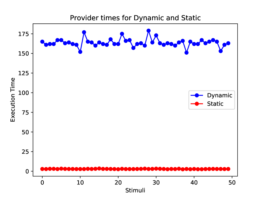
Figure 3: Comparison.

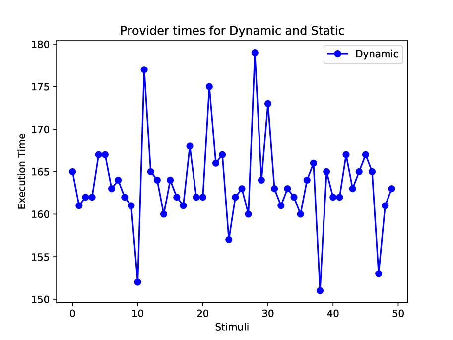
Figure 4: Zoom in Dynamic.

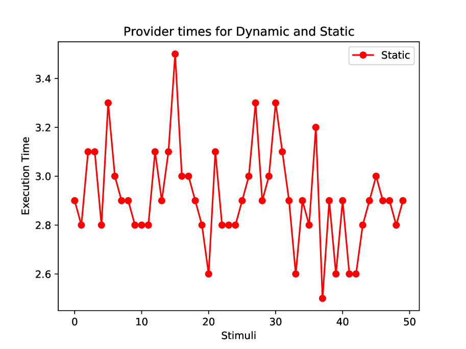
Figure 5: Zoom in Static.

It is an important detail that, since $\pi$ only provides ranges of inputs (e.g., a general $x|(x<2)$ instead of a concrete $x:1$), the input values may be different in both experiments. Therefore, we executed again the experiments over a same fixed input trace $\pi^{\prime}=(\langle x:4\rangle,\langle x:4\rangle,\langle x:1\rangle,\langle x:0\rangle,\langle x:2\rangle,\ldots)$ in order to do a sanity check. Fig. 8 shows that the execution with $\pi^{\prime}$ follows the same tendency as with $\pi$. Even though the input numbers are repeated, we still encounter differences in solving times both in Fig. 8 and Fig. 8, which suggests that, for such an amount of constraints to solve, the time to solve is not dominated by the input, but rather by implementation and memory details.

Figure 6: Comparison.

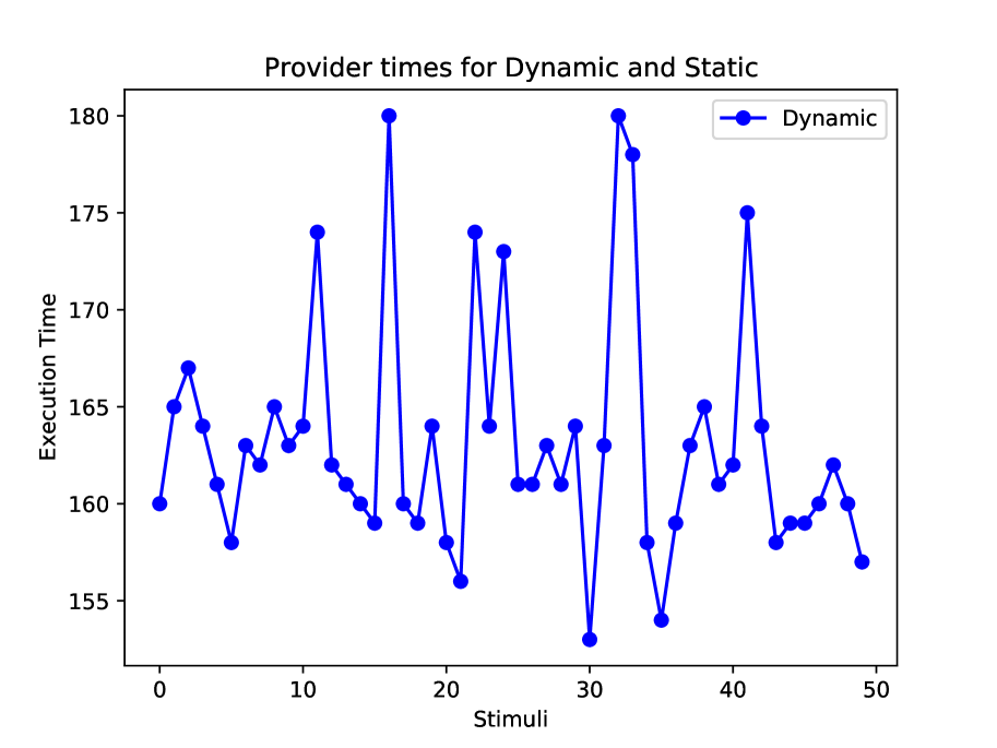
Figure 7: Zoom in Dynamic.

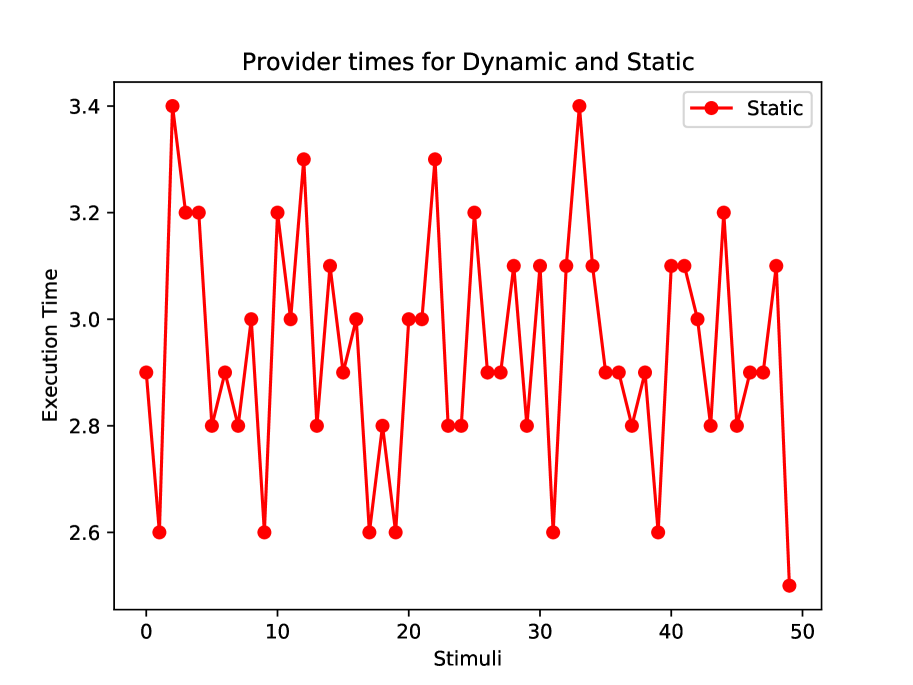
Figure 8: Zoom in Static.

We also checked the predictability of both approaches using $\pi^{\prime}$: i.e., how much does the output differ given the same input and position in the game. Recall from Ex. 2 and $\pi^{\prime}$ that at timestep $t:0$ the possible outcomes are $v_{\overline{y}}\in\{2,3,4\}$, at $t:1$ again $v_{\overline{y}}\in\{2,3,4\}$, at $t:2$ $v_{\overline{y}}\in\{2,3,4,...\}$, at $t:3$ again $v_{\overline{y}}\in\{2,3,4,...\}$ and at $t:4$ $v_{\overline{y}}\in\{2\}$. Let us denote with $k$ the repetition of this pattern. At time $t:0+k$ and $t:1+k$ there are three valid outputs, at $t:2+k$ and $t:3+k$ there are infinitely many valid outputs and at $t:4+k$ there is a single valid output. Also, note that $v_{\overline{y}}$ should be a valid output for every input in $\pi^{\prime}$ (as captured by both Skolem functions in Ex. 3). In Fig. 11, we show results for $500$ timesteps ($100\times|\pi^{\prime}|$). We can see that the dynamic $\<provider>$ is less predictable (outputs), whereas the static $\<provider>$ always produces the value $2$. Note that output values in the dynamic $\<provider>$ are always different in every experiment, but the general shape remains similar. Also, note that one might consider that predictability in the dynamic approach is also remarkably stable, since only for $20$ times out of the total of $400$ the $\<provider>$ produces a value different than $2$ ($17$ times value $3$, twice the value $4$ and once value $5$).

However, this stability difference increases when adaptivity is considered. Concretely, we will use return the greatest (illustrated in Ex. 5) for $t:0+k$, $t:1+k$ and $t:0+4$, and return the smallest for $t:2+k$ and $t:3+k$, which means that the ideal output trace with respect to these criteria is the pattern $(\langle y:4\rangle,\langle y:4\rangle,\langle y:2\rangle,\langle y:2\rangle,\langle y:2\rangle)$. As expected, the static $\<provider>$ always returns the ideal pattern, whereas the pattern in the dynamic case is more unstable. For example, in Fig. 11, we show results for $50$ stimuli in $\pi^{\prime}$, where three times the output was not within the ideal pattern. We acknowledge that, in the dynamic approach, as the timeout restrictions for the underlying SMT solver gets more strict (e.g., in fast embedded contexts), less adaptive constraints will be solved and thus the output will tend to diverge more from the ideal pattern.

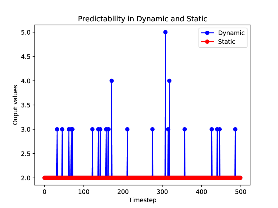
Figure 9: Comparison.

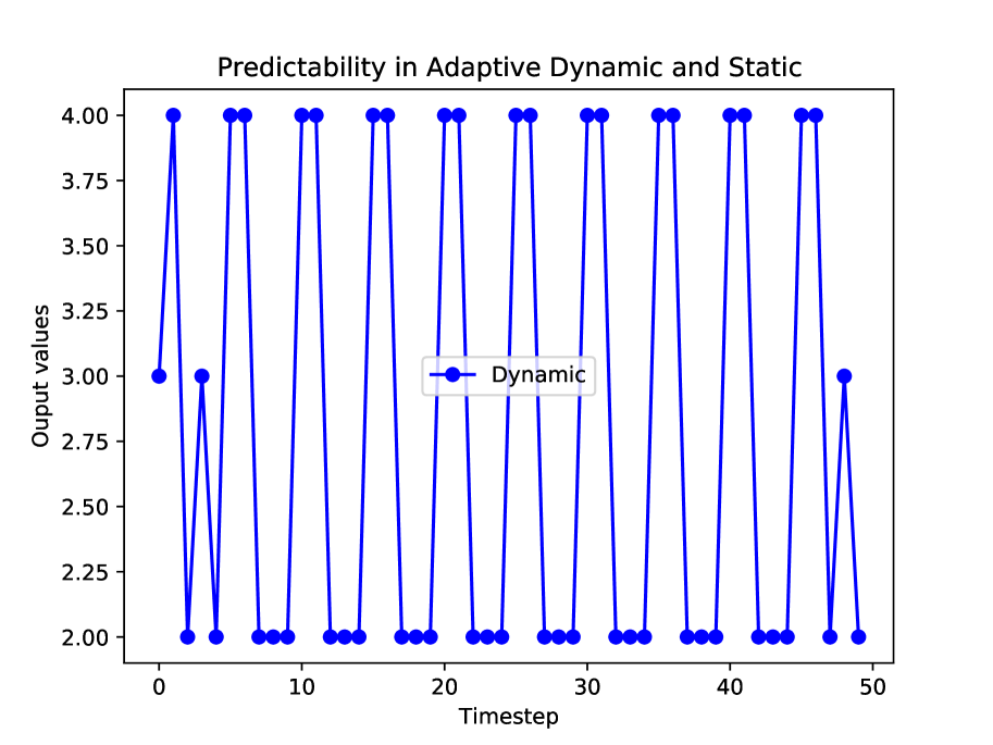
Figure 10: Dyn. Adaptive.

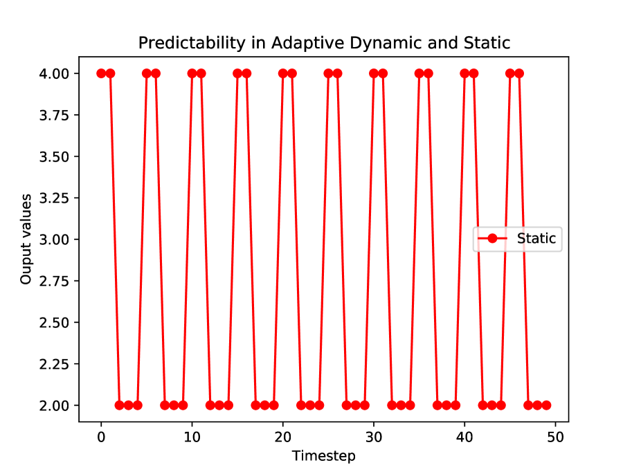
Figure 11: Static Adaptive.

5.0.2 Benchmark results.

In order to perform a wide empirical evaluation, we used benchmarks from [36] to validate the hypothesis whether that our static approach is faster and more predictable. Tab. 1 shows the main group of experiments. Sz. refers to the size of the $\varphi^{\mathcal{T}}$ specification both in variables (vr.) and literals (lt.). Prep. refers to the pre-processing time (i.e., the time needed to compute the Boolean abstraction and synthetize a Boolean controller). This and the computation of the $\<partitioner>$ are performed at compile time, while in our experiments $\<provider>$ is computed dynamically for each new $(v_{\overline{e}},v_{\overline{s}})$ pair discovered. Note that the time necessary to compute Skolem functions was negligible (around $2$ seconds) as expected, since the number of constraints we used does not stress AEval . The following two groups of columns show results of the execution of $1000$ ($1$K) and $10000$ ($10$K) timesteps of input-output simulations. For each group we do not show the average time that the $\<partitioner>$ takes to respond with a discrete $v_{\overline{e}}$ from $v_{\overline{x}}$ and the average time that the Boolean controller takes to respond with a Boolean $c_{i}$, since it is the same for the dynamic and the static approaches. Instead, we report the time that the $\<provider>$ takes to respond with a valuation associated to $c_{i}$ in dynamic (Dyn.) and static (St.). Note that Tr. is also the benchmark that takes the most time on average for Pr., since its functions contain more operations, but it is still efficient enough for the targeted applications. Overall, we can see that the static approach is $50$ to $60$ times faster.

In addition, we used adaptivity with different criteria. We selected Skolem functions of each benchmark and created adaptive versions that return: (1) minimum and maximum valuation possible (m/m) knowing there was at least one of such bounds to stop the search and (2) valuation closest to a $p$ point (pc.) that is randomly generated. Then, groups ($10$K (m/m)) and ($10$K (pc.)) measure again average times of the dynamic $\<provider>$ and adaptive $\<provider>$. Note that it is not clear how adaptivity impacts $\<provider>$ time, since sometimes the amount of adaptive constraints dominates this time, whereas in other cases the complexity of the criteria (e.g., underlying quantified structure) seems to be more relevant.

Bn.	Sz.	Prep.	$1K$		$10K$			$10K$ ($\textit{m/m.})$			$10K$ (pc.)
(nm.)	(vr, lt)	(s.)	Dyn.	St.	Dyn.	St.	Pre.	Dyn.	St.	Pre.	Dyn.	St.	Pre.
Li.	(5, 16)	33.73	240	5.74	232	4.54	$\sim 4$	216	4.01	$\sim 4$	204	3.52	$\sim 7$
Tr.	(19, 36)	9219.11	272	5.05	262	5.03	$\sim 9$	294	5.08	$\sim 14$	270	4.92	$\sim 15$
Con.	(2, 2)	0.09	104	2.08	104	1.89	$\sim 2$	107	1.94	$\sim 2$	129	2.18	$\sim 2$
Coo.	(3, 5)	2.60	171	2.94	168	2.84	$\sim 3$	168	3.32	$\sim 4$	173	2.81	$\sim 3$
Usb	(5, 8)	346.29	302	6.04	304	4.82	$\sim 5$	329	5.46	$\sim 7$	313	6.00	$\sim 6$
Sta.	(11, 14)	182.1	295	4.91	291	5.19	$\sim 6$	299	5.24	$\sim 9$	298	4.73	$\sim 11$

Table 1: Results in [36] (see Dyn.) versus ours (see St.), where times are measured in $\mu$. Recall from [35] that if the literals in $\varphi$ are split into clusters that do not share variables, the Boolean abstraction process can handle each cluster independently and composed afterwards.

Moreover, we show approximated predictability (Pre.) results of the dynamic approach as a percentage that measures how many of the outputs diverged from the ideal pattern (e.g., we previously mentioned that in Fig. 11 this number was $\sim 5\%$: $20$ divergences out of $400$ stimuli). In Tab. 1 we can see that predictability is between $2$ and $15$ percent (average about $5\%$), whereas in the static varsion it is $0\%$ (not shown in the table). More importantly, it seems that adding adaptivity tends to result in less predictable outputs in the dynamic $\<provider>$. These results support our hypothesis that our static controller is more efficient and predictable.

We also tested whether $\mathcal{T}$ affected the performance of the controller, via use cases Syn. (2,3) to Syn. (2,6) of [35] interpreted over linear integer arithmetic and linear real arithmetic (the theories accepted by AEval).

Lits	Linear I. Arithmetic			Linear R. Arithmetic
	1K (bs.)	1K (m/m)	1K (pc.)	1K (bs.)	1K (m/m)	1K (pc.)
$3$	$3.41$	$2.32$	$2.00$	$3.45$	$2.14$	$2.02$
$4$	$3.50$	$2.05$	$2.07$	$198$	$3.60$	$2.09$
$5$	$3.63$	$2.64$	$2.63$	$3.83$	$2.65$	$2.67$
$6$	$3.78$	$3.30$	$3.38$	$3.85$	$3.39$	$3.45$

Figure 12: Comparison of $\mathcal{T}_{\mathbb{Z}}$ and $\mathcal{T}_{\mathbb{R}}$ for Syn (2,3) to Syn (2,6).

We show the results in Fig. 12, where we compare $1000$ simulations in the basic case (bs.), and the adaptive minimal/maximal (m/m.) and randomly generated point (pc.) cases. Note that run-time difference is negligible and so was in the abstraction phase. Also, note that Skolem function synthesis was slightly harder in integers.

6 Related Work and Conclusions

6.0.1 Related Work.

LTL modulo theories has been previously studied (e.g., [23, 14]), but allowing temporal operators within predicates, again leading to undecidability. Also, infinite-state synthesis has been recently studied at [8, 15, 19, 39, 3, 24] but with similar restrictions. At [26, 27] authors perform reactive synthesis based on a fixpoint of $\forall^{*}\exists^{*}$ formulae (for which they use AEval), but expressivity is limited to safety and does not guarantee termination. The work in [41] also relies on abstraction but needs guidance and again expressivity is limited. Reactive synthesis of Temporal Stream Logic (TSL) modulo theories [18] is studied in [9, 28], which extends LTL with complex data that can be related accross time. Again, note that general synthesis is undecidable by relating values across time. Moreover, TSL is already undecidable for safety, the theory of equality and Presburger arithmetic. Thus, all the specifications considered for empirical evaluation in Sec. 5 are not within the considered decidable fragments.

All approaches above adapt one specific technique and implement it in a monolithic way, whereas [35, 37] generates LTL specification that existing tools can process with any of their internal algorithms (bounded synthesis, for example) so we will automatically benefit from further optimizations in these techniques. Moreover, Boolean abstraction preserves the temporal fragments like safety and GR(1) so specialized solvers can be used. Throughout the paper, we have already extensively compared the work [36] with ours and we showed that our approach uses Skolem functions instead of SMT queries on-the-fly, which makes it faster, more predictable and a pure controller that can be used in embedded contexts. It is worth noting that [36] and our approach can be understood as computing minterms to produce Symbolic automata and transducers [11, 12] from reactive specifications (and using antichain-based optimization, as suggested by [40]). Also, note that any advance in abstraction method (e.g., [4]) has an immediate positive impact in our work.

Last, [25] presents a similar idea to our Skolem function synthesis: instead of solving a quantified formula every time one wants to compute an output, they synthesize a term that computes the output from the input. However, the paper is framed in the program synthesis problem and uses syntax-guided synthesis [2], whereas previous reactive synthesis papers have suggested functional synthesis as a recommended software engineering practise (e.g., [38]).

6.0.2 Conclusion.

The main contribution of this paper is the synthesis procedure for $\textup{LTL}^{\mathcal{T}}$, using internally a Boolean controller and static Skolem function synthesis, which is more performant and predictable than previous approaches. Our method also allows producing adaptive responses that optimize the behaviour of the controller with respect to different criteria. We showed empirically that our approach is fast for many targeted applications and analyzed the cost and predictability of our Skolem functions component compared to [36]. As far as we know, this is the first decidable full reactive synthesis approach (with or with adaptivity) for $\textup{LTL}^{\mathcal{T}}$ specifications.

Future work includes first to use winning regions instead of concrete controllers to allow even more choices for the Skolem functions, and to develop a further adaptivity theory. Another direction is studying adaptivity over the environment inputs and combining this approach with monitoring. Also, we plan to study how to extend $\textup{LTL}^{\mathcal{T}}$ with transfer of data accross time preserving decidability, since recent results [22] suggest that the expressivity can be extended with limited transfers in semantic fragments of $\textup{LTL}^{\mathcal{T}}$. Moreover, explaining our synthesis approach within more general frameworks like (e.g., [21]) is immediate work to do. Finally, we want to study how to use our approach to construct more predictable and performant shields [1, 6] (concretely, shields modulo theories [34, 10]) to enforce safety in critical systems.

Appendix 0.A Complete running example

In $\varphi^{\mathcal{T}}$ of Ex. 1 a valid (positional) strategy of the system is to always play $y:2$. In this appendix we show that a controller synthetised using our technique will, precisely, respond in this manner infinitely many often. To do so, we rely on the trace of Ex. 2 and Skolem functions of Ex. 3.

First, we Booleanize $\varphi^{\mathcal{T}}$ using [35] and get $\varphi^{\mathbb{B}}$ (also, recall from Ex. 1 that we use the notation $c_{i}$ to indicate choice $i$; e.g., $c_{0}=\{s_{0},s_{1},s_{2}\}$, $c_{1}=\{s_{0},s_{1}\}$, …, $c_{6}=\{s_{2}\}$, $c_{7}=\emptyset$.). Then, we get a controller $C_{\mathbb{B}}$ from $\varphi^{\mathbb{B}}$. We note that many strategies satisfy $\varphi^{\mathbb{B}}$, but $C_{\mathbb{B}}$ by Strix is as follows: $C_{\mathbb{B}}(e_{1})=c_{4}$ and $C_{\mathbb{B}}(e_{0})=c_{1}$. Also, note that this particular strategy is memoryless, but there are diverse strategies that use memory. We now show how the static $\mathcal{T}$-controller computes Skolem functions on demand.

0.A.0.1 Step 1: Environment forces instant response.

Let $x:4$, which holds $(x\geq 2)$ and forces constraint $(y\leq x)$. We are in partition $e_{1}$, which implies choices $\{c_{4},c_{5},c_{6}\}$. Now, $C_{\mathbb{B}}(e_{1})=c_{4}$, so the $\mathcal{T}$-controller looks whether the pair $(e_{1},c_{1})$ appeared before. Since it did not, it computes $\mathtt{h}_{(e_{1},c_{4})}$ (see left-hand function at Ex. 3). Thus, $\mathtt{h}_{(e_{1},c_{4})}(2)=2$ is the output $v_{y}$ in the first timestep. Note that a $\mathcal{T}$-controller with a different underlying $C_{\mathbb{B}}$ could also consider $c_{6}$ in the current play.

0.A.0.2 Step 2: Environment repeats the strategy.

Again, $x:4$ and again we are in partition $e_{1}$. Now, $C_{\mathbb{B}}(e_{1})=c_{4}$, so the $\mathcal{T}$-controller looks whether the pair $(e_{1},c_{4})$ appeared before. Since it does, it just calls pre-computed $\mathtt{h}_{(e_{1},c_{4})}$. Thus, $\mathtt{h}_{(e_{1},c_{4})}(2)=2$ is the output $v_{y}$ in the second timestep.

0.A.0.3 Step 3: Environment changes its mind.

Let $x:1$, which holds $(x<2)$ and forces constraint $\LTLcircle(y>1)$, whereas no constraint is further for the current timestep. We are in partition $e_{0}$, which implies choices $\{c_{1},c_{2}\}$. Now, $C_{\mathbb{B}}(e_{0})=c_{1}$, so the $\mathcal{T}$-controller looks whether the pair $(e_{0},c_{1})$ appeared before. Since it did not, it computes $\mathtt{h}_{(e_{0},c_{1})}$ (see right-hand function at Ex. 3). Thus, $\mathtt{h}_{(e_{0},c_{1})}(2)=2$ is the output $v_{y}$ in the third timestep. Note that a $\mathcal{T}$-controller with a different underlying $C_{\mathbb{B}}$ could also consider $c_{2}$ in the current play.

0.A.0.4 Step 4: Environment prepares its trap.

Let $x:0$, which holds $(x<2)$ and forces constraint $\LTLcircle(y>1)$, and take into account that the system has constraint $(y>1)$ forced by the previous timestep. We are again in partition $e_{0}$, which implies, again, choices $\{c_{1},c_{2}\}$. Now, $C_{\mathbb{B}}(e_{0})=c_{1}$, so the $\mathcal{T}$-controller looks whether the pair $(e_{0},c_{1})$ appeared before. Since it does, it just calls pre-computed $\mathtt{h}_{(e_{0},c_{1})}$. Thus, $\mathtt{h}_{(e_{0},c_{1})}(2)=2$ is the output $v_{y}$ in the fourth timestep. Note that this time there is no correct $C_{\mathbb{B}}$ that could also consider $c_{2}$ in the current play.

0.A.0.5 Step 5: Environment strikes back!

Let $x:2$, which holds $(x\geq 2)$ and forces constraint $(y\leq x)$. Also, note that the system has constraint $(y>1)$ from previous timestep. We are in partition $e_{1}$, which implies choices $\{c_{4},c_{5},c_{6}\}$. Now, the same as in step 2 happens: $C_{\mathbb{B}}(e_{1})=c_{4}$, so the $\mathcal{T}$-controller looks whether the pair $(e_{1},c_{4})$ appeared before. Since it does, it just calls pre-computed $\mathtt{h}_{(e_{1},c_{4})}$. Thus, $\mathtt{h}_{(e_{1},c_{4})}(2)=2$ is the output $v_{y}$ in the fifth timestep.

Note that this is the dangerous situation, where the system can only output $y:2$; in other words, it happens again that there is no correct $C_{\mathbb{B}}$ that could also consider another choice (in this case, $c_{4}$ and $c_{5}$) in the current play. We can derive all the possible behaviours from these steps. Also, note that another possibility is to pre-compute all the Skolem functions, but it is less efficient.

Appendix 0.B More About Adaptivity

We outline several immediate consequences of using adaptivity of Sec. 4.

0.B.0.1 Across-time Adaptivity.

In the previous section we showed that if we can synthesize Skolem functions for adaptive provider formulae, then the system obtained is still a good system for the $\varphi^{\mathcal{T}}$. We show now that the additional arguments can be used to produce better controllers for $\varphi^{\mathcal{T}}$. For instance, $\overline{z}$ (thus, $v_{\overline{z}}$ in Fig. 2) can be used to feed past values to the controller, and $\psi^{+}$ can describe desired evolution of the output in terms of the past history.

Definition 8 (Across-time adaptive controller)

Let $\varphi^{\mathcal{T}}(\overline{x},\overline{y})$ be a specification, let $\Gamma$ be an adaptive provider description, and let $\rho^{\mathcal{T}}_{\Gamma}$ be the resulting controller. Then, we say that $\rho^{\mathcal{T}}_{\Gamma}$ is an across-time adaptive controller if the extra variables $\overline{z}$ in $\Gamma$ fed are past values of $\overline{x}$ and $\overline{y}$.

Example 6

Consider again the characteristic formula $\psi=(y>x)$, and the corresponding basic provider formula $\forall x.\exists y.\psi$, which is valid in $\mathcal{T}_{\mathbb{Z}}$. The constraint $\psi^{+}=(y>z)$ makes the adaptive provider formula $\varphi=\forall x,z.\exists y.(\psi\wedge\psi^{+})$ valid. A Skolem function $\mathtt{h}(x,z)$ guarantess that the output $y$ generated is greater than the values of both $x$ and $z$. Then, if the controller received $z$ as the value of $y$ in the previous timestep (denoted $y^{Y}$), then we have that the controller will generate outputs that are monotonically increasing.

Note that time adaptivity is not always possible. For example, using the constraint $\psi^{+}_{2}=(y<z)$ (which would force the output to be monotonically decreasing) would turn the resulting adaptive provider formula invalid, so a controller cannot be produced.

The practical implication of Def. 8 is that we can now produce controllers that in practice satisfy constraints that were not expressible in $\textup{LTL}^{\mathcal{T}}$ before, because the transfer of values across time quickly leads to undecidability of the realizability problem. Note that the Booleanization process in Sec. 3 only considers $\textup{LTL}^{\mathcal{T}}$ specifications where literals do not relate variables from different time instants (also called non-cross state fragment in [22]). Note that across-time adaptivity can be also used feeding to $\overline{z}$ the result of evaluating functions like average, historyMax on past values of $\overline{x}$ and $\overline{y}$.

As another example, a $\<provider>$ that is only required to keep $y$ within limits $[0,0.3]$ may choose any value within the bounds with a fixed Skolem function. However, the designer may prefer to choose “smooth” values that do not change dramatically to avoid abrupt changes in the values of $y$ (see Fig. 13). Therefore,

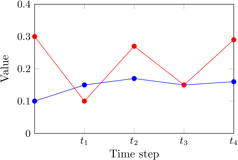
Figure 13: Abrupt vs. desired

instead of synthetising a basic function $f(x)$ for the valid formula $\forall x.\exists y.(0\leq y\leq 3)$, the controller will produce another $f(x)^{\text{smooth}}$ function for the valid formula $\forall x,y^{Y}.\exists y.(0\leq y\leq 3)\wedge\neg\exists w.[((0\leq z\leq 3))\wedge(|w-y^{Y}|<|y-y^{Y}|)]$, so that produced value for $y$ is as close as possible to value of $y$ in the previous timestep. Since the function exists, then the enriched specification will produce the desired controller that spans out of $\textup{LTL}^{\mathcal{T}}$. Note that the constraint $\psi^{+}$ in the previous example uses an additional quantifier $\exists w$. We show next practical applications and how to cope with this inner quantifier.

0.B.0.2 Approximations and Neurosymbolic Control.

Skolem functions computed from basic provider formulae have a shape $\forall^{*}\exists^{*}.\psi$. This shape is preserved in adaptive provider formulae in which the constraint $\psi^{+}$ is quantifier-free. However, as the last example illustrated, the constraint $\psi^{+}$ may include quantifiers, which does not preserve the shape typically amenable for Skolemization.

For instance, to compute the smallest $y\in\mathbb{D}(\mathcal{T}_{\mathbb{Z}})$ in $\forall x.\exists y.(y>x)$, one can use the adaptive provider formula $\forall x.\exists y.[(y>x)\wedge\forall z.(z>x)\mathrel{\rightarrow}(z\geq{}y)]$. We overcome this issue by performing quantifier elimination (QE) for the innermost quantifier and recover the $\forall^{*}\exists^{*}$ shape. In consequence, our resulting method works on any theory $\mathcal{T}$ that:

1. is decidable for the $\exists^{*}\forall^{*}$ fragment (for the Boolean abstraction);

2. permits a Skolem function synthesis procedure (for valid $\forall^{*}\exists^{*}$ formulae), for producing static providers; and

3. accepts QE (which preserves formula equivalence) for the flexibility in defining quentified constraints $\psi^{+}$.

The use of quantification opens the door to explore solutions that exploit characteristics of concrete theories. Consider for example the theory of Presburger arithmetic $\mathcal{T}_{\mathbb{Z}}$ (which we illustrate with single variable but can be extended to other notions of distance with multiple variables, such as Euclidean distance). In this theory the following holds.

Lemma 2 (Closest element)

In $\mathcal{T}_{\mathbb{Z}}$ the following holds. Assuming $\forall\overline{x}.\exists y.\psi(\overline{x},y)$, the following is also valid:

$$\forall\overline{x}.z.\exists y.\big{(}\psi(\overline{x},y)\mathrel{\wedge}\forall w.[\psi(\overline{x},w)\mathrel{\rightarrow}|y-z|\leq|w-z|]).$$

In other words, in $\mathcal{T}_{\mathbb{Z}}$ if for all inputs $\overline{x}$ there is an output $y$ such that $\psi$ holds, then there is always a closest value to any provided $z$ that satisfies $\psi$. The method we propose uses QE to provide a quantifier-free formula equivalent to $\psi^{+}=\forall w.[\psi(\overline{x},w)\mathrel{\rightarrow}|y-z|\leq|w-z|])$. The formula generated by the elimination depends on each specific constraint. Note that this formula only has $\overline{x}$, $z$ and $y$ as free variables. As a result the Skolem function generation will produce a function $\mathtt{h}(\overline{x},z)$ such that, given values for $\overline{x}$ and $z$, will provide an appropriate output (for $y$) that satisfies $\psi$ and is minimal (as expressed by the constraint $\psi^{+}$).

The following holds in $\mathcal{T}_{\mathbb{Z}}$, which essentially states that if the candidate $z$ satisfies $\psi$ then $\mathtt{h}$ will return it, and that $\mathtt{h}$ always returns a value satisfies $\psi$ and that is as close to $z$ as possible.

Proposition 1

Let $\psi(v_{\overline{x}},y)$ be valid and let $\mathtt{h}$ be a Skolem function of

$$\forall\overline{x}.z.\exists y.\big{(}\psi(\overline{x},y)\mathrel{\wedge}\forall w.[\psi(\overline{x},w)\mathrel{\rightarrow}|y-z|\leq|w-z|]).$$

Let $v_{\overline{x}}\in\mathit{val}(\overline{x})$ and $v_{z}\in\mathit{val}(z)$ be arbitrary value, and let $v_{y}=\mathtt{h}(v_{\overline{x}},v_{z})$. Then,

• If $\psi(v_{\overline{x}},v_{z})$ then $v_{y}=v_{z}$.

• Let $o$ be such that $\psi(v_{\overline{x}},o)$. Then $|v_{z}-v_{y}|\leq|v_{z}-o|$.

The theory of real arithmetic $\mathcal{T}_{\mathbb{R}}$ is also widely used, but unfortunately the equivalent of Lemma 2 does not hold because it may not be possible to find a value that satisfies $\psi$ and is the closest to a given candidate. However, it is always possible to compute a closest within a given tolerance given by a real constant $\epsilon$. This is expressed in the following lemma.

Lemma 3 (Approximately Closest Element)

In $\mathcal{T}_{\mathbb{R}}$ the following holds. Assuming $\forall\overline{x}.\exists y.\psi(\overline{x},y)$, then for every constant $\epsilon>0$, the following is valid:

$$\forall\overline{x}.z.\exists y.\big{(}\psi(\overline{x},y)\mathrel{\wedge}\forall w.[\psi(\overline{x},w)\mathrel{\rightarrow}|y-z|\leq|w-z|+\epsilon]).$$

Note that there is a practical alternative to using a constant $\epsilon$ (provided by the user), which consists of iteratively generating Skolem functions for increasingly better results, by starting from $\forall x.\exists z.\exists y.\psi(x,y)$ and refining to better Skolem functions with respect to e.g., closest $y$, such that, at every iteration, the resulting provider guarantees $\varphi^{\mathcal{T}}$.

Lemmas 2 and 3 allow computing adaptive controllers that guarantee $\varphi^{\mathcal{T}}$ and approximate the value provided externally to the controller. A very interesting possibility is to use an external program, e.g., computed using machine-learning (ML), that provides $v_{\overline{z}}$ of Fig. 2. We call neurosymbolic reactive synthesis to this combination of ML and adaptive controller synthesis. In this manner, we combine a correct-by-construction technique (the reactive synthesis modulo theories presented here) with a richer but potentially incorrect program that is trained to optimize sophisticated goals. The result is a controller that produces safe outputs by approximating the values proposed by the unsafe ML controller. This approach resembles shielding [1] in the sense that our approach will also always produce safe outputs. However, in our approach the value chosen can be different to the proposed by the ML even if the value proposed is safe (for example, to also guarantee smoothness). A further exploration of applications of neurosymbolic synthesis is out of the scope of this paper.

References

- [1] Mohammed Alshiekh, Roderick Bloem, Rüdiger Ehlers, Bettina Könighofer, Scott Niekum, and Ufuk Topcu. Safe reinforcement learning via shielding. In Sheila A. McIlraith and Kilian Q. Weinberger, editors, Proc. of the Thirty-Second AAAI Conference on Artificial Intelligence, (AAAI-18), pages 2669–2678. AAAI Press, 2018.
- [2] Rajeev Alur, Rastislav Bodík, Garvit Juniwal, Milo M. K. Martin, Mukund Raghothaman, Sanjit A. Seshia, Rishabh Singh, Armando Solar-Lezama, Emina Torlak, and Abhishek Udupa. Syntax-guided synthesis. In Proc. of the 13th Int’l Conf. on Formal Methods in Computer-Aided Design (FMCAD 2013), pages 1–8. IEEE, 2013.
- [3] Shaun Azzopardi, Nir Piterman, Gerardo Schneider, and Luca di Stefano. Ltl synthesis on infinite-state arenas defined by programs, 2023.
- [4] Shaun Azzopardi, Nir Piterman, Gerardo Schneider, and Luca Di Stefano. LTL synthesis on infinite-state arenas defined by programs. CoRR, abs/2307.09776, 2023.
- [5] Roderick Bloem, Barbara Jobstmann, Nir Piterman, Amir Pnueli, and Yaniv Sa’ar. Synthesis of reactive(1) designs. J. Comput. Syst. Sci., 78(3):911–938, 2012.
- [6] Roderick Bloem, Bettina Könighofer, Robert Könighofer, and Chao Wang. Shield synthesis: - runtime enforcement for reactive systems. In Proc. of the 21st International Conference in Tools and Algorithms for the Construction and Analysis of Systems (TACAS 2015), volume 9035 of LNCS, pages 533–548. Springer, 2015.
- [7] Aaron R. Bradley and Zohar Manna. The Calculus of Computation. Springer-Verlag, 2007.
- [8] Chih-Hong Cheng and Edward A. Lee. Numerical LTL synthesis for cyber-physical systems. CoRR, abs/1307.3722, 2013.
- [9] Wonhyuk Choi, Bernd Finkbeiner, Ruzica Piskac, and Mark Santolucito. Can reactive synthesis and syntax-guided synthesis be friends? In Ranjit Jhala and Isil Dillig, editors, 43rd ACM SIGPLAN Int’l Conf. on Programming Language Design and Implementation (PLDI 2022), pages 229–243. ACM, 2022.
- [10] Davide Corsi, Guy Amir, Andoni Rodriguez, Cesar Sanchez, Guy Katz, and Roy Fox. Verification-guided shielding for deep reinforcement learning. CoRR, abs/2406.06507, 2024.
- [11] Loris D’Antoni and Margus Veanes. Minimization of symbolic automata. In Proc. of the 41st Annual ACM SIGPLAN-SIGACT Symposium on Principles of Programming Languages (POPL ’14), pages 541–554. ACM, 2014.
- [12] Loris D’Antoni and Margus Veanes. The power of symbolic automata and transducers. In Proc. of the 29th International Conference in Computer Aided Verification (CAV 2017), Part I, volume 10426 of LNCS, pages 47–67. Springer, 2017.
- [13] Leonardo de Moura and Nikolaj Bjørner. Z3: An efficient SMT solver. In Proc. of the 14th Int’l Conf. on Tools and Algorithms for the Construction and Analysis of Systems (TACAS’08), volume 4693 of LNCS, pages 337–340. Springer, 2008.
- [14] Rachel Faran and Orna Kupferman. LTL with arithmetic and its applications in reasoning about hierarchical systems. In Proc. of the 22nd International Conference on Logic for Programming, Artificial Intelligence and Reasoning, (LPAR-22. ), volume 57 of EPiC Series in Computing, pages 343–362. EasyChair, 2018.
- [15] Azadeh Farzan and Zachary Kincaid. Strategy synthesis for linear arithmetic games. Proc. ACM Program. Lang., 2(POPL):61:1–61:30, 2018.
- [16] Grigory Fedyukovich, Arie Gurfinkel, and Aarti Gupta. Lazy but effective functional synthesis. In 20th International Conference in Verification, Model Checking, and Abstract Interpretation, (VMCAI 2019), volume 11388 of LNCS, pages 92–113. Springer, 2019.
- [17] Bernd Finkbeiner. Synthesis of reactive systems. In Javier Esparza, Orna Grumberg, and Salomon Sickert, editors, Dependable Software Systems Engineering, volume 45 of NATO Science for Peace and Security Series - D: Information and Communication Security, pages 72–98. IOS Press, 2016.
- [18] Bernd Finkbeiner, Philippe Heim, and Noemi Passing. Temporal stream logic modulo theories. In 25th Int’l Conf. on Foundations of Software Science and Computation Structures (FOSSACS 2022), volume 13242 of LNCS, pages 325–346. Springer, 2022.
- [19] Andrew Gacek, Andreas Katis, Michael W. Whalen, John Backes, and Darren D. Cofer. Towards realizability checking of contracts using theories. In Proc. of the 7th International Symposium NASA Formal Methods (NFM 2015), volume 9058 of LNCS, pages 173–187. Springer, 2015.
- [20] Luca Geatti, Alessandro Gianola, and Nicola Gigante. Linear temporal logic modulo theories over finite traces. In Proc. of the 31st International Joint Conference on Artificial Intelligence, (IJCAI 2022), pages 2641–2647. ijcai.org, 2022.
- [21] Luca Geatti, Alessandro Gianola, and Nicola Gigante. A general automata model for first-order temporal logics (extended version). CoRR, abs/2405.20057, 2024.
- [22] Luca Geatti, Alessandro Gianola, Nicola Gigante, and Sarah Winkler. Decidable fragments of ltlf modulo theories (extended version). CoRR, abs/2307.16840, 2023.
- [23] Alessandro Gianola and Nicola Gigante. LTL modulo theories over finite traces: modeling, verification, open questions. In Short Paper Proceedings of the 4th Workshop on Artificial Intelligence and Formal Verification, Logic, Automata, and Synthesis hosted by the 21st International Conference of the Italian Association for Artificial Intelligence (AIxIA 2022), volume 3311 of CEUR Workshop Proceedings, pages 13–19. CEUR-WS.org, 2022.
- [24] Philippe Heim and Rayna Dimitrova. Solving infinite-state games via acceleration. Proc. ACM Program. Lang., 8(POPL):1696–1726, 2024.
- [25] Qinheping Hu and Loris D’Antoni. Automatic program inversion using symbolic transducers. In Proc. of the 38th ACM SIGPLAN Conference on Programming Language Design and Implementation (PLDI 2017), pages 376–389. ACM, 2017.
- [26] Andreas Katis, Grigory Fedyukovich, Andrew Gacek, John D. Backes, Arie Gurfinkel, and Michael W. Whalen. Synthesis from assume-guarantee contracts using skolemized proofs of realizability. CoRR, abs/1610.05867, 2016.
- [27] Andreas Katis, Grigory Fedyukovich, Huajun Guo, Andrew Gacek, John Backes, Arie Gurfinkel, and Michael W. Whalen. Validity-guided synthesis of reactive systems from assume-guarantee contracts. In Proc. of the 24th International Conference on Tools and Algorithms for the Construction and Analysis of Systems, (TACAS 2018), volume 10806 of LNCS, pages 176–193. Springer, 2018.
- [28] Benedikt Maderbacher and Roderick Bloem. Reactive synthesis modulo theories using abstraction refinement. In 22nd Formal Methods in Computer-Aided Design, (FMCAD 2022), pages 315–324. IEEE, 2022.
- [29] Zohar Manna and Amir Pnueli. Temporal verification of reactive systems - safety. Springer, 1995.
- [30] Philipp J. Meyer, Salomon Sickert, and Michael Luttenberger. Strix: Explicit reactive synthesis strikes back! In Hana Chockler and Georg Weissenbacher, editors, Computer Aided Verification, pages 578–586, Cham, 2018. Springer International Publishing.
- [31] Amir Pnueli. The temporal logic of programs. In Proc. of the 18th IEEE Symp. on Foundations of Computer Science (FOCS’77), pages 46–67. IEEE CS Press, 1977.
- [32] Amir Pnueli and Roni Rosner. On the synthesis of a reactive module. In Proc. of the 16th Annual ACM Symp. on Principles of Programming Languages (POPL’89), pages 179–190. ACM Press, 1989.
- [33] Amir Pnueli and Roni Rosner. On the synthesis of an asynchronous reactive module. In Proc. of the 16th Int’l Colloqium on Automata, Languages and Programming (ICALP’89), volume 372 of LNCS, pages 652–671. Springer, 1989.
- [34] Andoni Rodriguez, Guy Amir, Davide Corsi, Cesar Sanchez, and Guy Katz. Shield synthesis for LTL modulo theories. CoRR, abs/2406.04184, 2024.
- [35] Andoni Rodríguez and César Sánchez. Boolean Abstractions for Realizability Modulo Theories. In Proc. of the 35th Int’l Conf. on Computer Aided Verification (CAV 2023), volume 13966 of LNCS, pages 1–24. Springer, 2023.
- [36] Andoni Rodriguez and César Sánchez. Adaptive reactive synthesis for LTL and LTLf modulo theories. In Proc. of the 38th AAAI Conf. on Artificial Intelligence (AAAI 2024), pages 10679–10686. AAAI Press, 2024.
- [37] Andoni Rodriguez and César Sanchez. Realizability modulo theories. Journal of Logical and Algebraic Methods in Programming, page 100971, 2024.
- [38] Stanly Samuel, Deepak D’Souza, and Raghavan Komondoor. Gensys: a scalable fixed-point engine for maximal controller synthesis over infinite state spaces. In Proc. of the 29th ACM Joint European Software Engineering Conference and Symposium on the Foundations of Software Engineering (ESEC/FSE’21), pages 1585–1589. ACM, 2021.
- [39] Stanly Samuel, Deepak D’Souza, and Raghavan Komondoor. Symbolic fixpoint algorithms for logical LTL games. In Proc. of the 38th IEEE/ACM International Conference on Automated Software Engineering (ASE 2023), pages 698–709. IEEE, 2023.
- [40] Margus Veanes, Thomas Ball, Gabriel Ebner, and Olli Saarikivi. Symbolic automata: -regularity modulo theories. CoRR, abs/2310.02393, 2023.
- [41] Adam Walker and Leonid Ryzhyk. Predicate abstraction for reactive synthesis. In Proc. of the 14th Formal Methods in Computer-Aided Design, (FMCAD 2014), pages 219–226. IEEE, 2014.