All order factorization for virtual Compton scattering at next-to-leading power

Abstract

We discuss all-order factorization for the virtual Compton process at next-to-leading power (NLP) in the $\Lambda_{\rm QCD}/Q$ and $\sqrt{-t}/Q$ expansion (twist-3), both in the double-deeply-virtual case and the single-deeply-virtual case. We use the soft-collinear effective theory (SCET) as the main theoretical tool. We conclude that collinear factorization holds in the double-deeply virtual case, where both photons are far off-shell. The agreement is found with the known results for the hard matching coefficients at leading order $\alpha_{s}^{0}$, and we can therefore connect the traditional approach with SCET. In the single-deeply-virtual case, commonly called deeply virtual Compton scattering (DVCS), the contribution of non-target collinear regions complicates the factorization. These include momentum modes collinear to the real photon and ultrasoft interactions between the photon-collinear and target-collinear modes. Indeed, we identify a potentially problematic non-perturbative contribution, which might violate the universality of the generalized parton distributions (GPDs) at NLP accuracy.

1 Introduction

The GPDs  Muller:1994ses ; Ji:1996ek ; Ji:1996nm ; Radyushkin:1997ki have a rich physical interpretation in terms of transverse spatial probability distribution of partons with a given longitudinal momentum fraction Burkardt:2002hr and are essential for studying the decomposition of the proton spin Ji:1996ek and various inter- and multi-parton correlations inside the hadrons. GPD studies are subject to active research in nuclear and high-energy physics and have been stated as a significant science goal for the planned Electron-Ion collider at Brookhaven National Laboratory AbdulKhalek:2021gbh ; AbdulKhalek:2022hcn .

The deeply virtual Compton scattering (DVCS) Ji:1996ek ; Ji:1996nm is considered the “golden” channel for experimentally accessing GPDs. This process is defined as electroproduction of a real photon from the nucleon

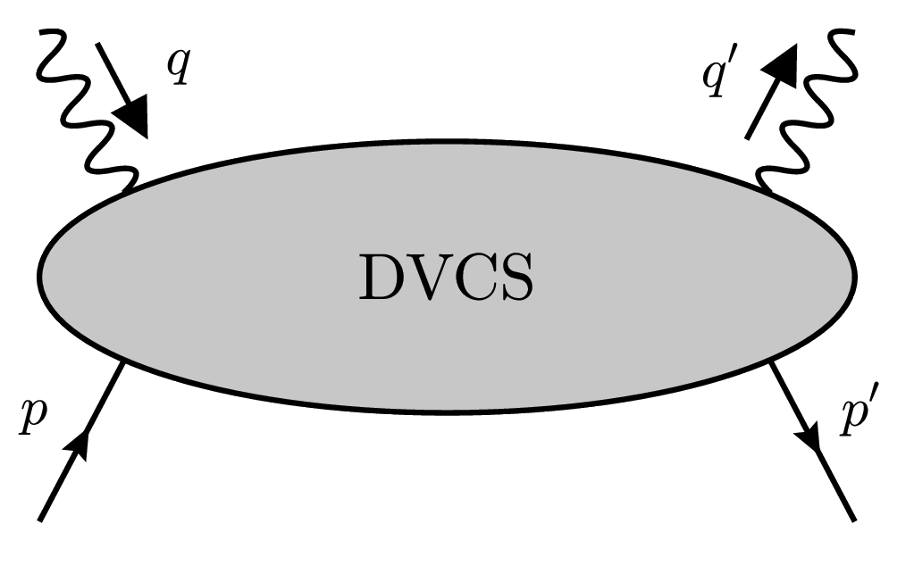
Figure 1: The DVCS process.

$$\gamma^{*}(q)+N(p)\rightarrow\gamma(q^{\prime})+N^{\prime}(p^{\prime}),$$ (1)

where $\gamma^{*}$ is the highly virtual photon exchanged between a lepton and the nucleon. Its virtuality $-q^{2}>0$ provides the hard scale of the processes, and it is assumed to be much larger than the scale of strong interactions $\Lambda_{\rm QCD}$. This strong scale separation allows for factorization of the short-distance hard physics contained in the coefficient functions and long-distance non-perturbative effects encoded in GPDs. The QCD input needed to describe DVCS is entirely encoded in the hadronic tensor

$$T^{\mu\nu}=i\int d^{4}z\,e^{-iq\cdot z}\bra{p^{\prime}}T\{j^{\mu}(z)j^{\nu}(0)\}\ket{p},$$ (2)

where $j^{\mu}=\sum_{q}e_{q}\bar{\psi}_{q}\gamma^{\mu}\psi_{q}$ is the electromagnetic current. Factorization and perturbative behavior of DVCS has been comprehensively understood at leading power: All-order factorization at $(\Lambda_{\rm QCD}/Q)^{0}$ has been proven in Radyushkin:1997ki ; Collins:1998be ; Ji:1998xh ; Bauer:2002nz and the coefficients function are known to the next-to-next-to-leading order $\alpha_{s}^{2}$ Braun:2022bpn ; Ji:2023xzk . A great deal is known beyond leading power due to the operator product expansion; for example, Braun:2012hq and the recent development Braun:2022qly .

In this work, we focus on next-to-leading power (NLP) effects, which are suppressed by $(\Lambda_{\rm QCD}/Q)^{1}$ compared to the leading power. At this accuracy, the DVCS amplitude has been hypothesized to factorize into twist-3 GPDs, which have a rich physical interpretation in themselves, see, e.g., Hatta:2012cs ; Hatta:2024otc . The corresponding leading $\alpha_{s}^{0}/Q$ coefficient functions have been known for a long time and even a part of the next-to-leading order $\alpha_{s}^{1}/Q$ contribution has been calculated in Kivel:2003jt . For a more recent discussion, see Aslan:2018zzk .

However, the all-order factorization of DVCS at NLP has never been discussed in the same level of detail as that of the leading power. The important subtleties that cast doubts about the factorization in its hypothesized form are due to non-target-collinear regions that arise when the outgoing photon becomes real, therefore introducing a second collinear direction. In particular, if the regions where partons become ultrasoft contribute to the power accuracy in question, one may expect endpoint-like divergences of the convolution integral of the hard coefficient functions with the non-perturbative objects. This usually implies that the IR singularities are not adequately factored into these non-perturbative objects. While this does not necessarily mean that factorization in the broad sense is broken (this can happen for example if Glauber regions are present), it might mean that there are additional contributions that require additional refactorization (see Liu:2019oav ; Beneke:2020ibj ; Hurth:2023paz and Beneke:2022obx ; Liu:2020wbn ; Liu:2020tzd ; Liu:2022ajh ; Beneke:2019kgv ; Cornella:2022ubo for related discussion). The observed absence of endpoint-like divergences in DVCS at NLP at tree-level Kivel:2000cn (and partly at one-loop Kivel:2003jt ) does indicate that factorization holds in its assumed form. Still, it provides by no means a level of confidence associated with established factorization analyses. Indeed, there is no reason to suppose that regions where partons become ultrasoft necessarily lead to endpoint-like divergences, even if they contribute to the power accuracy in question.

The soft-collinear effective theory (SCET) Bauer:2000yr ; Bauer:2001ct ; Bauer:2001yt ; Bauer:2002nz enables a systematic study of power corrections without appealing to the operator product expansion. In this work, we use the position space formulation Beneke:2002ph ; Beneke:2002ni . As substantiated by the method of regions analysis in section 3), the relevant physical infrared (IR) modes for DVCS are given by

$$n\text{-collinear}:\qquad p_{n}\sim(\lambda^{2},1,\lambda)Q,$$

$$\bar{n}\text{-collinear}:\qquad p_{\bar{n}}\sim(1,\lambda^{2},\lambda)Q,$$ (7)

$$\text{ultrasoft}:\qquad p_{s}\sim(\lambda^{2},\lambda^{2},\lambda^{2})Q.$$

Here $\lambda$ is a dimensionless power counting parameter that equals some fixed momentum scale, in this case either $\Lambda_{\rm QCD},\,m_{N}=\sqrt{p^{2}}=\sqrt{p^{\prime 2}}$ or $\sqrt{-t}=\sqrt{-(p-p^{\prime})^{2}}$, divided by $Q$. In other words, $\lambda\rightarrow 0$ parametrizes the limit $Q\rightarrow\infty$ with the different scales fixed. It is not necessary to further specify the definition of $\lambda$ unless one wants to investigate potentially large-scale ratios in certain kinematic limits such as $Q\gg\sqrt{-t}\gg\Lambda_{\rm QCD}$. This kinematic limit is also connected to the chiral and trace anomalies of QCD, which was subject to some recent work in the context of DVCS Bhattacharya:2022xxw ; Bhattacharya:2023wvy . We will not discuss such issues in this work and assume that all low energy scales are parametrically equal. We will see later that the chiral anomaly also plays an interesting role in the context of this work. Still, there is, at this point, no reason to assume that this is in any way related to the issues regarding the $Q\gg\sqrt{-t}\gg\Lambda_{\rm QCD}$ region.

We choose a frame such that the approximate direction of the in- and outgoing proton is along $n$ and the approximate direction of the outgoing photon is along $\bar{n}$. This means we will refer to the proton momentum as collinear and the outgoing photon as anti-collinear. In the modern effective field theory (EFT) approach, every momentum mode of a field that corresponds to a different scale is described by separate fields. The hard modes are integrated-out, and SCET contains only fields corresponding to collinear, anti-collinear, and ultrasoft modes:

$$\phi=\phi_{n}+\phi_{\bar{n}}+\phi_{s}\,.$$ (8)

The Lagrangian is subsequently expanded in $\lambda$, so each term has strictly homogeneous scaling in the expansion parameter. The resulting Lagrangian up to next-to-leading power and all corresponding definitions are collected in Appendix A.

One could ask whether the modes in eq. (7) are sufficient to fully describe the virtual Compton process at NLP accuracy. In the method of region analysis of the one-loop graph in section 3, the soft region $p_{s^{\prime}}\sim(\lambda,\lambda,\lambda)Q$ leads to a scaleless integral. It is not apparent that this is true to all orders, even if there is no explicit physical soft scale. For example, in Nabeebaccus:2023rzr , it was seen that the soft region played a role in a more complicated process. In such a case, the soft region seems to be relevant only in combination with the Glauber interactions, e.g., with momentum scaling $p_{G(sn)}\sim(\lambda,\lambda^{2},\lambda)Q$, which can occur between soft $p_{s^{\prime}}$ and $n$-collinear $p_{n}$ spectator lines. Another example of where the Glauber region presents a problem for collinear factorization in the context of GPD physics was identified in Braun:2002wu . The Glauber-like regions, where $\bar{n}\cdot p_{G}\,n\cdot p_{G}\ll p_{G\perp}^{2}$ are notoriously dangerous for factorization and their implementation in SCET, while well understood Rothstein:2016bsq , is complicated. However, it is a well-established Collins:2011zzd claim that a necessary condition for the Glauber pinch is the presence of at least two collinear external particles, which are in different collinear directions, in both the initial and final state (given that there are no soft external particles). Since the virtual Compton process can not meet this criterion, it is safe to assume that no Glauber pinch can occur.

So far, SCET has been applied to describe GPDs in a single work Bauer:2002nz , where only the leading power factorization is discussed. In this work, we extend the analysis to NLP. The arguments that require the most new development are needed to deal with the $\bar{n}$-collinear and ultrasoft modes that superficially contribute at NLP. In section 4.3, we will identify a non-perturbative contribution involving these modes, possibly breaking the universality of the GPD description of DVCS at NLP.

We start by analyzing a one-loop graph in section 3 and show that, for this example, the non-target collinear regions are next-to-next-to-leading power (NNLP). In section 4, we extend the analysis to all orders using SCET. In the subsection 4.3, we discuss the potentially problematic ultrasoft quark region, which seems to give a non-perturbative and non-universal contribution at NLP.

In section 5, we perform the tree-level matching, which is a straightforward exercise. Then, in section 6, we show that the SCET formulation reproduces the established result Kivel:2000cn in that it yields the same twist-3 GPDs with the same coefficient functions. In the literature, many different frames are used to describe DVCS. One can translate between the frames using reparametrization invariance (RPI) symmetry of SCET. We use the frame introduced in Braun:2012hq throughout most of this work, but we also convert to the frames of Kivel:2000cn and Belitsky:2005qn by using RPI in section 7.

Since it does not cost much effort, we simultaneously discuss the case where both photons are far off-shell, known as double-deeply virtual Compton scattering (DDVCS). However, we always have in mind the conceptually more riveting case of DVCS, where the outgoing photon is real.

2 Kinematics and reference frame

We use the following definitions

$$P^{\mu}=\frac{p^{\mu}+p^{\prime\mu}}{2},\qquad\Delta=p^{\prime}-p,\qquad Q^{2}=-\frac{1}{4}(q+q^{\prime})^{2},\qquad t=\Delta^{2}\,,$$ (9)

and we define

$$\rho =-\frac{(q+q^{\prime})^{2}}{4P\cdot(q+q^{\prime})}.$$ (10)

Note that $\rho$ reduces to $x_{B}=\frac{Q^{2}}{2p\cdot q}$ in the forward case $p=p^{\prime}$.

The skewness $\eta$ is defined as

$$\eta=-\frac{\Delta\cdot\bar{n}}{P\cdot\bar{n}}\,,$$ (11)

and is not a Lorentz-scalar since $\bar{n}^{\mu}$ is a fixed reference vector that does not transform under Lorentz transformations. Indeed, definitions of $\eta$ in the literature differ by $\mathcal{O}(\lambda^{2})$ terms. DVCS is obtained by taking $\rho=\eta$, as will be manifest from the explicit parametrization of the momenta below.

As mentioned, we always assume collinear scaling $p,p^{\prime},\Delta,P\sim(\lambda^{2},1,\lambda)Q$ and this implies that $1-\eta\sim\eta\sim 1$. Furthermore, we assume that $q^{\prime}\sim(1,\lambda^{2},\lambda)Q$ for DVCS. Various frames are used in the DVCS literature to satisfy these conditions. We consider the following three:

• The Compton frame $P_{\perp}=q_{\perp}+q_{\perp}^{\prime}=0$, which is used for example in Ji:1998xh and Belitsky:2005qn . We have

  $$\Delta_{\perp}^{2}=4m^{2}\eta^{2}+t(1-\eta^{2})\,,$$ (12)

  and

  $$p^{\mu} =(1+\eta)\bar{n}\cdot P\frac{n^{\mu}}{2}+(1-\eta)\frac{m^{2}-t/4}{\bar{n}\cdot P}\frac{\bar{n}^{\mu}}{2}-\frac{1}{2}\Delta_{\perp}^{\mu},$$

  $$p^{\prime\mu} =(1-\eta)\bar{n}\cdot P\frac{n^{\mu}}{2}+(1+\eta)\frac{m^{2}-t/4}{\bar{n}\cdot P}\frac{\bar{n}^{\mu}}{2}+\frac{1}{2}\Delta_{\perp}^{\mu},$$

  $$q^{\mu} =-(\rho+\eta)\bar{n}\cdot P\frac{n^{\mu}}{2}+\frac{Q^{2}}{\rho\bar{n}\cdot P}\frac{\bar{n}^{\mu}}{2}+\frac{1}{2}\Delta_{\perp}^{\mu}+\mathcal{O}\left(\frac{t}{Q},\frac{m^{2}}{Q}\right),$$ (13)

  $$q^{\prime\mu} =-(\rho-\eta)n\cdot P\frac{n^{\mu}}{2}+\frac{Q^{2}}{\rho\bar{n}\cdot P}\frac{\bar{n}^{\mu}}{2}-\frac{1}{2}\Delta_{\perp}^{\mu}+\mathcal{O}\left(\frac{t}{Q},\frac{m^{2}}{Q}\right).$$

• The Kivel-Polyakov (KP) frame, where $P_{\perp}=q_{\perp}=0$, adopted, for example, in Kivel:2000cn . We have

  $$\Delta_{\perp}^{2}=4m^{2}\eta^{2}+t(1-\eta^{2})\,,$$ (14)

  and

  $$p^{\mu} =(1+\eta)\bar{n}\cdot P\frac{n^{\mu}}{2}+(1-\eta)\frac{m^{2}-t/4}{\bar{n}\cdot P}\frac{\bar{n}^{\mu}}{2}-\frac{1}{2}\Delta_{\perp}^{\mu},$$

  $$p^{\prime\mu} =(1-\eta)\bar{n}\cdot P\frac{n^{\mu}}{2}+(1+\eta)\frac{m^{2}-t/4}{\bar{n}\cdot P}\frac{\bar{n}^{\mu}}{2}+\frac{1}{2}\Delta_{\perp}^{\mu},$$

  $$q^{\mu} =-(\rho+\eta)\bar{n}\cdot P\frac{n^{\mu}}{2}+\frac{Q^{2}}{\rho\bar{n}\cdot P}\frac{\bar{n}^{\mu}}{2}+\mathcal{O}\left(\frac{t}{Q},\frac{m^{2}}{Q}\right),$$ (15)

  $$q^{\prime\mu} =-(\rho-\eta)n\cdot P\frac{n^{\mu}}{2}+\frac{Q^{2}}{\rho\bar{n}\cdot P}\frac{\bar{n}^{\mu}}{2}-\Delta_{\perp}^{\mu}+\mathcal{O}\left(\frac{t}{Q},\frac{m^{2}}{Q}\right).$$

• The Braun-Manashov-Pirnay (BMP) frame Braun:2012hq , where $\Delta_{\perp}=q_{\perp}^{\prime}=0$. Then

  $$P_{\perp}^{2}=m^{2}+\frac{t}{4}\frac{1-\eta^{2}}{\eta^{2}}\,,$$ (16)

  and

  $$p^{\mu} =(1+\eta)\bar{n}\cdot P\frac{n^{\mu}}{2}+\frac{1-\eta}{4\eta^{2}}\frac{(-t)}{\bar{n}\cdot P}\frac{\bar{n}^{\mu}}{2}+P_{\perp}^{\mu},$$

  $$p^{\prime\mu} =(1-\eta)\bar{n}\cdot P\frac{n^{\mu}}{2}+\frac{1+\eta}{4\eta^{2}}\frac{(-t)}{\bar{n}\cdot P}\frac{\bar{n}^{\mu}}{2}+P_{\perp}^{\mu},$$

  $$q^{\mu} =-(\rho+\eta)\bar{n}\cdot P\frac{n^{\mu}}{2}+\frac{Q^{2}}{\rho\bar{n}\cdot P}\frac{\bar{n}^{\mu}}{2}+\mathcal{O}\left(\frac{t}{Q},\frac{m^{2}}{Q}\right),$$ (17)

  $$q^{\prime\mu} =-(\rho-\eta)\bar{n}\cdot P\frac{n^{\mu}}{2}+\frac{Q^{2}}{\rho\bar{n}\cdot P}\frac{\bar{n}^{\mu}}{2}.$$

We will use almost exclusively the BMP frame, which is convenient since the photons have vanishing $\perp$ momentum at NLP accuracy. In the case of DVCS, $q^{\prime}$ is exactly a light-like vector.

Our derivation relies on the choice of the BMP frame, more precisely, on the condition $q_{\perp}^{\prime}=0$. Then, given that the number and virtuality of momentum regions is a Lorentz invariant Pecjak:2005uh , we conclude that if factorization holds in one frame, it also holds in another, at least as long as the scaling of the external momenta is left invariant. Furthermore, using the reparametrization invariance (RPI) Manohar:2002fd ; Chay:2002vy of the amplitude, which represents the residual Lorentz symmetry in SCET, we can convert a factorized expression from one frame to another. This is done in section 7.

3 Method of regions example

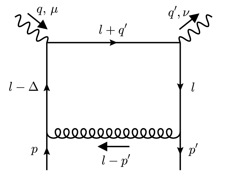
Figure 2: Box diagram with DVCS kinematics.

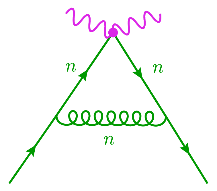
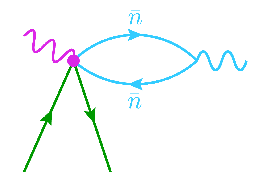
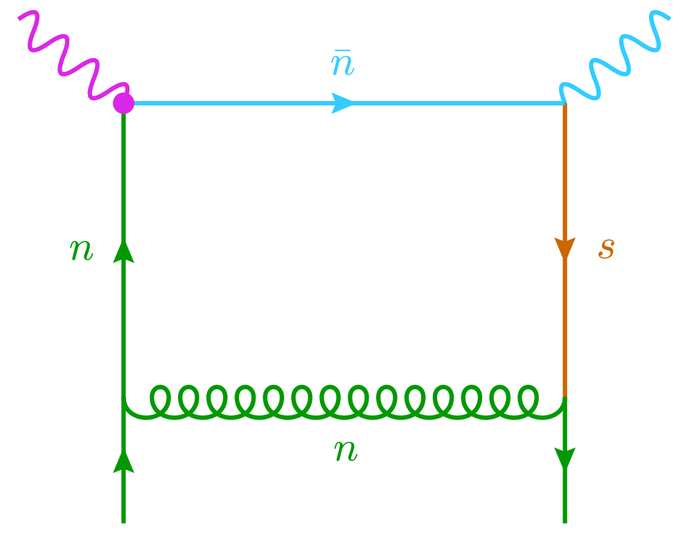
(a)                             (b)                                                      (c)

Figure 3: Reduced diagrams of figure 2 corresponding to the regions in eq. (7).

It is instructive to start with a “simple” example to substantiate the all-order arguments made later. We employ the method of regions Beneke:1997zp , i.e., we assume various scalings of loop momentum with expansion parameter $\lambda$, perform expansion of the integrand in $\lambda$, integrate over the entire range. The sum of all the regions represents the expansion of the integral in $\lambda$.

This section aims to check whether the only relevant IR region is the $n$-collinear region and all other IR regions are beyond our $\mathcal{O}(\lambda^{1})$-accuracy. This statement is straightforward if both photons are far off-shell. Below, we consider the more interesting case of DVCS, i.e. $\rho=\eta$. We will find that for this one-loop loop example, it is indeed true that only the $n$-collinear region contributes to NLP accuracy.

We consider the box diagram in figure 2, which reads (ignoring the trivial color algebra)

$$I^{\mu\nu} =\int d^{4}l\,\frac{\bar{u}(p^{\prime})\gamma_{\alpha}\not{l}\gamma^{\nu}(\not{l}+\not{q}^{\prime})\gamma^{\mu}(\not{l}-\not{\Delta})\gamma^{\alpha}u(p)}{[(l+q^{\prime})^{2}+i0][(l-\Delta)^{2}+i0][l^{2}+i0][(l-p^{\prime})^{2}+i0]}.$$ (18)

To get homogeneous in $\lambda$ integrand, we need to expand the spinor $u(p)$ in terms of the collinear spinor $u_{n}(p)=\frac{\not{n}\not{\bar{n}}}{4}u(p)$. Using the Dirac equation $\not{p}u(p)=0$, we get

$$u(p)-u_{n}(p)=\frac{\not{\bar{n}}\not{n}}{4}u(p)=-\frac{\not{\bar{n}}\not{p}_{\perp}}{2\bar{n}\cdot p}u_{n}(p),$$ (19)

so we have

$$u(p)=\left(1-\frac{\not{\bar{n}}\not{p}_{\perp}}{2\bar{n}\cdot p}\right)u_{n}(p),\qquad\bar{u}(p^{\prime})=\bar{u}_{n}(p^{\prime})\left(1-\frac{\not{p}_{\perp}^{\prime}\not{\bar{n}}}{2\bar{n}\cdot p^{\prime}}\right).$$ (20)

These relations are also critical in the matching procedure discussed in section 5.

First, the soft region $l\sim(\lambda,\lambda,\lambda)Q$ gives a scaleless integral, which vanishes in dimensional regularization. The hard region is trivially present and gives the bare contribution to the one-loop coefficient functions. Let us recall that $\Delta,p,p^{\prime}\sim p_{n}$ and $q^{\prime}\sim p_{\bar{n}}$ and:

• Start with the $n$-collinear region: $l\sim(\lambda^{2},1,\lambda)Q$. The reduced diagram is shown in figure 3(a):

  $$n\text{-collinear}:\qquad I_{n}\sim\underbrace{\lambda^{4}}_{\text{mom. space volume}}\,\underbrace{\lambda^{2}}_{\text{ numerator }}\,\underbrace{\lambda^{-6}}_{\text{denominator}}\sim\lambda^{0}.$$ (21)

  To see this, we note that each collinear denominator, except for the first one, gives a power of $\lambda^{-2}$. In the numerator, note that $\bar{u}(p^{\prime})\gamma_{\perp\alpha}\not{n},\;\not{n}\gamma_{\perp}^{\alpha}u(p)\sim\lambda$, so the large component of $\not{l}$ and $\not{l}-\not{\Delta}$ contributes only with suppressed spinor components. On the other hand, for $\not{l}+\not{q}^{\prime}$, we can pick the $n\cdot q^{\prime}\frac{\not{\bar{n}}}{2}$ component, which scales as $\lambda^{0}$. Notice that in this region, we can replace, up to terms of $\mathcal{O}(\lambda^{2})$,

  $$\frac{\not{l}+\not{q}^{\prime}}{(l+q^{\prime})^{2}+i0}\longrightarrow\frac{1}{\bar{n}\cdot l+i0}\left(\frac{\not{\bar{n}}}{2}+\frac{\not{l}_{\perp}}{n\cdot q^{\prime}}\right)\;.$$ (22)

  To get the factorization of the graph in the usual language, we would write $\bar{n}\cdot l=(x-\eta)\bar{n}\cdot P$. The first term in the brackets on the righthand side of eq. (22) is then nothing but the contribution to the leading order coefficient function $\frac{1}{x-\eta+i0}$. The second term in the bracket contributes to the coefficient function of a twist-3 operator.

• Continue with the $\bar{n}$-collinear region: $l\sim(1,\lambda^{2},\lambda)Q$. Notice that in the strictly on-shell limit, this region leads to a scaleless integral because $q^{\prime 2}=0$, i.e., there is no physical scale in the process corresponding to anti-collinear virtuality. Instead, let us consider the photon slightly of-shell $q^{\prime 2}\sim\lambda^{2}Q$ by introducing a non-zero $\lambda^{2}Q\sim\bar{n}\cdot q^{\prime}\neq 0$. This off-shellness can be physically related to the breakdown of perturbative expansion below scale $\Lambda_{\rm QCD}$ for anti-collinear matrix elements and experimentally it can be thought of as a finite energy resolution of the photon detector. The reduced diagram is shown in figure 3(b). Superficially:

  $$\bar{n}-\text{collinear}:\quad I_{\bar{n}}\sim\underbrace{\lambda^{4}}_{\text{mom. space volume}}\,\underbrace{\lambda^{0}}_{\text{ numerator }}\,\underbrace{\lambda^{-4}}_{\text{denominator}}\sim\lambda^{0}.$$ (23)

  The power-counting for the numerator requires some explanation. In particular, it depends heavily on the polarization of photons. The largest term responsible for the leading power behavior is obtained by taking the $\not{n}$ components of $\gamma^{\nu}$ and $\gamma^{\mu}$. Then, we can take the $\not{\bar{n}}$ component of $\not{l},\not{l}+\not{q}^{\prime},\not{l}-\not{\Delta}$, giving the leading power. However, this contributes only to the unphysical longitudinal polarization of the outgoing photon. For physical photon polarization, we can effectively replace $\gamma^{\nu}\rightarrow\gamma_{\perp}^{\nu}$. Let us assume this from now on. In the $\bar{n}$-collinear region up to terms of $\mathcal{O}(\lambda^{2})$ the integral can be written as

  $$I_{\bar{n}}=\frac{\bar{n}^{\mu}}{\bar{n}\cdot\Delta\,\bar{n}\cdot p^{\prime}}\int d^{4}l\,\frac{\bar{u}_{n}\gamma_{\perp\alpha}\Big{[}\not{l}_{\perp}\gamma_{\perp}^{\nu}n\cdot(l+q^{\prime})n\cdot l\frac{\not{\bar{n}}}{2}+n\cdot l\frac{\not{\bar{n}}}{2}\gamma_{\perp}^{\nu}\not{l}_{\perp}\Big{]}n\cdot l\gamma_{\perp}^{\alpha}u_{n}}{[(l+q^{\prime})^{2}+i0](l^{2}+i0)(n\cdot l+i0)(n\cdot l-i0)}.$$ (24)

  Now, it is clear that $I_{\bar{n}}$ is proportional to $q_{\perp}^{\prime\nu}=0$, so $I_{\bar{n}}$ vanishes. We conclude that the $\bar{n}$-collinear region is $\mathcal{O}(\lambda^{2})$.

• Finally, consider the ultrasoft region $l\sim p_{s}$. The reduced diagram is shown in figure 3(c). Superficially:

  $$\text{ultrasoft}:\quad I_{s}\sim\underbrace{\lambda^{8}}_{\text{mom. space volume}}\,\underbrace{\lambda^{3}}_{\text{ numerator }}\,\underbrace{\lambda^{-10}}_{\text{denominator}}\sim\lambda^{1}.$$ (25)

  The integral in the ultrasoft region can be written as

  $$I_{s}=\int d^{4}l\,\frac{\bar{u}_{n}\gamma_{\perp\alpha}\not{l}_{\perp}\gamma_{\perp}^{\nu}n\cdot q^{\prime}\frac{\not{\bar{n}}}{2}\gamma^{\mu}\bar{n}\cdot\Delta\frac{\not{n}}{2}\gamma_{\perp}^{\alpha}\frac{\not{\bar{n}}\not{P}_{\perp}}{2\bar{n}\cdot p}u_{n}}{[n\cdot q^{\prime}\,\bar{n}\cdot l+q^{\prime 2}+i0][-\bar{n}\cdot\Delta\,n\cdot l+\Delta^{2}+i0][-\bar{n}\cdot p^{\prime}n\cdot l+p^{\prime 2}+i0](l^{2}+i0)}$$ (26)

  Notice that we can drop $l_{\perp}$ in each denominator, except for $l^{2}+i0$. Thus the $l_{\perp}$ integral is odd under $l_{\perp}\rightarrow-l_{\perp}$, so we get zero. Consequently, the ultrasoft region is $\mathcal{O}(\lambda^{2})$.

Strictly speaking, one also has to take into account the overlap contributions as formulated in Jantzen:2011nz . However, it is easy to see that these give scaleless integrals.

We conclude that as long as the real photon is transversely polarized and $q_{\perp}^{\prime}=0$, the only relevant non-hard contribution to $I$ at NLP is the $n$-collinear contribution. We will find that the operatorial expansion in the SCET framework readily generalizes these arguments to all graphs and all orders. However, we will see that the argument used to conclude that the ultrasoft region vanishes relies on chiral symmetry, which is spontaneously broken by non-perturbative effects. To intuitively understand this complication for our example, we can consider introducing a fictitious mass $M\sim\Lambda_{\rm QCD}$ by taking $\not{l}_{\perp}\rightarrow\not{l}_{\perp}+M$ in the numerator in eq. (26). Then, $I_{s}\sim\lambda$ is proportional to $M$ and non-zero.

4 All-order factorization

4.1 Operator building blocks

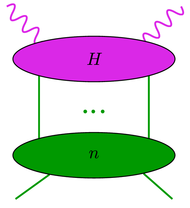
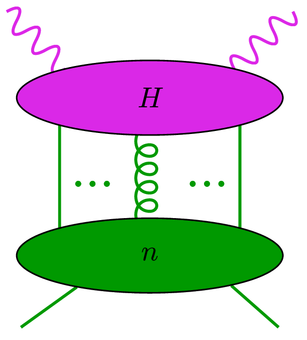
(a)                                          (b)

Figure 4: All-order reduced diagrams involving only $n$-collinear regions. The dots denote an arbitrary number of scalar-polarized gluons. The quark lines connecting the hard and $n$-collinear subgraph can also be transversely polarized gluon lines. The right-hand diagram (b) contains an additional transversely polarized gluon connecting the hard and $n$-collinear subgraph, corresponding to an NLP correction.

This section relies on the definitions introduced in Appendix A. To derive factorization using the EFT formalism, we first have to identify all gauge-invariant operators, and we can use reparametrization invariance to constrain the operator basis.

Collinear gauge invariance is automatically satisfied by the introduction of collinear gauge invariant collinear building blocks:

$$\begin{array}[]{ll}\displaystyle\chi_{n}(x)=W_{n}^{\dagger}(x)\xi_{n}(x)\sim\lambda^{1}&{\quad{\text{$n$-collinear quark,}}}\\[8.5359pt] \displaystyle\mathcal{A}^{\mu}_{{n}\perp}(x)=W_{n}^{\dagger}(x)\big{[}iD^{\mu}_{{n}\perp}W_{n}(x)\big{]}\sim\lambda^{1}&{\quad{\text{$n$-collinear gluon,}}}\end{array}$$ (27)

which are composed of the $n$-collinear fields before the ultrasoft decoupling transformation

$$\xi_{n}\rightarrow Y_{n}^{[n]}\xi_{n},\qquad A_{n}\rightarrow Y_{n}^{[n]}A_{n}Y_{n}^{[n]\dagger}.$$ (28)

Further, the subleading gluon building block $n\cdot\mathcal{A}_{{n}}(x)=W_{n}^{\dagger}(x)\big{[}n\cdot iD_{{n}}W_{n}(x)\big{]}$, can be eliminated using equation of motion Beneke:2017ztn . The collinear building blocks can be acted upon with derivative operators

$$\partial_{\perp}\sim\lambda^{1},\qquad n\cdot D_{s}\sim\lambda^{2},$$ (29)

where, due to the multipole expansion of the ultrasoft fields, only the $n\cdot D_{s}$ has to be a ultrasoft gauge covariant derivative rather than an ordinary derivative. This derivative operator can also be eliminated from operator basis Beneke:2017ztn ; Beneke:2019kgv .

In addition, the operators may contain ultrasoft building blocks

$$\begin{array}[]{ll}\displaystyle q_{s}(0)\sim\lambda^{3}&{\quad{\text{soft quark,}}}\\[8.5359pt] \displaystyle F_{s}^{\mu\nu}(0)\sim\lambda^{4}&{\quad{\text{soft gluon,}}}\end{array}$$ (30)

which only start contributing from relative $\mathcal{O}(\lambda^{3})$ order Beneke:2017ztn . The ultrasoft gauge invariance of a generic operator is equivalent to the color neutrality of the entire operator.

After the ultrasoft decoupling transformation, the operators may contain the ultrasoft Wilson lines that sum up the unsuppressed interactions of scalar-polarized ultrasoft gluons with the collinear fields. If we consider an operator containing only $n$-collinear building blocks (understood to be evaluated on the $\bar{n}$-light-cone) sourced by a color singlet, the ultrasoft Wilson lines cancel.

4.2 Target-only collinear modes

Let us focus only on operators constructed from $n$-collinear building blocks. The leading power operators that have non-zero overlap with the off-forward hadron matrix element $\bra{p^{\prime}}...\ket{p}$ contain two building blocks.

$$\mathcal{O}_{\bar{\chi}\chi}^{[\Gamma]}(s_{1},s_{2})=\bar{\chi}_{n}(s_{1}\bar{n})\frac{\Gamma}{2}\chi_{n}(s_{2}\bar{n}),\qquad\mathcal{O}_{\mathcal{A}\mathcal{A}}^{\mu_{1}\mu_{2}}(s_{1},s_{2})=\text{tr}(\mathcal{A}_{n\perp}^{\mu_{1}}(s_{1}\bar{n})\mathcal{A}_{n\perp}^{\mu_{2}}(s_{2}\bar{n})).$$ (31)

As usual, the SCET operators are non-local along the lightcone. The hadronic matrix element of these operators can be identified with the lower $n$-collinear subgraph of the reduced graph figure 4(a). As for the basis of Dirac matrices one conventionally chooses $\Gamma\in\{\not{\bar{n}},\not{\bar{n}}\gamma_{5},\sigma^{\mu\nu}_{~{}\,\perp}\bar{n}_{\mu}\}$. We do not decompose the Lorentz indices of the operators $\mathcal{O}_{\mathcal{A}\mathcal{A}}^{\mu_{1}\mu_{2}}$ since gluons do not appear at leading order in $\alpha_{s}$ and we will only consider $\alpha_{s}^{0}$ matching. We only note that there exist three possible tensor structures; see Ji:2023xzk for the general decomposition in $d$ dimensions.

The next-to-leading power color-singlet operators are

$$\mathcal{O}_{\bar{\chi}\partial\chi}^{[\Gamma]\mu}(s_{1},s_{2}) =\bar{\chi}_{n}(s_{1}\bar{n})\frac{\Gamma}{2}i\overleftrightarrow{\partial}_{\perp}^{\mu}\chi_{n}(s_{2}\bar{n}),$$

$$\mathcal{O}_{\partial(\bar{\chi}\chi)}^{[\Gamma]\mu}(s_{1},s_{2}) =i\partial_{\perp}^{\mu}(\bar{\chi}_{n}(s_{1}\bar{n})\frac{\Gamma}{2}\chi_{n}(s_{2}\bar{n})),$$

$$\mathcal{O}_{\bar{\chi}\mathcal{A}\chi}^{[\Gamma]\mu}(s_{1},s_{2},s_{3}) =\bar{\chi}_{n}(s_{1}\bar{n})\frac{\Gamma}{2}\mathcal{A}_{n\perp}^{\mu}(s_{2}\bar{n})\chi_{n}(s_{3}\bar{n}),$$

$$\mathcal{O}_{\mathcal{A}\partial\mathcal{A}}^{\mu_{1}\mu_{2}\mu_{3}}(s_{1},s_{2}) =\text{tr}(\mathcal{A}_{n\perp}^{\mu_{1}}(s_{1}\bar{n})i\overleftrightarrow{\partial}_{\perp}^{\mu_{2}}\mathcal{A}_{n\perp}^{\mu_{3}}(s_{2}\bar{n})),$$ (32)

$$\mathcal{O}_{\partial(\mathcal{A}\mathcal{A})}^{\mu_{1}\mu_{2}\mu_{3}}(s_{1},s_{2}) =\partial_{\perp}^{\mu_{1}}\text{tr}(\mathcal{A}_{n\perp}^{\mu_{2}}(s_{1}\bar{n})\mathcal{A}_{n\perp}^{\mu_{3}}(s_{2}\bar{n})),$$

$$\mathcal{O}_{\mathcal{A}\mathcal{A}\mathcal{A}}^{\mu_{1}\mu_{2}\mu_{3}}(s_{1},s_{2},s_{3}) =\text{tr}(\mathcal{A}_{n\perp}^{\mu_{1}}(s_{1}\bar{n})\mathcal{A}_{n\perp}^{\mu_{2}}(s_{2}\bar{n})\mathcal{A}_{n\perp}^{\mu_{3}}(s_{3}\bar{n})).$$

Note that $\mathcal{O}_{\bar{\chi}\partial\chi}$ and $\mathcal{O}_{\partial(\bar{\chi}\chi)}$ correspond to the reduced graph in figure 4(a), where we keep the $\mathcal{O}(\lambda^{1})$ term of the hard subgraph. On the other hand, the tri-local operators correspond to the reduced graph in figure 4(b). It can be readily checked that the SCET power-counting agrees with the graphical counting rules Collins:2011zzd , upon noting that the external hadron collinear states count for $\lambda^{-1}$ each.

Note that $\mathcal{O}_{\partial(\bar{\chi}\chi)}^{[\Gamma]\mu}$ and $\mathcal{O}_{\partial(\mathcal{A}\mathcal{A})}^{[\Gamma]\mu}$ are trivially related to leading power operators, e.g.

$$\bra{p^{\prime}}\mathcal{O}_{\partial(\bar{\chi}\chi)}^{[\Gamma]\mu}\ket{p}=\bra{p^{\prime}}\left[-i{\rm P}_{\perp}^{\mu},\mathcal{O}_{\bar{\chi}\chi}^{[\Gamma]}\right]\ket{p}=-i\Delta_{\perp}^{\mu}\bra{p^{\prime}}\mathcal{O}_{\bar{\chi}\chi}^{[\Gamma]\mu}\ket{p},$$ (33)

where ${\rm P}_{\perp}^{\mu}$ is the momentum operator. In the BMP frame, these operators do not contribute.

To define parton density functions, it is first convenient to eliminate one of the positions by a translational invariance in the collinear sector. The (SCET) parton densities are then defined as Fourier-transformed matrix elements with respect to the relative light-cone positions $s_{i}$. We use the following convention for bi-local operators:

$$\bra{p^{\prime}}\mathcal{O}_{\bar{\chi}\chi}^{[\Gamma]}(-s/2,s/2)\ket{p} =\bar{n}\cdot P\int_{-\infty}^{\infty}dx\,e^{-ixs\bar{n}\cdot P}F_{\bar{\chi}\chi}^{[\Gamma]}(x),$$ (34)

$$\bra{p^{\prime}}\mathcal{O}_{\bar{\chi}\partial\chi}^{[\Gamma]\mu}(-s/2,s/2)\ket{p} =(\bar{n}\cdot P)^{2}\int_{-\infty}^{\infty}dx\,e^{-ixs\bar{n}\cdot P}F_{\bar{\chi}\partial\chi}^{[\Gamma]\mu}(x).$$ (35)

In addition to momentum fraction $x$, the GPDs depend implicitly on $\eta,t$ and the factorization scale $\mu_{F}$. This dependence is tacitly implied and will be omitted from notation throughout.

For the quark-gluon-quark operator, we define

$$\bra{p^{\prime}}\mathcal{O}_{\bar{\chi}\mathcal{A}\chi}^{[\Gamma]\mu}(-s_{1}/2,s_{2}/2,s_{1}/2)\ket{p}$$

$$=(\bar{n}\cdot P)^{2}\int_{-\infty}^{\infty}dx_{1}dx_{2}\,e^{-ix_{1}s_{1}\bar{n}\cdot P-ix_{2}s_{2}\bar{n}\cdot P}F_{\bar{\chi}\mathcal{A}\chi}^{[\Gamma]\mu}(x_{1},x_{2})$$ (36)

and similarly for the other tri-local operators.

If the operators in eqs. (31) and (32) are indeed sufficient at NLP, the factorization follows immediately

$$T^{\mu\nu} =\sum_{\ell}\int_{-\infty}^{\infty}\frac{ds}{2\pi}\,\hat{C}_{\ell}^{\mu\nu}(s)\bra{p^{\prime}}\mathcal{O}_{\ell}(-s/2,s/2)\ket{p}$$

$$\quad+\sum_{\ell}\int_{-\infty}^{\infty}ds_{1}ds_{2}\,\hat{C}_{\ell}^{\mu\nu}(s_{1},s_{2})\bra{p^{\prime}}\mathcal{O}_{\ell}(-s_{1}/2,s_{2}/2,s_{1}/2)\ket{p}+\mathcal{O}(\lambda^{2}),$$ (37)

where $\ell$ is a multiindex that runs over all operators eqs. (31) and (32). In terms of the Fourier transformed coefficient functions

$$C_{\ell}^{\mu\nu}(x) =(\bar{n}\cdot P)^{\text{dim}\,\mathcal{O}_{\ell}-2}\int_{-\infty}^{\infty}\frac{ds}{2\pi}\,\hat{C}_{\ell}^{\mu\nu}(s)e^{-ixs\bar{n}\cdot P},$$

$$C_{\ell}^{\mu\nu}(x_{1},x_{2}) =(\bar{n}\cdot P)^{\text{dim}\,\mathcal{O}_{\ell}-2}\int_{-\infty}^{\infty}ds_{1}ds_{2}\,\hat{C}_{\ell}^{\mu\nu}(s_{1},s_{2})e^{-ix_{1}s_{1}\bar{n}\cdot P-ix_{2}s_{2}\bar{n}\cdot P},$$ (38)

the factorization theorem reads

$$T^{\mu\nu}=\sum_{\ell}\int_{-\infty}^{\infty}dx\,C_{\ell}(x)F_{\ell}(x)+\sum_{\ell}\int_{-\infty}^{\infty}dx_{1}dx_{2}\,C_{\ell}(x_{1},x_{2})F_{\ell}(x_{1},x_{2})+\mathcal{O}(\lambda^{2}).$$ (39)

This factorization applies without caveats if both photons have hard virtualities. In that case, no $\bar{n}$-collinear modes contribute, and any ultrasoft interactions are absent.

We remark that for light-cone distributions like the $F_{\ell}$’s one can Jaffe:1983hp ; Diehl:1998sm typically drop the time-ordering prescription in the matrix elements and assume compact support, supposedly contained in the region $-1\leq x_{j}\leq 1$. Assuming this remains true in SCET, one can limit the range of integration in eq. (39) to $-1\leq x_{j}\leq 1$, but we will never use this property.

4.3 Ultrasoft and $\bar{n}$-collinear contributions

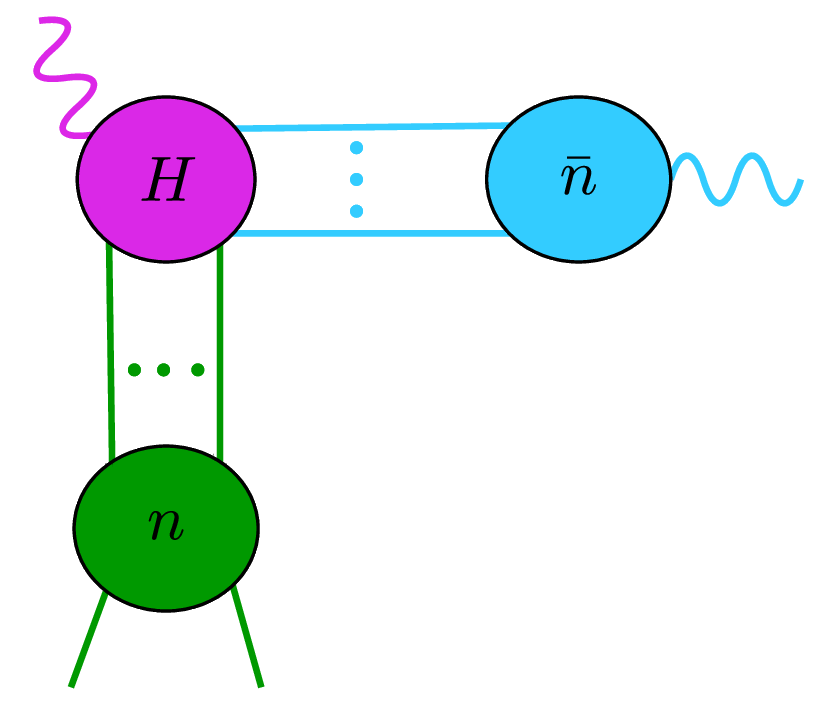
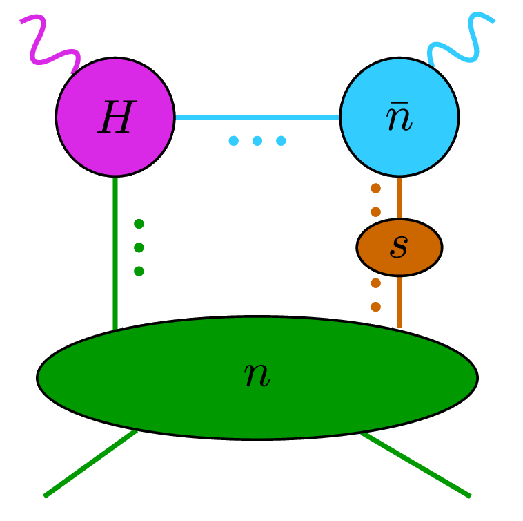
(a)                                                                        (b)

Figure 5: Reduced diagrams that involve $\bar{n}$-collinear and ultrasoft regions. The dots denote an arbitrary number of scalar-polarized gluons.

When one photon is on-shell, and therefore light-like, say in the $\bar{n}$-collinear direction, we have to take into account $\mathcal{L}_{\bar{n}}^{(0)}$ and ultrasoft interactions, which are due to the subleading SCET Lagrangians $\mathcal{L}_{ns}^{(1)}$ and $\mathcal{L}_{\bar{n}s}^{(1)}$. For definiteness, we consider the case where the outgoing photon is on-shell $\rho=\eta$, but the arguments apply similarly to the case where the incoming photon is on-shell $\rho=-\eta$.

We first need to identify the QED interaction terms (in terms of SCET fields) that can mediate the emission of the real photon. We strictly work to leading order in the electromagnetic coupling, so we always consider the external photon amputated and the polarization vector implicitly contracted with the index $\nu$. After the ultrasoft decoupling transformation eq  (28), the corresponding interaction vertices in SCET are given by

$$\mathcal{T}_{\bar{n}\bar{n}}^{\nu} =i\int d^{4}z\,\bar{\xi}_{\bar{n}}\frac{\not{n}}{2}\Big{[}\bar{n}^{\nu}e^{iq^{\prime}\cdot z}+i\not{D}_{\bar{n}\perp}\frac{1}{in\cdot D_{\bar{n}}}\gamma_{\perp}^{\nu}e^{iq^{\prime}\cdot z}+\gamma_{\perp}^{\nu}e^{iq^{\prime}\cdot z}\frac{1}{in\cdot D_{\bar{n}}}i\not{D}_{\bar{n}\perp}$$

$$\hskip 65.44142pt-i\not{D}_{\bar{n}\perp}\frac{1}{in\cdot D_{\bar{n}}}n^{\nu}e^{iq^{\prime}\cdot z}\frac{1}{in\cdot D_{\bar{n}}}i\not{D}_{\bar{n}\perp}\Big{]}\xi_{\bar{n}},$$ (40)

$$\mathcal{T}_{\bar{n}s}^{\nu} =i\int d^{4}z\,\left[\bar{q}_{s}^{[\bar{n}]}Y_{\bar{n}}^{[\bar{n}]}\gamma^{\nu}e^{iq^{\prime}\cdot z}\chi_{\bar{n}}+\bar{\chi}_{\bar{n}}\gamma^{\nu}e^{iq^{\prime}\cdot z}Y_{\bar{n}}^{[\bar{n}]}q_{s}^{[\bar{n}]}\right].$$ (41)

Note that the components of $\mathcal{T}_{\bar{n}\bar{n}}^{\nu}$ are not all of the same size because we amputated the photon field. In fact

$$n\cdot\mathcal{T}_{\bar{n}\bar{n}} =i\int d^{4}z\,\bar{\xi}_{\bar{n}}\not{n}e^{iq^{\prime}\cdot z}\xi_{\bar{n}}\sim\lambda^{-2},$$

$$\mathcal{T}_{\bar{n}\bar{n}\perp}^{\nu} =i\int d^{4}z\,\bar{\xi}_{\bar{n}}\frac{\not{n}}{2}\left[i\not{D}_{\bar{n}\perp}\frac{1}{in\cdot D_{\bar{n}}}\gamma_{\perp}^{\nu}e^{iq^{\prime}\cdot z}+\gamma_{\perp}^{\nu}e^{iq^{\prime}\cdot z}\frac{1}{in\cdot D_{\bar{n}}}i\not{D}_{\bar{n}\perp}\right]\xi_{\bar{n}}\sim\lambda^{-1},$$ (42)

$$\bar{n}\cdot\mathcal{T}_{\bar{n}\bar{n}} =-i\int d^{4}z\,\bar{\xi}_{\bar{n}}\not{D}_{\bar{n}\perp}\frac{1}{in\cdot D_{\bar{n}}}n^{\nu}e^{iq^{\prime}\cdot z}\frac{1}{in\cdot D_{\bar{n}}}i\not{D}_{\bar{n}\perp}\xi_{\bar{n}}\sim\lambda^{0}.$$

Compactly written, we have

$$\mathcal{T}_{\bar{n}\bar{n}}^{\nu}\sim p_{\bar{n}}^{\nu}\times\lambda^{-2}.$$ (43)

Moreover, $\bar{n}\cdot\mathcal{T}_{\bar{n}s}=0$ and $n\cdot\mathcal{T}_{\bar{n}s}\sim\mathcal{T}_{\bar{n}s\perp}^{\nu}\sim\lambda^{0}$.

First, we argue that power-suppressed currents in the anti-collinear directions do not contribute. Let us consider the hard current

$$\mathcal{O}_{\bar{n}\bar{n}nn}^{a_{1}a_{2}a_{3}a_{4}}=\bar{\chi}_{\bar{n}}^{a_{1}}\chi_{\bar{n}}^{a_{2}}\bar{\chi}_{n}^{a_{3}}\chi_{n}^{a_{4}},$$ (44)

where $a_{j}$ are multiindices of spinor and color components. We have omitted possible ultrasoft Wilson lines from the decoupling transformation since they do not play a role in the following argument. Consider the matrix element

$$\underbrace{\bra{p^{\prime}}}_{\sim\lambda^{-1}}\underbrace{\mathcal{T}_{\bar{n}\bar{n}}^{\nu}}_{\sim p_{\bar{n}}^{\nu}\times\lambda^{-2}}\underbrace{\mathcal{O}_{\bar{n}\bar{n}nn}}_{\sim\lambda^{4}}\underbrace{\ket{p}}_{\lambda^{-1}}\sim p_{\bar{n}}^{\nu}\times\lambda^{0}.$$ (45)

This matrix element corresponds to the reduced graph in figure 5(a).

The leading contribution, which is proportional to $\bar{n}^{\nu}$, can be readily identified with the method of regions treatment of the box diagram. Since we restrict ourselves to physical polarizations $\epsilon(q^{\prime})^{\nu}=\epsilon(q^{\prime})_{\perp}^{\nu}$ of the outgoing photons this contribution vanishes. There remains, however, an NLP contribution, which is proportional to the matrix element

$$\bra{0}\mathcal{T}_{\bar{n}\bar{n}\perp}^{\nu}\bar{\chi}_{\bar{n}}^{a_{1}}\chi_{\bar{n}}^{a_{2}}\ket{0}\sim\lambda^{1}.$$ (46)

This must be zero, as this matrix element can not depend on $P_{\perp}$, and since $q_{\perp}^{\prime}=0$, there does not exist a non-zero external transverse momentum that can carry the $\nu$ index. We conclude that the contribution from $\mathcal{O}_{\bar{n}\bar{n}nn}$ is $\mathcal{O}(\lambda^{2})$. This is consistent with general observations about the absence of mixing of bi-local operators into local operators for massless theory Beneke:2017ztn ; Beneke:2018rbh ; Beneke:2019slt .

Next, consider the hard current

$$\mathcal{O}_{\bar{n}n}^{\mu}(s_{1},s_{2})=\bar{\chi}_{\bar{n}}(s_{1}n)\gamma_{\perp}^{\mu}Y_{\bar{n}}^{\dagger}(0)Y_{n}(0)\chi_{n}(s_{2}\bar{n}),$$ (47)

where the product of the ultrasoft Wilson lines $Y_{\bar{n}}^{\dagger}(0)Y_{n}(0)$ originated from the decoupling transformation eq. (28). Note that separate translation invariance in collinear and anti-collinear sectors allows us to set $s_{1}=s_{2}=0$, i.e., $\mathcal{O}_{\bar{n}n}$ becomes local at the position of the hard interaction vertex. There are two superficially NLP contributions

$$\underbrace{\bra{p^{\prime}}}_{\sim\lambda^{-1}}\underbrace{\mathcal{O}_{\bar{n}n}^{\mu}}_{\sim\lambda^{2}}\underbrace{\mathcal{T}_{\bar{n}\bar{n}}^{\nu}}_{\sim p_{\bar{n}}^{\nu}\lambda^{-2}}\underbrace{\mathcal{L}^{(1)}_{\bar{q}_{s}A_{\bar{n}}\xi_{\bar{n}}}}_{\sim\lambda^{1}}\underbrace{\mathcal{L}^{(1)}_{\bar{\xi}_{n}A_{n}q_{s}}}_{\sim\lambda^{1}}\underbrace{\ket{p}}_{\sim\lambda^{-1}}\sim p_{\bar{n}}^{\nu}\times\lambda^{0},$$

$$\underbrace{\bra{p^{\prime}}}_{\sim\lambda^{-1}}\underbrace{\mathcal{O}_{\bar{n}n}^{\mu}}_{\sim\lambda^{2}}\underbrace{\mathcal{T}_{\bar{n}s}^{\nu}}_{\sim\lambda^{0}}\underbrace{\mathcal{L}^{(1)}_{\bar{\xi}_{n}A_{n}q_{s}}}_{\sim\lambda^{1}}\underbrace{\ket{p}}_{\sim\lambda^{-1}}\sim\lambda^{1},$$ (48)

where

$$\mathcal{L}_{\bar{q}_{s}A_{\bar{n}}\xi_{\bar{n}}}^{(1)} =i\int d^{4}z\,\bar{q}_{s}^{[\bar{n}]}Y_{\bar{n}}^{[\bar{n}]}W_{\bar{n}}^{\dagger}i\not{D}_{\bar{n}\perp}\xi_{\bar{n}},\qquad\mathcal{L}_{\bar{\xi}_{n}A_{n}q_{s}}^{(1)}=-i\int d^{4}z\,\bar{\xi}_{n}i\overleftarrow{\not{D}}_{n\perp}W_{n}Y_{n}^{[n]\dagger}q_{s}^{[n]}$$ (49)

are part of the subleading Lagrangians $\mathcal{L}_{ns}^{(1)}$ and $\mathcal{L}_{\bar{n}s}^{(1)}$, see Appendix A. The contributions from the matrix elements in eq. (48) can be identified with the reduced graph in figure 5(b).

After some rewriting and using the color singlet properties of the external states, the sum of the contributions in eq. (48) is proportional to

$$\langle\mathcal{O}_{\bar{n}n}^{\mu}\rangle_{{\rm figure}\,\ref{fig: allorderreduced 2 and 3}(b)} =\frac{1}{8\pi^{2}}\int_{-\infty}^{\infty}d\bar{n}\cdot l\,dn\cdot l\,{\rm tr}\Big{(}\mathcal{I}_{\bar{n}\perp}^{\nu}(\bar{n}\cdot l)\gamma_{\perp}^{\mu}\mathcal{I}_{n}(n\cdot l)\mathcal{I}_{s}(\bar{n}\cdot l,n\cdot l)\Big{)},$$ (50)

where the collinear, anti-collinear, and ultrasoft matrix elements are

$$\mathcal{I}_{n}(n\cdot l) =\int d^{4}z\,e^{\frac{i}{2}\bar{n}\cdot z\,n\cdot l}\langle p^{\prime}|T\chi_{n}(0)\left[\bar{\xi}_{n}i\overleftarrow{\not{D}}_{n\perp}W_{n}\right](z)|p\rangle,$$

$$\mathcal{I}_{\bar{n}\perp}^{\nu}(\bar{n}\cdot l) =\int d^{4}z\,e^{\frac{i}{2}n\cdot z\,\bar{n}\cdot l}\langle 0|T\Big{(}\gamma_{\perp}^{\nu}e^{iz\cdot q^{\prime}}\chi_{\bar{n}}(z)+\left[W_{\bar{n}}^{\dagger}i\not{D}_{\bar{n}\perp}\xi_{\bar{n}}\right](z)\,\mathcal{T}_{\bar{n}\bar{n}\perp}^{\nu}\Big{)}\bar{\chi}_{\bar{n}}(0)|0\rangle,$$ (51)

$$\mathcal{I}_{s}(\bar{n}\cdot l,n\cdot l) =\frac{1}{2}\int dn\cdot z\,d\bar{n}\cdot z\,e^{-\frac{i}{2}(\bar{n}\cdot z\,n\cdot l+n\cdot z\,\bar{n}\cdot l)}$$

$$\quad\times\langle 0|Tq_{s}\left(\bar{n}\cdot z\frac{n}{2}\right)\bar{q}_{s}\left(n\cdot z\frac{\bar{n}}{2}\right)Y_{\rm cusp}\left(n\cdot z\frac{\bar{n}}{2},\bar{n}\cdot z\frac{n}{2}\right)|0\rangle.$$

We introduced

$$Y_{\rm cusp}(s_{1}n,s_{2}\bar{n})=Y_{n}^{\dagger}(s_{1}n)Y_{n}(0)Y_{\bar{n}}^{\dagger}(0)Y_{\bar{n}}(s_{2}\bar{n}),$$ (52)

which is a Wilson line that goes from $s_{2}\bar{n}$ to the origin along the $\bar{n}$-light-cone and then from the origin to $s_{1}n$ along the $n$-light-cone. In eq. (51) each $\mathcal{I}_{j}$ is a matrix in Dirac space, but each is traced individually over color indices. Note that the factor $Y_{n}(0)Y_{\bar{n}}^{\dagger}(0)$, which originated from the decoupling transformation in the hard current $\mathcal{O}_{\bar{n}n}^{\mu}$, cancels the Wilson lines segments that extend to infinity resulting in a finite length Wilson line.

The function $\mathcal{I}_{\bar{n}\perp}^{\nu}$ is known commonly as the radiative jet function. The standard form Liu:2020ydl is recovered after undoing the contraction of the photon field with the external state (this also generalizes $\mathcal{I}_{\bar{n}\perp}$ to higher orders in the QED coupling $\alpha_{\rm em}=e^{2}/4\pi$), i.e.

$$\epsilon_{\perp\nu}^{*}(q^{\prime})\mathcal{I}_{\bar{n}\perp}^{\nu}(\bar{n}\cdot l)=\frac{1}{e}\int d^{4}z\,e^{\frac{i}{2}n\cdot z\,\bar{n}\cdot l}\bra{\gamma(q^{\prime})}T\left[W_{\bar{n}}^{\dagger}\left(i\not{D}_{\bar{n}\perp}+e\not{A}_{\bar{n}}^{(\gamma)}\right)\xi_{\bar{n}}\right](z)\bar{\chi}_{\bar{n}}(0)\ket{0},$$ (53)

where $A_{\bar{n}}^{(\gamma)}$ is the $\bar{n}$-collinear photon field. The radiative jet function was also identified in the context of DVCS in Schoenleber:2022myb and is known to two loops Liu:2020ydl .

After multiplying with the matching coefficient of the Sudakov form factor

$$C_{V}(-q^{2})=1+\frac{\alpha_{s}C_{F}}{4\pi}\Big{(}-\log^{2}\frac{-q^{2}}{\mu^{2}}+3\log\frac{-q^{2}}{\mu^{2}}+\frac{\pi^{2}}{6}-8\Big{)}+\mathcal{O}(\alpha_{s}^{2}),$$ (54)

which is known to three loops Baikov:2009bg ; Gehrmann:2010ue , one obtains the contribution to the hadronic tensor

$$T_{{\rm figure}\,\ref{fig: allorderreduced 2 and 3}(b)}^{\mu\nu} =\frac{i}{2}C_{V}(-q^{2})\sum_{(\Gamma,\bar{\Gamma})}\int_{-\infty}^{\infty}d\bar{n}\cdot l\,\text{tr}\Big{[}\mathcal{I}_{\bar{n}\perp}^{\nu}(\bar{n}\cdot l)\gamma_{\perp}^{\mu}\frac{\Gamma}{2}\Big{]}$$

$$\quad\times\frac{1}{8\pi^{2}i}\int_{-\infty}^{\infty}dn\cdot l\,\text{tr}\Big{[}\mathcal{I}_{n}(n\cdot l)\mathcal{I}_{s}(\bar{n}\cdot l,n\cdot l)\frac{\bar{\Gamma}}{2}\Big{]},$$ (55)

where $(\Gamma,\bar{\Gamma})\in\{(n,\bar{n}),(n\gamma_{5},\gamma_{5}\bar{n})\}$.

In Schoenleber:2022myb it was shown that the leading term as $x\rightarrow\eta$ in the leading power coefficient function $C_{\bar{\chi}\chi}^{[\Gamma]}$ is given by $\mathcal{I}_{\bar{n}\perp}^{\nu}$ multiplied by the matching coefficient of the hard Sudakov form factor, i.e.

$$C_{\bar{\chi}\chi}^{[\Gamma]\mu\nu}(x)=\frac{i}{2}C_{V}(-q^{2})\text{tr}\Big{[}\mathcal{I}_{\bar{n}\perp}^{\nu}(\bar{n}\cdot l)\gamma_{\perp}^{\mu}\frac{\Gamma}{2}\Big{]}+\mathcal{O}((\bar{n}\cdot l)^{0}).$$ (56)

It is questionable whether the remaining factors in eq. (55) describing the ultrasoft and $n$-collinear modes can be interpreted as universal non-perturbative objects. This is because the ultrasoft quark, which is formally part of the hadron, can interact with the ultrasoft gluons dressing the virtual photon vertex, which is encoded in the $Y_{n}(0)Y_{\bar{n}}^{\dagger}(0)$ factor in eq. (52). This is similar to the lack of universality of the B-meson light-cone distribution function observed in the context of QED corrections Beneke:2017vpq ; Beneke:2019slt .

We remark that $\langle\mathcal{O}_{\bar{n}n}^{\mu}\rangle_{{\rm figure}\,\ref{fig: allorderreduced 2 and 3}(b)}$ is zero to all orders in perturbation theory, assuming massless quarks. Indeed, note that $\langle\mathcal{O}_{\bar{n}n}^{\mu}\rangle_{{\rm figure}\,\ref{fig: allorderreduced 2 and 3}(b)}$ is proportional to $\not{n}\mathcal{I}_{s}\not{\bar{n}}$ (note that $\mathcal{I}_{n}=\mathcal{I}_{n}\frac{\not{\bar{n}}\not{n}}{4}$ and $\mathcal{I}_{\bar{n}}=\frac{\not{\bar{n}}\not{n}}{4}\mathcal{I}_{\bar{n}}$). If we have exact chiral symmetry, we can write

$$\mathcal{I}_{s}(n\cdot l,\bar{n}\cdot l)=\mathcal{I}_{sV}^{\alpha}(n\cdot l,\bar{n}\cdot l)\gamma_{\alpha}+\mathcal{I}_{sA}^{\alpha}(n\cdot l,\bar{n}\cdot l)\gamma_{\alpha}\gamma_{5}.$$ (57)

Thus, since $\mathcal{I}_{s}$ is sandwiched between $\not{n}$ and $\not{\bar{n}}$, only the $\mathcal{I}_{sV\perp}^{\alpha}$ and $\mathcal{I}_{sA\perp}^{\alpha}$ can contribute. But, since there is no non-zero transverse vector to carry the $\alpha$ index, we must have $\mathcal{I}_{sV\perp}^{\alpha}=\mathcal{I}_{sA\perp}^{\alpha}=0$. However, since the chiral symmetry is spontaneously broken, we can have more Dirac structures than in eq. (57). For instance, the one proportional to the unit matrix in Dirac space

$$\mathcal{I}_{s\mathbb{I}}(\bar{n}\cdot l,n\cdot l) =\frac{1}{2}\int dn\cdot z\,d\bar{n}\cdot z\,e^{-\frac{i}{2}(\bar{n}\cdot z\,n\cdot l+n\cdot z\,\bar{n}\cdot l)}$$ (58)

$$\quad\times\langle 0|T\bar{q}_{s}\left(n\cdot z\frac{\bar{n}}{2}\right)Y_{\rm cusp}\left(n\cdot z\frac{\bar{n}}{2},\bar{n}\cdot z\frac{n}{2}\right)q_{s}\left(\bar{n}\cdot z\frac{n}{2}\right)|0\rangle.$$

Since this ultrasoft matrix element has quantum numbers of the vacuum, it can receive contributions from chiral condensate. Thus it is generally non-zero with $\mathcal{I}_{s\mathbb{I}}\sim\Lambda_{\rm QCD}$ so that the parametrical size of $T^{\mu\nu}_{{\rm figure}\,\ref{fig: allorderreduced 2 and 3}(b)}$ is given by $\lambda\sim\Lambda_{\rm QCD}/Q$, i.e. the same size as the other NLP contributions (given that $\sqrt{-t}\sim\Lambda_{\rm QCD}$). It is not clear whether the contribution $T^{\mu\nu}_{{\rm figure}\,\ref{fig: allorderreduced 2 and 3}(b)}$ is actually relevant phenomenologically. We leave this question for future investigation.

We conclude this section with the side remark that there is an utterly analogous contribution in the crossed ($u$) channel, which corresponds to a region where the other $n$-collinear parton becomes ultrasoft (i.e., $x+\eta\sim\lambda^{2}$ instead of $x-\eta\sim\lambda^{2}$). Since the discussion is entirely analogous, we did not consider this here.

5 Tree-level calculation

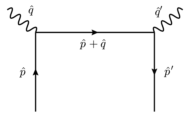
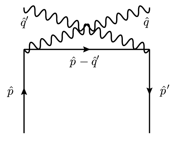
Figure 6: Two-quark leading order QCD diagrams.

To further illustrate the here-developed formalism and establish a connection with the traditional QCD approach, we present the calculation of the hard matching coefficients at leading order in $\alpha_{s}$.

5.1 Two-quark external states

We evaluate both sides of eq. (39) with a two-quark external states at $\alpha_{s}^{0}$ accuracy to obtain the coefficient functions $C_{\bar{\chi}\chi}^{[\Gamma]\mu\nu(0)}$ and $C_{\bar{\chi}\partial\chi}^{[\Gamma]\mu\nu\alpha(0)}$. Let

$$\hat{p}^{\mu} =(x+\eta)\bar{n}\cdot P\,\frac{n^{\mu}}{2}+P_{\perp}^{\mu},$$

$$\hat{p}^{\prime\mu} =(x-\eta)\bar{n}\cdot P\,\frac{n^{\mu}}{2}+P_{\perp}^{\mu},$$

$$\hat{q}^{\mu} =-(\rho+\eta)\bar{n}\cdot P\frac{n^{\mu}}{2}+\frac{Q^{2}}{\rho\bar{n}\cdot P}\frac{\bar{n}^{\mu}}{2},$$ (59)

$$\hat{q}^{\prime\mu} =-(\rho-\eta)\bar{n}\cdot P\frac{n^{\mu}}{2}+\frac{Q^{2}}{\rho\bar{n}\cdot P}\frac{\bar{n}^{\mu}}{2}.$$

We put the hats on the momenta to distinguish them from the physical momenta, but we will drop this notation for the rest of the section. It is implied that we are considering parton momenta.

The tree-level SCET matrix elements are

$$\bra{p^{\prime}}\mathcal{O}_{\bar{\chi}\chi}^{[\Gamma]}(-s/2,s/2)\ket{p}^{(0)} =e^{-is\bar{n}\cdot P}\bar{u}_{n}(p^{\prime})\frac{\Gamma}{2}u_{n}(p),$$

$$\bra{p^{\prime}}\mathcal{O}_{\bar{\chi}\partial\chi}^{[\Gamma]\alpha}(-s/2,s/2)\ket{p}^{(0)} =e^{-is\bar{n}\cdot P}\,P_{\perp}^{\alpha}\bar{u}_{n}(p^{\prime})\frac{\Gamma}{2}u_{n}(p),$$ (60)

where the superscript $(0)$ denotes the tree-level matrix elements. Thus

$$F_{\bar{\chi}\chi}^{[\Gamma](0)}(y) =\delta(x-y)\frac{\bar{u}_{n}(p^{\prime})\Gamma u_{n}(p)}{2\bar{n}\cdot P},$$

$$F_{\bar{\chi}\partial\chi}^{[\Gamma]\alpha(0)}(y) =\delta(x-y)\frac{P_{\perp}^{\alpha}}{\bar{n}\cdot P}\frac{\bar{u}_{n}(p^{\prime})\Gamma u_{n}(p)}{2\bar{n}\cdot P}.$$ (61)

Then, the right-hand side of eq. (39) reads

$$T_{qq}^{\mu\nu(0)} =\sum_{\Gamma\in\{\not{\bar{n}},\not{\bar{n}}\gamma_{5}\}}\Bigg{\{}C_{\bar{\chi}\chi}^{[\Gamma]\mu\nu(0)}(x)\frac{\bar{u}_{n}(p^{\prime})\Gamma u_{n}(p)}{2\bar{n}\cdot P}+C_{\bar{\chi}\partial\chi}^{[\Gamma]\mu\nu\alpha(0)}(x)\frac{P_{\perp\alpha}}{\bar{n}\cdot P}\frac{\bar{u}_{n}(p^{\prime})\Gamma u_{n}(p)}{2\bar{n}\cdot P}\Bigg{\}}.$$ (62)

The QCD contribution is given by the diagrams in figure 6:

$$T_{qq}^{\mu\nu(0)} =i\bar{u}(p^{\prime})\Bigg{\{}\gamma^{\nu}\frac{i}{\not{p}+\not{q}}\gamma^{\mu}+\gamma^{\mu}\frac{i}{\not{p}^{\prime}-\not{q}}\gamma^{\nu}\Bigg{\}}u(p)$$

$$=\frac{\bar{u}_{n}\not{\bar{n}}u_{n}}{\bar{n}\cdot P}\Bigg{\{}-g_{\perp}^{\mu\nu}\frac{x}{\rho^{2}-x^{2}}+\frac{P_{\perp\alpha}}{\bar{n}\cdot P}\Bigg{(}\frac{-(\eta\rho+x^{2})g_{\perp}^{\mu\alpha}\bar{n}^{\nu}+(\eta\rho-x^{2})g_{\perp}^{\nu\alpha}\bar{n}^{\mu}}{(\rho^{2}-x^{2})(\eta^{2}-x^{2})}$$

$$\qquad+\frac{(\bar{n}\cdot P)^{2}}{Q^{2}}\frac{\rho(\eta-\rho)(\eta\rho+x^{2})g_{\perp}^{\mu\alpha}n^{\nu}+\rho(\eta+\rho)(\eta\rho-x^{2})g_{\perp}^{\nu\alpha}n^{\mu}}{(\rho^{2}-x^{2})(\eta^{2}-x^{2})}\Bigg{)}\Bigg{\}}$$ (63)

$$\quad-i\frac{\bar{u}_{n}\not{\bar{n}}\gamma_{5}u_{n}}{\bar{n}\cdot P}\Bigg{\{}\varepsilon_{\perp}^{\mu\nu}\frac{\rho}{\rho^{2}-x^{2}}+\frac{P_{\perp\alpha}}{\bar{n}\cdot P}\Bigg{(}\frac{x(\eta-\rho)\varepsilon_{\perp}^{\nu\alpha}\bar{n}^{\mu}+x(\eta+\rho)\varepsilon_{\perp}^{\mu\alpha}\bar{n}^{\nu}}{(\rho^{2}-x^{2})(\eta^{2}-x^{2})}$$

$$\qquad+\frac{(\bar{n}\cdot P)^{2}}{Q^{2}}\frac{x\rho(\eta^{2}-\rho^{2})(\varepsilon_{\perp}^{\nu\alpha}n^{\mu}-\varepsilon_{\perp}^{\mu\alpha}n^{\nu})}{(\rho^{2}-x^{2})(\eta^{2}-x^{2})}\Bigg{)}\Bigg{\}}+\mathcal{O}(\lambda^{2}).$$

We now read off the coefficients functions:

$$C_{\bar{\chi}\chi}^{[\not{\bar{n}}]\mu\nu(0)}(x) =-2\frac{xg_{\perp}^{\mu\nu}}{\rho^{2}-x^{2}},$$

$$C_{\bar{\chi}\chi}^{[\not{\bar{n}}\gamma_{5}]\mu\nu(0)}(x) =-2i\frac{\rho\varepsilon_{\perp}^{\mu\nu}}{\rho^{2}-x^{2}},$$

$$C_{\bar{\chi}\partial\chi}^{[\not{\bar{n}}]\mu\nu\alpha(0)}(x) =-2\frac{(x^{2}+\eta\rho)g_{\perp}^{\mu\alpha}\bar{n}^{\nu}+(x^{2}-\eta\rho)g_{\perp}^{\nu\alpha}\bar{n}^{\mu}}{(\rho^{2}-x^{2})(\eta^{2}-x^{2})}$$ (64)

$$\qquad-2\kappa\frac{\rho(\rho-\eta)(x^{2}+\eta\rho)g_{\perp}^{\mu\alpha}n^{\nu}+\rho(\rho+\eta)(x^{2}-\eta\rho)g_{\perp}^{\nu\alpha}n^{\mu}}{(\rho^{2}-x^{2})(\eta^{2}-x^{2})},$$

$$C_{\bar{\chi}\partial\chi}^{[\not{\bar{n}}\gamma_{5}]\mu\nu\alpha(0)}(x) =-2i\frac{x(\rho+\eta)\varepsilon_{\perp}^{\mu\alpha}\bar{n}^{\nu}-x(\rho-\eta)\varepsilon_{\perp}^{\nu\alpha}\bar{n}^{\mu}}{(\rho^{2}-x^{2})(\eta^{2}-x^{2})}-2i\kappa\frac{x\rho(\rho^{2}-\eta^{2})(\varepsilon_{\perp}^{\mu\alpha}n^{\nu}-\varepsilon_{\perp}^{\nu\alpha}n^{\mu})}{(\rho^{2}-x^{2})(\eta^{2}-x^{2})},$$

where $\kappa=\frac{(\bar{n}\cdot P)^{2}}{Q^{2}}$.

We emphasize that in the SCET framework, the Feynman pole prescription $i0$ must be “inherited” by the on-shell QCD amplitude. Throughout this section, we have dropped the $i0$. To restore it, note that

$$(p+q)^{2}+i0 =-(\rho-x-\text{sgn}(Q^{2}/\rho)\,i0)Q^{2}/\rho,$$

$$(p-q^{\prime})^{2}+i0 =-(\rho+x-\text{sgn}(Q^{2}/\rho)\,i0)Q^{2}/\rho.$$ (65)

For DVCS, we have $\rho=\eta>0$ and $Q^{2}>0$ so that the pole prescription can be recovered by taking $\rho\rightarrow\rho-i0$. On the other hand, the $\frac{1}{\eta\pm x}$ denominators arose from eq. (20), so the prescription for this pole is a matter of choice, and the final result should not depend on it.

The DVCS coefficient functions are obtained by setting $\eta=\rho$ and $\nu=\perp$.

$$C_{\bar{\chi}\chi}^{[\not{\bar{n}}]\mu\nu(0)}(x) =-\frac{2xg_{\perp}^{\mu\nu}}{(\eta-x-i0)(\eta+x-i0)},$$

$$C_{\bar{\chi}\chi}^{[\not{\bar{n}}\gamma_{5}]\mu\nu(0)}(x) =-\frac{2\eta i\varepsilon_{\perp}^{\mu\nu}}{(\eta-x-i0)(\eta+x-i0)},$$

$$C_{\bar{\chi}\partial\chi}^{[\not{\bar{n}}]\mu\nu\alpha(0)}(x) =\frac{2g_{\perp}^{\nu\alpha}\bar{n}^{\mu}+4\kappa\eta^{2}g_{\perp}^{\nu\alpha}n^{\mu}}{(\eta-x-i0)(\eta+x-i0)},$$ (66)

$$C_{\bar{\chi}\partial\chi}^{[\not{\bar{n}}\gamma_{5}]\mu\nu\alpha(0)}(x) =0,$$

where we have explicitly included the $i0$ prescription. Interestingly, the $\sim\lambda^{1}$ axial-vector contribution vanishes. It is not clear whether this continues at higher orders. There are only simple poles at $x=\pm\eta$. Thus, if $F_{\bar{\chi}\partial\chi}^{[\not{\bar{n}}]\alpha}$ is continuous at $x\pm\eta$, the convolution integral is well-defined. It is well-known that certain twist-3 GPDs are in fact discontinuous at certain points. However, it is also well-known Kivel:2000cn that the convolution integrals are convergent nevertheless. We will see later, in section 6, that the coefficient functions in eq. (66) agree with the result from Kivel:2000cn .

5.2 Quark-gluon-quark external states

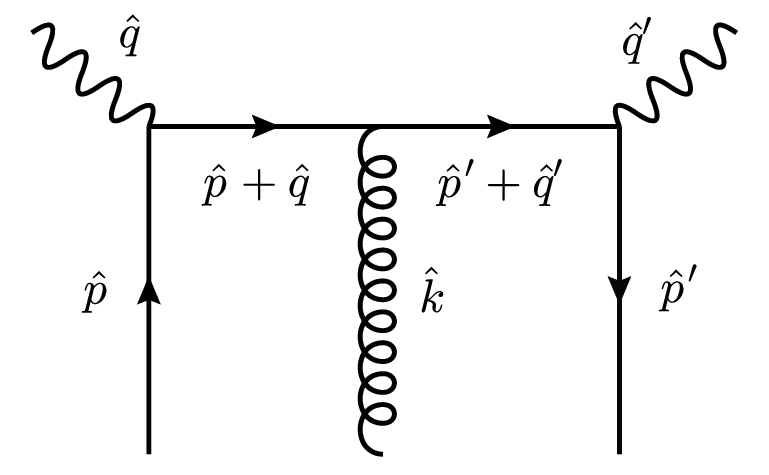
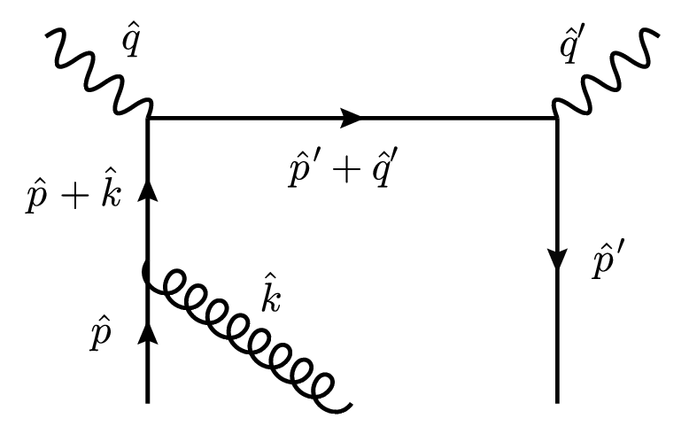
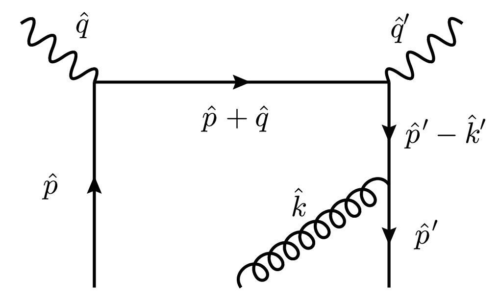
(a)                                       (b)                                      (c)

Figure 7: Quark-gluon-quark QCD diagrams. Diagrams with crossed photon legs also contribute but are not shown.

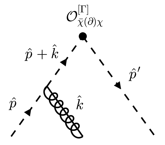
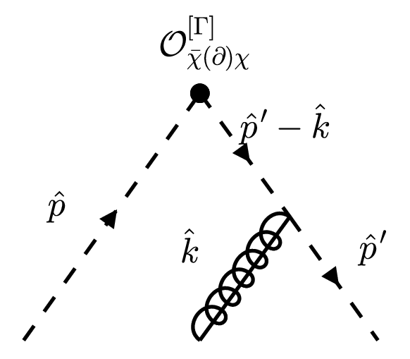
(a)                                   (b)

Figure 8: SCET diagrams contributing to the matching with quark-gluon-quark external states. At the top vertex we can have insertions of $\mathcal{O}_{\bar{\chi}\chi}^{[\Gamma]}$ or $\mathcal{O}_{\bar{\chi}\partial\chi}^{[\Gamma]\mu}$. Dashed propagators are $n$-collinear quarks, and the gluon propagator with lines through them denotes $n$-collinear gluons.

Let us choose external parton states with momenta

$$\hat{p}^{\mu} =(x_{1}-x_{2}+\eta)\bar{n}\cdot P\,\frac{n^{\mu}}{2}+P_{\perp}^{\mu}\,,$$

$$\hat{p}^{\prime\mu} =(x_{1}+x_{2}-\eta)\bar{n}\cdot P\,\frac{n^{\mu}}{2}+P_{\perp}^{\mu}\,,$$

$$\hat{k}^{\mu} =2x_{2}\bar{n}\cdot P\frac{n^{\mu}}{2}\,,$$ (67)

$$\hat{q}^{\mu} =-(\rho+\eta)\bar{n}\cdot P\frac{n^{\mu}}{2}+\frac{Q^{2}}{\rho\bar{n}\cdot P}\frac{\bar{n}^{\mu}}{2}\,,$$

$$\hat{q}^{\prime\mu} =-(\rho-\eta)\bar{n}\cdot P\frac{n^{\mu}}{2}+\frac{Q^{2}}{\rho\bar{n}\cdot P}\frac{\bar{n}^{\mu}}{2}\,.$$

Again, we drop the hats for the rest of this subsection, tacitly implying that we are considering partonic momenta. Here $\hat{k}$ is the ingoing momentum of the $n$-collinear gluon. The QCD diagrams are shown in figure 7. We have to keep $P_{\perp}$ for the quarks to regulate the $n$-collinear propagators of the diagrams (b) and (c) in figure 7. In the end, the limit $P_{\perp}^{\mu}\rightarrow 0$ should be taken since the additional gluon building block $\mathcal{A}_{n\perp}$ already presents a power of $\lambda$. The singularity as $P_{\perp}^{\mu}\rightarrow 0$ in the diagrams (b) and (c) in figure 7 will be canceled by the SCET diagrams with the insertion of the leading power operator $\mathcal{O}_{\bar{\chi}\chi}^{[\Gamma]}$ in figure 8. On the other hand, the insertion of $\mathcal{O}_{\bar{\chi}\partial\chi}^{[\Gamma]\alpha}$ will give a finite contribution (as $P_{\perp}^{\mu}\rightarrow 0$) to the matching. As for the polarization vector of the external gluon, we can choose it to be the unit-vector in $P_{\perp}$ direction, that is

$$\epsilon^{\mu}=-\frac{P_{\perp}^{\mu}}{\epsilon\cdot P_{\perp}}.$$ (68)

Let us start with the SCET part of the matching. We have

$$\bra{p^{\prime}}\mathcal{O}_{\bar{\chi}\mathcal{A}\chi}^{[\Gamma]\mu}(-s_{1}/2,s_{2}/2,s_{1}/2)\ket{p,k}^{(0)}=g\epsilon_{\perp}^{\mu}\bar{u}_{n}\frac{\Gamma}{2}u_{n}e^{-is_{1}x_{1}\bar{n}\cdot P-is_{2}x_{2}\bar{n}\cdot P}$$ (69)

and therefore

$$F_{\bar{\chi}\mathcal{A}\chi}^{[\Gamma]\mu(0)}(y_{1},y_{2})=g\epsilon_{\perp}^{\mu}\frac{\bar{u}_{n}\Gamma u_{n}}{2\bar{n}\cdot P}\delta(y_{1}-x_{1})\delta(y_{2}-x_{2}).$$ (70)

The contribution from the diagrams in figure 8 reads

$$\langle\mathcal{O}_{\bar{\chi}\chi}^{[\Gamma]}\rangle_{\text{fig}\,\ref{fig: qgq SCET dias}} =\bra{p^{\prime}}T\{\mathcal{O}_{\bar{\chi}\chi}^{[\Gamma]}(-s_{1}/2,s_{1}/2)$$

$$\quad\left[i\int d^{4}x\,\bar{\xi}\Big{(}g\not{A}_{n\perp}\frac{1}{i\bar{n}\cdot\partial}i\not{\partial}_{\perp}+i\not{\partial}_{\perp}\frac{1}{i\bar{n}\cdot\partial}g\not{A}_{n\perp}\Big{)}\frac{\not{\bar{n}}}{2}\xi\right]\}\ket{p,k}^{(0)}$$ (71)

$$=\frac{g\bar{u}_{n}\Gamma u_{n}}{2\epsilon\cdot P_{\perp}}\Bigg{\{}e^{-is_{1}(x_{1}+x_{2})\bar{n}\cdot P}\left(1+\frac{\bar{n}\cdot(p+k)}{\bar{n}\cdot p}\right)+e^{-is_{1}(x_{1}-x_{2})\bar{n}\cdot P}\left(1+\frac{\bar{n}\cdot(p^{\prime}-k)}{\bar{n}\cdot p^{\prime}}\right)\Bigg{\}}.$$

and

$$\langle\mathcal{O}_{\bar{\chi}\partial\chi}^{[\Gamma]\alpha}\rangle_{\text{fig}\,\ref{fig: qgq SCET dias}} =P_{\perp}^{\alpha}\langle\mathcal{O}_{\bar{\chi}\chi}^{[\Gamma]}\rangle_{\text{fig}\,\ref{fig: qgq SCET dias}}=-\epsilon\cdot P_{\perp}\epsilon^{\alpha}\langle\mathcal{O}_{\bar{\chi}\chi}^{[\Gamma]}\rangle_{\text{fig}\,\ref{fig: qgq SCET dias}}.$$ (72)

The contribution to the matching is obtained by convoluting with the coefficient functions:

$$(T_{qgq}^{\mu\nu})_{\text{fig}\,\ref{fig: qgq SCET dias}} =\sum_{\Gamma}\int_{-\infty}^{\infty}\frac{ds_{1}}{2\pi}\hat{C}_{\bar{\chi}\chi}^{[\Gamma]\mu\nu(0)}(s_{1})\langle\mathcal{O}_{\bar{\chi}\chi}^{[\Gamma]}\rangle_{\text{fig}\,\ref{fig: qgq SCET dias}}+\sum_{\Gamma}\int_{-\infty}^{\infty}\frac{ds_{1}}{2\pi}\hat{C}_{\bar{\chi}\partial\chi}^{[\Gamma]\mu\nu\alpha(0)}(s_{1})\langle\mathcal{O}_{\bar{\chi}\partial\chi\alpha}^{[\Gamma]}\rangle_{\text{fig}\,\ref{fig: qgq SCET dias}}$$

$$=\sum_{\Gamma}\frac{g\bar{u}_{n}\Gamma u_{n}}{2\bar{n}\cdot P}\frac{1}{\epsilon\cdot P_{\perp}}\Bigg{\{}C_{\bar{\chi}\chi}^{[\Gamma]\mu\nu(0)}(x_{1}+x_{2})\left(1+\frac{\bar{n}\cdot(p+k)}{\bar{n}\cdot p}\right)$$

$$\quad\quad+C_{\bar{\chi}\chi}^{[\Gamma]\mu\nu(0)}(x_{1}-x_{2})\left(1+\frac{\bar{n}\cdot(p^{\prime}-k)}{\bar{n}\cdot p^{\prime}}\right)\Bigg{\}}$$ (73)

$$\quad-\sum_{\Gamma}\frac{g\bar{u}_{n}\Gamma u_{n}}{2\bar{n}\cdot P}\epsilon_{\alpha}\Bigg{\{}C_{\bar{\chi}\partial\chi}^{[\Gamma]\mu\nu\alpha(0)}(x_{1}+x_{2})\left(1+\frac{\bar{n}\cdot(p+k)}{\bar{n}\cdot p}\right)$$

$$\quad\quad+C_{\bar{\chi}\partial\chi}^{[\Gamma]\mu\nu\alpha(0)}(x_{1}-x_{2})\left(1+\frac{\bar{n}\cdot(p^{\prime}-k)}{\bar{n}\cdot p^{\prime}}\right)\Bigg{\}}.$$

The contributions from the QCD diagrams are given by

$$(T_{qgq}^{\mu\nu})_{\text{fig}\,\ref{fig: qgq dias}(a)} =i\bar{u}_{n}\gamma^{\nu}\frac{i}{\not{p}^{\prime}+\not{q}^{\prime}}(ig\not{\epsilon}_{\perp})\frac{i}{\not{p}+\not{q}}\gamma^{\mu}u_{n}+i\bar{u}_{n}\gamma^{\mu}\frac{i}{\not{p}^{\prime}-\not{q}}(ig\not{\epsilon}_{\perp})\frac{i}{\not{p}-\not{q}^{\prime}}\gamma^{\nu}u_{n}$$ (74)

and

$$(T_{qgq}^{\mu\nu})_{{\rm fig}\,\ref{fig: qgq dias}(b)+(c)} =g\bar{u}(p^{\prime})\Bigg{\{}\not{\epsilon}_{\perp}\frac{1}{\not{p}^{\prime}-\not{k}}\left(\gamma^{\nu}\frac{1}{\not{p}+\not{q}}\gamma^{\mu}+\gamma^{\mu}\frac{1}{\not{p}-\not{q}^{\prime}}\gamma^{\nu}\right)$$

$$\quad+\left(\gamma^{\nu}\frac{1}{\not{p}^{\prime}+\not{q}^{\prime}}\gamma^{\mu}+\gamma^{\mu}\frac{1}{\not{p}^{\prime}-\not{q}}\gamma^{\nu}\right)\frac{1}{\not{p}+\not{k}}\not{\epsilon}_{\perp}\Bigg{\}}u(p).$$ (75)

To summarize, the matching equation reads

$$\sum_{\Gamma}g\epsilon_{\perp\alpha}\frac{\bar{u}_{n}\Gamma u_{n}}{2\bar{n}\cdot P}C_{\bar{\chi}\mathcal{A}\chi}^{[\Gamma]\mu\nu\alpha}(x_{1},x_{2})=(T_{qgq}^{\mu\nu})_{\text{fig}\,\ref{fig: qgq dias}}-(T_{qgq}^{\mu\nu})_{\text{fig}\,\ref{fig: qgq SCET dias}}.$$ (76)

A straightforward calculation gives

$$C_{\bar{\chi}A\chi}^{[\not{\bar{n}}]\mu\nu\alpha(0)} =2\bar{n}^{\mu}g_{\perp}^{\nu\alpha}\frac{x_{1}^{2}-\left(\eta+x_{2}\right)\left(\rho-x_{2}\right)}{\left(-\eta+x_{1}-x_{2}\right)\left(\eta+x_{1}+x_{2}\right)\left(\rho-x_{1}-x_{2}\right)\left(\rho+x_{1}-x_{2}\right)}$$

$$\quad+2n^{\mu}g_{\perp}^{\nu\alpha}\frac{\kappa\rho(\eta+\rho)\left(x_{1}^{2}-\left(\eta+x_{2}\right)\left(\rho-x_{2}\right)\right)}{\left(-\eta+x_{1}-x_{2}\right)\left(\eta+x_{1}+x_{2}\right)\left(\rho-x_{1}-x_{2}\right)\left(\rho+x_{1}-x_{2}\right)}$$ (77)

$$\quad+(\mu\leftrightarrow\nu,\rho\rightarrow-\rho),$$

$$C_{\bar{\chi}A\chi}^{[\not{\bar{n}}\gamma_{5}]\mu\nu\alpha(0)} =2\bar{n}^{\mu}i\varepsilon_{\perp}^{\nu\alpha}\frac{x_{1}\left(\eta-\rho+2x_{2}\right)}{\left(\eta-x_{1}+x_{2}\right)\left(\eta+x_{1}+x_{2}\right)\left(\rho+x_{1}-x_{2}\right)\left(-\rho+x_{1}+x_{2}\right)}$$

$$\quad+2n^{\mu}i\varepsilon_{\perp}^{\nu\alpha}\frac{\kappa\rho x_{1}(\eta+\rho)\left(\eta-\rho+2x_{2}\right)}{\left(-\eta+x_{1}-x_{2}\right)\left(\eta+x_{1}+x_{2}\right)\left(\rho-x_{1}-x_{2}\right)\left(\rho+x_{1}-x_{2}\right)}$$ (78)

$$\quad+(\mu\leftrightarrow\nu,\rho\rightarrow-\rho).$$

Interestingly, we have

$$C_{\bar{\chi}\partial\chi}^{[\Gamma]\mu\nu\alpha(0)}(x)=C_{\bar{\chi}\mathcal{A}\chi}^{[\Gamma]\mu\nu\alpha(0)}(x,0).$$ (79)

This implies that, at the tree level, the complete NLP contribution, apart from pure gluon contributions, can be written as

$$T_{\rm NLP}^{\mu\nu(0)} =\sum_{\Gamma}\int_{-\infty}^{\infty}\frac{ds_{1}ds_{2}}{(2\pi)^{2}}\,\hat{C}_{\bar{\chi}\mathcal{A}\chi}^{[\Gamma]\mu\nu\alpha}(s_{1},s_{2})$$

$$\quad\times\bra{p^{\prime}}\bar{\chi}_{n}(-s_{1}\bar{n}/2)\Big{(}i\overleftrightarrow{\partial}_{\perp}^{\mu}+\mathcal{A}_{n\perp}(s_{2}\bar{n}/2)\Big{)}\frac{\Gamma}{2}\chi(s_{1}\bar{n}/2)\ket{p},$$ (80)

where $\Gamma\in\{\not{\bar{n}},\not{\bar{n}}\gamma_{5}\}$ and

$$\hat{C}_{\bar{\chi}\mathcal{A}\chi}^{[\Gamma]\mu\nu\alpha}(s_{1},s_{2})=\int_{-\infty}^{\infty}dx_{1}dx_{2}\,e^{ix_{1}s_{1}\bar{n}\cdot P+ix_{2}s_{2}\bar{n}\cdot P}C_{\bar{\chi}\mathcal{A}\chi}^{[\Gamma]\mu\nu\alpha}(x_{1},x_{2}).$$ (81)

As it stands, there is no compelling reason to believe that this continues beyond tree level.

6 Connection with the traditional approach

In this section, we use light-cone $\bar{n}\cdot A=0$ gauge for simplicity, though working in a general gauge, while being more tedious, is a straightforward generalization. In the traditional approach, one calculates the diagrams in figure 6 and 7(a) in terms of the QCD correlators

$$F^{\mu}(x) =\int_{-\infty}^{\infty}\frac{ds}{2\pi}e^{ixs\bar{n}\cdot P}\bra{p^{\prime}}\bar{\psi}(-s\bar{n}/2)\frac{\gamma^{\mu}}{2}\psi(s\bar{n}/2)\ket{p},$$

$$\widetilde{F}^{\mu}(x) =\int_{-\infty}^{\infty}\frac{ds}{2\pi}e^{ixs\bar{n}\cdot P}\bra{p^{\prime}}\bar{\psi}(-s\bar{n}/2)\frac{\gamma^{\mu}}{2}\gamma_{5}\psi(s\bar{n}/2)\ket{p},$$

$$K_{\perp}^{\mu}(x) =\frac{1}{\bar{n}\cdot P}\int_{-\infty}^{\infty}\frac{ds}{2\pi}e^{ixs\bar{n}\cdot P}\bra{p^{\prime}}\bar{\psi}(-s\bar{n}/2)i\overleftrightarrow{\partial}_{\perp}^{\mu}\frac{\not{\bar{n}}}{2}\psi(s\bar{n}/2)\ket{p},$$

$$\widetilde{K}_{\perp}^{\mu}(x) =\frac{1}{\bar{n}\cdot P}\int_{-\infty}^{\infty}\frac{ds}{2\pi}e^{ixs\bar{n}\cdot P}\bra{p^{\prime}}\bar{\psi}(-s\bar{n}/2)i\overleftrightarrow{\partial}_{\perp}^{\mu}\frac{\not{\bar{n}}}{2}\gamma_{5}\psi(s\bar{n}/2)\ket{p},$$ (82)

$$S_{\perp}^{\mu}(x_{1},x_{2}) =\int_{-\infty}^{\infty}\frac{ds_{1}}{2\pi}\frac{ds_{2}}{2\pi}e^{is_{1}x_{1}\bar{n}\cdot P+is_{2}x_{2}\bar{n}\cdot P}\bra{p^{\prime}}\bar{\psi}(-s_{1}\bar{n}/2)gA_{\perp}^{\mu}(s_{2}\bar{n}/2)\frac{\not{\bar{n}}}{2}\psi(s_{1}\bar{n}/2)\ket{p},$$

$$\widetilde{S}_{\perp}^{\mu}(x_{1},x_{2}) =\int_{-\infty}^{\infty}\frac{ds_{1}}{2\pi}\frac{ds_{2}}{2\pi}e^{is_{1}x_{1}\bar{n}\cdot P+is_{2}x_{2}\bar{n}\cdot P}\bra{p^{\prime}}\bar{\psi}(-s_{1}\bar{n}/2)gA_{\perp}^{\mu}(s_{2}\bar{n}/2)\frac{\not{\bar{n}}}{2}\gamma_{5}\psi(s_{1}\bar{n}/2)\ket{p}.$$

In a general gauge, the definitions need to be modified by inserting Wilson lines, which ensure gauge invariance.

Note that the diagrams in figure 7 (b) and (c) are explicitly not included in the standard approach since they are one-particle reducible in the external parton legs and, therefore, do not contribute to the hard scattering amplitude. This seemingly breaks the electromagnetic Ward identity since we do not sum up all possible insertions of the photons. However, the missing terms are in some sense “hidden” in the $F_{\perp}^{\mu}$ and $\widetilde{F}_{\perp}^{\mu}$ components Belitsky:2005qn . The electromagnetic gauge invariance is restored after eliminating them using the equations of motion. In SCET, this step is performed at the Lagrangian level by integrating out the subleading spinor components of the quark field, which amounts to solving the equations of motion for those components so that it presents a more systematic approach to factorizing the amplitude at NLP.

To obtain the known result from the ${\rm SCET}$ result, note that a pure collinear SCET Lagrangian after ultrasoft decoupling transformation is equivalent to the QCD Lagrangian. Therefore, the correlators in eq. (82) correspond to the functions $F_{\ell}$ introduced in section 4, upon replacing $\psi\leftrightarrow\xi_{n}$ and $A^{\mu}\leftrightarrow A_{n}^{\mu}$.

However, this identification is not straightforward since it depends on how the GPD in QCD is defined. Do the correlators in (82) include ultrasoft modes? In what sense should one understand the GPD near $x=\pm\eta$, i.e., when the partons are not $n$-collinear? Note that since ultrasoft and $n$-collinear modes can only interact by subleading power Lagrangians (up to scalar-polarized gluons), this distinction is usually only relevant beyond leading power. This work will not attempt to answer these questions or state the “correct” definition of GPD. The ambiguity is entirely characterized by the contribution in eq. (55). Up to this subtlety, the identification $\psi\leftrightarrow\xi_{n}$ and $A^{\mu}\leftrightarrow A_{n}^{\mu}$ should be valid at NLP accuracy, but not beyond.

Another (somewhat less subtle) complication is given by the transverse components $F_{\perp}^{\mu}$. In ${\rm SCET}$ one has integrated out the subleading spinor components so that $\bar{\xi}_{n}\gamma_{\perp}^{\mu}\xi_{n}=0$. However, the pure collinear Lagrangian is equivalent to a copy of the QCD Lagrangian. We can formally reintroduce the subleading spinor components and obtain direct correspondence. Since an $\not{\bar{n}}$ between parton fields projects them onto the leading spinor components anyway, we can identify

$$\bar{n}\cdot F\longleftrightarrow F_{\bar{\chi}\chi}^{[\not{\bar{n}}]},\qquad\bar{n}\cdot\widetilde{F}\longleftrightarrow F_{\bar{\chi}\chi}^{[\not{\bar{n}}\gamma_{5}]},$$

$$K_{\perp}^{\mu}\longleftrightarrow F_{\bar{\chi}\partial\chi}^{[\not{\bar{n}}]\mu},\qquad\widetilde{K}_{\perp}^{\mu}\longleftrightarrow F_{\bar{\chi}\partial\chi}^{[\not{\bar{n}}\gamma_{5}]\mu},$$ (83)

$$S_{\perp}^{\mu}\longleftrightarrow F_{\bar{\chi}\mathcal{A}\chi}^{[\not{\bar{n}}]\mu},\qquad\widetilde{S}_{\perp}^{\mu}\longleftrightarrow F_{\bar{\chi}\mathcal{A}\chi}^{[\not{\bar{n}}\gamma_{5}]\mu}.$$

The functions $F_{\perp}^{\mu}$ and $\widetilde{F}_{\perp}^{\mu}$ are related to $K_{\perp}^{\mu},\widetilde{K}_{\perp}^{\mu},S_{\perp}^{\mu},\widetilde{S}_{\perp}^{\mu}$ by the QCD equations of motion. In fact, one can readily show that

$$K_{\perp}^{\mu}(x)-xF_{\perp}^{\mu}(x)+i\varepsilon_{\perp}^{\mu\nu}\eta\widetilde{F}_{\perp\nu}(x)$$

$$=-\frac{1}{2}\int_{-\infty}^{\infty}dx_{1}dx_{2}\Bigg{\{}\Big{[}\delta(x-x_{1}+x_{2})+\delta(x-x_{1}-x_{2})\Big{]}S_{\perp}^{\mu}(x_{1},x_{2})$$ (84)

$$\quad+\Big{[}\delta(x-x_{1}+x_{2})-\delta(x-x_{1}-x_{2})\Big{]}i\varepsilon_{\perp}^{\mu\nu}\widetilde{S}_{\perp\nu}(x_{1},x_{2})\Bigg{\}}$$

and

$$\widetilde{K}_{\perp}^{\mu}(x)-x\widetilde{F}_{\perp}^{\mu}(x)+i\varepsilon_{\perp}^{\mu\nu}\eta F_{\perp\nu}(x)$$

$$=-\frac{1}{2}\int_{-\infty}^{\infty}dx_{1}dx_{2}\Bigg{\{}\Big{[}\delta(x-x_{1}+x_{2})+\delta(x-x_{1}-x_{2})\Big{]}\widetilde{S}_{\perp}^{\mu}(x_{1},x_{2})$$ (85)

$$\quad+\Big{[}\delta(x-x_{1}+x_{2})-\delta(x-x_{1}-x_{2})\Big{]}i\varepsilon_{\perp}^{\mu\nu}S_{\perp\nu}(x_{1},x_{2})\Bigg{\}}.$$

To obtain the standard result we can eliminate $K_{\perp}^{\mu}$ and $\widetilde{K}_{\perp}^{\mu}$, by the virtue of eqs. (84) and (85), in the factorization formula eq. (39). Hence

$$T^{\mu\nu(0)} =\int_{-\infty}^{\infty}dx\,\Big{\{}C_{\bar{\chi}\chi}^{[\not{\bar{n}}]\mu\nu(0)}\bar{n}\cdot F+C_{\bar{\chi}\chi}^{[\not{\bar{n}}\gamma_{5}]\mu\nu(0)}\bar{n}\cdot\widetilde{F}+C_{\bar{\chi}\partial\chi}^{[\not{\bar{n}}]\mu\nu\alpha(0)}K_{\perp\alpha}+C_{\bar{\chi}\partial\chi}^{[\not{\bar{n}}\gamma_{5}]\mu\nu\alpha(0)}\widetilde{K}_{\perp\alpha}$$

$$\quad+C_{\bar{\chi}\mathcal{A}\chi}^{[\not{\bar{n}}]\mu\nu\alpha(0)}S_{\perp\alpha}+C_{\bar{\chi}\mathcal{A}\chi}^{[\not{\bar{n}}\gamma_{5}]\mu\nu\alpha(0)}\widetilde{S}_{\perp\alpha}\Big{\}}$$

$$=\int_{-\infty}^{\infty}dx\,C_{-}\Big{\{}-g_{\perp}^{\mu\nu}\bar{n}\cdot F+F_{\perp}^{\mu}(\bar{n}^{\nu}+\rho(\rho-\eta)\kappa n^{\nu})+F_{\perp}^{\nu}(\bar{n}^{\mu}+\rho(\rho+\eta)\kappa n^{\mu})\Big{\}}$$ (86)

$$\quad+\int_{-\infty}^{\infty}dx\,C_{+}\Big{\{}-i\varepsilon_{\perp}^{\mu\nu}\bar{n}\cdot\widetilde{F}+i\varepsilon_{\perp}^{\mu\alpha}\widetilde{F}_{\alpha}(\bar{n}^{\nu}+\kappa\rho(\rho-\eta)n^{\nu})-i\varepsilon_{\perp}^{\nu\alpha}\widetilde{F}_{\alpha}(\bar{n}^{\mu}+\kappa\rho(\rho+\eta)n^{\mu})\Big{\}},$$

where

$$C_{\pm}(x)=\frac{1}{\rho-x}\pm\frac{1}{\rho+x}.$$ (87)

Eq. (86) agrees with the known results in Kivel:2000cn , considering that we are working the BMJ frame, where $\Delta_{\perp}=0$. The results for the other frames can readily be recovered by redefining the light-cone vectors, which is discussed in the following section 7.

Interestingly, the quark-gluon-quark contribution cancels entirely at the tree level. Of course, this observation is far from new, see e.g. Anikin:2000em ; Penttinen:2000dg ; Belitsky:2000vx ; Radyushkin:2000jy . It is equivalent to the statement in eq. (80). As mentioned, we do not see why this should continue at higher orders.

7 RPI and transformation to other frames

Throughout this section, we shall drop terms of $\mathcal{O}(\lambda^{2})$. The central statement of reparametrization invariance is that observables – in this case, we apply this to the hadronic tensor $T^{\mu\nu}$ – are invariant under certain redefinitions of the light-cone vectors $n$ and $\bar{n}$, that preserve the scaling of the external momenta. See, for example, Marcantonini:2008qn for a characterization of such transformations.

A general RPI transformation takes one from $(n,\bar{n})$ light-cone basis to another light-cone system $(w,\bar{w})$. A generic vector $v^{\mu}$ can then be written in both coordinates as

$$v^{\mu}=n\cdot v\frac{\bar{n}^{\mu}}{2}+\bar{n}\cdot v\frac{n^{\mu}}{2}+v_{\perp}^{\mu}=w\cdot v\frac{\bar{w}^{\mu}}{2}+\bar{w}\cdot v\frac{w^{\mu}}{2}+v^{\perp\mu}.$$ (88)

Naturally, we demand $w^{2}=\bar{w}^{2}=w\cdot\bar{w}-2=0,\,w\cdot v^{\perp}=\bar{w}\cdot v^{\perp}=0$. Furthermore, we define

$$g^{\perp\mu\nu}=g^{\mu\nu}-\frac{1}{2}w^{\mu}\bar{w}^{\nu}-\frac{1}{2}w^{\nu}\bar{w}^{\mu},\qquad\varepsilon^{\perp\mu\nu}=\varepsilon^{\mu\nu\alpha\beta}\frac{1}{2}w_{\alpha}\bar{w}_{\beta}.$$ (89)

We start by converting our result from the BMP to the KP frame. The transformation that takes one from the BMP $(n,\bar{n})$ frame to the KP $(w,\bar{w})$ frame is given by

$$n^{\mu}=w^{\mu}+\delta_{1}^{\mu},\qquad\bar{n}^{\mu}=\bar{w}^{\mu}+\delta_{2}^{\mu},\qquad$$

$$v^{\perp\mu}=v_{\perp}^{\mu}+\delta_{1}\cdot v\,\frac{\bar{n}^{\mu}}{2}+\delta_{2}\cdot v\frac{n^{\mu}}{2}+\bar{n}\cdot v\frac{\delta_{1}^{\mu}}{2}+n\cdot v\frac{\delta_{2}^{\mu}}{2},$$ (90)

where

$$\delta_{1}^{\mu}=\frac{2\Delta^{\perp\mu}}{\bar{n}\cdot\Delta}=-\frac{2P_{\perp}^{\mu}}{\bar{n}\cdot P},\qquad\delta_{2}^{\mu}=-\frac{2\Delta^{\perp\mu}\bar{n}\cdot q}{\bar{n}\cdot\Delta\,n\cdot q^{\prime}}.$$ (91)

Since $\delta_{1}\sim\delta_{2}\sim\lambda$, this does not change the scaling of external momenta and is an allowed RPI transformation. One can easily compute

$$g_{\perp}^{\mu\nu} =g^{\perp\mu\nu}+\frac{1}{2\eta\bar{n}\cdot P}(\Delta^{\perp\mu}\bar{w}^{\nu}+\Delta^{\perp\nu}\bar{w}^{\mu})+\frac{\rho(\rho+\eta)}{2\eta\bar{n}\cdot P}\frac{(\bar{n}\cdot P)^{2}}{Q^{2}}(w^{\mu}\Delta^{\perp\nu}+w^{\nu}\Delta^{\perp\mu}),$$ (92)

$$\varepsilon_{\perp}^{\mu\nu} =\varepsilon^{\perp\mu\nu}-\frac{\bar{w}^{\mu}\varepsilon^{\perp\nu\alpha}\Delta^{\perp}_{\alpha}}{2\eta\bar{n}\cdot P}+\frac{\bar{w}^{\nu}\varepsilon^{\perp\mu\alpha}\Delta^{\perp}_{\alpha}}{2\eta\bar{n}\cdot P}$$

$$\quad-\rho(\rho+\eta)\frac{(\bar{n}\cdot P)^{2}}{Q^{2}}\frac{w^{\mu}\varepsilon^{\perp\nu\alpha}\Delta^{\perp}_{\alpha}}{2\eta\bar{n}\cdot P}+\rho(\rho+\eta)\frac{(\bar{n}\cdot P)^{2}}{Q^{2}}\frac{w^{\nu}\varepsilon^{\perp\mu\alpha}\Delta^{\perp}_{\alpha}}{2\eta\bar{n}\cdot P}.$$ (93)

The only operator that transforms at $\lambda^{1}$ accuracy is $\mathcal{O}_{\bar{\chi}\partial\chi}^{[\Gamma]}$. Indeed, we have

$$\bar{\chi}(-s\bar{n}/2)\frac{\Gamma}{2}i\overleftrightarrow{\partial}_{\perp}^{\mu}\chi(s\bar{n}/2) =\bar{\chi}(-s\bar{n}/2)\frac{\Gamma}{2}i\overleftrightarrow{\partial}^{\perp\mu}\chi(s\bar{n}/2)-i\frac{\Delta^{\perp\mu}}{\bar{n}\cdot\Delta}\frac{d}{ds}\bar{\chi}(-s\bar{n}/2)\frac{\Gamma}{2}\chi(s\bar{n}/2).$$ (94)

Taking matrix elements and Fourier transforming gives the

$$F_{\bar{\chi}\partial\chi\perp}^{[\Gamma]\mu}=F_{\bar{\chi}\partial\chi}^{[\Gamma]\perp\mu}-\frac{x\Delta^{\perp\mu}}{\bar{n}\cdot\Delta}F_{\bar{\chi}\chi}^{[\Gamma]}.$$ (95)

To compare with the result from Kivel:2000cn , we also need to consider the term proportional to $\Delta^{\perp}$ from the equations of motion relation that were dropped in eqs. (84) and (85). Ignoring the quark-gluon-quark contributions, since they cancel anyways, we have

$$K^{\perp\mu} =xF^{\perp\mu}-i\varepsilon^{\perp\mu\nu}\eta\widetilde{F}^{\perp}_{\nu}-\frac{i}{2}\varepsilon^{\perp\mu\nu}\frac{\Delta^{\perp}_{\nu}}{\bar{n}\cdot P}\bar{n}\cdot\widetilde{F},$$ (96)

$$\widetilde{K}^{\perp\mu} =x\widetilde{F}^{\perp\mu}-i\varepsilon^{\perp\mu\nu}\eta F^{\perp}_{\nu}-\frac{i}{2}\varepsilon^{\perp\mu\nu}\frac{\Delta^{\perp}_{\nu}}{\bar{n}\cdot P}\bar{n}\cdot F.$$ (97)

Taking into account all these contributions, we find that the shift $\delta T=T-T|_{(n,\bar{n})\rightarrow(w,\bar{w})}$ due to changing the coordinates is

$$\delta T^{\mu\nu(0)}=-\int_{-\infty}^{\infty}dx\,\Big{(}g^{\perp\mu\alpha}C_{-}\bar{n}\cdot F+i\varepsilon^{\perp\mu\alpha}C_{+}\bar{n}\cdot\widetilde{F}\Big{)}\frac{\Delta^{\perp}_{\alpha}P^{\nu}}{P\cdot q},$$ (98)

in agreement with Kivel:2000cn .

For completeness, we also give the results for the RPI transformation to the Compton frame. It has the same form as in eq. (90) with

$$\delta_{1}^{\mu}=\frac{2\Delta^{\perp\mu}}{\bar{n}\cdot\Delta},\qquad\delta_{2}^{\mu}=-\frac{2\Delta^{\perp\mu}\,\bar{n}\cdot(q+q^{\prime})}{\bar{n}\cdot\Delta\,n\cdot(q+q^{\prime})}.$$ (99)

The result is

$$\delta T^{\mu\nu(0)}=-\int_{-\infty}^{\infty}dx\,\Delta^{\perp}_{\alpha}\Bigg{\{}C_{-}\bar{n}\cdot F\Big{(}\frac{g^{\perp\mu\alpha}P^{\nu}-g^{\perp\nu\alpha}P^{\mu}}{2P\cdot q}\Big{)}+C_{+}\bar{n}\cdot\widetilde{F}\Big{(}\frac{i\epsilon^{\perp\mu\alpha}P^{\nu}+i\epsilon^{\perp\nu\alpha}P^{\mu}}{2P\cdot q}\Big{)}\Bigg{\}},$$ (100)

in agreement with Belitsky:2005qn .

8 Conclusions and Outlook

We have given an in-depth analysis of the factorization of DVCS at NLP using SCET. We conclude that, at least for DDVCS, where both photons are far off-shell, the amplitude factorizes to all orders in terms of twist-3 GPDs in exactly the form that was hypothesized in the literature, as given in eq. (39). The corresponding SCET operators were given in eqs. (31) and (32). In section 5, we performed the corresponding tree-level matching in the SCET formalism, and in section 6, we compared and found agreement of the coefficient functions with the known results in the literature. In section 7, the RPI has been used to convert the results into various frames.

The most interesting issue appears when one photon is on-shell, as in DVCS. In section 4, we identified an endpoint-like contribution of parametrical size $\Lambda_{\rm QCD}/Q$, which does factorize but presents a possible problem for the universality (or process-independence) of the GPD description of DVCS at NLP. We have given a precise all-order formula for this contribution in eq. (55), which should be added to the result in eq. (39). The contribution in (55) involves ultrasoft and $\bar{n}$-collinear regions, corresponding to the region where a parton becomes ultrasoft. This region “overlaps” with the endpoint-like regions of the convolution integral where $x\pm\eta\sim\lambda^{2}$. It should not be confused with the Glauber region (which is absent, i.e., not pinched, in DVCS at this accuracy) that also overlaps with the endpoint-like regions and has been observed to break factorization in other processes involving GPDs Braun:2002wu ; Nabeebaccus:2023rzr . We stress that in DVCS, there is no endpoint-like divergence due to the contribution in (55), at least up to NLO Kivel:2003jt . Moreover, it vanishes perturbatively for massless quarks due to chiral symmetry, but it is non-zero non-perturbatively due to the spontaneous symmetry breaking of chiral symmetry in QCD. It remains unclear whether this contribution is phenomenologically relevant or, in other words, whether the contribution of eq. (55) is actually of a similar size as the contribution of eq. (39). A numerical study investigating this involves an at least somewhat realistic estimate for the non-perturbative (ultrasoft $\mathcal{I}_{s}$ and $n$-collinear $\mathcal{I}_{n}$) contributions in eq. (55), which is beyond the scope of this work.

Although there are many open questions regarding factorization revolving around processes involving GPDs, what SCET can bring to this field of study, particularly beyond the leading power, has not been investigated. This work provides a first step in this direction by applying the framework of the most prominent GPD process, DVCS. A natural example of another process where these methods might be useful, is deeply virtual meson production for transverse virtual photon polarizations (at leading power). The reduced graph gives the leading region in figure 5(b) with the external photon being exchanged with a light meson Collins:1996fb . A contribution analogous to eq. (55) describes this region. In particular, the same non-perturbative factor appears; therefore, at least for these two processes, the non-perturbative part of eq. (55) is actually “universal”.

Moreover, SCET provides a systematic approach to the power expansion, which can be straightforwardly generalized beyond the leading order in $\alpha_{s}$. Going to the next-to-leading order will not only be conceptually interesting, but it will also be relevant for DVCS phenomenology. At this accuracy, one can expect that the genuine twist-3 operators enter, particularly the pure gluon operators in eq. (32).

Appendix A SCET Lagrangian at next-to-leading power

The ${\rm SCET_{I}}$ Lagrangian at $\mathcal{O}(\lambda^{1})$ accuracy in position space formalism Beneke:2002ni reads

$$\mathcal{L}_{\rm SCET_{I}} =\mathcal{L}_{n}^{(0)}(\xi_{n},A_{n},A_{s})+\mathcal{L}_{\bar{n}}^{(0)}(\xi_{\bar{n}},A_{\bar{n}},A_{s})+\mathcal{L}_{s}^{(0)}(q_{s},A_{s})$$

$$\quad+\mathcal{L}_{ns}^{(1)}(\xi_{n},q_{s},A_{n},A_{s})+\mathcal{L}_{\bar{n}s}^{(1)}(\xi_{\bar{n}},q_{s},A_{\bar{n}},A_{s})+\mathcal{O}(\lambda^{2}/d^{4}x),$$ (101)

where

$$\frac{\lambda^{0}}{d^{4}x}\sim\mathcal{L}_{n}^{(0)} =\bar{\xi}_{n}\Big{(}in\cdot D_{n}+gn\cdot A_{s}+i\not{D}_{n\perp}\frac{1}{i\bar{n}\cdot D_{n}}i\not{D}_{n\perp}\Big{)}\frac{\not{\bar{n}}}{2}\xi_{n}-\frac{1}{2}\text{tr}(F_{n}^{\mu\nu}F_{n\mu\nu})$$

$$\frac{\lambda^{0}}{d^{4}x}\sim\mathcal{L}_{s}^{(0)} =\bar{q}_{s}i\not{D}_{s}q_{s}-\frac{1}{2}\text{tr}(F_{s}^{\mu\nu}F_{s\mu\nu})$$

$$\frac{\lambda^{1}}{d^{4}x}\sim\mathcal{L}_{ns}^{(1)} =\bar{\xi}_{n}x_{\perp}^{\mu}n^{\nu}W_{n}gF_{s,\mu\nu}^{[n]}W_{n}^{\dagger}\frac{\not{\bar{n}}}{2}\xi_{n}+\bar{q}_{s}^{[n]}W_{n}^{\dagger}i\not{D}_{n\perp}\xi_{n}-\bar{\xi}_{n}i\overleftarrow{\not{D}}_{n\perp}W_{n}q_{s}^{[n]}$$ (102)

$$\quad+\text{tr}\Big{(}\bar{n}^{\mu}F_{n\mu j}W_{n}i\Big{[}x_{\perp}^{\rho}n^{\sigma}F_{s\rho\sigma}^{[n]},W_{n}^{\dagger}(iD_{n}^{j}W_{n})\Big{]}W_{n}^{\dagger}\Big{)}-\text{tr}\Big{(}\bar{n}_{\mu}F_{n}^{\mu j}W_{n}n^{\rho}F_{s\rho j}^{[n]}W_{n}^{\dagger}\Big{)}.$$

The Lagrangians $\mathcal{L}_{\bar{n}}^{(0)}$ and $\mathcal{L}_{\bar{n}s}^{(1)}$ are the same with $n\leftrightarrow\bar{n}$. In the following, the corresponding definitions with $n\leftrightarrow\bar{n}$ can be obtained by this replacement.

A superscript $[n]$ means that the soft fields are multipole expanded with respect to the $n$-collinear direction

$$f^{[n]}(x)=f\Big{(}\bar{n}\cdot x\frac{n}{2}\Big{)}.$$ (103)

The covariant derivatives are defined as

$$D_{n}^{\mu}=\partial^{\mu}-igA_{n}^{\mu},\qquad D_{s}^{\mu}=\partial^{\mu}-igA_{s}^{\mu}.$$ (104)

The collinear and soft Wilson lines are defined by

$$W_{n} =P\exp\Big{(}ig\int_{-\infty}^{0}ds\,\bar{n}\cdot A_{n}(x+s\bar{n})\Big{)},$$ (105)

$$Y_{n} =P\exp\Big{(}ig\int_{-\infty}^{0}ds\,n\cdot A_{s}(x+sn)\Big{)}.$$ (106)

The ultrasoft field strength tensor is just the usual field strength tensor expressed in terms of corresponding ultrasoft covariant derivative

$$F_{s}^{\mu\nu}=\frac{i}{g}[D_{s}^{\mu},D_{s}^{\nu}]$$ (107)

and the collinear field strength tensor is defined as

$$F_{n}^{\mu\nu}=\frac{i}{g}\left[D_{n}^{\mu}-ig\frac{\bar{n}^{\mu}}{2}n\cdot A_{s},D_{n}^{\nu}-ig\frac{\bar{n}^{\nu}}{2}n\cdot A_{s}\right].$$ (108)

References

- (1) D. Müller, D. Robaschik, B. Geyer, F.M. Dittes and J. Hořejši, Wave functions, evolution equations and evolution kernels from light ray operators of QCD, Fortsch. Phys. 42 (1994) 101 [hep-ph/9812448].
- (2) X.-D. Ji, Gauge-Invariant Decomposition of Nucleon Spin, Phys. Rev. Lett. 78 (1997) 610 [hep-ph/9603249].
- (3) X.-D. Ji, Deeply virtual Compton scattering, Phys. Rev. D 55 (1997) 7114 [hep-ph/9609381].
- (4) A.V. Radyushkin, Nonforward parton distributions, Phys. Rev. D 56 (1997) 5524 [hep-ph/9704207].
- (5) M. Burkardt, Impact parameter space interpretation for generalized parton distributions, Int. J. Mod. Phys. A 18 (2003) 173 [hep-ph/0207047].
- (6) R. Abdul Khalek et al., Science Requirements and Detector Concepts for the Electron-Ion Collider: EIC Yellow Report, Nucl. Phys. A 1026 (2022) 122447 [2103.05419].
- (7) R. Abdul Khalek et al., Snowmass 2021 White Paper: Electron Ion Collider for High Energy Physics, 2203.13199.
- (8) J.C. Collins and A. Freund, Proof of factorization for deeply virtual Compton scattering in QCD, Phys. Rev. D 59 (1999) 074009 [hep-ph/9801262].
- (9) X.-D. Ji and J. Osborne, One loop corrections and all order factorization in deeply virtual Compton scattering, Phys. Rev. D 58 (1998) 094018 [hep-ph/9801260].
- (10) C.W. Bauer, S. Fleming, D. Pirjol, I.Z. Rothstein and I.W. Stewart, Hard scattering factorization from effective field theory, Phys. Rev. D 66 (2002) 014017 [hep-ph/0202088].
- (11) V.M. Braun, Y. Ji and J. Schoenleber, Deeply Virtual Compton Scattering at Next-to-Next-to-Leading Order, Phys. Rev. Lett. 129 (2022) 172001 [2207.06818].
- (12) Y. Ji and J. Schoenleber, Two-loop coefficient functions in deeply virtual Compton scattering: flavor-singlet axial-vector and transversity case, JHEP 01 (2024) 053 [2310.05724].
- (13) V.M. Braun, A.N. Manashov and B. Pirnay, Finite-t and target mass corrections to deeply virtual Compton scattering, Phys. Rev. Lett. 109 (2012) 242001 [1209.2559].
- (14) V.M. Braun, Y. Ji and A.N. Manashov, Next-to-leading-power kinematic corrections to DVCS: a scalar target, JHEP 01 (2023) 078 [2211.04902].
- (15) M. Diehl, Generalized parton distributions, Phys. Rept. 388 (2003) 41 [hep-ph/0307382].
- (16) Y. Hatta and S. Yoshida, Twist analysis of the nucleon spin in QCD, JHEP 10 (2012) 080 [1207.5332].
- (17) Y. Hatta and J. Schoenleber, Twist analysis of the spin-orbit correlation in QCD, 2404.18872.
- (18) N. Kivel and L. Mankiewicz, NLO corrections to the twist 3 amplitude in DVCS on a nucleon in the Wandzura-Wilczek approximation: Quark case, Nucl. Phys. B 672 (2003) 357 [hep-ph/0305207].
- (19) F. Aslan, M. Burkardt, C. Lorcé, A. Metz and B. Pasquini, Twist-3 generalized parton distributions in deeply-virtual Compton scattering, Phys. Rev. D 98 (2018) 014038 [1802.06243].
- (20) Z.L. Liu and M. Neubert, Factorization at subleading power and endpoint-divergent convolutions in decay, JHEP 04 (2020) 033 [1912.08818].
- (21) M. Beneke, M. Garny, S. Jaskiewicz, R. Szafron, L. Vernazza and J. Wang, Large-x resummation of off-diagonal deep-inelastic parton scattering from d-dimensional refactorization, JHEP 10 (2020) 196 [2008.04943].
- (22) T. Hurth and R. Szafron, Refactorisation in subleading B¯→Xs, Nucl. Phys. B 991 (2023) 116200 [2301.01739].
- (23) M. Beneke, M. Garny, S. Jaskiewicz, J. Strohm, R. Szafron, L. Vernazza et al., Next-to-leading power endpoint factorization and resummation for off-diagonal “gluon” thrust, JHEP 07 (2022) 144 [2205.04479].
- (24) Z.L. Liu, B. Mecaj, M. Neubert and X. Wang, Factorization at subleading power and endpoint divergences in decay. Part II. Renormalization and scale evolution, JHEP 01 (2021) 077 [2009.06779].
- (25) Z.L. Liu, B. Mecaj, M. Neubert and X. Wang, Factorization at subleading power, Sudakov resummation, and endpoint divergences in soft-collinear effective theory, Phys. Rev. D 104 (2021) 014004 [2009.04456].
- (26) Z.L. Liu, M. Neubert, M. Schnubel and X. Wang, Factorization at next-to-leading power and endpoint divergences in gg → h production, JHEP 06 (2023) 183 [2212.10447].
- (27) M. Beneke, M. Garny, R. Szafron and J. Wang, Violation of the Kluberg-Stern-Zuber theorem in SCET, JHEP 09 (2019) 101 [1907.05463].
- (28) C. Cornella, M. König and M. Neubert, Structure-dependent QED effects in exclusive B decays at subleading power, Phys. Rev. D 108 (2023) L031502 [2212.14430].
- (29) N. Kivel and M.V. Polyakov, DVCS on the nucleon to the twist - three accuracy, Nucl. Phys. B 600 (2001) 334 [hep-ph/0010150].
- (30) C.W. Bauer, S. Fleming, D. Pirjol and I.W. Stewart, An Effective field theory for collinear and soft gluons: Heavy to light decays, Phys. Rev. D 63 (2001) 114020 [hep-ph/0011336].
- (31) C.W. Bauer and I.W. Stewart, Invariant operators in collinear effective theory, Phys. Lett. B 516 (2001) 134 [hep-ph/0107001].
- (32) C.W. Bauer, D. Pirjol and I.W. Stewart, Soft collinear factorization in effective field theory, Phys. Rev. D 65 (2002) 054022 [hep-ph/0109045].
- (33) M. Beneke, A.P. Chapovsky, M. Diehl and T. Feldmann, Soft collinear effective theory and heavy to light currents beyond leading power, Nucl. Phys. B 643 (2002) 431 [hep-ph/0206152].
- (34) M. Beneke and T. Feldmann, Multipole expanded soft collinear effective theory with nonAbelian gauge symmetry, Phys. Lett. B 553 (2003) 267 [hep-ph/0211358].
- (35) S. Bhattacharya, Y. Hatta and W. Vogelsang, Chiral and trace anomalies in deeply virtual Compton scattering, Phys. Rev. D 107 (2023) 014026 [2210.13419].
- (36) S. Bhattacharya, Y. Hatta and W. Vogelsang, Chiral and trace anomalies in deeply virtual Compton scattering. II. QCD factorization and beyond, Phys. Rev. D 108 (2023) 014029 [2305.09431].
- (37) M. Beneke and V.A. Smirnov, Asymptotic expansion of Feynman integrals near threshold, Nucl. Phys. B 522 (1998) 321 [hep-ph/9711391].
- (38) B. Jantzen, Foundation and generalization of the expansion by regions, JHEP 12 (2011) 076 [1111.2589].
- (39) S. Nabeebaccus, J. Schoenleber, L. Szymanowski and S. Wallon, Breakdown of collinear factorization in the exclusive photoproduction of a pair with large invariant mass, 2311.09146.
- (40) V.M. Braun, D.Y. Ivanov, A. Schafer and L. Szymanowski, Towards the theory of coherent hard dijet production on hadrons and nuclei, Nucl. Phys. B 638 (2002) 111 [hep-ph/0204191].
- (41) I.Z. Rothstein and I.W. Stewart, An Effective Field Theory for Forward Scattering and Factorization Violation, JHEP 08 (2016) 025 [1601.04695].
- (42) J. Collins, Foundations of Perturbative QCD, vol. 32 of Cambridge Monographs on Particle Physics, Nuclear Physics and Cosmology, Cambridge University Press (7, 2023), 10.1017/9781009401845.
- (43) A.V. Belitsky and A.V. Radyushkin, Unraveling hadron structure with generalized parton distributions, Phys. Rept. 418 (2005) 1 [hep-ph/0504030].
- (44) B.D. Pecjak, Non-factorizable contributions to deep inelastic scattering at large x, JHEP 10 (2005) 040 [hep-ph/0506269].
- (45) A.V. Manohar, T. Mehen, D. Pirjol and I.W. Stewart, Reparameterization invariance for collinear operators, Phys. Lett. B 539 (2002) 59 [hep-ph/0204229].
- (46) J. Chay and C. Kim, Collinear effective theory at subleading order and its application to heavy - light currents, Phys. Rev. D 65 (2002) 114016 [hep-ph/0201197].
- (47) Y. Ma, Identifying regions in wide-angle scattering via graph-theoretical approaches, 2312.14012.
- (48) A.V. Manohar and I.W. Stewart, The Zero-Bin and Mode Factorization in Quantum Field Theory, Phys. Rev. D 76 (2007) 074002 [hep-ph/0605001].
- (49) M. Beneke, M. Garny, R. Szafron and J. Wang, Anomalous dimension of subleading-power N-jet operators, JHEP 03 (2018) 001 [1712.04416].
- (50) R.L. Jaffe, Parton Distribution Functions for Twist Four, Nucl. Phys. B 229 (1983) 205.
- (51) M. Diehl and T. Gousset, Time ordering in off diagonal parton distributions, Phys. Lett. B 428 (1998) 359 [hep-ph/9801233].
- (52) M. Beneke, M. Garny, R. Szafron and J. Wang, Anomalous dimension of subleading-power -jet operators. Part II, JHEP 11 (2018) 112 [1808.04742].
- (53) M. Beneke, C. Bobeth and R. Szafron, Power-enhanced leading-logarithmic QED corrections to , JHEP 10 (2019) 232 [1908.07011].
- (54) Z.L. Liu and M. Neubert, Two-Loop Radiative Jet Function for Exclusive -Meson and Higgs Decays, JHEP 06 (2020) 060 [2003.03393].
- (55) J. Schoenleber, Resummation of threshold logarithms in deeply-virtual Compton scattering, JHEP 02 (2023) 207 [2209.09015].
- (56) P.A. Baikov, K.G. Chetyrkin, A.V. Smirnov, V.A. Smirnov and M. Steinhauser, Quark and gluon form factors to three loops, Phys. Rev. Lett. 102 (2009) 212002 [0902.3519].
- (57) T. Gehrmann, E.W.N. Glover, T. Huber, N. Ikizlerli and C. Studerus, Calculation of the quark and gluon form factors to three loops in QCD, JHEP 06 (2010) 094 [1004.3653].
- (58) M. Beneke, C. Bobeth and R. Szafron, Enhanced electromagnetic correction to the rare -meson decay , Phys. Rev. Lett. 120 (2018) 011801 [1708.09152].
- (59) J. Chay and C. Kim, Deep inelastic scattering near the endpoint in soft-collinear effective theory, Phys. Rev. D 75 (2007) 016003 [hep-ph/0511066].
- (60) T. Becher, M. Neubert and B.D. Pecjak, Factorization and Momentum-Space Resummation in Deep-Inelastic Scattering, JHEP 01 (2007) 076 [hep-ph/0607228].
- (61) J. Chay and C. Kim, Proper factorization theorems in high-energy scattering near the endpoint, JHEP 09 (2013) 126 [1303.1637].
- (62) J. Chay and C. Kim, Threshold Factorization Redux, Phys. Rev. D 97 (2018) 094024 [1710.02284].
- (63) I.V. Anikin, B. Pire and O.V. Teryaev, On the gauge invariance of the DVCS amplitude, Phys. Rev. D 62 (2000) 071501 [hep-ph/0003203].
- (64) M. Penttinen, M.V. Polyakov, A.G. Shuvaev and M. Strikman, DVCS amplitude in the parton model, Phys. Lett. B 491 (2000) 96 [hep-ph/0006321].
- (65) A.V. Belitsky and D. Mueller, Twist- three effects in two photon processes, Nucl. Phys. B 589 (2000) 611 [hep-ph/0007031].
- (66) A.V. Radyushkin and C. Weiss, DVCS amplitude with kinematical twist - three terms, Phys. Lett. B 493 (2000) 332 [hep-ph/0008214].
- (67) C. Marcantonini and I.W. Stewart, Reparameterization Invariant Collinear Operators, Phys. Rev. D 79 (2009) 065028 [0809.1093].
- (68) J.C. Collins, L. Frankfurt and M. Strikman, Factorization for hard exclusive electroproduction of mesons in QCD, Phys. Rev. D 56 (1997) 2982 [hep-ph/9611433].