A multiscale Consensus-Based algorithm for multi-level optimization

Abstract.

A novel multiscale consensus-based optimization (CBO) algorithm for solving bi- and tri-level optimization problems is introduced. Existing CBO techniques are generalized by the proposed method through the employment of multiple interacting populations of particles, each of which is used to optimize one level of the problem. These particle populations are evolved through multiscale-in-time dynamics, which are formulated as a singularly perturbed system of stochastic differential equations. Theoretical convergence analysis for the multiscale CBO model to an averaged effective dynamics as the time-scale separation parameter approaches zero is provided. The resulting algorithm is presented for both bi-level and tri-level optimization problems. The effectiveness of the approach in tackling complex multi-level optimization tasks is demonstrated through numerical experiments on various benchmark functions. Additionally, it is shown that the proposed method performs well on min-max optimization problems, comparing favorably with existing CBO algorithms for saddle point problems.

1. Introduction

We are concerned with an important class of multi-level optimization problems where decision variables cascade throughout a hierarchy. As a prototypical example, we consider the bi-level problem formulated as

(1.1) $$\min\limits_{x\in\mathbb{R}^{n}}\,F(x,y)$$

$$\quad\text{s.t.}\quad y\in\operatorname*{argmin}_{y\in\mathbb{R}^{m}}\,G(x,y),$$

where $F,G:\mathbb{R}^{n}\times\mathbb{R}^{m}\to\mathbb{R}$ for some $n,m\in\mathbb{N}$. A lower-level problem $\min\limits_{y}G(x,y)$ is embedded within an upper-level problem $\min\limits_{x}F(x,y)$. This bi-level structure is ubiquitous in operations research and planning problems [whittaker2017spatial, calvete2010multiobjective, wang2020bi]. For example, in a decentralized supply chain with one manufacturer and one distributor, the optimization of the manufacturer’s production decisions (e.g., production quantities, pricing strategies) at the upper level and the optimization of the distributor’s distribution decisions (e.g., order quantities, transportation routes) at the lower level are interdependent, leading to a hierarchical structure characteristic of bi-level optimization problems [achamrah2022bi, amirtaheri2017bi]. With rapid development of data analysis, bi-level optimization has become increasingly significant in the community of signal processing and machine learning. Recent applications includes image processing [crockett2022bilevel, ochs2015bilevel, chen2020flexible], coreset selection [sun2022learning, borsos2020coresets, zhou2022probabilistic] and robust training of deep neural networks [zuo2021adversarial, zhang2022revisiting, yang2021robust, zhang2022advancing, xue2021rethinking]. For example, when training large-scale machine learning models, it is crucial to identify the most informative subset of data from a massive entire dataset. This process, known as coreset selection, involves selecting the most representative data samples to form the coreset as lower-level problem and minimizing the model training loss of the selected coreset as upper-level problem [zhang2023introduction].

Bi-level optimization has gained high attention in tackling sequential decision-making processes owing to their inherent hierarchical structures. However, this also presents considerable challenges when solving it. Finding optimum for bi-level optimization is generally NP-hard, even for the simplest linear case [besanccon2021complexity]. For linear or convex bi-level problems, existing methods include Karush-Kuhn-Tucker conditions [hansen1992new] and penalty function approaches [zhao1998penalty]. The presence of non-convexity and high dimensionality of potential problems further increase the computational complexity [murty1985some]. Therefore, heuristic methods have been proposed to solve bi-level optimization problems, see for instance, Simulated Annealing [anandalingam1989artificial], Particle Swarm Optimization [jiang2021research] and Genetic Algorithms [oduguwa2002bi].

Beyond bi-level problems, multi-level problems have broader applicability in diverse areas, ranging from agricultural economics [candler1981potential], design engineering [barthelemy1988improved], to optimal actuator placement [KKS18, EKMS]. In particular, a tri-level optimization problem is formulated as

(1.2) $$\min_{x\in\mathbb{R}^{n}}F\left(x,y,r\right)$$

$$\quad\text{ s.t. }\quad y\in\underset{y\in\mathbb{R}^{m}}{\operatorname{argmin}}\;G\left(x,y,r\right)$$

$$\quad\quad\text{ s.t. }\quad r\in\underset{r\in\mathbb{R}^{p}}{\operatorname{argmin}}\;E\left(x,y,r\right).$$

However, there is limited literature regarding optimization methods for multilevel problems due to the overwhelming complexity of the multilevel hierarchy. Existing methods include metaheuristic methods [tilahun2012new], fixed point type iterations [iiduka2011iterative] and gradient methods for convex problems [sato2021gradient, shafiei2024trilevel].

In this paper, we are interested in designing a variant of consensus-based optimization (CBO) algorithms for bi-level and tri-level optimization problems. The CBO method is a multi-particle derivative-free optimization method, originally designed for solving global non-convex optimization problems in high dimensions [pinnau2017consensus]. The rigorous convergence analysis of CBO in the mean-field limit has been thoroughly studied over recent years [huang2022mean, fornasier2021consensus, carrillo2018analytical, fornasier2024pde, ha2020convergence]. Meanwhile, numerous extensions have been proposed, including applications in constrained optimization [borghi2023constrained, fornasier2022anisotropic], multi-objective optimization [borghi2023adaptive], large-scale machine learning [tsianos2012consensus] and variations with jump diffusion [kalise2023consensus], truncated diffusion [fornasier2023consensus], etc.

Of particular interest, the work by Huang et al. [huang2024consensus] proposed a CBO model (hereafter denoted by SP-CBO) consisting of two interacting populations of particles to find saddle points for min-max optimization problems. Their problem can be written as

(1.3) $$\min\limits_{x}\max\limits_{y}F(x,y).$$

It can be noted that this is a special case of bi-level optimization. Indeed, by choosing $G=-F$ in (1.1), then $y\in\operatorname*{argmin}-F(x,y)$ is equivalent to $y\in\operatorname*{argmax}F(x,y)$, and we have

$$\min\limits_{x}\max\limits_{y}F(x,y)\quad\Leftrightarrow\quad\left[\;\begin{aligned} &\min\limits_{x}F(x,y)\\ &\quad\text{s.t.}\quad y\in\operatorname*{argmin}_{y}-F(x,y).\end{aligned}\right.$$

Contributions

Our contributions are twofold. Firstly, we introduce a multiscale CBO algorithm for the optimization problems (1.1) and (LABEL:trilevel_opt). We also show how it can be adapted to multi-level optimization problems. The main idea relies on an interacting system of multiple populations of particles, each one aiming at optimizing one of the levels in (1.1), but running on different time scales. Besides the novel application of CBO algorithm, the multiple scaling in time which our model exhibits could be of its own interest, and certainly also be adapted to various other problems and applications.
Secondly, we show that this multiscale CBO algorithm can be simplified thanks to the particular structure of the dynamics, which is suitable for the application of the so-called averaging principle. We construct the resulting reduced dynamics, referred to as effective CBO, as it is customary in homogenization; see Section 3.2. Then we show the convergence of our multiscale CBO model to the effective CBO. Indeed this can be seen as a model reduction technique since the dimension of the resulting dynamics (or the number of particles) decreases. Ultimately, these ideas are put into action in Algorithm 1 for bi-level problems (1.1), and in Algorithm 2 for tri-level problems (LABEL:trilevel_opt).

Organization

The rest of the paper is structured as follows. In Section 2, starting from the introduction of the standard CBO model, we construct the multiscale CBO model, discussing the main motivation and mathematical intuition behind it. Section 3 formalizes a modification of the model presented in the previous section, enhancing its theoretical and numerical suitability for multi-level optimization. Additionally, we present the corresponding algorithm. Section 4 generalizes the model to tackle multi-level optimization problems and presents an algorithm for tri-level optimization problems. Section 5 provides a numerical benchmark over a standardized class of tests, assessing the efficiency of our model. We conclude in Section 6 with a brief summary of the results and future perspectives. The appendix A contains the proof of Theorem 3.1.

2. The multiscale CBO method

Starting from the standard CBO method, in this section we introduce a new multiscale CBO algorithm for bi-level optimization problems of the form (1.1).

2.1. The standard CBO model (parameterized)

Let $x\in\mathbb{R}^{n}$ be fixed. The standard CBO methods for a minimization problem

(2.1) $$\min\limits_{y\in\mathbb{R}^{m}}G(x,y)$$

employs a group of $M\in\mathbb{N}$ particles $\{Y^{j}_{x,t}\}_{j=1}^{M}$, which evolves in time $t\in[0,T]$ with $T<+\infty$, according to the stochastic differential equations (SDEs):

(2.2) $$\text{d}Y^{j}_{x,t}=-\lambda_{2}\left(Y^{j}_{x,t}-\mathbf{v}(\widehat{\rho}_{Y_{x,t}},x)\right)\,\text{d}t+\sigma_{2}D\left(Y^{j}_{x,t}-\mathbf{v}(\widehat{\rho}_{Y_{x,t}},x)\right)\,\text{d}W^{Y,j}_{x,t},$$

where the operator $D(\cdot)=\text{diag}(\cdot)$ maps a $d$-dimensional vector $v$ to a diagonal matrix in $\mathbb{R}^{d\times d}$ whose components are the elements of the vector $v$, and $\lambda_{2},\,\sigma_{2}$ are positive constants. Let us denote $Y_{x,t}:=(Y^{1}_{x,t},\dots,Y^{M}_{x,t})\in\left(\mathbb{R}^{m}\right)^{M}$, and $\widehat{\rho}_{Y_{x,t}}$ its corresponding empirical measure

(2.3) $$\widehat{\rho}_{Y_{x,t}}=\frac{1}{M}\,\sum\limits_{k=1}^{M}\delta_{Y^{k}_{x,t}}.$$

The weight function is given by

(2.4) $$\varpi_{\beta}(x,y)=\exp(-\beta G(x,y))$$

for some $\beta>0$ constant. Then the consensus point is then defined as:

(2.5) $$\mathbf{v}(\widehat{\rho}_{Y_{x,t}},x)=\sum\limits_{k=1}^{M}Y^{k}_{x,t}\frac{\varpi_{\beta}(x,Y^{k}_{x,t})}{\sum\limits_{r=1}^{M}\varpi_{\beta}(x,Y^{r}_{x,t})}=\int_{\mathbb{R}^{m}}y\,\frac{\varpi_{\beta}(x,y)}{\big{\|}\varpi_{\beta}(x,\cdot)\big{\|}_{L^{1}\left(\widehat{\rho}_{Y_{x,t}}\right)}}\,\text{d}\widehat{\rho}_{Y_{x,t}}(y)$$

with $\big{\|}\varpi_{\beta}(x,\cdot)\big{\|}_{L^{1}\left(\widehat{\rho}_{Y_{x,t}}\right)}=\int_{\mathbb{R}^{m}}\varpi_{\beta}(x,y)\,\text{d}\widehat{\rho}_{Y_{x,t}}(y)$.

2.2. The coupled CBO model

Let us now consider $N$ particles $\{X^{i}_{\cdot}\}_{i=1}^{N}$ in $\mathbb{R}^{n}$, where $n,N$ are fixed integers. To each particle $X^{i}_{\cdot}\in\mathbb{R}^{n}$ with $1\leq i\leq N$, we associate a set of $M$ particles $(Y^{1}_{i,\cdot},\dots,Y^{M}_{i,\cdot})\in\left(\mathbb{R}^{m}\right)^{M}$, where $Y^{j}_{i,\cdot}\in\mathbb{R}^{m}$ for any $1\leq j\leq M$. The dynamics of each $Y^{j}_{i,t}$ is governed by (2.2), where instead of $x$, we now have $X^{i}_{t}$, which evolves in time $t\in[0,T]$ with $T<+\infty$.

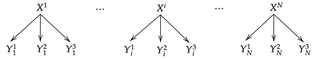
Figure 1. Illustration of the particle systems in coupled CBO model with $M=3$ particles for $Y$-system.

The particles $X^{i}_{\cdot}$, with $1\leq i\leq N$, are designed for the minimization problem

$$\min\limits_{x\in\mathbb{R}^{n}}F\big{(}x,\xi(x)\big{)},$$

where $\xi(\cdot)$ is a function that approximately captures the minimization problem (2.1) in a way that we will soon make precise. These particles follow a CBO scheme

$$\text{d}X^{i}_{t}=-\lambda_{1}\left(X^{i}_{t}-{z}(\widehat{\rho}_{X_{t}},\xi_{t}(X^{i}_{t}))\right)\,\text{d}t+\sigma_{1}D\left(X^{i}_{t}-{z}(\widehat{\rho}_{X_{t}},\xi_{t}(X^{i}_{t}))\right)\,\text{d}W^{X,i}_{t},$$

where $\lambda_{1},\sigma_{1}>0$ are constants, $X_{t}:=(X^{1}_{t},\dots,X^{N}_{t})\in\left(\mathbb{R}^{n}\right)^{N}$, and $\widehat{\rho}_{X_{t}}$ its corresponding empirical measure is

$$\widehat{\rho}_{X_{t}}=\frac{1}{N}\sum\limits_{i=1}^{N}\delta_{X^{i}_{t}}.$$

The weights functions are given by

(2.6) $$\omega_{\alpha}(x,y)=\exp(-\alpha F(x,y)),$$

for some $\alpha>0$ constant. We can then define the consensus point as

$${z}(\widehat{\rho}_{X_{t}},\xi_{t}(X^{i}_{t}))=\sum\limits_{k=1}^{N}X^{k}_{t}\frac{\omega_{\alpha}(X^{k}_{t},\xi_{t}(X^{i}_{t}))}{\sum\limits_{r=1}^{N}\omega_{\alpha}(X^{r}_{t},\xi_{t}(X^{i}_{t}))}=\int_{\mathbb{R}^{n}}x\frac{\omega_{\alpha}(x,\xi_{t}(X^{i}_{t}))}{\|\omega_{\alpha}(\cdot\,,\xi_{t}(X^{i}_{t}))\|_{L^{1}\left(\widehat{\rho}_{X_{t}}\right)}}\,\text{d}\widehat{\rho}_{X_{t}}(x).$$

The function $\xi_{t}(\cdot)$ is the coupling term between the $x$- and $y$-population of particles. It is given as follows

$$\xi_{t}(x)=\sum\limits_{j=1}^{M}Y^{j}_{x,t}\frac{\varpi_{\beta}(x,Y^{j}_{x,t})}{\sum\limits_{\ell=1}^{M}\varpi_{\beta}(x,Y^{\ell}_{x,t})}=\int_{\mathbb{R}^{m}}y\frac{\varpi_{\beta}(x,y)}{\|\varpi_{\beta}(x,\cdot)\|_{L^{1}\left(\widehat{\rho}_{Y_{x,t}}\right)}}\,\text{d}\widehat{\rho}_{Y_{x,t}}(y),$$

where we recall the weight function $\varpi_{\beta}(\cdot\,,\cdot)$ is defined in (2.4). This is in fact the consensus of the group of $y$-particles associated with each $x$-particle at time $t$. In other words, given a particle $X^{i}_{t}$, $1\leq i\leq N$, the consensus point at time $t$ for its corresponding population of $y$-particles $(Y^{1}_{i,t},\dots,Y^{M}_{i,t})$ is $\xi_{t}(X^{i}_{t})\in\mathbb{R}^{m}$ defined by

$$\xi_{t}(X^{i}_{t}) =\sum\limits_{j=1}^{M}Y^{j}_{i,t}\frac{\varpi_{\beta}(X^{i}_{t},Y^{j}_{i,t})}{\sum\limits_{\ell=1}^{M}\varpi_{\beta}(X^{i}_{t},Y^{\ell}_{i,t})}=\int_{\mathbb{R}^{m}}y\frac{\varpi_{\beta}(X^{i}_{t},y)}{\|\varpi_{\beta}(X^{i}_{t},\cdot\,)\|_{L^{1}\left(\widehat{\rho}_{Y_{i,t}}\right)}}\,\text{d}\widehat{\rho}_{Y_{i,t}}(y),$$

hence we have $\,\xi_{t}(X^{i}_{t})=\mathbf{v}(\widehat{\rho}_{Y_{i,t}},X^{i}_{t})\,$ where we recall $\mathbf{v}$ is defined in (2.5). For simplicity of notation, we shall denote it by

$$\mathbf{v}^{i}_{t}:=\mathbf{v}(\widehat{\rho}_{Y_{i,t}},X^{i}_{t}).$$

This means the consensus point ${z}$ takes the form

(2.7) $${z}(\widehat{\rho}_{X_{t}},\xi_{t}(X^{i}_{t})) =\sum\limits_{k=1}^{N}X^{k}_{t}\frac{\omega_{\alpha}(X^{k}_{t},\mathbf{v}(\widehat{\rho}_{Y_{i,t}},X^{i}_{t}))}{\sum\limits_{r=1}^{N}\omega_{\alpha}(X^{r}_{t},\mathbf{v}(\widehat{\rho}_{Y_{i,t}},X^{i}_{t}))}$$

$$=\int_{\mathbb{R}^{n}}x\frac{\omega_{\alpha}(x,\mathbf{v}(\widehat{\rho}_{Y_{i,t}},X^{i}_{t}))}{\|\omega_{\alpha}(\cdot\,,\mathbf{v}(\widehat{\rho}_{Y_{i,t}},X^{i}_{t}))\|_{L^{1}\left(\widehat{\rho}_{X_{t}}\right)}}\,\text{d}\widehat{\rho}_{X_{t}}(x)$$

$$=:\mathbf{z}(\widehat{\rho}_{X_{t}},\mathbf{v}^{i}_{t}).$$

Therefore, the dynamics are given by

(2.8) $$\text{d}X^{i}_{t}=-\lambda_{1}\left(X^{i}_{t}-\mathbf{z}(\widehat{\rho}_{X_{t}},\mathbf{v}^{i}_{t})\right)\,\text{d}t+\sigma_{1}D\left(X^{i}_{t}-\mathbf{z}(\widehat{\rho}_{X_{t}},\mathbf{v}^{i}_{t})\right)\,\text{d}W^{X,i}_{t},$$

and

(2.9) $$\mathbf{v}^{i}_{t}=\sum\limits_{j=1}^{M}Y^{j}_{i,t}\frac{\varpi_{\beta}(X^{i}_{t},Y^{j}_{i,t})}{\sum\limits_{\ell=1}^{M}\varpi_{\beta}(X^{i}_{t},Y^{\ell}_{i,t})}=\int_{\mathbb{R}^{m}}y\frac{\varpi_{\beta}(X^{i}_{t},y)}{\|\varpi_{\beta}(X^{i}_{t},\cdot\,)\|_{L^{1}\left(\widehat{\rho}_{Y_{i,t}}\right)}}\,\text{d}\widehat{\rho}_{Y_{i,t}}(y).$$

Note that the $X$-particles are interacting between each other, and each $X$-particle is also interacting with its corresponding $Y$-particles. But for any $1\leq i\leq N$, the particles $\{Y_{i,\cdot}^{j}\}_{j=1}^{M}$ associated to $X_{\cdot}^{i}$ do not interact with the particles $\{Y_{k,\cdot}^{j}\}_{j=1}^{M}$ for any $k\neq i$.

2.3. The multiscale CBO model

The presence of a hierarchical structure in the bi-level optimization problem, or in the order of optimization for min-max problems, suggests that the $x$- and $y$-particles are not at the same decision level. Indeed, while the $y$-particles perform optimization, the $x$-particles remain frozen, waiting for the $y$-particles to reach a steady-state. Numerically, this means that for each element of the $x$-population, we update its corresponding $y$-population for several time steps before we update the $x$-population. In other words, the evolution of $y$-population is on a faster time-scale than the $x$-population. This distinction motivates the introduction of two time scales.

The multi-time scaling of such coupled systems of SDEs can be modeled with singular perturbation, that is, given some small parameter $0<\varepsilon\ll 1$, we consider the following dynamics:

(2.10) $$\left\{\;\begin{aligned} &\text{d}X^{i}_{t}=-\lambda_{1}\left(X^{i}_{t}-\mathbf{z}(\widehat{\rho}_{X_{t}},\mathbf{v}^{i}_{t})\right)\,\text{d}t+\sigma_{1}D\left(X^{i}_{t}-\mathbf{z}(\widehat{\rho}_{X_{t}},\mathbf{v}^{i}_{t})\right)\,\text{d}W^{X,i}_{t}\\ &\text{d}Y^{j}_{i,t}=-\frac{1}{\varepsilon}\lambda_{2}\left(Y^{j}_{i,t}-\mathbf{v}^{i}_{t}\right)\,\text{d}t+\sqrt{\frac{1}{\varepsilon}}\sigma_{2}D\left(Y^{j}_{i,t}-\mathbf{v}^{i}_{t}\right)\,\text{d}W^{Y,j}_{i,t}\\ &\text{Given }\,(X^{i}_{0},Y^{j}_{i,0}),\quad\quad 1\leq j\leq M,\quad 1\leq i\leq N,\quad 0\leq t\leq T,\end{aligned}\right.$$

where $\mathbf{v}^{M}_{i,t}$ defined in (2.9) is a function of $(X^{i}_{t},Y_{i,t}^{1},\dots\,,Y_{i,t}^{M})$, and and $\mathbf{z}(\cdot\,,\cdot\,)$ is defined in (2.7).

The $x$-processes are referred to as the slow dynamics, while the $y$-processes are the fast dynamics. This denomination can be justified as follows. Let us change the time variable using $\tau=t/\varepsilon$. The system (2.10) becomes

$$\left\{\;\begin{aligned} &\text{d}\widetilde{X}^{i}_{\tau}=-\varepsilon\,\lambda_{1}\left(\widetilde{X}^{i}_{\tau}-\mathbf{z}(\widehat{\rho}_{\widetilde{X}_{\tau}},\mathbf{v}^{i}_{\tau})\right)\,\text{d}\tau+\sqrt{\varepsilon}\,\sigma_{1}D\left(\widetilde{X}^{i}_{\tau}-\mathbf{z}(\widehat{\rho}_{\widetilde{X}_{\tau}},\mathbf{v}^{i}_{\tau})\right)\,\text{d}\widetilde{W}^{X,i}_{\tau}\\ &\text{d}\widetilde{Y}^{j}_{i,\tau}=-\lambda_{2}\left(\widetilde{Y}^{j}_{i,\tau}-\mathbf{v}^{i}_{\tau}\right)\,\text{d}\tau+\sigma_{2}D\left(\widetilde{Y}^{j}_{i,\tau}-\mathbf{v}^{i}_{\tau}\right)\,\text{d}\widetilde{W}^{Y,j}_{i,\tau}\\ &\text{Given }\,(\widetilde{X}^{i}_{0},\widetilde{Y}^{j}_{i,0}),\quad\quad 1\leq j\leq M,\quad 1\leq i\leq N,\end{aligned}\right.$$

where we use the notation $\widetilde{Z}_{\tau}=Z_{\varepsilon\tau}$, for $Z_{\cdot}=X^{i}_{\cdot},Y^{j}_{i,\cdot}$, and $\widetilde{W}^{X,i}_{\tau}=(1/\sqrt{\varepsilon})W^{X,i}_{\varepsilon\tau}$, $\widetilde{W}^{Y,j}_{i,\tau}=(1/\sqrt{\varepsilon})W^{Y,j}_{i,\varepsilon\tau}$. Thus it can be seen that when $\varepsilon$ is small, the processes $\widetilde{X}^{i}_{\tau}$ tend to be frozen compared to the evolution of $\widetilde{Y}^{j}_{i,\tau}$. In other words, by the time the processes $\widetilde{X}^{i}_{\tau}$ make a significant change in their evolution, the processes $\widetilde{Y}^{j}_{i,\tau}$ would have already reached their long-time steady state. This steady-state behavior should be captured by their invariant measure under suitable recurrence condition. The treatment (both in theory and practice) of two-scale dynamics of this type is a challenging task. This motivates the introduction of simplified dynamics obtained by passing to the limit $\varepsilon\to 0$ in (2.10). Indeed, in this case, one obtains a system consisting only of the slow component of (2.10), whose dynamics is averaged with respect to the invariant measure of the fast component, as it will be explained in more detail in the next section. This phenomenon is known as the averaging principle and is the core idea behind singular perturbations and homogenization. In the context of optimization, singular perturbations of SDEs have been used in [chaudhari2018deep] which was then extended to a more general setting in [bardi2023singular, bardi2022deep] where a control parameter have been introduced, playing the role of a controlled learning rate.

A particular advantage of the latter is that it also plays the role of a model reduction technique: from a system consisting of two components (the $x$- and $y$-particles), we obtain a system of a single component (the modified $x$-particles). On the other hand, a challenge associated to the averaging method is that it requires the (explicit) computation of the invariant measure of the fast process (the $y$-particles). In practice, we shall bypass this obstacle by substituting the average with respect to the invariant measure (which is an average in space) by the average with respect to time. This is possible due to ergodicity of the $y$-particles, as established by the celebrated Birkhoff’s ergodic theorem.

Although the averaging principle has been intensively studied since decades, to the best of our knowledge, the system described in (2.10) does not satisfy the assumptions in the very recent developments of the averaging principle (see for example [hong2023central, hong2022strong, rockner2021strong, li2022near] and the references therein). Further modifications are thus needed, which is the object of the next section.

3. Implementation and convergence of the CBO model with effective dynamics

3.1. The modified multiscale CBO model

Before formalizing the modified multiscale CBO model, we shall introduce some notations. Given $R>0$ fixed, we define for $\forall\,v=(v_{k})_{1\leq k\leq d}\in\mathbb{R}^{d}$, two truncation functions

$$\phi_{R}(v)=\big{(}\min\{|v_{k}|,R\}\big{)}_{1\leq k\leq d}\,\in\mathbb{R}^{d},$$

$$\psi_{R}(v)=\big{(}\psi_{R}(v)_{k}\big{)}_{1\leq k\leq d},\quad\text{ where }\psi_{R}(v)_{k}=\left\{\;\begin{aligned} &v_{k}\;,\quad\quad\text{ if }\;|v_{k}|\leq R\\ &\frac{v_{k}}{|v_{k}|}R\;,\quad\text{ if }\;|v_{k}|>R\end{aligned}\right..$$

Then, we define a matrix-valued function

$$\forall\,v\in\mathbb{R}^{d},\quad D^{\delta}_{R}(v)=\text{diag}(\delta+\phi_{R}(v))\in\mathbb{R}^{d\times d},$$

where as before, $\text{diag}(\cdot)$ is the diagonal matrix whose components are the elements of the vector to which it is applied, e.g., the $k$-th element in the diagonal of $D^{\delta}_{R}(v)$ is $\delta+\min\{|v_{k}|,R\}>0$. In particular $D^{\delta}_{R}(\cdot)$ is a positive definite matrix. We shall keep the same notation $\phi_{R},\psi_{R},D^{\delta}_{R}$ regardless of the dimension $d$, as it will be clear from the context. We then define a matrix-valued function

$$\forall\,M_{1},\dots,M_{k}\in\mathbb{R}^{d\times d},\quad\mathbb{D}(M_{1},\dots,M_{k})=\text{Diag}(M_{1},\dots,M_{k}),$$

where $\text{Diag}(\cdot)$ is the block-diagonal matrix whose diagonal blocks are the matrices $M_{1},\dots,M_{k}$. In particular, we define

$$\forall\,v^{1},\dots,v^{k}\in\mathbb{R}^{d},\quad\mathbb{D}^{\delta}_{R}(v^{1},\dots,v^{k})=\mathbb{D}(D^{\delta}_{R}(v^{1}),\dots,D^{\delta}_{R}(v^{k})).$$

This is a block-diagonal matrix in $\mathbb{R}^{dk\times dk}$. Each of its $j$-th block ($1\leq j\leq k$) is a diagonal matrix whose diagonal components are $\delta+\min\{|v_{i}^{j}|,R\}$ with $1\leq i\leq d$. To keep the notation concise in what follows, let us denote the state vector of the particle system using the notation

$$\mathds{X}=\big{(}\mathbf{X}_{i}\big{)}_{1\leq i\leq N}\in\mathbb{R}^{nN},\quad\text{ where }\mathbf{X}_{i}\in\mathbb{R}^{n},$$

$$\mathds{Y}=(\mathbf{Y}_{i})_{1\leq i\leq N}\in\mathbb{R}^{mMN},\quad\text{ where }\mathbf{Y}_{i}=(Y^{j}_{i})_{1\leq j\leq M}\in\mathbb{R}^{mM},\quad\text{ and }Y^{j}_{i}\in\mathbb{R}^{m}.$$

The finite dimensional system of singularly perturbed SDEs is stated as follows:

(3.1) $$\left\{\;\begin{aligned} &\text{d}\mathds{X}_{t}=\mathscr{F}(\mathds{X}_{t},\mathds{Y}_{t})\,\text{d}t+\mathscr{G}(\mathds{X}_{t},\mathds{Y}_{t})\,\text{d}\mathds{W}^{1}_{t}\\ &\text{d}\mathds{Y}_{t}=\frac{1}{\varepsilon}\mathscr{B}(\mathds{X}_{t},\mathds{Y}_{t})\,\text{d}t+\frac{1}{\sqrt{\varepsilon}}\mathscr{H}(\mathds{X}_{t},\mathds{Y}_{t})\,\text{d}\mathds{W}^{2}_{t}\\ &\mathds{X}_{0}=\mathbf{x}_{0}\in\mathbb{R}^{nN},\quad\text{ and }\quad\mathds{Y}_{0}=\mathbf{y}_{0}\in\mathbb{R}^{mMN},\end{aligned}\right.$$

where $\mathds{W}^{1}_{\cdot}$ and $\mathds{W}^{2}_{\cdot}$ are $nN$, $mMN$-dimensional independent standard Brownian motions. The coefficients in (3.1) are defined as follows.

3.1.1. The drift $\mathscr{B}$ in $\mathds{Y}$-process

The drift term of the fast process $\{\mathds{Y}_{t}\}_{t\geq 0}$ is given by

$$\mathscr{B}(\mathds{X},\mathds{Y})=\big{(}B(\mathbf{X}_{i},\mathbf{Y}_{i})\big{)}_{1\leq i\leq N},\quad\text{ where }\quad B(\mathbf{X}_{i},\mathbf{Y}_{i})=\big{(}b_{i}^{j}(\mathbf{X}_{i},\mathbf{Y}_{i})\big{)}_{1\leq j\leq M}$$

and

$$b_{i}^{j}(\mathbf{X}_{i},\mathbf{Y}_{i}) =-\lambda_{2}\,\psi_{R_{2}}\left(\,Y_{i}^{j}-c\,\sum_{k=1}^{M}Y_{i}^{k}\frac{\varpi_{\beta}\left(\mathbf{X}_{i},Y_{i}^{k}\right)}{\sum_{\ell=1}^{M}\varpi_{\beta}\left(\mathbf{X}_{i},Y_{i}^{\ell}\right)}\,\right)\in\mathbb{R}^{m},$$

where $c$ is a positive constant that will be needed later in Theorem 3.1. It guarantees the validity of a recurrence condition which ultimately ensures ergodicity of the process, i.e. existence and uniqueness of its invariant measure (see point (iii) in the proof of Theorem 3.1 in Appendix A). Therefore we have

$$b_{i}^{j}(\mathbf{X}_{i},\mathbf{Y}_{i})\in\mathbb{R}^{m},\quad B(\mathbf{X}_{i},\mathbf{Y}_{i})\in\mathbb{R}^{mM}\quad\text{ and }\quad\mathscr{B}(\mathds{X},\mathds{Y})\in\mathbb{R}^{mMN}.$$

Note that, using $\psi_{R_{2}}$, the drift functions $b_{i}^{j}$ take values in balls of radius $\lambda_{2}R_{2}$.

3.1.2. The diffusion $\mathscr{H}$ in $\mathds{Y}$-process

The diffusion term of the fast process $\{\mathds{Y}_{t}\}_{t\geq 0}$ is given by

$$\mathscr{H}(\mathds{X},\mathds{Y}) =\text{Diag}\left(\{H(\mathbf{X}_{i},\mathbf{Y}_{i})\}_{1\leq i\leq N}\right),$$

$$\text{where }\;H(\mathbf{X}_{i},\mathbf{Y}_{i}) =\sigma_{2}\,\mathbb{D}^{\delta_{2}}_{R_{2}}\left(\{h_{i}^{j}(\mathbf{X}_{i},\mathbf{Y}_{i})\}_{1\leq j\leq M}\right),$$

and, similar to $b_{i}^{j}$, we have

$$h_{i}^{j}(\mathbf{X}_{i},\mathbf{Y}_{i}) =Y_{i}^{j}-c\,\sum_{k=1}^{M}Y_{i}^{k}\frac{\varpi_{\beta}\left(\mathbf{X}_{i},Y_{i}^{k}\right)}{\sum\limits_{\ell=1}^{M}\varpi_{\beta}\left(\mathbf{X}_{i},Y_{i}^{\ell}\right)}\in\mathbb{R}^{m}.$$

Therefore we have

$$h_{i}^{j}(\mathbf{X}_{i},\mathbf{Y}_{i})\in\mathbb{R}^{m},\quad H(\mathbf{X}_{i},\mathbf{Y}_{i})\in\mathbb{R}^{mM\times mM},\quad\text{ and}\quad\mathscr{H}(\mathds{X},\mathds{Y})\in\mathbb{R}^{mMN\times mMN}.$$

Note that, using $\mathds{D}^{\delta_{2}}_{R_{2}}$, the diffusion functions $H$ take values in balls of radius $\sigma_{2}R_{2}$.

3.1.3. The drift $\mathscr{F}$ in $\mathds{X}$-process

The drift term of the slow process $\{\mathds{X}_{t}\}_{t\geq 0}$ is given by

$$\mathscr{F}(\mathds{X},\mathds{Y}) =\big{(}F_{i}(\mathds{X},\mathbf{Y}_{i})\big{)}_{1\leq i\leq N}$$

$$\text{and }\;F_{i}(\mathds{X},\mathbf{Y}_{i}) =-\lambda_{1}\,\psi_{R_{1}}\left(\mathbf{X}_{i}-\sum\limits_{k=1}^{N}\mathbf{X}_{k}\frac{\omega_{\alpha}\left(\mathbf{X}_{k},\frac{1}{c}\mathbf{v}^{i}\right)}{\sum\limits_{r=1}^{N}\omega_{\alpha}\left(\mathbf{X}_{r},\frac{1}{c}\mathbf{v}^{i}\right)}\right),$$

where we recall

$$\mathbf{v}^{i}=\sum\limits_{j=1}^{M}Y^{j}_{i}\frac{\varpi_{\beta}(X_{i},Y^{j}_{i})}{\sum\limits_{\ell=1}^{M}\varpi_{\beta}(X_{i},Y^{\ell}_{i})}.$$

Therefore we have

$$F_{i}(\mathds{X},\mathbf{Y}_{i})\in\mathbb{R}^{n}\quad\text{ and }\quad\mathscr{F}(\mathds{X},\mathds{Y})\in\mathbb{R}^{nN}.$$

Note that, using $\psi_{R_{1}}$, the drift functions $F_{i}$ take values in balls of radius $\lambda_{1}R_{1}$.

3.1.4. The diffusion $\mathscr{G}$ in $\mathds{X}$-process

The diffusion term of the slow process $\{\mathds{X}_{t}\}_{t\geq 0}$ is given by

$$\mathscr{G}(\mathds{X},\mathds{Y})=\sigma_{1}\,\mathds{D}^{\delta_{1}}_{R_{1}}\left(\{G_{i}(\mathds{X},\mathbf{Y}_{i})\}_{1\leq i\leq N}\right)$$

and, similar to $F_{i}$, we have

$$G_{i}(\mathds{X},\mathbf{Y}_{i})=\mathbf{X}_{i}-\sum\limits_{k=1}^{N}\mathbf{X}_{k}\frac{\omega_{\alpha}\left(\mathbf{X}_{k},\frac{1}{c}\mathbf{v}^{i}\right)}{\sum\limits_{r=1}^{N}\omega_{\alpha}\left(\mathbf{X}_{r},\frac{1}{c}\mathbf{v}^{i}\right)}.$$

Therefore we have

$$G_{i}(\mathds{X},\mathbf{Y}_{i})\in\mathbb{R}^{n}\quad\text{ and }\quad\mathscr{G}(\mathds{X},\mathds{Y})\in\mathbb{R}^{nN\times nN}.$$

Note that, using $\mathds{D}^{\delta_{1}}_{R_{1}}$, the diffusion function $\mathscr{G}$ takes values in a unit ball of radius $\sigma_{1}R_{1}$.

Remark 3.1.

The following are some relevant observations regarding the proposed multiscale CBO model.

1. Without loss of generality, one could consider $R_{1}=R_{2}=:R$, with $R<\infty$ sufficiently large, because the CBO algorithm works in practice over a compact domain, for example an Euclidean ball $\mathcal{B}_{0}(\bar{R})$ centered in $0$ with radius $\bar{R}$, which contains the initial position of the particles. Therefore, if the truncation parameter $R$ is chosen large enough, i.e., $R\gg\bar{R}$, the truncation function is essentially $\phi_{R}(v)=(|v_{k}|)_{1\leq k\leq d}$ since the particles are unlikely to leave a neighborhood of $\mathcal{B}_{0}(\bar{R})$. It is also worth mentioning that a CBO algorithm with a truncated noise has been studied in [fornasier2023consensus].

2. The parameters $\delta_{1},\delta_{2}$ are chosen to be small constants. In particular, one could set $\delta_{1}=\delta_{2}=:\delta>0$. They ensure the diffusion matrix remains positive definite, providing enough noise to prevent the dynamics from collapsing to one point very quickly. Numerically, this still allows the particles to converge to a small neighborhood around the global optimizer.

3. The initial condition being deterministic is necessary for our model in order to justify the limit $\varepsilon\to 0$, as we will do in the next section, and in regard to the existing literature on this topic. Nonetheless, it should be noted that, when implemented numerically, the CBO model is able to perform well with random initialization as it is customary done in CBO methods.

3.2. The effective CBO and the averaging principle

At the limit $\varepsilon\to 0$, we obtain averaged (effective) dynamics, where the dynamics associated to $\mathds{Y}$ disappear and the dynamics of $\mathds{X}$ are averaged with respect to the limiting (ergodic) behavior of $\mathds{Y}$. This yields an effective CBO model which corresponds to the macro-scale dynamics governed by

(3.2) $$\text{d}\hat{\mathds{X}}_{t}=\overline{\mathscr{F}}(\hat{\mathds{X}}_{t})\,\text{d}t+\overline{\mathscr{G}}(\hat{\mathds{X}}_{t})\,\text{d}\mathds{W}^{1}_{t},\quad\hat{\mathds{X}}_{0}=\mathbf{x}_{0}\in\mathbb{R}^{nN}.$$

The new averaged coefficients are given by

$$\overline{\mathscr{F}}(x):=\int\mathscr{F}(x,y)\,\Upsilon_{x}(\text{d}y)\;\text{ and }\;\overline{\mathscr{G}}(x):=\sqrt{\int\mathscr{G}(x,y)\mathscr{G}^{*}(x,y)\,\Upsilon_{x}(\text{d}y)},$$

the two integrals are defined on $\mathbb{R}^{mMN}\ni y$, where $y$ is a mute variable, and the averaged coefficients are functions of $x\in\mathbb{R}^{nN}$. Here, $\Upsilon_{x}$ is the unique invariant probability measure for the dynamics $\mathds{Y}^{x}_{\cdot}$ solution to the frozen equation

(3.3) $$\text{d}\mathds{Y}^{x}_{t}=\frac{1}{\varepsilon}\mathscr{B}(x,\mathds{Y}^{x}_{t})\,\text{d}t+\frac{1}{\sqrt{\varepsilon}}\mathscr{H}(x,\mathds{Y}^{x}_{t})\,\text{d}\mathds{W}^{2}_{t},\quad\mathds{Y}^{x}_{0}=\mathbf{y}_{0}\in\mathbb{R}^{mMN},$$

where we have arbitrarily fixed $x\in\mathbb{R}^{nN}$. This corresponds to the dynamics of the fast process $\mathds{Y}$, where we have frozen the slow process $\mathds{X}$ to some value $x$. To avoid any confusion, let us once again explicitly rewrite the dynamics (3.2)

$$\text{d}\hat{\mathds{X}}_{t}=\int\mathscr{F}(\hat{\mathds{X}}_{t},y)\,\Upsilon_{\hat{\mathds{X}}_{t}}(\text{d}y)\;\text{d}t+\sqrt{\int\mathscr{G}(\hat{\mathds{X}}_{t},y)\mathscr{G}^{*}(\hat{\mathds{X}}_{t},y)\,\Upsilon_{\hat{\mathds{X}}_{t}}(\text{d}y)}\;\,\text{d}\mathds{W}^{1}_{t}.$$

In other words, the system (3.1), whose dimension is $nN\times mMN$, reduces to (3.2), whose dimension is $nN$.

The convergence of the slow component $\mathds{X}$ in (3.1) to the process $\hat{\mathds{X}}$ in (3.2) has been studied for decades, yet many open questions still persist. In our setting, we will show that the convergence is guaranteed with the recent results in [rockner2021diffusion] (see also [rockner2019strong, Theorem 2.5]), provided the constant $c$ in Section 3.1.1 is small. We shall denote by $C_{b}^{2+\theta}$, with $\theta\in(0,1)$, the set of bounded and $C^{2}$ functions whose second order derivatives are locally Hölder continuous with exponent $\theta$.

Theorem 3.1.

Let $T>0$ and $\theta\in(0,1)$. Then for $c\in(0,1)$ small, we have

$$\sup_{t\in[0,T]}\left|\mathbb{E}\left[\varphi(\mathds{X}_{t}^{\varepsilon})\right]-\mathbb{E}[\varphi(\hat{\mathds{X}}_{t})]\right|\leqslant C_{T}\,\varepsilon^{\frac{\theta}{2}},\quad\forall\,\varphi\in C_{b}^{2+\theta}(\mathbb{R}^{nN}),$$

where $C_{T}>0$ is a constant independent of $\varepsilon$.

The proof of the theorem is postponed to Appendix A.

Remark 3.2.

We can choose $\theta\in(0,2]$, provided that we smoothen the truncation functions (used in (3.1)) using mollifiers, as it is customary. In practice, this will not alter the numerical results. Yet we refrain from doing it in the present manuscript as it will make the presentation less readable.

3.3. The algorithm

We propose an algorithm which approximates the computation of the effective (averaged) dynamics $\hat{\mathds{X}}_{\cdot}$ in (3.2). Without loss of generality, we assume the parameter $R_{1}$ of the truncation functions used in the drift $\mathscr{F}$ and in the diffusion $\mathscr{G}$ is sufficiently large, so that the truncation functions are in fact the identity. This will simplify the computation of the averaged quantities $\overline{\mathscr{F}}$ and $\overline{\mathscr{G}}$. Indeed, in this case, we have $\mathscr{F}(\mathds{X},\mathds{Y})=\big{(}F_{i}(\mathds{X},\mathbf{Y}_{i})\big{)}_{1\leq i\leq N}$ and $F_{i}(\mathds{X},\mathbf{Y}_{i})=-\lambda_{1}\,\left(\mathbf{X}_{i}-\mathbf{z}(\mathds{X},c^{-1}\mathbf{v}^{i})\right)$, where

$$\mathbf{z}(\mathds{X},c^{-1}\mathbf{v}^{i})=\sum\limits_{k=1}^{N}\mathbf{X}_{k}\frac{\omega_{\alpha}\left(\mathbf{X}_{k},\frac{1}{c}\mathbf{v}^{i}\right)}{\sum\limits_{r=1}^{N}\omega_{\alpha}\left(\mathbf{X}_{r},\frac{1}{c}\mathbf{v}^{i}\right)}\text{ and }\mathbf{v}^{i}=\sum\limits_{j=1}^{M}Y^{j}_{i}\frac{\varpi_{\beta}(X_{i},Y^{j}_{i})}{\sum\limits_{\ell=1}^{M}\varpi_{\beta}(X_{i},Y^{\ell}_{i})}.$$

Its averaged analogue is obtained as $\overline{\mathscr{F}}(\mathds{X})=\big{(}\overline{F}_{i}(\mathds{X})\big{)}_{1\leq i\leq N}$ and

$$\overline{F}_{i}(\mathds{X})=-\lambda_{1}\,\int\left(\mathbf{X}_{i}-\mathbf{z}(\mathds{X},c^{-1}\mathbf{v}^{i})\right)\,\text{d}\Upsilon_{\mathds{X}}^{i}=-\lambda_{1}\left(\mathbf{X}_{i}-\int\mathbf{z}(\mathds{X},c^{-1}\mathbf{v}^{i})\,\text{d}\Upsilon_{\mathds{X}}^{i}\right),$$

where we recall $\mathbf{v}^{i}\equiv\mathbf{v}^{i}(\mathbf{Y}_{i})$ is a function of $\mathbf{Y}_{i}\in\mathbb{R}^{mM}$, and $\text{d}\Upsilon_{\mathds{X}}$ defined in the previous section is expressed as a product measure $\text{d}\Upsilon_{\mathds{X}}(y)=\bigotimes\limits_{i=1}^{N}\Upsilon_{\mathds{X}}^{i}(\text{d}y_{i})$ for $y\in\mathbb{R}^{mMN}$ and $y=(y_{i})_{1\leq i\leq N}$. Therefore, the goal is to estimate the averaged consensus point given

(3.4) $$\overline{\mathbf{z}}_{i}(\mathds{X}):=\int_{\mathbb{R}^{mM}}\mathbf{z}(\mathds{X},c^{-1}\mathbf{v}^{i}(y_{i}))\,\Upsilon_{\mathds{X}}^{i}(\text{d}y_{i}).$$

This is done using the relationship between the invariant measure and the averaged long-time behavior:

(3.5) $$\int_{\mathbb{R}^{mM}}\mathbf{z}(\mathds{X},c^{-1}\mathbf{v}^{i}(y_{i}))\,\Upsilon_{\mathds{X}}^{i}(\text{d}y_{i})=\lim\limits_{T\to+\infty}\frac{1}{T}\int_{0}^{T}\mathbf{z}(\mathds{X},c^{-1}\mathbf{v}^{i}(\mathbf{Y}_{i,t}))\,\text{d}t,$$

where $\mathbf{Y}_{i}$ solves (3.3) with $x=\mathds{X}$ is a fixed parameter therein.

For the diffusion term, instead of computing $\overline{\mathscr{G}}$ as defined in the previous subsection, we shall approximate it with a diagonal matrix whose elements are the components of the vector

$$\sigma_{1}\left(\delta+\big{|}\mathbf{X}_{i}-\overline{\mathbf{z}}_{i}(\mathds{X})\big{|}\right).$$

Here, we use the notation $|v|=(|v_{i}|)_{1\leq i\leq d}$, for any vector $v\in\mathbb{R}^{d}$, and the constant $\delta$ is a vector of the same dimension whose elements are all equal to $\delta$.

Thus, at each iteration of the algorithm, we would like to retrieve a quantity that becomes closer to $\overline{\mathbf{z}}_{i}(\mathds{X})$ as defined in (3.4), using the averaging in time as in the right-hand side of (3.5). We proceed in a similar fashion as [chaudhari2019entropy, Algorithm 1], using a forward-looking averaging (instead of a linear averaging), that is:

1. we compute $\overline{\mathbf{z}}_{i}(\mathds{X})$ at time step $t+1$ as a convex combination of its value at the previous step $t$, and the value of $\mathbf{z}(\mathds{X},c^{-1}\mathbf{v}^{i})$ at time step $t+1$; see the forward looking averaging (FLA) step in Algorithm 1 below.

Note that the computation of the invariant measure could be improved and/or realized differently, for example using the results in [alrachid2019new].
In the following, we present the pseudo-code for multiscale CBO solving the bi-level optimization problem (1.1).

Set parameters: $\gamma,\,\alpha,\,\beta,\,\lambda_{1},\,\lambda_{2},\,\sigma_{1},\,\sigma_{2},\,\Delta t,\,\Delta\tau,\,T_{x},\,T_{y},\,R_{1},\,R_{2},\,\delta_{1},\,\delta_{2}\,,c\;$;

Initialize: $\mathbf{z}^{i}_{0}=X_{0}^{i}\sim\rho_{0},\;i=1,\ldots,N\;$;

     $Y^{j}_{i,0}\sim\mu_{0},\;j=1,\ldots,M$, where $M\ll N$;

     $t=0$, $\mathcal{T}_{x}=T_{x}/\Delta t$, $\mathcal{T}_{y}=T_{y}/\Delta\tau$;

while $t\leq\mathcal{T}_{x}$  do

       for $i=1,\ldots,N$ do

             $\tau=0$;

             $\mathbf{v}^{i}_{\tau}=\sum\limits_{j=1}^{M}Y^{j}_{i,\tau}\frac{\varpi_{\beta}(X^{i}_{t},Y^{j}_{i,\tau})}{\sum\limits_{\ell=1}^{M}\varpi_{\beta}(X^{i}_{t},Y^{\ell}_{i,\tau})}$ ;

              /* Initial consensus of $\mathbf{Y}_{i,0}$ */

             while $\tau\leq\mathcal{T}_{y}$ do

                   for $j=1,\ldots,M$ do

                         sample $W_{i,\tau}^{Y,j}$ from $\mathcal{N}(0,\Delta\tau\,\mathds{I}_{m})$;

                         $Y^{j}_{i,\tau}\leftarrow Y^{j}_{i,\tau}-\lambda_{2}\psi_{R_{2}}\!\left(Y^{j}_{i,\tau}-c\,\mathbf{v}^{i}_{\tau}\right)\Delta\tau+\sigma_{2}D_{R_{2}}^{\delta_{2}}\!\left(Y^{j}_{i,\tau}-c\,\mathbf{v}^{i}_{\tau}\right)W_{i,\tau}^{Y,j}$;

                        

                   end for

                  $\mathbf{v}^{i}_{\tau}\leftarrow\sum\limits_{j=1}^{M}Y^{j}_{i,\tau}\frac{\varpi_{\beta}(X^{i}_{t},Y^{j}_{i,\tau})}{\sum\limits_{\ell=1}^{M}\varpi_{\beta}(X^{i}_{t},Y^{\ell}_{i,\tau})}$ ;

                    /* consensus of $\mathbf{Y}_{i,\tau}$ */

                   $\mathbf{z}^{\prime}\leftarrow\sum\limits_{k=1}^{N}X^{k}_{t}\frac{\omega_{\alpha}(X^{k}_{t},\frac{1}{c}\mathbf{v}^{i}_{\tau})}{\sum\limits_{r=1}^{N}\omega_{\alpha}(X^{r}_{t},\frac{1}{c}\mathbf{v}^{i}_{\tau})}$ ;

                    /* auxiliary variable */

                   $\mathbf{z}^{i}_{t}\leftarrow(1-\gamma)\mathbf{z}^{i}_{t}+\gamma\mathbf{z}^{\prime}$ ;

                    /* FLA of $X^{i}_{t}$; depends on $i$ */

                   $\tau\leftarrow\tau+1$;

                  

             end while

            sample $W_{i,t}^{X}$ from $\mathcal{N}(0,\Delta t\,\mathds{I}_{n})$;

             $X^{i}_{t}\leftarrow X^{i}_{t}-\lambda_{1}\psi_{R_{1}}\left(X_{t}^{i}-\mathbf{z}^{i}_{t}\right)\Delta t+\sigma_{1}D_{R_{1}}^{\delta_{1}}\left(X_{t}^{i}-\mathbf{z}^{i}_{t}\right)W_{i,t}^{X}$ ;

            

       end for

      $t\leftarrow t+1$;

      

end while

$(\bar{X},\,\bar{\mathbf{v}})\leftarrow\left(\frac{1}{N}\sum_{i=1}^{N}X_{\mathcal{T}_{x}}^{i},\;\frac{1}{N}\sum_{i=1}^{N}\mathbf{v}_{\mathcal{T}_{y}}^{i}\right)$;

$X^{*}\leftarrow\sum\limits_{k=1}^{N}X_{\mathcal{T}_{x}}^{k}\frac{\omega_{\alpha}\left(X_{\mathcal{T}_{x}}^{k},\frac{1}{c}\bar{\mathbf{v}}\right)}{\sum\limits_{r=1}^{N}\omega_{\alpha}\left(X_{\mathcal{T}_{x}}^{r},\frac{1}{c}\bar{\mathbf{v}}\right)}$;

$Y^{*}\leftarrow\frac{1}{c}\sum\limits_{k=1}^{N}\mathbf{v}_{\mathcal{T}_{y}}^{k}\frac{\varpi_{\beta}\left(\bar{X},\,\frac{1}{c}\mathbf{v}_{\mathcal{T}_{y}}^{k}\right)}{\sum\limits_{r=1}^{N}\varpi_{\beta}\left(\bar{X},\,\frac{1}{c}\mathbf{v}_{\mathcal{T}_{y}}^{r}\right)}$;

Return $(X^{*},Y^{*})$ ;

  /* Approximation of solution to (1.1) */

Algorithm 1 multiscale CBO for bi-level optimization problems

In Algorithm 1, the weight function are defined according to the objective functions of upper and lower level optimization problems (see (2.4)-(2.6)), i.e.,

$$\varpi_{\beta}(x,y)=\exp(-\beta G(x,y))\quad\text{and}\quad\omega_{\alpha}(x,y)=\exp(-\alpha F(x,y)).$$

Remark 3.3.

It is important to note that for running Algorithm 1, we do not need to have as many $y$-particles as $x$-particles, in particular we have $M\ll N$. Moreover, it is not necessary to run the dynamics of the $y$-particles for a long time, that is, an approximate value of their consensus is already enough for the algorithm to perform well. Hence, we can choose $T_{y}\ll T_{x}$. This can be justified by the fact that errors in the computation of the consensus for the $y$-particles, can be tamed during the averaging procedure used for computing the consensus of the $x$-particles. On the other hand, the for loop can be computed in parallel, since the groups of particles $\mathbf{Y}_{i}=\{Y_{i}^{1},\cdots,Y_{i}^{M}\}$ are independent from $\mathbf{Y}_{k}$ for any $k\neq i$.

Remark 3.4.

Although Theorem 3.1 establishes the convergence of the model (3.1) to an averaged dynamics as $\varepsilon\rightarrow 0$ under the assumption $c\in(0,1)$ small, numerical results suggest that this smallness assumption is not necessary for the convergence to hold. Indeed, in practice (see Algorithm 1), we implement an approximation of the averaging with respect to the invariant measure which mimics the dynamics with a finite $\varepsilon$. See the discussion at the beginning of Section 3.3. Hence we can simply set $c=1$, and obtain satisfactory accuracy in numerical experiments.

4. Multiscale CBO for multi-level optimization

4.1. The general strategy

The bi-level approach presented in the previous sections can be extended to tackle multi-level optimization problems of the form

(4.1) $$\min\limits_{x_{0}\in\mathbb{R}^{d_{0}}}\;F_{0}(x_{0},y_{1},\dots,y_{n})$$

$$\quad\quad\text{ s.t. }\;y_{1}\in\operatorname*{argmin}\limits_{y\in\mathbb{R}^{d_{1}}}F_{1}(x_{0},y,y_{2},\dots,y_{n})$$

$$\quad\quad\quad\quad\text{ s.t. }\;y_{2}\in\operatorname*{argmin}\limits_{y\in\mathbb{R}^{d_{2}}}\;F_{2}(x_{0},y_{1},y,y_{3},\dots,y_{n})$$

$$\quad\quad\quad\quad\quad\quad\quad\ddots\quad\quad\quad\quad\ddots$$

$$\quad\quad\quad\quad\quad\quad\quad\quad\text{ s.t. }\;y_{n}\in\operatorname*{argmin}\limits_{y\in\mathbb{R}^{d_{n}}}\;F_{n}(x_{0},\dots,y_{n-1},y)$$

In this case, the multiscale CBO model would have as many scales as the number of levels in (4.1). Its system of interacting SDEs is analogous to (3.1), that is

(4.2) $$\left\{\;\begin{aligned} &\text{d}\mathds{X}_{t}=\mathscr{F}(\mathds{X}_{t},\mathds{Y}^{1}_{t},\dots,\mathds{Y}^{n}_{t})\,\text{d}t+\mathscr{G}(\mathds{X}_{t},\mathds{Y}^{1}_{t},\dots,\mathds{Y}^{n}_{t})\,\text{d}\mathds{W}^{0}_{t}\\ &\text{d}\mathds{Y}^{1}_{t}=\frac{1}{\varepsilon}\mathscr{B}_{1}(\mathds{X}_{t},\mathds{Y}^{1}_{t},\dots,\mathds{Y}^{n}_{t})\,\text{d}t+\frac{1}{\sqrt{\varepsilon}}\mathscr{H}_{1}(\mathds{X}_{t},\mathds{Y}^{1}_{t},\dots,\mathds{Y}^{n}_{t})\,\text{d}\mathds{W}^{1}_{t}\\ &\quad\quad\;\vdots\\ &\text{d}\mathds{Y}^{n}_{t}=\frac{1}{\varepsilon^{n}}\mathscr{B}_{n}(\mathds{X}_{t},\mathds{Y}^{1}_{t},\dots,\mathds{Y}^{n}_{t})\,\text{d}t+\frac{1}{\sqrt{\varepsilon^{n}}}\mathscr{H}_{n}(\mathds{X}_{t},\mathds{Y}^{1}_{t},\dots,\mathds{Y}^{n}_{t})\,\text{d}\mathds{W}^{n}_{t}.\end{aligned}\right.$$

The analysis can be performed in a cascade manner: First we consider $\mathds{Y}^{n}_{\cdot}$ as being the only fast variable (while $\mathds{X}_{\cdot},\mathds{Y}^{1}_{\cdot},\dots,\mathds{Y}^{n-1}_{\cdot}$ are frozen), this yields an averaged system made of the interacting SDEs $\hat{\mathds{X}}_{\cdot},\hat{\mathds{Y}}^{1}_{\cdot},\dots,\hat{\mathds{Y}}^{n-1}_{\cdot}$ (these are analogously defined as in (3.2)). Then we repeat the process considering $\hat{\mathds{Y}}^{n-1}_{\cdot}$ as being the only fast variable (while $\hat{\mathds{X}}_{\cdot},\hat{\mathds{Y}}^{1}_{\cdot},\dots,\hat{\mathds{Y}}^{n-2}_{\cdot}$ are frozen), and so on.

4.2. Tri-level optimization problems

We consider the tri-level optimization problem (LABEL:trilevel_opt) as an example of the multi-level problem. To generalize the algorithm in Section 3, we consider $N$ particles $\{X^{i}_{\cdot}\}_{i=1}^{N}$ in $\mathbb{R}^{n}$, where $n,N$ are fixed integers. To each particle $X^{i}_{\cdot}\in\mathbb{R}^{n}$ with $1\leq i\leq N$, we associate a set of $M$ particles $(Y^{1}_{i,\cdot},\dots,Y^{M}_{i,\cdot})\in\left(\mathbb{R}^{m}\right)^{M}$, where $Y_{i,\cdot}^{j}\in\mathbb{R}^{m}$ for any $1\leq j\leq M$. Then, for every particle $Y^{j}_{i,\cdot}\in\mathbb{R}^{m}$ with $1\leq i\leq N$ and $1\leq j\leq M$ , we associate a set of $P$ particles $(R^{j}_{i,1,\cdot},\dots,R^{j}_{i,P,\cdot})\in\left(\mathbb{R}^{p}\right)^{P}$, where $R^{j}_{i,k,\cdot}\in\mathbb{R}^{p}$ for any $1\leq k\leq P$. This corresponds to Approach 1 in Figure 2.

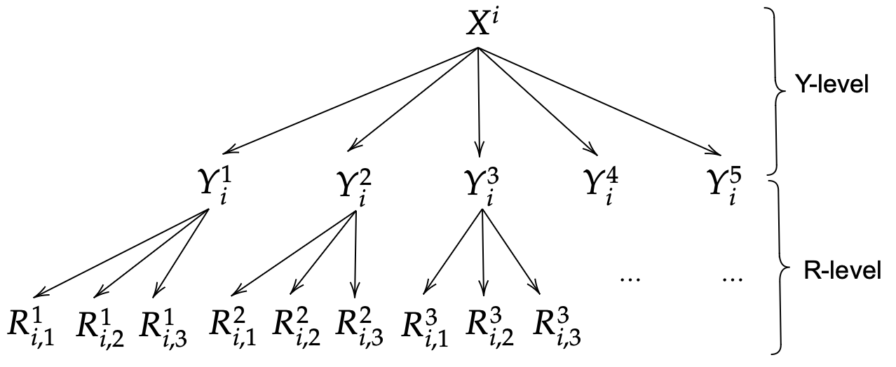
(a) Approach 1

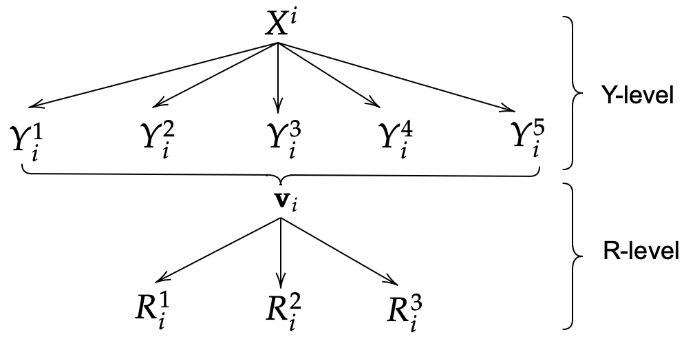
(b) Approach 2

Figure 2. Particle systems in tri-level optimization algorithm with $M=5$ particles for $Y$-system and $P=3$ particles for $R$-system. Y-level corresponds to the $Y$-particles solving the second level of optimization. In both approaches, they correspond to each fixed $X$-particle (here $X^{i}$). R-level corresponds to the $R$-particles solving the third level of optimization. In Approach 1, they correspond to each fixed $Y$-particle, whereas in Approach 2, they correspond to a representative (consensus) of the $Y$-particles.

However, in practice, this straightforward generalization is computationally expensive, since we need $N$ particles in $X$-system, $N\times M$ particles in $Y$-system and $N\times M\times P$ particles in $R$-system. Therefore, for tri-level optimization problems, we propose Approach 2 as illustrated in Figure 2. In the latter, we shall consider $N$ particles $\{X^{i}_{\cdot}\}_{i=1}^{N}$ in $\mathbb{R}^{n}$, and $M$ particles $(Y^{1}_{i,\cdot},\dots,Y^{M}_{i,\cdot})\in\left(\mathbb{R}^{m}\right)^{M}$ associated to each particle $X^{i}_{\cdot}$ as for bi-level problems. Then, we compute the consensus point $\mathbf{v}^{i}$ of $\{Y^{j}_{i,\cdot}\}_{j=1}^{M}$, for $1\leq i\leq N$, to which we associate a set of $P$ particles $\{R^{k}_{i,\cdot}\}_{k=1}^{P}\in\left(\mathbb{R}^{p}\right)^{P}$. The dynamics now only have $N$ particles in $X$-system, $N\times M$ particles in $Y$-system and $N\times P$ particles in $R$-system.

The pseudo-code corresponding to Approach 2 in Figure 2 is Algorithm 2, where the weight functions $\omega_{i}=\omega_{i}(x,y,r),i=1,2,3$, for some $\alpha_{1},\alpha_{2},\alpha_{3}>0$ are

$$\omega_{1}=\exp(-\alpha_{1}F(x,y,r)),\;\omega_{2}=\exp(-\alpha_{2}G(x,y,r)),\;\omega_{3}=\exp(-\alpha_{3}E(x,y,r)).$$

Similar to Algorithm 1 for bi-level problems, we can choose $M\ll N$, and $P\ll N$. Additionally, we set for simplicity $c=1$. We also introduce the notation $\mathbf{D}\equiv\mathbb{D}_{Q}^{\delta}$ and $\Psi\equiv\psi_{Q}$, which are the truncation functions defined in §3.1. Here, the truncation parameter (denoted therein by $R$) is now a fixed constant $Q>0$.

Recall $\mathbf{Y}_{i,t}=(Y^{1}_{i,t},\dots,Y^{M}_{i,t})$, and $\mathbf{R}_{i,t}=(R^{1}_{i,t},\dots,R^{P}_{i,t})$, for $1\leq i\leq N$ and $t\geq 0$.

Set parameters: $\gamma,\,\alpha_{1},\,\alpha_{2},\,\alpha_{3},\,\lambda,\,\sigma,\,\Delta t,\,T_{x},\,T_{y},\,T_{r},\,\delta$ ;

Initialize: $\mathbf{z}^{i}_{0}=X_{0}^{i}\sim\rho_{0},\;i=1,\ldots,N$; $Y^{j}_{i,0}\sim\mu_{0},\;j=1,\ldots,M$; $R^{k}_{i,0}\sim\gamma_{0},\;k=1,\ldots,P$; $t=0$, $\mathcal{T}_{x}=T_{x}/\Delta t$, $\mathcal{T}_{y}=T_{y}/\Delta t$, $\mathcal{T}_{r}=T_{r}/\Delta t$ ;

while $t\leq\mathcal{T}_{x}$ do

       for $i=1,\ldots,N$ do

             $\tau=0$ ;

             $\mathbf{v}_{\tau}^{i}=\sum\limits_{j=1}^{M}Y^{j}_{i,\tau}\frac{\omega_{2}(X_{t}^{i},Y^{j}_{i,\tau},\frac{1}{P}\sum_{k=1}^{P}R_{i,0}^{k})}{\sum\limits_{\ell=1}^{M}\omega_{2}(X_{t}^{i},Y^{\ell}_{i,\tau},\frac{1}{P}\sum_{k=1}^{P}R_{i,0}^{k})}$ ;

              /* Consensus of $\mathbf{Y}_{i,0}$ */

             $\mathbf{u}^{i}_{\tau}\leftarrow\mathbf{v}^{i}_{\tau}$ ;

             while  $\tau\leq\mathcal{T}_{y}$ do

                   $s=0$ ;

                   $\mathbf{r}^{i}_{s}\leftarrow\sum\limits_{k=1}^{P}R^{k}_{i,s}\frac{\omega_{3}(X_{t}^{i},\mathbf{v}^{i}_{\tau},R^{k}_{i,s})}{\sum\limits_{\ell=1}^{M}\omega_{3}(X^{i}_{t},\mathbf{v}^{M}_{i,\tau},R^{\ell}_{i,s})}$ ;

                    /* Consensus of $\mathbf{R}_{i,0}$ */

                   while  $s\leq\mathcal{T}_{r}$ do

                         $\mathbf{R}_{i,s}\leftarrow\mathbf{R}_{i,s}-\lambda\;\Psi\left(\mathbf{R}_{i,s}-\mathbf{r}^{i}_{s}\right)\Delta t+\sigma\mathbf{D}\left(\mathbf{R}_{i,s}-\mathbf{r}^{i}_{s}\right)W_{i,s}^{\mathbf{R}}$;

                         $\mathbf{r}^{i}_{s}\leftarrow\sum\limits_{k=1}^{P}R^{k}_{i,s}\frac{\omega_{3}(X_{t}^{i},\mathbf{v}^{i}_{\tau},R^{k}_{i,s})}{\sum\limits_{\ell=1}^{P}\omega_{3}(X^{i}_{t},\mathbf{v}^{i}_{\tau},R^{\ell}_{i,s})}$ ;

                          /* consensus of $\mathbf{R}_{i,s}$ */

                         $\mathbf{v}^{\prime}\leftarrow\sum\limits_{j=1}^{M}Y^{j}_{i,\tau}\frac{\omega_{2}(X^{i}_{t},Y^{j}_{i,\tau},\mathbf{r}_{s}^{i})}{\sum\limits_{\ell=1}^{M}\omega_{2}(X^{i}_{t},Y^{\ell}_{i,\tau},\mathbf{r}_{s}^{i})}$ ;

                         $\mathbf{v}^{i}_{\tau}\leftarrow(1-\gamma)\mathbf{v}^{i}_{\tau}+\gamma\mathbf{v}^{\prime}$ ;

                          /* FLA of $\mathbf{Y}_{i,\tau}$ */

                         $s\leftarrow s+1$;

                        

                   end while

                  $\mathbf{Y}_{i,\tau}\leftarrow\mathbf{Y}_{i,\tau}-\lambda\;\Psi\left(\mathbf{Y}_{i,\tau}-\mathbf{v}^{i}_{\tau}\right)\Delta t+\sigma\mathbf{D}\left(\mathbf{Y}_{i,\tau}-\mathbf{v}^{i}_{\tau}\right)W_{i,\tau}^{\mathbf{Y}}$ ;

                   $\mathbf{v}^{i}_{\tau}=\sum\limits_{j=1}^{M}Y^{j}_{i,\tau}\frac{\omega_{2}(X_{t}^{i},Y^{j}_{i,\tau},\mathbf{r}_{s}^{i})}{\sum\limits_{\ell=1}^{M}\omega_{2}(X_{t}^{i},Y^{\ell}_{i,\tau},\mathbf{r}_{s}^{i})}$ ;

                    /* Note that $s=\mathcal{T}_{r}$ */

                   $\mathbf{z}^{\prime}\leftarrow\sum\limits_{q=1}^{N}X^{q}_{t}\frac{\omega_{1}(X^{q}_{t},\mathbf{v}_{\tau}^{i},\mathbf{r}_{s}^{i})}{\sum\limits_{r=1}^{N}\omega_{1}(X_{t}^{r},\mathbf{v}_{\tau}^{i},\mathbf{r}_{s}^{i})}$ ;

                   $\mathbf{z}_{t}^{i}\leftarrow(1-\gamma)\mathbf{z}_{t}^{i}+\gamma\mathbf{z}^{\prime}$ ;

                    /* FLA of $X^{i}_{t}$; it depends on $i$ */

                   $\tau\leftarrow\tau+1$

             end while

            

       end for

      $\mathbf{X}^{i}_{t}\leftarrow\mathbf{X}^{i}_{t}-\lambda\Psi\left(\mathbf{X}^{i}_{t}-\mathbf{z}^{i}_{t}\right)\Delta t+\sigma\mathbf{D}\left(\mathbf{X}^{i}_{t}-\mathbf{z}_{t}^{i}\right)W^{\mathbf{X}}_{i,t}$ ;

       $t\leftarrow t+1$ ;

      

end while

$(\bar{X},\,\bar{\mathbf{v}},\,\bar{\mathbf{r}})\leftarrow\left(\frac{1}{N}\sum_{i=1}^{N}X_{\mathcal{T}_{x}}^{i},\;\frac{1}{N}\sum_{i=1}^{N}\mathbf{v}_{\mathcal{T}_{y}}^{i},\;\frac{1}{N}\sum_{i=1}^{N}\mathbf{r}_{\mathcal{T}_{r}}^{i}\right)$;

$X^{*}\leftarrow\sum\limits_{k=1}^{N}X_{\mathcal{T}_{x}}^{k}\frac{\omega_{1}(X_{\mathcal{T}_{x}}^{k},\bar{\mathbf{v}},\bar{\mathbf{r}})}{\sum\limits_{j=1}^{N}\omega_{1}(X_{\mathcal{T}_{x}}^{j},\bar{\mathbf{v}},\bar{\mathbf{r}})}$;

$Y^{*}\leftarrow\sum\limits_{k=1}^{N}\mathbf{v}_{\mathcal{T}_{y}}^{k}\frac{\omega_{2}(\bar{X},\mathbf{v}_{\mathcal{T}_{y}}^{k},\bar{\mathbf{r}})}{\sum\limits_{j=1}^{N}\omega_{2}(\bar{X},\mathbf{v}_{\mathcal{T}_{y}}^{j},\bar{\mathbf{r}})}$;

$R^{*}\leftarrow\sum\limits_{k=1}^{N}\mathbf{r}_{\mathcal{T}_{r}}^{k}\frac{\omega_{3}(\bar{X},\bar{\mathbf{v}},\mathbf{r}_{\mathcal{T}_{r}}^{k})}{\sum\limits_{j=1}^{N}\omega_{3}(\bar{X},\bar{\mathbf{v}},\mathbf{r}_{\mathcal{T}_{r}}^{j})}$;

Return $(X^{*},Y^{*},R^{*})$ ;

  /* Approximation of solution to (LABEL:trilevel_opt) */

Algorithm 2 multiscale CBO for tri-level optimization problem

5. Numerical experiments

In this section, we first assess the performance of the multiscale CBO algorithm for bi-level and tri-level optimization problems. Then, we compare the performance of multiscale CBO methods with the CBO methods proposed by [huang2024consensus] in solving min-max optimization problems. We shall construct multi-level optimization problems using the following benchmark functions:

1. Ackley function [Ackley]:

   (5.1) $$A(x):=-20\exp\left(-0.2\sqrt{\frac{1}{d}\sum_{i=1}^{d}x_{i}^{2}}\right)-\exp\left(\frac{1}{d}\sum_{i=1}^{d}\cos\left(2\pi x_{i}\right)\right)+\exp(1)+20.$$

2. Rastrigin function [rastrigin1974systems]:

   (5.2) $$R(x):=\sum_{i=1}^{d}x_{i}^{2}+1.5(1-\cos\left(2\pi x_{i}\right)).$$

3. Lévy function [levy1969utility]:

   (5.3) $$L(x):= \sin^{2}\left(\pi\left(1+\frac{x_{1}}{4}\right)\right)+\sum_{i=1}^{d-1}\left(\frac{x_{i}}{4}\right)^{2}\left[1+10\sin^{2}\left(\pi\left(1+\frac{x_{i}}{4}\right)+1\right)\right]$$

   $$\quad\quad\quad+\left(\frac{x_{d}}{4}\right)^{2}\left[1+\sin^{2}\left(2\pi\left(1+\frac{x_{i}}{4}\right)\right)\right],\qquad d\geq 2.$$

All the benchmarks have global minimizer $x^{*}=(0,\cdots,0)$. In the following, we perform 100 Monte Carlo simulations to compute the success rate of the multiscale CBO algorithm and expectation of the error, which is defined as

$$\texttt{error}:=\|X^{*}-x^{*}\|_{2}+\|Y^{*}-y^{*}\|_{2}$$

with output $(X^{*},Y^{*})$ for bi-level and min-max optimization algorithms, $(x^{*},y^{*})$ is the true solution. For tri-level optimization problem, given the output $(X^{*},Y^{*},R^{*})$ of Algorithm 2, the error is defined analogously as

$$\texttt{error}:=\|X^{*}-x^{*}\|_{2}+\|Y^{*}-y^{*}\|_{2}+\|R^{*}-r^{*}\|_{2},$$

where $(x^{*},y^{*},r^{*})$ is the true solution of the tri-level optimization problem. We consider a run is successful if

(5.4) $$\texttt{error}\leq 0.25,$$

following what has previously been done in [kalise2023consensus, pinnau2017consensus].

5.1. Bi-level optimization

In this section, we consider the bi-level optimization problem (1.1). The particle dynamics are discretized using the Euler–Maruyama scheme. The parameters are chosen as

(5.5) $$\alpha=\beta=10^{15},\quad T_{x}=50,\quad T_{y}=0.5,\quad\Delta t=\Delta\tau=0.1$$

$$N=100,\;M=25,\quad\lambda_{1}=\lambda_{2}=1,\quad\sigma_{1}=\sigma_{2}=2,\quad\gamma=0.75,$$

$$\delta_{1}=\delta_{2}=10^{-5},\quad R_{1}=R_{2}=10,\quad c=1,\quad n=m=d$$

The initial positions of $x$-particles and $y$-particles are sampled from $\rho_{0}=\mathcal{U}[-1,3]^{d}$ and $\mu_{0}=\mathcal{U}[-1,3]^{d}$, respectively. In Table 1 we display the numerical results obtained for bi-level optimization problems, MS-CBO refers to the multiscale CBO algorithm we propose, where MS stands for multiscale. The solutions for all the tests are at origin, except for the test (ii) whose solution is $x^{*}=y^{*}=(1,\cdots,1)$.

$d=10$		MS-CBO
(i)	$F(x,y)=\sum_{i=1}^{d}x_{i}^{2}+y_{i}^{2}$ $G(x,y)=\sum_{i=1}^{d}(x_{i}-y_{i})^{2}$	success rate	100%
		$\mathbb{E}[\texttt{error}]$	1.250$\times 10^{-4}$
		running time (s)	13.185
(ii)	$F(x,y)=\sum_{i=1}^{d}(x_{i}-1)^{2}+(y_{i}-1)^{2}$ $G(x,y)=\sum_{i=1}^{d}(x_{i}-y_{i})^{2}$	success rate	100%
		$\mathbb{E}[\texttt{error}]$	1.341$\times 10^{-4}$
		running time (s)	12.457
(iii)	$F(x,y)=\sum_{i=1}^{d}x_{i}^{2}+y_{i}^{2}+2x_{i}y_{i}$ $G(x,y)=\sum_{i=1}^{d}(x_{i}-y_{i})^{2}$	success rate	100%
		$\mathbb{E}[\texttt{error}]$	1.809$\times 10^{-3}$
		running time (s)	12.621
(iv)	$F(x,y)=A(x)+A(y)$ $G(x,y)=\sum_{i=1}^{d}(x_{i}-y_{i})^{2}$	success rate	100%
		$\mathbb{E}[\texttt{error}]$	1.415$\times 10^{-4}$
		running time (s)	13.739
(v)	$F(x,y)=R(x)+R(y)$ $G(x,y)=A(x-y)$	success rate	99%
		$\mathbb{E}[\texttt{error}]$	1.410$\times 10^{-2}$
		running time (s)	15.068
(vi)	$F(x,y)=L(x)+L(y)$ $G(x,y)=A(x-y)$	success rate	100%
		$\mathbb{E}[\texttt{error}]$	1.390$\times 10^{-4}$
		running time (s)	13.959

Table 1. The numerical results obtained with Algorithm 1 for bi-level optimization problems (1.1), where $n=m={\color[rgb]{0,0,1}d=10}$

We observe that Algorithm 1 demonstrates satisfactory accuracy in solving bi-level optimization problems, more importantly when the objective functions are non-convex with multiple local minimizers.

5.2. Tri-level optimization

In this section, we consider the tri-level optimization problem (LABEL:trilevel_opt) with $n=m=p=d$. The particles are sampled initially from $\rho_{0}=\mu_{0}=\gamma_{0}=\mathcal{U}[-1,3]^{d}$, and the parameters are chosen as

$$\alpha_{1}=\alpha_{2}=\alpha_{3}=10^{15},\;T_{x}=50,\;T_{y}=T_{z}=0.5,\;\Delta t=0.1,\;c=1$$

$$N=100,\;M=50,\;P=25,\;\lambda=1,\;\sigma=2,\;\gamma=0.75,\;\delta=10^{-5},\;Q=10.$$

The numerical results obtained for tri-level optimization problems are shown in Table 2. The optimal solution for Test (A) and Test (B) is $x^{*}=y^{*}=r^{*}=(0,\cdots,0)$ and the optimal solution for Test (C) is $x^{*}=y^{*}=r^{*}=(1,\cdots,1)$.

Test (A)
$F(x,y,r)=\sum_{i=1}^{d}x_{i}^{2}+y_{i}^{2}$ $G(x,y,r)=L(x-y)$ $E(x,y,r)=L(r-y)$	success rate	100%
	$\mathbb{E}[\texttt{error}]$	$1.603\times 10^{-3}$
	running time (s)	17.698
Test (B)
$F(x,y,r)=\sum_{i=1}^{d}x_{i}^{2}+y_{i}^{2}+(r_{i}-x_{i})^{2}$ $G(x,y,r)=L(x-y)$ $E(x,y,r)=R(r-y)$	success rate	95%
	$\mathbb{E}[\texttt{error}]$	$8.717\times 10^{-2}$
	running time (s)	14.588
Test (C)
$F(x,y,r)=\sum_{i=1}^{d}(x_{i}-1)^{2}+(y_{i}-1)^{2}+(r_{i}-1)^{2}$ $G(x,y,r)=\sum_{i=1}^{d}(y_{i}-x_{i})^{2}$ $E(x,y,r)=\sum_{i=1}^{d}(r_{i}-y_{i})^{2}$	success rate	100%
	$\mathbb{E}[\texttt{error}]$	$2.014\times 10^{-4}$
	running time (s)	15.117

Table 2. The numerical results obtained with Algorithm 2 for tri-level optimization problems (LABEL:trilevel_opt), where $n=m=p={\color[rgb]{0,0,1}d=10}$.

The results in Table 2 show that Algorithm 2 is capable of finding solutions to tri-level optimization problems and achieving satisfactory accuracy.

5.3. Min-max optimization

In this section, we consider the min-max optimization problem (1.3), where $F:\mathcal{X}\times\mathcal{Y}\rightarrow\mathbb{R}$, with $\mathcal{X}=\mathbb{R}^{d}$ and $\mathcal{Y}=\mathbb{R}^{d}$. We first consider the one dimensional setting to visualize the behaviour of the MS-CBO algorithm. The parameters are chosen as

$$\alpha=\beta=10^{15},\quad T_{x}=10,\;T_{y}=2,\quad\Delta t=\Delta\tau=0.1,\quad N=20,\;M=5,\quad c=1,$$

$$\lambda_{1}=\lambda_{2}=1,\quad\sigma_{1}=\sigma_{2}=1,\quad\gamma=0.75,\quad\delta_{1}=\delta_{2}=0.1,\quad R_{1}=R_{2}=10.$$

The $x$- and $y$-particles are sampled initially from $\rho_{0}=\mu_{0}=\mathcal{U}[-4,4]$. In the following figures, the blue points are the initial configuration $(X^{i}_{0},\mathbf{v}^{i}_{0})_{i=1}^{N}$, recall the definition of $\mathbf{v}^{i}_{t}$ in (2.9), and the red points are the final position of particles $(X^{i}_{\mathcal{T}_{x}},\mathbf{v}^{i}_{\mathcal{T}_{y}})_{i=1}^{N}$. The illustration are shown in Figure 3.

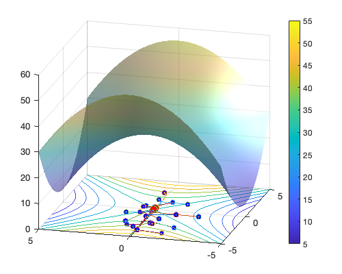
(a) Figure 1.1 $F(x,y)=x^{2}-y^{2}$

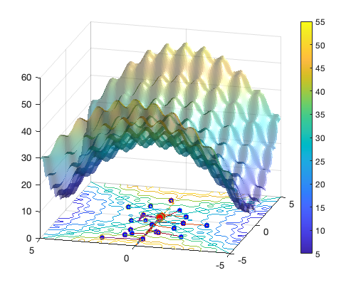
(b) Figure 1.2 $F(x,y)=R(x)-R(y)$

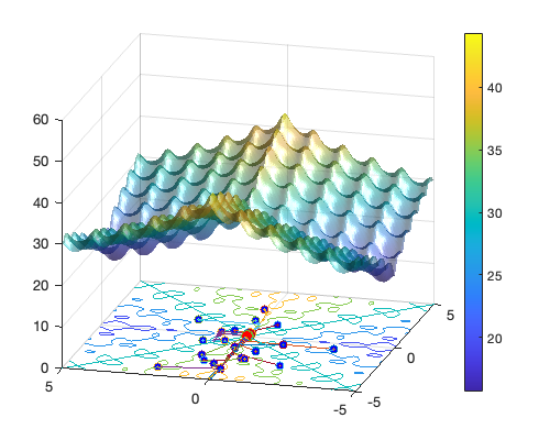
(c) Figure 1.3 $F(x,y)=A(x)-A(y)$

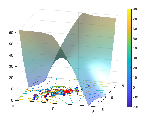
(d) Figure 1.4 $F(x,y)=x^{2}-y^{2}-2xy$

Figure 3. Illustration of the dynamics for multiscale CBO. The graph are shifted by $+30$ units.

Furthermore, we shall compare the performance of MS-CBO with the CBO algorithm proposed in [huang2024consensus] and which we shall hereafter refer to by SP-CBO, where SP stands for saddle points.

The test functions are defined as

1. Ackley function:

   $$F(x,y)=A(x)-A(y),$$

2. A non-separable (NS) Rastrigin function:

   $$F(x,y)=R(x)-R(y)-2\sum_{i=1}^{d}x_{i}y_{i},$$

3. Lévy function:

   $$F(x,y)=L(x)-L(y),$$

4. A non-separable function:

   $$F(x,y)=\sum_{i=1}^{d}x_{i}^{2}-\sum_{i=1}^{d}y_{i}^{2}-2\sum_{i=1}^{d}x_{i}y_{i}.$$

The parameters of both MS-CBO and SP-CBO are chosen as in (5.5).

Note that in SP-CBO, the number of particles in both the $X$- and $Y$-systems are $N$ and time horizon is chosen as $T=T_{x}=50$. The numerical experiments for the MS-CBO algorithm are divided into two cases: when $c=1$ and when $c=1/\sqrt{M}-0.01$. These results are collected in Table 3.

$d=10$		MS-CBO		SP-CBO
		$c=1$	$c=1/\sqrt{M}-0.01$
Function (a) Ackley	success rate	100%	100%	99%
	$\mathbb{E}[\texttt{error}]$	7.452$\times 10^{-5}$	1.412$\times 10^{-4}$	8.714$\times 10^{-3}$
	running time (s)	17.653	15.640	0.126
Function (b) NS-Rastrigin	success rate	97%	74%	5%
	$\mathbb{E}[\texttt{error}]$	5.123$\times 10^{-2}$	2.748 $\times 10^{-1}$	2.597
	running time (s)	18.387	16.438	0.136
Function (c) Lévy	success rate	100%	100%	99%
	$\mathbb{E}[\texttt{error}]$	8.694$\times 10^{-5}$	1.588$\times 10^{-4}$	2.664$\times 10^{-2}$
	running time (s)	16.491	15.972	0.156
Function (d) NS	success rate	100%	100%	100%
	$\mathbb{E}[\texttt{error}]$	1.585$\times 10^{-3}$	2.315$\times 10^{-3}$	1.474$\times 10^{-3}$
	running time (s)	18.307	14.855	0.037

Table 3. Numerical results for min-max optimization problems

All the results above were obtained using the random number generator rng in Matlab (R2021a) with seeds 1-100 for every 100 runs.

As mentioned in 3.3, we implement the for loop of $y$-particles in parallel with $T_{y}\ll T_{x}$. Although the running time of MS-CBO is larger than the running time of SP-CBO, the advantage is at the level of the numerical complexity, since we have $\mathcal{O}(N^{2})$ for SP-CBO, whereas MS-CBO is of $\mathcal{O}(NM)$ with $M\ll N$, in particular when choosing $M=\sqrt{N}$ one gets $\mathcal{O}(N^{3/2})$. This would be beneficial when the underlying dimension $d$ grows, or when the structure of the optimization problem becomes more complex (e.g. multi-level problems) for which a larger number of particles would be needed, and consequently a lower numerical complexity would be desirable. Numerical results for $M=\sqrt{N}$ are collected in Table 4.

One may increase the time horizon during which the algorithm runs, and hope to obtain better results. This strategy seems to be beneficial for SP-CBO in few cases only, for example when the objective function is quadratic with few local extrema. However, for more complicated objective functions such as (a),(b),(c), the accuracy of SP-CBO does not seem to improve simply by allowing for a longer running time. In such situation, MS-CBO turns out to be more advantageous, especially for nonconvex-nonconcave and non-separable functions with many local extrema, as is the case for example with function (b).

To further explore the performance of the algorithm MS-CBO, we now choose $M=\sqrt{N}$ while the other parameters are kept as in the previous test. The results we obtain in this setting are summarized in Table 4.

Function (b)		$N=200,\,M=14$	$N=400,\,M=20$	$N=600,\,M=25$
$d=8$	success rate	98%	100%	100%
	$\mathbb{E}[\texttt{error}]$	3.137 $\times 10^{-2}$	6.940$\times 10^{-4}$	8.847$\times 10^{-4}$
	running time (s)	20.206	22.089	34.271
$d=15$	success rate	2%	72%	100%
	$\mathbb{E}[\texttt{error}]$	1.618	3.067$\times 10^{-1}$	7.882$\times 10^{-3}$
	running time (s)	22.239	24.532	42.194
$d=20$	success rate	0%	13%	82%
	$\mathbb{E}[\texttt{error}]$	2.429	1.029	2.014$\times 10^{-1}$
	running time (s)	21.598	46.024	61.624

Table 4. The numerical results of MS-CBO in min-max optimization problems of Function (b) with $c=1$.

It can be seen from Table 4 that the accuracy of Algorithm 1 increases as the number of particles increases. With the choice of $M=\sqrt{N}$, MS-CBO is still able to find the solution to the min-max problem with (b) in relatively high-dimension.

6. Summary and conclusion

We have developed a multiscale version of the CBO algorithm, specifically designed for solving multi-level optimization problems. The main idea relies on a singularly perturbed system of SDEs: each scale corresponds to a level in the optimization problem. By using the celebrated averaging principle, this system is reduced to a single dynamics whose coefficients are averaged with respect to an invariant measure. The convergence of the original system to the averaged system has been proved in 3.1, and the presented algorithms have been tested on various optimization problems with satisfactory results.

Some practical modifications on the CBO model have been made in order to allow the averaging (obtained when $\varepsilon\to 0$) to be proved, in particular using a parameter $c$ to strengthen the drift term. In 3.1, this parameter is assumed to be small in order to guarantee the averaging. However, this is not a compulsory requirement in numerical implementation. Therefore, a sharper convergence analysis for broader choice of $c$ could be worth investigating. Another natural direction for further investigation is to explore the convergence guarantees of mean-field dynamics to the global solution of the optimization problem. We can study the mean-field limit of the averaged (effective) model (3.2) as $N\rightarrow\infty$, similar to the theoretical analysis of standard CBO methods. Yet, this is a challenging topic as difficulty arises from the invariant measure and its regularity with respect to the $x$-variable. On the other hand, the criteria of choosing optimal parameters in different dynamics remain to be understood, e.g., a more precise relationship is to be established between $M$ and $N$, $T_{x}$ and $T_{y}$ in bi-level problems. Lastly, in both Algorithms 1 and 2, we used the approximation (FLA) to handle the averaging with respect to the invariant measure. But we believe the implementation of the two algorithms could be further improved if one improves the computation of the invariant measure or the averaging with its respect.

Appendix A Proof of Theorem 3.1

We start by defining some functional spaces that we shall use.

• If $\theta\in(0,1)$, then $C^{\theta}_{b}(\mathbb{R}^{d})$ denotes the usual space of locally Hölder continuous functions with exponent $\theta$, and that are moreover bounded.

• If $\theta=1$, then $C^{1}_{b}(\mathbb{R}^{d})$ denotes the space of bounded and Lipschitz continuous functions.

• If $\theta\in(1,2)$, then $C^{\theta}_{b}(\mathbb{R}^{d})$ denotes the space of functions that are in $C^{1}_{b}(\mathbb{R}^{d})$ and whose first-order derivatives are in $C^{\theta-1}_{b}(\mathbb{R}^{d})$, noting that $\theta-1\in(0,1)$.

• If $\theta=2$, then $C^{2}_{b}(\mathbb{R}^{d})$ denotes the space of bounded functions whose first-order derivatives are Lipschitz continuous.

Now let $(x,y)\in\mathbb{R}^{d_{1}}\times\mathbb{R}^{d_{2}}$ for some $d_{1},d_{2}\in\mathbb{N}$, and let $f=f(x,y)$ be a function of $(x,y)$. We denote by $C_{b}^{\theta,\delta}:=C_{b}^{\theta}(\mathbb{R}^{d_{1}};C_{b}^{\delta}(\mathbb{R}^{d_{2}}))$ the space functions $f$ such that $x\mapsto f(x,y)\in C_{b}^{\theta}(\mathbb{R}^{d_{1}})$ locally uniformly in $y$, and $y\mapsto f(x,y)\in C_{b}^{\delta}(\mathbb{R}^{d_{2}})$ locally uniformly in $x$.

Proof of Theorem 3.1.

This shall be a consequence of statement $(i)$ in [rockner2021diffusion, Theorem 2.3] or, more precisely, of the particular case discussed in statement $(i)$ of Remark 2.5 therein. (A similar result can also be found in [rockner2019strong, Theorem 2.5].)
Therefore, it suffices to check that our system of coupled SDEs (3.1) satisfies the assumptions in [rockner2021diffusion]. To this end, and for better readability, we first highlight the correspondence between our notation and the one in [rockner2021diffusion] as follows:

$$\text{\textbullet\; in \cite[cite]{[\@@bibref{}{rockner2021diffusion}{}{}]}}: X^{\varepsilon}, Y^{\varepsilon},\; b, \sigma,\; F, G,\; c, H,\; \alpha_{\varepsilon}.$$

$$\text{\textbullet\; in \eqref{ms_CBO}}: \mathds{Y}\,, \mathds{X},\; \mathscr{B}, \mathscr{H},\; \mathscr{F}, \mathscr{G},\; 0, \,0,\; \sqrt{\varepsilon}.$$

We can now state the assumptions needed, and prove that they are satisfied.

1. $\mathscr{H}\mathscr{H}^{*}$ is bounded and non-degenerate in $y$, uniformly with respect to $x$. (This corresponds to assumptions $(A_{\sigma})$ in [rockner2021diffusion].)

2. $\mathscr{G}\mathscr{G}^{*}$ is bounded and non-degenerate in $x$, uniformly with respect to $y$. (This corresponds to assumptions $(A_{G})$ in [rockner2021diffusion].)

3. The drift of the fast process satisfies a recurrence assumption which ensures the existence of an invariant measure $\Upsilon_{x}(\text{d}y)$, and that is

   $$\lim\limits_{|y|\to+\infty}\,\sup\limits_{x}\,\langle y,\,\mathscr{B}(x,y)\rangle=-\infty.$$

   (This corresponds to assumptions $(A_{b})$ in [rockner2021diffusion].)

4. The coefficients $\mathscr{F},\mathscr{G}$ (of the slow variables $\mathds{X}$), and $\mathscr{B},\mathscr{H}$ (of the fast variables $\mathds{Y}$) are in $C_{b}^{\theta,\delta}$, with $\theta\in(0,1)$ and $\delta\in(0,1)$. (This is an assumption slightly stronger than the regularity requirement in [rockner2021diffusion].)

Our construction of $\mathscr{H}$ and $\mathscr{G}$ in §2.3 guarantee the validity of assumptions (i) and (ii). To check assumption (iii), we proceed as follows. Given $\mathbf{x}=(x_{i})_{1\leq i\leq N}$, where $x_{i}\in\mathbb{R}^{n}$, and setting

$$\mathds{Y}=(\mathbf{Y}_{i})_{1\leq i\leq N}\in\mathbb{R}^{mMN},\quad\text{ where }\mathbf{Y}_{i}=(Y^{j}_{i})_{1\leq j\leq M}\in\mathbb{R}^{mM},\quad\text{ and }Y^{j}_{i}\in\mathbb{R}^{m},$$

with $Y^{j}_{i}=(Y^{j}_{i}(k))_{1\leq k\leq m}$, we have

$$\mathscr{B}(\mathbf{x},\mathds{Y})=\big{(}B(x_{i},\mathbf{Y}_{i})\big{)}_{1\leq i\leq N},\quad\text{ where }\quad B(x_{i},\mathbf{Y}_{i})=\big{(}b_{i}^{j}(x_{i},\mathbf{Y}_{i})\big{)}_{1\leq j\leq M}$$

and

$$b_{i}^{j}(x_{i},\mathbf{Y}_{i}) =-\lambda_{2}\,\psi_{R_{2}}\left(\,Y_{i}^{j}-c\,\sum_{k=1}^{M}Y_{i}^{k}\frac{\varpi_{\beta}\left(x_{i},Y_{i}^{k}\right)}{\sum_{\ell=1}^{M}\varpi_{\beta}\left(x_{i},Y_{i}^{\ell}\right)}\,\right)\in\mathbb{R}^{m}$$

using the truncation function defined, for a vector $v\in\mathbb{R}^{d}$, by

$$\psi_{R}(v)=\big{(}\psi_{R}(v)_{k}\big{)}_{1\leq k\leq d}\quad\text{ where }\psi_{R}(v)_{k}=\left\{\;\begin{aligned} &v_{k}\;,\quad\quad\text{ if }\;|v_{k}|\leq R\\ &\frac{v_{k}}{|v_{k}|}R\;,\quad\text{ if }\;|v_{k}|>R.\end{aligned}\right.$$

Then we obtain

(A.1) $$\langle\,\mathds{Y},\,\mathscr{B}(x,\mathds{Y})\,\rangle=\sum\limits_{i=1}^{N}\;\langle\,\mathbf{Y}_{i},\,B(x_{i},\,\mathbf{Y}_{i})\,\rangle=\sum\limits_{i=1}^{N}\sum\limits_{j=1}^{M}\;\langle\,Y_{i}^{j},\,b_{i}^{j}(x_{i},\mathbf{Y}_{i})\,\rangle$$

and

$$\langle\,Y_{i}^{j},\,b_{i}^{j}(x_{i},\mathbf{Y}_{i})\,\rangle =-\lambda_{2}\,\langle\,Y_{i}^{j},\,\psi_{R_{2}}\left(\,Y_{i}^{j}-c\,\sum_{k=1}^{M}Y_{i}^{k}\frac{\varpi_{\beta}\left(x_{i},Y_{i}^{k}\right)}{\sum_{\ell=1}^{M}\varpi_{\beta}\left(x_{i},Y_{i}^{\ell}\right)}\,\right)\,\rangle.$$

Notice that, for any $w,v\in\mathbb{R}^{d}$, we have $\langle w,\psi_{R_{2}}(v)\rangle=\sum_{\tau=1}^{d}\langle w,\psi_{R_{2}}(v)\rangle_{\tau}$ and

$$\langle w,\psi_{R_{2}}(v)\rangle_{\tau}=\left\{\;\begin{aligned} &w_{\tau}v_{\tau}\;,\quad\quad\text{ if }\;|v_{\tau}|\leq R_{2},\\ &w_{\tau}v_{\tau}\frac{R}{|v_{\tau}|}\;,\quad\text{ if }\;|v_{\tau}|>R_{2},\end{aligned}\right.\quad\tau=1,\dots,d.$$

We can then write $\langle w,\psi_{R_{2}}(v)\rangle_{\tau}=w_{\tau}v_{\tau}\,\xi(v_{\tau})$ where $\xi(v_{\tau}):=1\wedge\frac{R_{2}}{|v_{\tau}|}$, and $\xi(0)=1$. Note in particular that $0<\xi(v_{\tau})\leq 1$ for all $v_{\tau}\in\mathbb{R}$. Therefore we have, for $\tau=1,\dots,m$

$$\langle\,Y_{i}^{j},\,b_{i}^{j}(x_{i},\mathbf{Y}_{i})\,\rangle_{\tau}$$

$$\quad\quad=\bigg{(}-\lambda_{2}\,Y_{i}^{j}(\tau)^{2}+\lambda_{2}\,c\;\sum_{k=1}^{M}Y_{i}^{j}(\tau)Y_{i}^{k}(\tau)\frac{\varpi_{\beta}\left(x_{i},Y_{i}^{k}\right)}{\sum_{\ell=1}^{M}\varpi_{\beta}\left(x_{i},Y_{i}^{\ell}\right)}\,\bigg{)}$$

$$\quad\quad\quad\quad\quad\quad\quad\quad\quad\times\xi\bigg{(}\,Y_{i}^{j}(\tau)-c\,\sum_{k=1}^{M}Y_{i}^{k}(\tau)\frac{\varpi_{\beta}\left(x_{i},Y_{i}^{k}\right)}{\sum_{\ell=1}^{M}\varpi_{\beta}\left(x_{i},Y_{i}^{\ell}\right)}\,\bigg{)}.$$

Let us denote by $\underline{\xi}$ the following

$$\underline{\xi}(\mathds{Y}):=\min\limits_{\begin{subarray}{c}1\leq\tau\leq m\\ 1\leq j\leq M\\ 1\leq i\leq N\end{subarray}}\left\{\xi\bigg{(}\,Y_{i}^{j}(\tau)-c\,\sum_{k=1}^{M}Y_{i}^{k}(\tau)\frac{\varpi_{\beta}\left(x_{i},Y_{i}^{k}\right)}{\sum_{\ell=1}^{M}\varpi_{\beta}\left(x_{i},Y_{i}^{\ell}\right)}\,\bigg{)}\right\}\,\in(0,1].$$

We have

(A.2) $$\langle\,Y_{i}^{j},\,b_{i}^{j}(x_{i},\mathbf{Y}_{i})\,\rangle_{\tau} \leq-\lambda_{2}\,Y_{i}^{j}(\tau)^{2}\,\underline{\xi}(\mathds{Y})+\lambda_{2}\,c\,\Theta_{i}^{j}(\tau)$$

where

$$\Theta_{i}^{j}(\tau) :=\bigg{(}\sum_{k=1}^{M}Y_{i}^{j}(\tau)Y_{i}^{k}(\tau)\frac{\varpi_{\beta}\left(x_{i},Y_{i}^{k}\right)}{\sum_{\ell=1}^{M}\varpi_{\beta}\left(x_{i},Y_{i}^{\ell}\right)}\,\bigg{)}$$

$$\quad\quad\quad\times\,\xi\bigg{(}\,Y_{i}^{j}(\tau)-c\,\sum_{k=1}^{M}Y_{i}^{k}(\tau)\frac{\varpi_{\beta}\left(x_{i},Y_{i}^{k}\right)}{\sum_{\ell=1}^{M}\varpi_{\beta}\left(x_{i},Y_{i}^{\ell}\right)}\,\bigg{)}.$$

Taking the absolute value, and using $|\xi(\cdot)|\leq 1$, one gets

$$\big{|}\Theta_{i}^{j}(\tau)\big{|} \leq\sum_{k=1}^{M}|Y_{i}^{j}(\tau)|\,|Y_{i}^{k}(\tau)|\,\frac{\varpi_{\beta}\left(x_{i},Y_{i}^{k}\right)}{\sum_{\ell=1}^{M}\varpi_{\beta}\left(x_{i},Y_{i}^{\ell}\right)},$$

and then

$$\sum\limits_{\tau=1}^{m}\big{|}\Theta_{i}^{j}(\tau)\big{|} \leq\sum_{k=1}^{M}\sum\limits_{\tau=1}^{m}|Y_{i}^{j}(\tau)|\,|Y_{i}^{k}(\tau)|\,\frac{\varpi_{\beta}\left(x_{i},Y_{i}^{k}\right)}{\sum_{\ell=1}^{M}\varpi_{\beta}\left(x_{i},Y_{i}^{\ell}\right)}.$$

Using Cauchy–Schwarz inequality yields

$$\sum\limits_{\tau=1}^{m}\big{|}\Theta_{i}^{j}(\tau)\big{|} \leq\sum_{k=1}^{M}\left(\sum\limits_{\tau=1}^{m}|Y_{i}^{j}(\tau)|^{2}\right)^{\frac{1}{2}}\left(\sum\limits_{\tau=1}^{m}|Y_{i}^{k}(\tau)|^{2}\right)^{\frac{1}{2}}\frac{\varpi_{\beta}\left(x_{i},Y_{i}^{k}\right)}{\sum_{\ell=1}^{M}\varpi_{\beta}\left(x_{i},Y_{i}^{\ell}\right)}$$

$$=\sum_{k=1}^{M}\|Y_{i}^{j}\|\,\|Y_{i}^{k}\|\,\frac{\varpi_{\beta}\left(x_{i},Y_{i}^{k}\right)}{\sum_{\ell=1}^{M}\varpi_{\beta}\left(x_{i},Y_{i}^{\ell}\right)}$$

$$\leq\left(\sum_{k=1}^{M}\|Y_{i}^{j}\|^{2}\,\frac{\varpi_{\beta}\left(x_{i},Y_{i}^{k}\right)}{\sum_{\ell=1}^{M}\varpi_{\beta}\left(x_{i},Y_{i}^{\ell}\right)}\right)^{\frac{1}{2}}\left(\sum_{k=1}^{M}\|Y_{i}^{k}\|^{2}\,\frac{\varpi_{\beta}\left(x_{i},Y_{i}^{k}\right)}{\sum_{\ell=1}^{M}\varpi_{\beta}\left(x_{i},Y_{i}^{\ell}\right)}\right)^{\frac{1}{2}}$$

$$=\|Y_{i}^{j}\|\left(\sum_{k=1}^{M}\|Y_{i}^{k}\|^{2}\,\frac{\varpi_{\beta}\left(x_{i},Y_{i}^{k}\right)}{\sum_{\ell=1}^{M}\varpi_{\beta}\left(x_{i},Y_{i}^{\ell}\right)}\right)^{\frac{1}{2}}$$

$$\leq\|Y_{i}^{j}\|\left(\sum_{k=1}^{M}\|Y_{i}^{k}\|^{2}\right)^{\frac{1}{2}}=\|Y_{i}^{j}\|\,\|\mathbf{Y}_{i}\|.$$

The latter inequality together with (A.2) yield

$$\langle\,Y_{i}^{j},\,b_{i}^{j}(x_{i},\mathbf{Y}_{i})\,\rangle =\sum\limits_{\tau=1}^{m}\langle\,Y_{i}^{j},\,b_{i}^{j}(x_{i},\mathbf{Y}_{i})\,\rangle_{\tau}$$

$$\leq-\lambda_{2}\,\underline{\xi}(\mathds{Y})\,\|Y_{i}^{j}\|^{2}+\lambda_{2}\,c\,\|Y_{i}^{j}\|\,\|\mathbf{Y}_{i}\|,$$

and with (A.1), one obtains (using again Cauchy-Schwarz inequality)

$$\langle\,\mathds{Y},\,\mathscr{B}(x,\mathds{Y})\,\rangle =\sum\limits_{i=1}^{N}\sum\limits_{j=1}^{M}\;\langle\,Y_{i}^{j},\,b_{i}^{j}(x_{i},\mathbf{Y}_{i})\,\rangle$$

$$\leq-\lambda_{2}\,\underline{\xi}(\mathds{Y})\,\|\mathds{Y}\|^{2}+\lambda_{2}\,c\,\sum\limits_{i=1}^{N}\sum\limits_{j=1}^{M}\|Y_{i}^{j}\|\,\|\mathbf{Y}_{i}\|$$

$$\leq-\lambda_{2}\,\underline{\xi}(\mathds{Y})\,\|\mathds{Y}\|^{2}+\lambda_{2}\,c\,\sum\limits_{i=1}^{N}\big{(}\|\mathbf{Y}_{i}\|\big{)}\,\big{(}\sqrt{M}\,\|\mathbf{Y}_{i}\|\big{)}$$

$$=-\lambda_{2}\,\underline{\xi}(\mathds{Y})\,\|\mathds{Y}\|^{2}+\lambda_{2}\,c\,\sqrt{M}\,\|\mathds{Y}\|^{2}=-\lambda_{2}\big{(}\underline{\xi}(\mathds{Y})-c\sqrt{M}\big{)}\|\mathds{Y}\|^{2}.$$

Therefore, in order to satisfy assumption (iii), it suffices to have

$$c<\frac{\underline{\xi}(\mathds{Y})}{\sqrt{M}}.$$

Let us note that $\underline{\xi}(\mathds{Y})$ tends to $1$ when the particles $Y_{i}^{j}$ tends to a consensus, and $\underline{\xi}(\mathds{Y})$ tends to $0$ only when a $Y_{i}^{j}$ gets (infinitely) far from the others, the latter being a behavior that is not likely to happen, provided we choose the radius $R_{2}$ of the truncation large enough compared to the closed ball containing the initial position of the particles. This will prevent $\xi(\mathds{Y})$ from getting smaller, allowing $c$ to exist.

Finally, the coefficients in (3.1) are bounded and locally Hölder continuous with any exponent in $(0,1)$, hence the validity of assumption (iv).

Thus we can apply the result in [rockner2021diffusion] with coefficients that are bounded in both $x,y$, and locally Hölder continuous with exponents $\theta,\delta\in(0,1)$, which concludes the proof. ∎