Predicting properties of quantum systems by regression on a quantum computer
Abstract
Quantum computers can be considered as a natural means for performing machine learning tasks for labeled data which are inherently quantum. Many quantum machine learning techniques have been developed for solving classification problems, such as distinguishing between phases of matter or quantum processes. Similarly, one can consider a more general problem of regression, when the task is to predict continuous labels quantifying some property of quantum states, such as purity or entanglement. In this work, we propose a data-agnostic method for predicting such properties. The method is based on the notion of parametrized quantum circuits, and it seeks to find an observable the expectation of which gives the estimation of the property of interest with presumably low variance. We numerically test our approach in learning to predict (i) the parameter of a parametrized channel given its output state, (ii) entanglement of two-qubit states, and (iii) the parameter of a parametrized Hamiltonian given its ground state. The results show that the proposed method is able to find observables such that they provide highly accurate predictions of the considered properties, and in some cases even saturate the Cramer-Rao bound, which characterizes the prediction error.
I Introduction
Quantum machine learning (QML) is a promising application for quantum computers [1, 2, 3, 4, 5]. In QML, one commonly considers datasets of labeled classical data points mapped to quantum states via various encoding strategies [6, 7, 8, 9]. Very often data labeled with discrete labels need to be classified [10, 11, 12], or a regression problem has to be solved for predicting continuous labels [13, 14, 15, 16].
One approach for solving these problems uses kernel-based methods centered around computing a similarity measure (inner products) between data points [17, 18, 19]. The other approach of processing quantum states in QML is built upon the notion of parametrized (sometimes called variational) quantum circuits [20, 21]. These circuits essentially are parametrized unitary operators used for transforming quantum states, depending on the task [22, 23]. For instance, one can find the ground state of a given Hamiltonian [24, 25, 26], solve linear algebra problems [27, 28], perform state [29] and Hamiltonian diagonalization [30, 31, 32], etc. Additionally, variational quantum computing methods have been applied for quantum metrology and parameter estimation [33, 34, 35], i.e. for finding optimal input states and measurements which provide an estimation of the parameter(s) of a quantum channel as precise as possible [36, 37, 38].
QML techniques can also be used for processing data which are initially quantum. One can, for instance, classify phases of matter [39, 40, 41], detect anomalies in sets of quantum states [42, 43], and discern between quantum states [44, 45] and quantum channels [46, 47, 48]. Additionally, one can apply QML for simulating the dynamics of quantum systems [49], detecting and classifying entanglement in quantum states [50, 51], and even discovering quantum algorithms [52] as well as error correction codes [53].
In this work, we propose a method for solving regression tasks for labeled data represented by quantum states with labels . The method is based on variational quantum circuits, and is agnostic to the connection between the labeled states and their labels. Among such connections, we consider: (i) the labeled state is an output state of a parametrized channel for some fixed input , (ii) is an entanglement measure of , and (iii) is such that is the ground state of a parametrized Hamiltonian . Case (i) is often considered in quantum metrology and channel estimation, (ii) is similar to the problem of entanglement quantification [54, 55], and (iii) can be viewed as a generalization of the classification of phases of matter [16].
The performance of our method is assessed with quantum Fisher information, a key concept of quantum metrology [56, 57]. Using that notion, one can lower-bound the error of the prediction of the label, and so we compare the results given by our method with this bound.
This work is structured as follows. In Section II we formulate the problem setting, describe the method of predicting the labels of labeled states, and introduce the Fisher information and Cramer-Rao bounds. Section III shows the results of the numerical application of the method for predicting the entanglement of the Bell-type and isotropic states, as well as two-qubit random pure and mixed states. The work is concluded with Section IV where we discuss the results and outline directions for further studies.
II Methods
We start with establishing the notation and the formulation of the regression problem. For this problem, we present a method for estimating the label of a given datum. Then we discuss the importance of the variance of this estimation, introduce both classical and quantum Fisher information, and use the latter to bound the estimation error.
II.1 Problem statement
Suppose we are given the following training set:
| (1) |
where are labeled data points and are their corresponding labels. We consider the data points to be quantum states described by density operators, i.e. and . Hereinafter, we assume that describes a state of qubits, so that acts in a Hilbert space of dimensionality . Given the training set the goal is to learn the estimation of parameters for unseen data (the data not present in ).
Essentially, we formulate a regression problem with data points being represented by quantum states. It should be emphasized that we assume no knowledge about the connection of the states with their labels . One instance of such connection is quantifying the entanglement of the state . Thus, our aim is to devise a method for predicting the labels to be as data-agnostic as possible.
II.2 The estimator and the cost function
We construct an estimator for as
| (2) |
where and the operators form a positive operator-valued measure (POVM),
where is the identity operator. For a given state , our estimate is essentially the expected value of an observable represented by a POVM with the corresponding measurement outcomes measured with respect to . To find optimal and , we minimize the least squares between the labels given in and our estimations ,
| (3) |
In other words, the operators with the corresponding outcomes form an engineered observable. If this observable is measured with respect to a state , it gives an estimation as close to a given as possible.
It is not difficult to optimize over a set of real numbers . However, the problem is more challenging for . Nonetheless, the POVM elements can be found with the variational quantum computing approach. Let us assume that , i.e., the operators in are orthogonal projectors. With this assumption, we can obtain POVM elements as
| (4) |
where is the projector onto the th state of the computational basis, and is a variational ansatz, i.e., a quantum circuit parametrized by . That is, instead of optimizing over the operators , we optimize over real numbers . Denoting , we rewrite (3) as
| (5) |
Note that in the case of an orthogonal POVM (4), one can associate the measurement operators and the corresponding measurement outcomes with an -qubit Hermitian operator , which has and as its eigenvalues and eigenprojectors, respectively,
| (6) |
Omitting the dependence on and , we can rewrite the estimator (2) simply as , i.e., the expected value of in the state . Equivalently, we can say that we transform the state with a unitary , measure the resulting state in the computational basis , and associate the outcome with the eigenvalue . Note also that if the ansatz is expressive enough, there is always an assignment for and such that the decomposition (6) gives any Hermitian matrix of the size .
In order to obtain a non-orthogonal POVM, one can utilize the Naimark’s extension theorem. Namely, one can attach an auxiliary quantum system in a pure state, say, , and find a variational ansatz acting on the joint state such that [58, 12]
| (7) |
Thus, one can measure a non-orthogonal POVM by measuring an orthogonal POVM in an extended Hilbert space. The dimensionality of this extension should coincide with the number of the POVM elements.
II.3 Number of measured qubits
It was assumed above that we measure all qubits of the -qubit state making the number of varied parameters exponentially large. In some cases, however, it may be sufficient to measure only out of qubits. Hence, we can modify the observable (6) to
| (8) |
for which one can take the POVM elements to be, e.g.,
| (9) |
Schematically, the process of measuring such with respect to can be depicted as follows:
That is, we measure the last qubits of the state in the computational basis, and with probability get the outcome associated with , evaluating the expectation therefore to .
In the case of measuring all qubits, the parametrized unitary can be, e.g., a hardware-efficient ansatz [25]. If we measure only or 2 qubits, the circuit may take the form of a quantum convolutional neural network (QCNN) [59]. In Appendix A, we show examples of both such ansätze. Alongside with having fixed depth and being resistant to the phenomenon of vanishing gradients [60], QCNNs in our setting also allow to decrease the number of varied parameters to . However, as we show in this work, for achieving better results for some tasks one needs to measure all qubits of the -qubit states; we discuss one of such cases in Appendix B.1.
II.4 Estimation variance
One can estimate the label of a given as the expected value of an observable measured with respect to the state , i.e., . Let us now consider the variance of such estimation.
As a simple example, assume that is an output state of a single-qubit depolarizing channel acting on an input state :
| (10) |
where the parameter can take values from to [61]. Let us also assume that the input state is , where is a Pauli operator and . Now, consider a single-qubit Hermitian observable decomposed in the Pauli basis:
where is the single-qubit identity. One can show that , , and arbitrary and give the expectation . At the same time, the variance of in the state is
| (11) | ||||
| (12) |
Thus, even if an observable produces a target expectation, the variance could be substantial. This is crucial since the variance is connected to the mean squared error (MSE) of the estimation via the error propagation formula [62, 63, 64, 65]
| (13) |
where we have used the shorthand and is the number of measurements.
Obviously, the variance should be included in our label prediction approach. We first rewrite the expressions (2) and (11). Let us denote the probability of obtaining the outcome after measuring in the state as . Since has the form (6) we get
| (14) |
Similarly, for the variance we obtain
| (15) |
It is important that both the expectation (14) and the variance (15) can be calculated from the same measurement results. Indeed, experimentally, one obtains only the probabilities as frequencies with being the number of times the outcome was observed, and the total number of measurements. Therefore, with little post-processing overhead we modify the optimization procedure (5) such that it takes into account the variance of our observable,
| (16) |
where
| (17) | |||
| (18) |
with being the weights. We seek to simultaneously minimize the least squares between the given labels and expectations in (17), and the variance of the observable in (18). In Appendix B.4.1, we show how by adjusting the weights and one can trade-off between a higher estimation accuracy and a lower variance.
II.5 Fisher information
The MSE is known to be lower-bounded by the classical Cramer-Rao bound (cCRB) [63]:
| (19) |
where is the classical Fisher information (cFI) which in our setup can be written as [34]
| (20) |
with depending on through .
Classical Fisher information is known to be upper-bounded by its quantum counterpart . To obtain the latter one introduces the symmetric logarithmic derivative (SLD) operator ,
| (21) |
and calculates the quantum Fisher information (qFI) as
| (22) |
In Appendix C we list various ways of finding and computing .
With qFI, one can obtain a tighter version of the bound (19) called the quantum Cramer-Rao bound (qCRB), namely,
| (23) |
Thus, cFI , being dependent on both the measurements and state , is upper bounded by qFI , which depends solely on the state . One can find the measurement operators such that cFI attains its maximum [56],
In order to find such optimal measurements one could compute the eigenprojectors of the SLD operator introduced in (55) [63]. Additionally, one can use itself for constructing an optimal observable
| (24) |
resulting in
However, the eigenprojectors of (i.e. also the optimal measurements ) generally depend on the parameter to be estimated. Therefore, it is often impossible to find a POVM such that it saturates qCRB over the entire range of . We will treat the Cramer-Rao bounds (23) as a figure of merit for our method for predicting the label for a given .
II.6 Biased estimator
We constructed above our estimation of for a given to be the expected value of an observable measured in the state . In general, however, such expectation could also contain a bias , i.e. [63]
with the estimation obtained from a measurement with the MSE [62]. In this biased case the earlier expressions have to be adjusted. Indeed, if , instead of the MSE , one would rather observe in an experiment. We can transform the corresponding formulas (13) and (19) to [66]
| (25) | |||
| (26) |
See Appendix D for a detailed derivation.
The bias of estimation could be worked around by inversion of the function [67]. Indeed, if is bijective within a range of , then one gets the desired estimation as . Alternatively, one could try to compensate the bias , as one extracts it from the difference between the estimation and the true labels given in the training set (see Appendix B.4.2).
Another strategy of sorting out an unwanted bias is modifying the estimator itself to be
| (27) |
i.e. we process copies of the -qubit state simultaneously, and is now a -qubit observable. This introduces a non-linearity to the estimation [68, 69]. Similar techniques are utilized in QML to improve its performance [21, 9, 12, 19]. In Appendix B.5.3 we apply this method to a problem of estimating for , in which case one cannot find giving the expectation . However, we show that for any there is an observable such that the expectation gives the first terms of the Fourier series of .
III Results
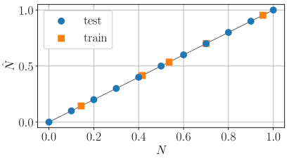
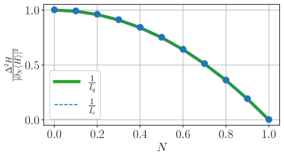
In this Section, we present the results of numerical experiments of the regression problem solution for the data of the form (1) with our method, i.e. we solve the optimization problem (16), minimizing the least squares (17) between the true parameters and our estimations as well as the variance of the observable (18) simultaneously.
As a test example we focus on entanglement quantification [70, 71, 72, 73, 54, 55]. The model is trained to predict the negativity of a given two-qubit state ,111We dropped an additional factor which often appears in the literature. All related expressions have been modified accordingly
| (28) |
where is the trace norm, and is the partial transpose of with respect to the second qubit. For more details on the negativity and bipartite entanglement overall, see Appendix E. Additionally, in Appendix B we show the results of applying our method to predict the parameter of a channel given its output state , and the parameter of a Hamiltonian given its ground state .
Where applicable, the classical and quantum Fisher informations were calculated using formulas (20) and (59), respectively. If not stated otherwise, we use a two-layered hardware-efficient ansatz described in Appendix A to represent the parametrized unitary , and set and . For optimization the BFGS algorithm is applied. Additionally, we use tools from the QuTiP package [74, 75].
III.1 Bell-type states
First, we train the model (16) to predict the negativity (28) of Bell-type states of the form
| (29) |
The training set is , where the coefficients are picked randomly from a uniform distribution. The observable is composed in the form (8) and only qubit of a two-qubit state (29) is measured.
Fig. 1 shows the performance of the trained model on the set with equidistant negativities . As can be seen, not only the accurate predictions of the negativity are obtained, but also the optimized observable saturates qCRB (23).
The explanation for such good performance could be the following. The negativity of the state (29) reads . Then one gets . Therefore, (29) can be rewritten as
| (30) |
where . Using (57) one finds an SLD operator with a spectral decomposition
with the eigenvectors being dependent on , giving therefore the observable (24) which cannot saturate the qCRB in the whole range of . However, as we see in Fig. 1, the bound is saturated, which suggests that our model finds a better observable. Indeed, from (30) one can guess it to be resulting in and , which is precisely . Therefore, while being data-agnostic our method finds this or an equivalent observable . Interestingly, the observable can be obtained in the form (8) with measuring qubit out of .
III.2 Isotropic states
The second example is dedicated to negativities of the two-qubit isotropic state
| (31) |
where , the Bell state (29) with . Generally, isotropic states are used as a standard noise model. In addition, they are invariant under the local unitary transformations , where denotes complex conjugation of . Due to this property the isotropic states can be used as intermediate states in the protocols of entanglement distillation [76].
The negativity of the isotropic state reads
For , we can rewrite (31) as
| (32) |
for which one can find the spectral decomposition of the SLD operator (21) to be
and, then, qFI is . This time, the eigenvectors are independent of , so is the optimal observable constructed via (24):
| (33) |
Unfortunately, there is no such observable if in (31), as on this interval. One can use the technique of processing several copies of the state , as mentioned in Section II.6, with the estimator for becoming .
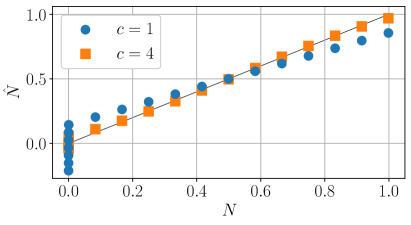
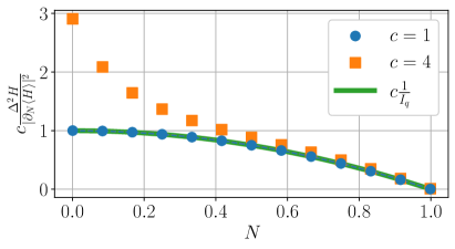
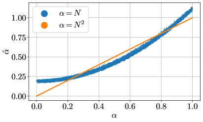
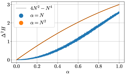
In Fig. 2 we show the negativities of the state (31) predicted by our model. The model was trained on the sets , where are generated from a uniform distribution, and . The model struggles to predict the negativities for , for which . As might be expected, the more copies we process simultaneously, the more accurate our predictions for become. However, in this case the observable (8) requires the measurement of all qubits, for which parameters have to be varied. One could measure fewer qubits , as we did in Section III.1. While it does not worsen the estimation precision for this task, it increases its variance, as we show in Appendix B.1.
Additionally in Fig. 2, we show the variance of the trained observable and the Cramer-Rao bounds (23). As can be seen, the quantum bound is saturated for a single copy of . For both and , our model finds the ansatz angles which provide , but the parameters do not give the desired variance of for . Note that , so the data in the plots are rescaled correspondingly.
III.3 Random pure states
The presented approach aims to be as data-agnostic as possible. In some specific tasks, however, one might also try to augment the method with an extra knowledge about the system. As an example, from entanglement theory an upper bound on the square of the negativity of an arbitrary two-qubit mixed state [77] is known:
| (34) |
where and . Here denotes the projector onto the antisymmetric subspace of the two copies of the -th subsystem. Originally in [77] the bound was derived for the square of another entanglement measure, the concurrence [78, 79, 80]. However, it is known that for the case of two-qubit mixed states the concurrence is always lower-bounded by the negativity [81]. There is also a similar lower bound [82] on the square of concurrence of an arbitrary bipartite state:
| (35) |
where and , with being the projector onto the symmetric subspace of the two copies of the -th subsystem.
The bounds (34), (35) have the form of expectation value of a Hermitian operator with respect to two copies of a given state fitting our approach well. In addition, for pure two-qubit states the bound gives the exact value of squared negativity [77] (and also concurrence and negativity coincide for such states [81]). Thus, we can test the performance of our method on randomly generated pure states and check how well it can variationally find the appropriate observable on two copies to obtain the exact value of the squared negativity. For this task, we trained our regression model on a set consisting of random pure states along with their squared negativities, which are evenly distributed on the interval .
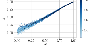
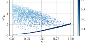
The results depicted in Fig. 3 show that our estimator provides very good predictions for the squared negativity and is able to reproduce numerically two-copy observables like and defined above. For comparison, we additionally plot the results of the performance of our model trained on the same data set, but without squaring the negativities. For both cases, in Fig. 3 we also plot the variance of the optimized observable . For either or in (34) and two copies of a pure two-qubit state with negativity , one can find that which is saturated by found with our method.
III.4 Random mixed states
Prediction of the negativity of random mixed states presents a more challenging problem. To solve it we train our model on a set , where the states are generated such that their negativities are evenly distributed on .
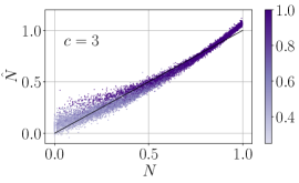
In Fig. 4 we show the predictions of the negativity of randomly generated mixed states by considering copies. Additionally, we indicate the purity of a given state . As can be seen, for lower negativities the states are generally more mixed, which results both in higher estimation error and variance of the optimized observable. Nonetheless, our model performs well even in with a difficult task using a training set of a relatively modest size. However, in this case, our method requires measuring all qubits, which results in additional parameters to vary. Still, our model achieves good prediction accuracy without any knowledge about the connection between the data points and their labels . For comparison, in Appendix B.2 we also show the results obtained for the same training set, but computed with copies. As one could expect, the more copies we process, the better results we get. Following the intuition provided by (34), in Appendix B.3 we apply our method for predicting the squared negativities which results in a significant increase of accuracy for , but giving a little advantage for compared with .
IV Discussion
In this work, using the optimization problem (16) we solve a regression problem for labeled data points represented by quantum states with being the label. The estimate of the label is with being a constructed observable.
Our approach is agnostic to the link between the data points and their labels. In the main text we treat the labels to be an entanglement measure of , an intrinsic property of quantum states. In Appendices, we also apply our method for the cases when with being the ground state of a parametrized Hamiltonian (see Appendix B.4), and where parametrizes a quantum channel acting on some fixed input state (see Appendix B.5).
To assess the performance of our method we employ quantum metrology techniques. Alongside with the prediction accuracy, we also looked at the error propagation (13) and Cramer-Rao bounds (23). For some cases, the proposed method allows to find an observable such that it saturates qCRB. Additionally, by tuning and in (16), one can trade-off between estimation accuracy and its variance, as we demonstrate in Appendix B.4.1.
One of the drawbacks of our method is that there could be no such that its expectation gives the label directly. That is, the estimation given by is generally biased, which sometimes can be mitigated, as we show in Appendix B.4.2. Alternatively, one can seek to find such that it acts on , several copies of the labeled state. As we show in Appendices B.2 and B.5.3, the more copies we process simultaneously, the higher is the estimation accuracy.
In particular we have observed that an estimation of a negativity of random mixed two-qubit states works better in a multi-copy scenario. The prediction gets more accurate with an increase of the number of copies, as can be seen from comparing results for copies (see Appendix B.2). The possible explanation could be devised from recent results on nonlinear multipartite witnesses [83]. The witnesses of this kind are also suited for a multi-copy scenario. In Appendix F we adapt the theory to demonstrate that some specific witnesses show better entanglement detection (averaged over random states) with higher number of copies. Although this is just entanglement detection without estimating any entanglement measure, the inequalities (34) and (35) suggest222In fact, the lower bound in (35) is an example of nonlinear witness. that there might be lower and upper bounds on entanglement measures associated with such witnesses. Also the higher the number of copies is, the tighter and more accurate these bounds are. As a possible direction of further research it would be interesting to establish connections between entanglement measures and multi-copy witnesses.
Among the trainable parameters in (16) there are eigenvalues of the observable . Thus, if the labeled states are of qubits the number of parameters to vary would be exponential. As we discuss in Section II.3 one may search for an observable such that it is enough to measure a fewer number of qubits in some cases. This may be advantageous also in the way that if , then one can have the variational circuit in (9) to be in the form of a QCNN [59, 16] which is known to be immune to barren plateaus [60].
Our work opens new directions for further studies. As such, one can investigate the applicability of QCNNs for regression tasks we consider in this work. In Appendix B.1 for the prediction of the negativity of isotropic states (31) of qubits, we discuss that one can find an observable requiring the measurement of only qubit and providing the same estimation accuracy as that of an efficient observable with , but with about twice greater variance. One might be interested in which regression problems one could obtain an observable of the form (8) which requires a measurement of qubits and provides , but , as we observe for the case of the negativity of isotropic states.
It would be also interesting to consider estimations of some hard-to-compute quantities. For instance, unlike the qubit-qubit case, for mixed qutrit-qutrit states (and also ones of higher dimensions) there is no effective procedure of computing entanglement measures [84]. This is also true for multipartite quantum states, in which case a relevant question is the calculation of various measures [85, 86, 87] of genuine entanglement, i.e., entanglement present in each bipartite cut of a quantum state [88, 89]. In the context of quantum channels, important quantities for transmitting classical and quantum information include channel capacities [90]. The question arises as to how effective the regression method will be in predicting the properties listed above.
V Acknowledgements
The work was supported in the framework of the Roadmap for Quantum Computing (Contracts No. 868-1.3-15/15-2021 and No. R2163).
References
- [1] M. Schuld, I. Sinayskiy, and F. Petruccione. An introduction to quantum machine learning. Contemporary Physics, 56(2):172–185, 2015.
- [2] J. Biamonte, P. Wittek, N. Pancotti, P. Rebentrost, N. Wiebe, and S. Lloyd. Quantum machine learning. Nature, 549(7671):195–202, 2017.
- [3] Seth Lloyd and Christian Weedbrook. Quantum generative adversarial learning. Physical review letters, 121(4):040502, 2018.
- [4] M. Schuld and N. Killoran. Quantum machine learning in feature hilbert spaces. Physical Review Letters, 122(4):040504, 2019.
- [5] K. Mitarai, M. Negoro, M. Kitagawa, and K. Fujii. Quantum circuit learning. Physical Review A, 98(3):032309, 2018.
- [6] Adrián Pérez-Salinas, Alba Cervera-Lierta, Elies Gil-Fuster, and José I Latorre. Data re-uploading for a universal quantum classifier. Quantum, 4:226, 2020.
- [7] Adrián Pérez-Salinas, David López-Núñez, Artur García-Sáez, Pol Forn-Díaz, and José I Latorre. One qubit as a universal approximant. Physical Review A, 104(1):012405, 2021.
- [8] Maria Schuld, Ryan Sweke, and Johannes Jakob Meyer. Effect of data encoding on the expressive power of variational quantum-machine-learning models. Physical Review A, 103(3):032430, 2021.
- [9] Takahiro Goto, Quoc Hoan Tran, and Kohei Nakajima. Universal approximation property of quantum machine learning models in quantum-enhanced feature spaces. Physical Review Letters, 127(9):090506, 2021.
- [10] Patrick Rebentrost, Masoud Mohseni, and Seth Lloyd. Quantum support vector machine for big data classification. Physical review letters, 113(13):130503, 2014.
- [11] Daniel K Park, Carsten Blank, and Francesco Petruccione. The theory of the quantum kernel-based binary classifier. Physics Letters A, 384(21):126422, 2020.
- [12] Leonardo Banchi, Jason Pereira, and Stefano Pirandola. Generalization in quantum machine learning: A quantum information standpoint. PRX Quantum, 2(4):040321, 2021.
- [13] Maria Schuld, Ilya Sinayskiy, and Francesco Petruccione. Prediction by linear regression on a quantum computer. Physical Review A, 94(2):022342, 2016.
- [14] Teppei Suzuki and Michio Katouda. Predicting toxicity by quantum machine learning. Journal of Physics Communications, 4(12):125012, 2020.
- [15] Pranath Reddy and Aranya B Bhattacherjee. A hybrid quantum regression model for the prediction of molecular atomization energies. Machine Learning: Science and Technology, 2(2):025019, 2021.
- [16] Lento Nagano, Alexander Miessen, Tamiya Onodera, Ivano Tavernelli, Francesco Tacchino, and Koji Terashi. Quantum data learning for quantum simulations in high-energy physics. Physical Review Research, 5(4):043250, 2023.
- [17] Vojtěch Havlíček, Antonio D Córcoles, Kristan Temme, Aram W Harrow, Abhinav Kandala, Jerry M Chow, and Jay M Gambetta. Supervised learning with quantum-enhanced feature spaces. Nature, 567(7747):209–212, 2019.
- [18] Carsten Blank, Daniel K Park, June-Koo Kevin Rhee, and Francesco Petruccione. Quantum classifier with tailored quantum kernel. npj Quantum Information, 6(1):41, 2020.
- [19] Sofiene Jerbi, Lukas J Fiderer, Hendrik Poulsen Nautrup, Jonas M Kübler, Hans J Briegel, and Vedran Dunjko. Quantum machine learning beyond kernel methods. Nature Communications, 14(1):517, 2023.
- [20] Marcello Benedetti, Erika Lloyd, Stefan Sack, and Mattia Fiorentini. Parameterized quantum circuits as machine learning models. Quantum Science and Technology, 4(4):043001, 2019.
- [21] M. Schuld, A. Bocharov, K. M Svore, and N. Wiebe. Circuit-centric quantum classifiers. Physical Review A, 101(3):032308, 2020.
- [22] M. Cerezo et al. Variational quantum algorithms. Nature Reviews Physics, 3(9):625–644, 2021.
- [23] Jacob Biamonte. Universal variational quantum computation. Physical Review A, 103(3):L030401, 2021.
- [24] Alberto Peruzzo, Jarrod McClean, Peter Shadbolt, Man-Hong Yung, Xiao-Qi Zhou, Peter J Love, Alán Aspuru-Guzik, and Jeremy L O’brien. A variational eigenvalue solver on a photonic quantum processor. Nature Communications, 5:4213, 2014.
- [25] A. Kandala, A. Mezzacapo, K. Temme, M. Takita, M. Brink, J. M. Chow, and J. M. Gambetta. Hardware-efficient variational quantum eigensolver for small molecules and quantum magnets. Nature, 549:242, Sep 2017.
- [26] A. Kardashin, A. Pervishko, J. Biamonte, and D. Yudin. Numerical hardware-efficient variational quantum simulation of a soliton solution. Physical Review A, 104:L020402, Aug 2021.
- [27] Xiaosi Xu, Jinzhao Sun, Suguru Endo, Ying Li, Simon C Benjamin, and Xiao Yuan. Variational algorithms for linear algebra. Science Bulletin, 66(21):2181–2188, 2021.
- [28] Carlos Bravo-Prieto, Ryan LaRose, Marco Cerezo, Yigit Subasi, Lukasz Cincio, and Patrick J Coles. Variational quantum linear solver. Quantum, 7:1188, 2023.
- [29] R. LaRose, A. Tikku, É. O’Neel-Judy, L. Cincio, and P. J Coles. Variational quantum state diagonalization. npj Quantum Information, 5(1):1–10, 2019.
- [30] Benjamin Commeau, Marco Cerezo, Zoë Holmes, Lukasz Cincio, Patrick J Coles, and Andrew Sornborger. Variational hamiltonian diagonalization for dynamical quantum simulation. arXiv preprint arXiv:2009.02559, 2020.
- [31] Cristina Cirstoiu, Zoe Holmes, Joseph Iosue, Lukasz Cincio, Patrick J Coles, and Andrew Sornborger. Variational fast forwarding for quantum simulation beyond the coherence time. npj Quantum Information, 6(1):82, 2020.
- [32] Jinfeng Zeng, Chenfeng Cao, Chao Zhang, Pengxiang Xu, and Bei Zeng. A variational quantum algorithm for hamiltonian diagonalization. Quantum Science and Technology, 6(4):045009, 2021.
- [33] Bálint Koczor, Suguru Endo, Tyson Jones, Yuichiro Matsuzaki, and Simon C Benjamin. Variational-state quantum metrology. New Journal of Physics, 22(8):083038, 2020.
- [34] Johannes Jakob Meyer, Johannes Borregaard, and Jens Eisert. A variational toolbox for quantum multi-parameter estimation. npj Quantum Information, 7(1):89, 2021.
- [35] Raphael Kaubruegger, Denis V Vasilyev, Marius Schulte, Klemens Hammerer, and Peter Zoller. Quantum variational optimization of ramsey interferometry and atomic clocks. Physical review X, 11(4):041045, 2021.
- [36] Uwe Dorner, Rafal Demkowicz-Dobrzanski, Brian J Smith, Jeff S Lundeen, Wojciech Wasilewski, Konrad Banaszek, and Ian A Walmsley. Optimal quantum phase estimation. Physical review letters, 102(4):040403, 2009.
- [37] Stefano Pirandola, B Roy Bardhan, Tobias Gehring, Christian Weedbrook, and Seth Lloyd. Advances in photonic quantum sensing. Nature Photonics, 12(12):724–733, 2018.
- [38] Senrui Chen, Sisi Zhou, Alireza Seif, and Liang Jiang. Quantum advantages for pauli channel estimation. Physical Review A, 105(3):032435, 2022.
- [39] Juan Carrasquilla and Roger G Melko. Machine learning phases of matter. Nature Physics, 13(5):431–434, 2017.
- [40] Evert PL Van Nieuwenburg, Ye-Hua Liu, and Sebastian D Huber. Learning phase transitions by confusion. Nature Physics, 13(5):435–439, 2017.
- [41] A. V. Uvarov, A. S. Kardashin, and J. D Biamonte. Machine learning phase transitions with a quantum processor. Physical Review A, 102(1):012415, 2020.
- [42] Nana Liu and Patrick Rebentrost. Quantum machine learning for quantum anomaly detection. Physical Review A, 97(4):042315, 2018.
- [43] Jin-Min Liang, Shu-Qian Shen, Ming Li, and Lei Li. Quantum anomaly detection with density estimation and multivariate gaussian distribution. Physical Review A, 99(5):052310, 2019.
- [44] A. Patterson, H. Chen, L. Wossnig, S. Severini, D. Browne, and I. Rungger. Quantum state discrimination using noisy quantum neural networks. Physical Review Research, 3(1):013063, 2021.
- [45] H. Chen, L. Wossnig, S. Severini, H. Neven, and M. Mohseni. Universal discriminative quantum neural networks. Quantum Machine Intelligence, 3(1):1–11, 2021.
- [46] P.-H. Qiu, X.-G. Chen, and Y.-W. Shi. Solving quantum channel discrimination problem with quantum networks and quantum neural networks. IEEE Access, 7:50214–50222, 2019.
- [47] AS Kardashin, AV Vlasova, AA Pervishko, D Yudin, and JD Biamonte. Quantum-machine-learning channel discrimination. Physical Review A, 106(3):032409, 2022.
- [48] Akash Kundu and Jarosław Adam Miszczak. Variational certification of quantum devices. Quantum Science and Technology, 7(4):045017, 2022.
- [49] Joe Gibbs, Zoe Holmes, Matthias C Caro, Nicholas Ezzell, Hsin-Yuan Huang, Lukasz Cincio, Andrew T Sornborger, and Patrick J Coles. Dynamical simulation via quantum machine learning with provable generalization. Physical Review Research, 6(1):013241, 2024.
- [50] Peng-Hui Qiu, Xiao-Guang Chen, and Yi-Wei Shi. Detecting entanglement with deep quantum neural networks. IEEE Access, 7:94310–94320, 2019.
- [51] Claudio Sanavio, Edoardo Tignone, and Elisa Ercolessi. Entanglement classification via witness operators generated by support vector machine. The European Physical Journal Plus, 138(10):936, 2023.
- [52] Lukasz Cincio, Yiğit Subaşı, Andrew T Sornborger, and Patrick J Coles. Learning the quantum algorithm for state overlap. New Journal of Physics, 20(11):113022, 2018.
- [53] Peter D Johnson, Jonathan Romero, Jonathan Olson, Yudong Cao, and Alán Aspuru-Guzik. Qvector: an algorithm for device-tailored quantum error correction. arXiv preprint arXiv:1711.02249, 2017.
- [54] Jan Roik, Karol Bartkiewicz, Antonín Černoch, and Karel Lemr. Entanglement quantification from collective measurements processed by machine learning. Physics Letters A, 446:128270, 2022.
- [55] Kun Wang, Zhixin Song, Xuanqiang Zhao, Zihe Wang, and Xin Wang. Detecting and quantifying entanglement on near-term quantum devices. npj Quantum Information, 8(1):52, 2022.
- [56] Jing Liu, Haidong Yuan, Xiao-Ming Lu, and Xiaoguang Wang. Quantum fisher information matrix and multiparameter estimation. Journal of Physics A: Mathematical and Theoretical, 53(2):023001, 2020.
- [57] Johannes Jakob Meyer. Fisher information in noisy intermediate-scale quantum applications. Quantum, 5:539, 2021.
- [58] Soorya Rethinasamy, Rochisha Agarwal, Kunal Sharma, and Mark M Wilde. Estimating distinguishability measures on quantum computers. Physical Review A, 108(1):012409, 2023.
- [59] Iris Cong, Soonwon Choi, and Mikhail D Lukin. Quantum convolutional neural networks. Nature Physics, 15(12):1273–1278, 2019.
- [60] Arthur Pesah, Marco Cerezo, Samson Wang, Tyler Volkoff, Andrew T Sornborger, and Patrick J Coles. Absence of barren plateaus in quantum convolutional neural networks. Physical Review X, 11(4):041011, 2021.
- [61] Christopher King. The capacity of the quantum depolarizing channel. IEEE Transactions on Information Theory, 49(1):221–229, 2003.
- [62] Nathan Shettell. Quantum information techniques for quantum metrology. arXiv preprint arXiv:2201.01523, 2022.
- [63] Jasminder S Sidhu and Pieter Kok. Geometric perspective on quantum parameter estimation. AVS Quantum Science, 2(1), 2020.
- [64] Luca Pezze, Augusto Smerzi, Markus K Oberthaler, Roman Schmied, and Philipp Treutlein. Quantum metrology with nonclassical states of atomic ensembles. Reviews of Modern Physics, 90(3):035005, 2018.
- [65] Géza Tóth and Iagoba Apellaniz. Quantum metrology from a quantum information science perspective. Journal of Physics A: Mathematical and Theoretical, 47(42):424006, 2014.
- [66] F. Chapeau-Blondeau. Optimized probing states for qubit phase estimation with general quantum noise. Physical Review A, 91:052310, 2015.
- [67] C Huerta Alderete, Max Hunter Gordon, Frédéric Sauvage, Akira Sone, Andrew T Sornborger, Patrick J Coles, and Marco Cerezo. Inference-based quantum sensing. Physical Review Letters, 129(19):190501, 2022.
- [68] Yadong Wu, Juan Yao, Pengfei Zhang, and Hui Zhai. Expressivity of quantum neural networks. Physical Review Research, 3(3):L032049, 2021.
- [69] Zoë Holmes, Nolan J Coble, Andrew T Sornborger, and Yiğit Subaşı. Nonlinear transformations in quantum computation. Physical Review Research, 5(1):013105, 2023.
- [70] V. Vedral, M. B. Plenio, M. A. Rippin, and P. L. Knight. Quantifying entanglement. Phys. Rev. Lett., 78:2275–2279, Mar 1997.
- [71] Ryszard Horodecki, Paweł Horodecki, Michał Horodecki, and Karol Horodecki. Quantum entanglement. Rev. Mod. Phys., 81:865–942, Jun 2009.
- [72] Otfried Gühne and Géza Tóth. Entanglement detection. Physics Reports, 474(1):1–75, 2009.
- [73] C. Eltschka and J. Siewert. Quantifying entanglement resources. Journal of Physics A: Mathematical and Theoretical, 47:424005, 2014.
- [74] J Robert Johansson, Paul D Nation, and Franco Nori. Qutip: An open-source python framework for the dynamics of open quantum systems. Computer physics communications, 183(8):1760–1772, 2012.
- [75] J.R. Johansson, P.D. Nation, and Franco Nori. Qutip 2: A python framework for the dynamics of open quantum systems. Computer Physics Communications, 184(4):1234–1240, 2013.
- [76] Michał Horodecki and Paweł Horodecki. Reduction criterion of separability and limits for a class of distillation protocols. Phys. Rev. A, 59:4206–4216, Jun 1999.
- [77] Cheng-Jie Zhang, Yan-Xiao Gong, Yong-Sheng Zhang, and Guang-Can Guo. Observable estimation of entanglement for arbitrary finite-dimensional mixed states. Phys. Rev. A, 78:042308, Oct 2008.
- [78] Charles H. Bennett, David P. DiVincenzo, John A. Smolin, and William K. Wootters. Mixed-state entanglement and quantum error correction. Phys. Rev. A, 54:3824–3851, Nov 1996.
- [79] William K. Wootters. Entanglement of formation of an arbitrary state of two qubits. Phys. Rev. Lett., 80:2245–2248, Mar 1998.
- [80] Florian Mintert, Marek Kuś, and Andreas Buchleitner. Concurrence of mixed bipartite quantum states in arbitrary dimensions. Phys. Rev. Lett., 92:167902, Apr 2004.
- [81] Christopher Eltschka, Géza Tóth, and Jens Siewert. Partial transposition as a direct link between concurrence and negativity. Phys. Rev. A, 91:032327, Mar 2015.
- [82] Florian Mintert and Andreas Buchleitner. Observable entanglement measure for mixed quantum states. Phys. Rev. Lett., 98:140505, Apr 2007.
- [83] Albert Rico and Felix Huber. Entanglement detection with trace polynomials. Phys. Rev. Lett., 132:070202, Feb 2024.
- [84] Y. Huang. Computing quantum discord is np-complete. New Journal of Physics, 16:033027, 2014.
- [85] Aditi Sen(De) and Ujjwal Sen. Channel capacities versus entanglement measures in multiparty quantum states. Phys. Rev. A, 81:012308, Jan 2010.
- [86] Yue Dai, Yuli Dong, Zhenyu Xu, Wenlong You, Chengjie Zhang, and Otfried Gühne. Experimentally accessible lower bounds for genuine multipartite entanglement and coherence measures. Phys. Rev. Appl., 13:054022, May 2020.
- [87] K V Antipin. Construction of genuinely entangled subspaces and the associated bounds on entanglement measures for mixed states. Journal of Physics A: Mathematical and Theoretical, 54(50):505303, nov 2021.
- [88] George Svetlichny. Distinguishing three-body from two-body nonseparability by a bell-type inequality. Phys. Rev. D, 35:3066–3069, May 1987.
- [89] W. Dür, G. Vidal, and J. I. Cirac. Three qubits can be entangled in two inequivalent ways. Phys. Rev. A, 62:062314, Nov 2000.
- [90] Mark M Wilde. From classical to quantum shannon theory. arXiv preprint arXiv:1106.1445, 2011.
- [91] Ernesto Campos, Daniil Rabinovich, Vishwanathan Akshay, and J Biamonte. Training saturation in layerwise quantum approximate optimization. Physical Review A, 104(3):L030401, 2021.
- [92] Andrea Skolik, Jarrod R McClean, Masoud Mohseni, Patrick Van Der Smagt, and Martin Leib. Layerwise learning for quantum neural networks. Quantum Machine Intelligence, 3:1–11, 2021.
- [93] Tak Hur, Leeseok Kim, and Daniel K Park. Quantum convolutional neural network for classical data classification. Quantum Machine Intelligence, 4(1):3, 2022.
- [94] Marco G Genoni, Paolo Giorda, and Matteo GA Paris. Optimal estimation of entanglement. Physical Review A, 78(3):032303, 2008.
- [95] Jing Liu, Jie Chen, Xiao-Xing Jing, and Xiaoguang Wang. Quantum fisher information and symmetric logarithmic derivative via anti-commutators. Journal of Physics A: Mathematical and Theoretical, 49(27):275302, 2016.
- [96] Leonid Gurvits. Classical deterministic complexity of edmonds’ problem and quantum entanglement. In Proceedings of the Thirty-Fifth Annual ACM Symposium on Theory of Computing, STOC ’03, page 10–19, New York, NY, USA, 2003. Association for Computing Machinery.
- [97] Charles H. Bennett, Herbert J. Bernstein, Sandu Popescu, and Benjamin Schumacher. Concentrating partial entanglement by local operations. Phys. Rev. A, 53:2046–2052, Apr 1996.
- [98] Michał Horodecki, Paweł Horodecki, and Ryszard Horodecki. General teleportation channel, singlet fraction, and quasidistillation. Phys. Rev. A, 60:1888–1898, Sep 1999.
- [99] Luca Pezzé and Augusto Smerzi. Entanglement, nonlinear dynamics, and the heisenberg limit. Phys. Rev. Lett., 102:100401, Mar 2009.
- [100] A. Peres. Separability criterion for density matrices. Physical Review Letters, 77:1413, 1996.
- [101] K. Życzkowski, P. Horodecki, A. Sanpera, and M. Lewenstein. Volume of the set of separable states. Physical Review A, 58:883, 1998.
- [102] G. Vidal and R. F. Werner. Computable measure of entanglement. Physical Review A, 65:032314, 2002.
- [103] M. Horodecki, P. Horodecki, and R. Horodecki. Separability of mixed states: necessary and sufficient conditions. Physics Letters A, 223:1, 1996.
- [104] S. Lee, D.-P. Chi, S.-D. Oh, and J. Kim. Convex-roof extended negativity as an entanglement measure for bipartite quantum systems. Physical Review A, 68:062304, 2003.
- [105] Jens Eisert. Entanglement in quantum information theory. arXiv preprint arXiv:quant-ph/0610253, 2006.
- [106] Aram W. Harrow. The church of the symmetric subspace. arXiv preprint arXiv:quant-ph/1308.6595, 2013.
Appendix A Hardware-efficient ansatz
In this work, we represent the parametrized quantum circuit by the so-called hardware-efficient ansatz (HEA) [25, 26]. The idea behind such ansätze is in alternation between single-qubit rotations and operations capable of introducing entanglement into the system. In our implementation, an example of which is shown in Fig. 5, the ansatz consists of several layers of parametrized gates. Each layer contains an array of - and - of Pauli rotations acting on individual qubits, followed by a cascade of controlled -rotations which produce entanglement. In our ansatz, we also have the “zeroth layer” containing no entangling gates. Therefore, the total number of the parameters in an -qubit -layered ansatz is .
As one may notice, all gates in the ansatz are parametrized. This could be helpful for applying optimization techniques such as layerwise training [91, 92]. That is, having trained an ansatz of layers, one adds another layer with the parameters initialized to zeros, and continues the training of the resultant -layered ansatz. Similarly, in our setting one could first train the ansatz for copies of a state , add another copy, correspondingly add new gates to the ansatz with the parameters set to zeros, and continue the optimization for .
In Section II.3, we discussed measurements of out of qubits of the transformed state for reduction of the number of parameters in (8) from to . For such a purpose, one can represent in the form of a so-called quantum convolutional neural network (QCNN) [59, 93, 16]. A QCNN can be viewed as a sequence of convolutional layers, which usually consist of two-qubit gates acting on neighboring qubits, and pooling layers, in which one traces out a subset (usually, a half) of qubits. At the end of the QCNN, one measures an observable of interest on the remaining qubits. In Fig. 6, we show an example of a QCNN for a state of qubits and an observable of the form (8) for measured qubit.
Despite allowing to have fewer parameters in both and , it is not always advantageous to measure qubits, even if the corresponding observable gives . In Appendix B.1, we consider a regression task in which, if one measures qubit, one gets the variance about twice as large as if measuring qubits.
Appendix B Additional results
Here we provide additional results of numerical application of our method for predicting the negativity with various conditions (e.g., using fewer copies of the labeled state), and for solving other regression tasks, such as estimating the angle of a Pauli rotation, and predicting the strength of transverse field for the Ising Hamiltonian.
B.1 Measuring fewer qubits while predicting the negativity of isotropic states
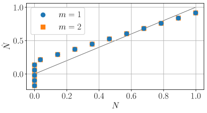
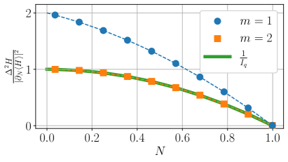
In Section III.2, we studied the performance of our method in predicting the negativity of isotropic states (31). As we noted, to achieve better results, we need to measure all qubits of the state . However, we found that if one measures fewer qubits (thus decreasing the number of variational parameters see (8))the estimation accuracy does not decrease, but increases its variance. We demonstrate this in Fig. 7 for , where we show the variances of the optimized observable for and . As can be seen, when we measure only one qubit, the variance is about twice as large as if we measure both qubits.
A possible explanation of this could be as follows. When we measure only of qubits, the observable (8) has the form , where are two-dimensional projectors, and the eigenvalues are twice-degenerate. At the meantime, the efficient observable (33) has two distinct eigenvalues as well, but one unique with the value and one thrice-degenerate with the value . For this particular case, this degeneracy may be important and cannot be accounted by our method.
Potentially, this may limit the application of QCNNs for regression tasks such as considered in this work. Indeed, after the application of a QCNN, it is supposed that one measures a local (e.g., single-qubit) observable. In our setting, we vary the eigenvalues , but cannot vary their degeneracy (or the dimensionality of the eigenprojectors ), which may be crucial, as discussed above.
For , our method finds an observable with and . Consider, for example, where are any vectors perpendicular to and to each other. For this observable and an isotropic state of the form (32), one can verify that and , which coincides with the blue line in Fig. 7 (right). For , this variance is greater than qCRB which is saturated by (33).
B.2 Predicting the negativity of random mixed states with fewer copies
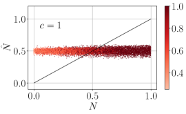
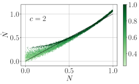
In Section III.4, we applied our method for predicting the negativity (28) of random mixed two-qubit states. To train the model, we processed copies of the labeled state simultaneously. Here we show how the performance of our method changes with processing a fewer number of copies. To train the model, as before, we generated a training set of random states with negativities evenly distributed on . Additionally, having trained the model with copies, we use the optimal parameters as the initial ones for training the model with copies.
In Fig. 8 the results of predicting the negativity of mixed states for are shown. Interestingly, the model trained with only a single copy does not allow to predict anything. In contrast, with two copies, the estimation accuracy is much higher which is in line with our reasoning in Section III.3. With three copies, the performance does not improve much in comparison to the case with two copies. Finally, with copies, as we show in Section III.4, the prediction accuracy increases significantly.
B.3 Predicting the squared negativity of random mixed states
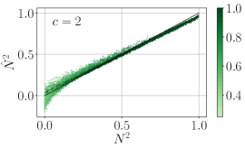
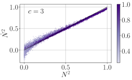
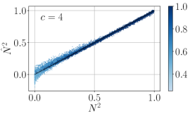
In Section III.3 we have shown that one can predict the squared negativity of pure states using our method. In this Appendix we test the performance of the method in predicting as well, but for random mixed states. In Fig. 9, we show the estimation accuracy for this case for copies of the labeled state. Interestingly, while with copies the prediction accuracy is quite high, the performance does not increase much for . In contrast, with , the estimation of is very precise, especially for more pure states. With copy, we obtained the results similar to the ones presented in Fig. 8(left) (not shown here).
B.4 Predicting transverse field of Ising Hamiltonian
We numerically apply our approach for estimation of the transverse field of the Ising Hamiltonian
| (36) |
where , are Pauli operators acting on the th qubit, and we apply the periodic boundary conditions . Thus, given a collection of the ground states of in the form (1) one wishes to solve (16) finding the observable such that the expectation gives an estimation of the transverse field . In our numerical experiments we consider qubits and set .
B.4.1 Dependence on weights and
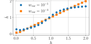
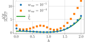
In Section II.4 we mentioned that by adjusting the weights and in (1), we can trade-off between the accuracy of the estimation and its variance. In Fig. 10, we show the results of predicting the transverse field of (36) with setting and considering and . As might be expected, the greater is the weight , the less accurate predictions we get. However, with , we almost saturate qCRB (23).
B.4.2 Compensation of a bias
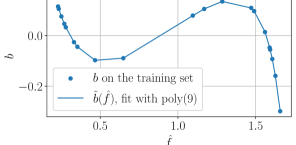
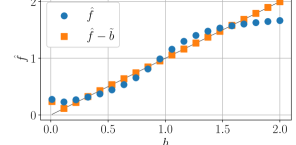
As is noted in Section II.6, generally evaluates to some function instead of itself. There is a bias which one can try to compensate. Indeed, after the training, we can observe the bias for . One can plot the dependence of on the obtained predictions . If this dependence is monotonic the data points can be fitted with some function (e.g., polynomial of some degree), which we denote . This function can then be used for processing the predictions for unseen data.
In Fig. 11 we show the results of testing this bias compensation method for the task we considered in the previous section, where we predicted the transverse field of the Ising Hamiltonian. As can be seen, the values give very accurate predictions, except for a small interval on the left where happens to be non-monotonic.
B.5 Predicting channel parameter
Here our method is applied for learning to predict the parameter of a parametrized channel , i.e. the labeled states have the form for some fixed input state .
B.5.1 Depolarizing channel
The first channel under our study is the single-qubit depolarizing channel
| (37) |
which we have already considered in Section II.4. Representing the input state as with , one can find the (unnormalized) eigenvectors of the SLD operator of the output state to be
which do not depend on the label . Therefore, a POVM which saturates qCRB (23) should not depend on as well. Let us set the input state to . For this input, one can obtain the SLD operator for the output as
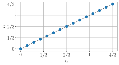
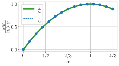
which, by formula (22), gives . Please, note the equality of this to the reciprocal of (12) with . In Fig. 12, we show the performance of our method in predicting for the depolarized state . As can be seen, trained on a set of five states with random depolarization strengths , our model finds an observable giving both accurate predictions and variance saturating the qCRB.
B.5.2 Amplitude damping channel
Now we consider the amplitude damping (AD) channel
| (38) |
with the Kraus operators
This is a single-qubit channel which models the decay from the excited state to the ground state [90].
Let us consider the input state for this channel in the Bloch representation
where with . The output state of the channel therefore reads
| (39) |
where is the output state Bloch vector with the components
| (40) |
Let us assume that , then by formula (58) we obtain the following structure of the SLD operator:
| (41) |
where
| (42) |
with , and the components of the vector are
| (43) |
The eigenvector decomposition of reads
| (44) |
where and
with such that . More explicitly,
| (45) |
where
| (46) |
Let us consider two input states for the amplitude-damping channel. First, if , then the input is the maximally mixed state , for which Eqs. (45) and (46) yield
| (47) |
with the eigenprojectors of not depending on , and giving . Second, if , which corresponds to , the eigenvectors of the SLD operator (45) are characterized by the vector , which in this case has components
| (48) |
The eigenvalues of the SLD operator are
| (49) |
Using (60), one also obtains .
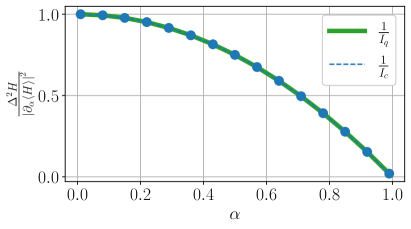
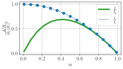
Let us look how our model predicts the amplitude-damping channel parameter for . For both above-mentioned inputs and , we find observables which give accurate predictions of . Interestingly, for either of the inputs, a simple observable gives . Moreover, for , this observable saturates qCRB, which can be verified by combining (47) and (24). In contrast, is not optimal for in the sense of the variance. As can be seen in Fig. 13, our model does not find an observable saturating qCRB in this case. From (45) and (46), one can notice that the eigenprojectors of depend on the parameter . If the optimal POVM tends to , while at the other end of the parameter range, , the optimal POVM is .
B.5.3 Unitary transformation
Let us consider a unitary channel which performs the -rotation of a single-qubit state by an angle :
| (50) |
Such transformation is often considered in the area of quantum channel estimation and quantum metrology as it incarnates, e.g., the Ramsey interferometry [64]. The main obstacle for us in estimating the label for with our method is that we cannot directly obtain as the expected value of some observable . Instead, as noted in SectionII.6, our estimation is generally biased. The function has an estimation which one would obtain in experiments [62]. However, one can suppress this bias by training an observable acting on a number of copies of the labeled state.
Indeed, let and consider copies of this state passed through the channel (50):
where in the last line is the rest of terms to complete . From this expansion, one can guess an observable such that
| (51) |
which is precisely the first terms of the Fourier series of the function . Indeed, if we take
| (52) |
then we get
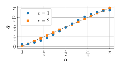
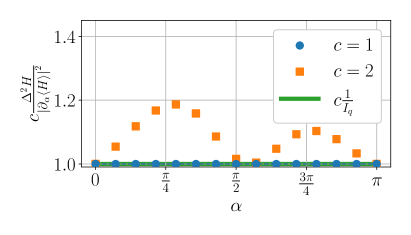
Therefore, we can expect that the more copies of the state we process simultaneously, the more is closer to (i.e. the lower is the estimation bias). This is what happens if we apply our method for predicting the rotation angle in (50),with the results shown in Fig. 14. As can be seen, already with a single copy () we obtain quite an accurate estimation for , which significantly improves with copies. However, in contrast to the single-copy case, with two copies we do not saturate CRB (23).
For a more general one-qubit unitary transformation
| (53) |
with being an arbitrary function of parameter and the generator of rotation around the axis parallel to a given fixed unit vector , one can single out the properties that affect the estimation error. Indeed, let the input state be given by the Bloch representation . One can use Eqs. (22) and (56) to calculate qFI of the output state:
| (54) |
where is the derivative of with respect to and is an angle between vectors and . From this expression, it can be seen that the effects of functional dependence on the parameter and mixedness of the input state are isolated in the factors and , respectively. Since qFI appears in the denominator of the qCRB (23), these two factors significantly affect the estimation error . In particular, the case of highly mixed input states () is expected to require higher number of measurements in comparison with pure case to achieve reasonable values of the estimation error.
Appendix C Some formulas for SLD operator and quantum Fisher information
For an -qubit state , qFI can be calculated as , where the SLD operator was defined in Eq. (21). Although defined implicitly, can be expressed in the basis of as
| (55) |
where the summation is taken over the indices and such that [56, 94]. If possesses certain properties, one can obtain more conveniently [95]. For a mixed single-qubit state, one can write
| (56) |
Additionally, if , then . For a pure state , the SLD operator is simply
| (57) |
Finally, for a single-qubit state in the Bloch representation , where and , one can use the following expression [66]:
| (58) |
It is also possible to obtain the qFI directly without calculating the SLD operator. For instance, the following expression is especially useful for numerical calculations
| (59) |
where in the numerator we have the fidelity between quantum states and [63, 37]. Additionally, if is full-rank, one can also obtain the qFI as [56]
| (60) |
Finally, for a pure state , qFI is
Appendix D Mean squared error and Cramer-Rao bound for biased estimators
In Section II.6, we mentioned that for a given the estimator of can be biased. In this Appendix following the works [62, 63], we derive the expressions for the MSE (25) and cCRB (26) for a biased estimator.
First, let us introduce a bias into our estimate,
| (61) |
where we have a bias and an observable in the form with the operators forming a POVM, and . Denoting , we can rewrite (61) as
Now, suppose that we perform measurements for obtaining this expectation value in an experiment. Each measurement result in an outcome which is observed with probability . Hence, the estimation of can be written as
In this expression, are independent and identically distributed (i.i.d.) random variables, each on average giving for all . Then as in (61). The MSE of the estimation is
In the derivation above, we used the property of i.i.d. random variables that for .
So, we have an expression of the error of the estimation . However, after training and testing the model, one would observe neither nor , but rather , i.e., the error between the estimation and the labels from the training set. One can obtain it after the following chain of transformations:
where we have inserted the bias from (61) at the end. Now, since we obtained , we can write
which is the equation (25). Finally, recalling the error propagation formula (13) and cCRB (19), as well as noticing that
we arrive to the desired inequality (26):
Interestingly, from one can also obtain
which can be used for estimating the classical Fisher information . Indeed, having trained the observable , one obtains the variances via measurements according to (15), and the bias is observed on the labels from the training set . Therefore, if the training set size is sufficiently large, and the labels are distributed uniformly, then one could try to approximate via finite differences. As an instance, for and assuming , the central difference approximation would be
Appendix E Bipartite entanglement
Consider a bipartite state defined on Hilbert space . The state is called separable if it can be represented by an ensemble of product states
| (62) |
with and defined on and , respectively.
A bipartite state is called entangled if it is not separable. In general, it is hard to determine whether a given mixed state is entangled or separable even if one has full access to its density operator [96].
Entanglement measures [70, 71, 72, 73] are used to quantify, in some sense, the amount of entanglement present in quantum states. A number of measures have been introduced, but only few of them have clear operational meaning and direct relation to protocols of quantum information processing [97, 78, 98, 99]. Nevertheless, even abstractly introduced measures are able to show the presence of entanglement in the sense that they vanish on separable states and take non-zero values on entangled ones. It was shown that computation of such entanglement measures for general states in high dimensions is NP-complete [84].
One of the most efficient theoretical ways to detect entanglement in a bipartite state is to analyze its partial transpose [100]. The partial transpose operation with respect to party is defined by its action on elementary operators as
| (63) |
and is extended on arbitrary operators by linearity. If a state is separable, i.e., is of the form (62), then its partial transpose is necessarily positive, i. e. the state satisfies the positive partial transpose (PPT) condition. Consequently, if has at least one negative eigenvalue, i.e. the state violates PPT condition, then its entanglement is detected (PPT criterion). The entanglement quantifier, which is related to this approach, is called negativity [101, 102] and is defined as
| (64) |
where is the trace norm of .
It is known that the PPT condition is necessary and sufficient for separability of qubit-qubit and qubit-qutrit quantum states [103]. For higher dimensions, there are entangled states with positive partial transpose and, correspondingly, vanishing negativity. In this respect, the negativity is a faithful entanglement measure only for qubit-qubit and qubit-qutrit cases. While the definition of negativity can be modified to detect all mixed entangled states also in higher dimensions [104], we use expression (64) because of its practicality and simplicity for the qubit-qubit case, the only case we concentrate on in the present work.
For the qubit-qubit case there is another expression [105] for negativity:
| (65) |
where is the smallest eigenvalue of .
Appendix F Average performance of nonlinear entanglement witnesses with many copies
Here we use the results of Ref. [83] to get insight into the effect of multiple copies on detecting entanglement.
A linear witness is a Hermitian operator (observable) such that for all separable states and for some entangled states that are detected by this witness. In a multi-copy scenario, one can consider nonlinear witness such that for all separable states and for some entangled states . Such a witness is constructed as a tensor product of linear witnesses:
| (66) |
where input and output dimensions of states and witnesses should match. As an example, for copies of a bipartite state the structure of will be
| (67) |
and the average of the observable with respect to copies of is
| (68) |
In Ref. [83] it has also been observed that some of the linear witnesses in (66) can be replaced with specific positive operators , and the resulting nonlinear witness might get even stronger.
In order to consider average performance on random pure bipartite states we follow the lines of Appendix F of Ref. [83] and make special choice of operators and in eq. (67). The first one will be
| (69) |
where is the projector onto the antisymmetric subspace of Hilbert space of parties , and the second one, , is set just to the projector , which is a positive operator. Note that for copies the resulting nonlinear witness is proportional to the lower bound on squared concurrence in (35).
The average over copies of Haar-random states , with ( for qubits), reads
| (70) |
and the well-known expression [106] can be used:
| (71) |
where is the projector onto the symmetric subspace of Hilbert space of parties, each of dimension .
Calculation of (70) with the use of (71) yields (Ref. [83], eq. (F10)):
| (72) |
where - the projector onto the anti-symmetric subspace of Hilbert space of parties, each of dimension (here we assume that ). One cannot use (72) for arbitrarily large number of copies , since
| (73) |
is the dimension of the antisymmetric subspace of parties with local dimension , and the projector vanishes when . Therefore, for two-qubit states, i. e., when , the number of copies is limited by . Nevertheless, the following argument can be used. One can take bipartite states with local parties of sufficiently large dimensions and and then ”split” each local dimension into a tensor product of smaller ones. Let us say, , then each such subsystem can be split into one-qubit systems. If the initial state factorizes, under splitting operation, into tensor product of identical two-qubit states, then using copies of will result in copies of some two-qubit state. Note also that in this case the entanglement of the initial state is fully determined by the entanglement of its factors. Of course, not every pure state factorizes under splitting operation exactly into a tensor product of states with smaller local dimensions, but averaging in (70) is performed over Haar-random states, and this set includes those states that factorize. The simplest example of a factorizable entangled state is the Bell’s state of dimension
| (74) |
where the parties and of dimension are split into -dimensional parties and , and , respectively. Splitting results in two identical Bell’s states of smaller dimension .
Now we can use eq. (72) for copies, and, consequently, . Averaging over such Haar-random pure states includes those that can be factorized into identical two-qubit states. The factorization results in copies of such states. The reason why eq. (72) still holds after splitting is that trace in eq. (70) is stable under such an operation. When , the averaging is performed over the set which includes copies of identical two-qubit states and results in expression
| (75) |
Starting from the value at ( copies), the average monotonically decreases and tends to when . This decreasing of the average value of entanglement witness over random states suggests that entanglement detection becomes more effective with the increase of number of copies of two-qubit states. We can then conjecture that, when working with many copies of states, the regression model variationally finds observables like those in eqs. (67), (69) or maybe even more optimal ones connected with some tight bounds on entanglement measures. This could potentially explain the increase of negativity estimation accuracy on copies of states which is seen on Fig. 4.