Local Clustering for Lung Cancer Image Classification via Sparse Solution Technique

Jackson Hamel¹¹1jrhamel314@uga.edu. Department of Mathematics, University of Georgia, Athens, GA 30602. Ming-Jun Lai²²2mjlai@uga.edu. Department of Mathematics, University of Georgia, Athens, GA 30602. This author is supported by the Simons Foundation Collaboration Grant #864439. Zhaiming Shen³³3zhaiming.shen@uga.edu. Department of Mathematics, University of Georgia, Athens, GA 30602. Ye Tian⁴⁴4yt95681@uga.edu. Department of Mathematics, University of Georgia, Athens, GA 30602.

Abstract

In this work, we propose to use a local clustering approach based on the sparse solution technique to study the medical image, especially the lung cancer image classification task. We view images as the vertices in a weighted graph and the similarity between a pair of images as the edges in the graph. The vertices within the same cluster can be assumed to share similar features and properties, thus making the applications of graph clustering techniques very useful for image classification. Recently, the approach based on the sparse solutions of linear systems for graph clustering has been found to identify clusters more efficiently than traditional clustering methods such as spectral clustering. We propose to use the two newly developed local clustering methods based on sparse solution of linear system for image classification. In addition, we employ a box spline-based tight-wavelet-framelet method to clean these images and help build a better adjacency matrix before clustering. The performance of our methods is shown to be very effective in classifying images. Our approach is significantly more efficient and either favorable or equally effective compared with other state-of-the-art approaches. Finally, we shall make a remark by pointing out two image deformation methods to build up more artificial image data to increase the number of labeled images.

Key words: Graph Laplacian, Image Simplification, Local Clustering, Lung Cancer Image Classification, Sparse Solution Technique

1 Introduction

Lung cancer is one of the most common, and one of the deadliest cancers; only about $17\%$ of people in the U.S. diagnosed with lung cancer survive five years after the diagnosis. Currently, diagnostic methods to detect this cancer include biopsies and imaging, like CT scans. Given the severity of the cancer, early detection significantly improves the chances for survival, but it is also more difficult to detect early stages of lung cancer as there are typically fewer symptoms. To add to the difficulty and complexity, when imaging techniques display cancerous-looking growths, they could either be benign (not harmful) or malignant (harmful). Thus, our task is a ternary classification problem to detect the presence of lung cancer in a patient’s CT scans and determine whether a growth is benign or malignant.

We are interested in lung cancer image classification and providing a complementary method to help computer-aided clinic diagnosis (CACD). More precisely, we would like to help improve the computational feasibility, interpretability, and robustness of the existing methods in image-based CACD. The medical image analysis for lung cancer classification involves two types of approaches: traditional machine learning algorithms, which classify cancer based on manually extracted features from the images, and deep learning techniques, which automatically learn and extract features directly from the raw images. So far, the most popular methods to classify images are based on neural network structures such as ResNet50, EfficientNetB0, InceptionV3, MobileNetV2, DenseNet121, ResNet101, VGG18. See, e.g., [Z21], [HM18], [Al21], [Raza23] for more details. In addition, topological machine learning algorithms such as [A23] and [Y23] were recently developed to provide additional competitive and complementary methods. There are many other algorithms available in the literature and existed online.

The primary objective of this study is to detect cancerous cells in lung nodule CT scan images. It aims to classify lung cancer into three distinct categories: benign, malignant, and normal, based on CT scan slices of lung nodules. To accomplish this task, we propose to use a simple yet effective local clustering approach based on the sparse solution of linear system for image classification. Our idea is based on the methods recently developed in [LM20],[LS23], [LS23b]. See [Shen24Diss] for a comprehensive study of these methods.

The main idea of these methods is that we view a set of image data as a graph $G$ whose vertices are associated with images. Images in the same cluster are in the same class, e.g. benign, or malignant or normal. Given a testing (query) image, we look for a cluster, usually of a small size, which contains the query image as the seed. For example, suppose the output cluster (excluding the query image) is of size 6, then if all 6 images belong to one of the three classes, say malignant, the query image is concluded to be a malignant image. Of course, we can also use a weaker criterion: the testing image is malignant if 3 out of the 6 images are malignant, 2 out of the 6 images are benign, 1 out of the 6 images are normal.

To perform the clustering task, the first and foremost step is to build up an effective adjacency matrix for the group of training images. There are a lot of distance functions we can use. As one needs to find the best one in the sense that for the graph only based on labeled sample images, the adjacency matrix should have a block diagonal structure after the permutation according to the class membership. The way to generate a good adjacency matrix is introduced in Section 3 with more details. We will also present a box spline based on tight-wavelet frames (TWF) to simplify all the images by removing some redundant information away so that the adjacency matrix built by a traditional modified exponential distance (cf. [ZP04]) is much cleaner. The idea about image simplification is explained in Section 2.

After building up the adjacency matrix, we simply form its graph Laplace matrix and use our local clustering techniques based on sparse solutions of linear system (cf. [LW21]). Our idea can be explained as follows. Letting ${\bf c}_{1}$ be the indicator vector of cluster $C_{1}$ whose entries are 1 associated with the vertices in the cluster $C_{1}$ , and 0 otherwise. It is easy to see that ${\bf c}_{1}$ is a sparse vector. For example, the cluster $C_{1}$ may have $\|{\bf c}_{1}\|_{0}=5$ while the total number of images is possibly $N\gg 1000$ . Thus, the number of nonzero entries in $C_{1}$ , i.e. $\|{\bf c}_{1}\|_{0}$ is much smaller than the size $N$ of the graph. Since we have

{\cal L}{\bf c}_{1}=0,

(1)

where ${\cal L}$ is the graph Laplacian of the graph $G$ (cf. [C97]), we cast the problem of finding ${\bf c}_{1}$ as a minimization problem

\min\|{\bf x}\|_{0},\ {\cal L}{\bf x}=0,\ {\bf x}\neq{\bf 0},

(2)

where $\|{\bf x}\|_{0}$ stands for the number of nonzero entries in ${\bf x}$ . This problem was studied two decades ago (cf. [Candes06] and [Donoho06]) as a compressive sensing problem. See also [LW21] for a detailed explanation. In this paper, we will present two computational algorithms specific to the local clustering problem for identifying lung cancer images. See Section 4 for a detailed explanation.

We shall first demonstrate the effectiveness of these two computational algorithms in categorizing images of various human faces based on two well-known human face datasets: AT&T and YaleB human face data. Then we will show the proposed two algorithms work well for the medical image datasets we studied in this paper. One of the major advantages of our approach is its computational efficiency, as our approach only involved in finding a sparse solution of the linear system associated with the graph Laplacian matrix. It does not need to compute the eigenvectors of the graph Laplacian matrix, which will be more costly when the size of the image data is large. Our numerical experiment can be done in minutes while a convolutional neural network requires hours or more. We summarize our experimental results in Section LABEL:secExp.

The goal of our research is to determine a testing image as one of the three classes: Benign, Malignant, or Normal. Let us first summarize our computational procedure as follows:

•

Preprocess the images by rescaling the images to the same size and applying a Gaussian blur algorithm to reduce the high-frequency components of these images.
•

Simplify these images by using, e.g. PCA, TWF, Watershed, etc..
•

Build up an adjacency matrix $A$ by using, e.g. K-NN, $L^{2}$ distance, modified exponential distance.
•

For each testing image, we use either one of the two proposed local clustering methods, Local Cluster Extraction (LCE) or Least Squares Clustering (LSC), to find a small cluster of images which are similar to the given testing image.
•

Make conclusion about the label of the testing image based on the majority vote of the labels of the images in the found small cluster.

We shall explain these steps of computation in the following sections. The main contributions of this work are the following:

•

We propose to use an approach based on the idea of sparse solution technique for local clustering in order to identify a given test image is benign, malignant, or normal.
•

We treat each image as a vertex in the graph, and use modified exponential distance to build the adjacency matrix between all pairs of images. Then we apply LCE or LSC for medical image classification (identification).
•

The image is preprocessed by applying a box spline based tight-wavelet frames method, with edgeS being detected and enhanced.
•

The experiments demonstrate that our image classification is fast and accurate, and hence can be served as a complementary method to help CACD.

However, we notice that the size of the data set we are using is small, about 1097 images. In order to achieve a better result, we can increase the size of the labeled data. We will propose two approaches: one is based on the solution of the optimal transport problem, i.e. a numerical approximation of the minimizer based on the solution of Monge-Ampére equation studied in [LL24] to help generate more labeled images. The other approach is based on harmonic generalized barycentric coordinates (GBC) for image deformation (cf. [DHL22]). We will show a few examples to illustrate the GBC approach for generating more labeled images in the end of the paper while leaving the entire computation of generating new images to the future work. Nevertheless, we will remark in Section LABEL:secRemark to convince the readers that this approach will generate enough labeled data.

2 Image Simplification

It is crucial to simplify the images, so that we can keep the important features in an image while removing the noises before we feed them into any machine learning model for image classification. It is well-known that we can use the standard PCA to simplify an image. In fact, we have tried to use the first 10 singular values of each image to build up an adjacency matrix $A$ , however, it turns out that the numerical results of image classification based on PCA simplication does not work very well. We thus turned to other approaches.

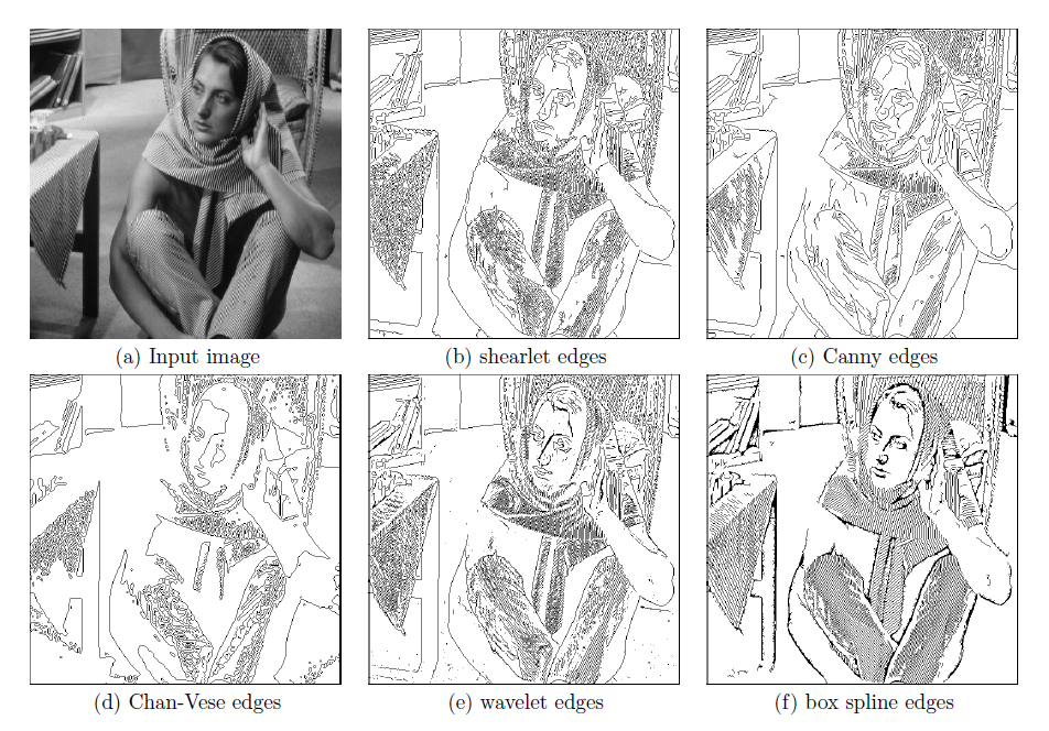
Refer to caption — Figure 1: An example of image simplification by using box spline based tight-wavelet frames courtesy of Ming-Jun Lai, an author of [GL13].

We now explain the box spline-based tight-wavelet frames, called LN method, to simplify these images. The tight wavelet frames (TWF) we used in this paper were constructed in [N05] based on integer translations of box spline $B_{2211}$ (cf. [BHR93] and [LS07]). Dr. Kyunglim Nam implemented the constructive method in [LS06] based on box spline $B_{2211}$ to construct tight-wavelet framelets for image decomposition and reconstruction. In fact, she constructed tight-wavelet frames based on other box splines. See her dissertation [N05] for more detail. Her MATLAB codes were further revised by Dr. Ming-Jun Lai with a denoising technique to have a package called LNmethod.m. As shown in Figure 1, we can easily see the box spline-based tight-wavelet frames method outperforms other traditional edge detection approaches and is able to capture and enhance the edge features across all directions in the image. More recent study can be found in [GL13].

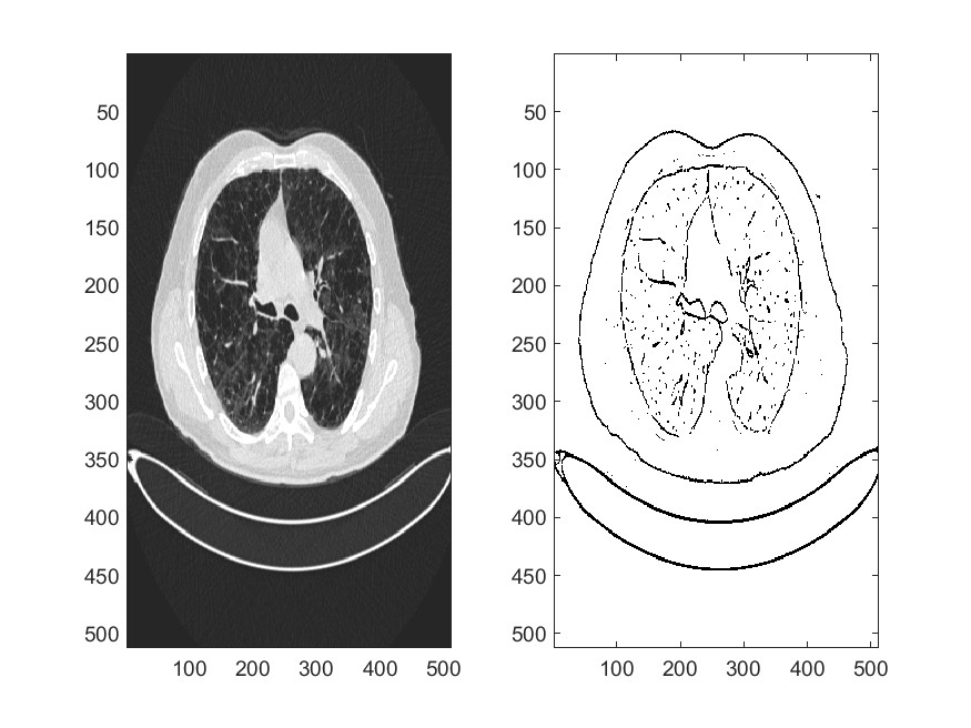
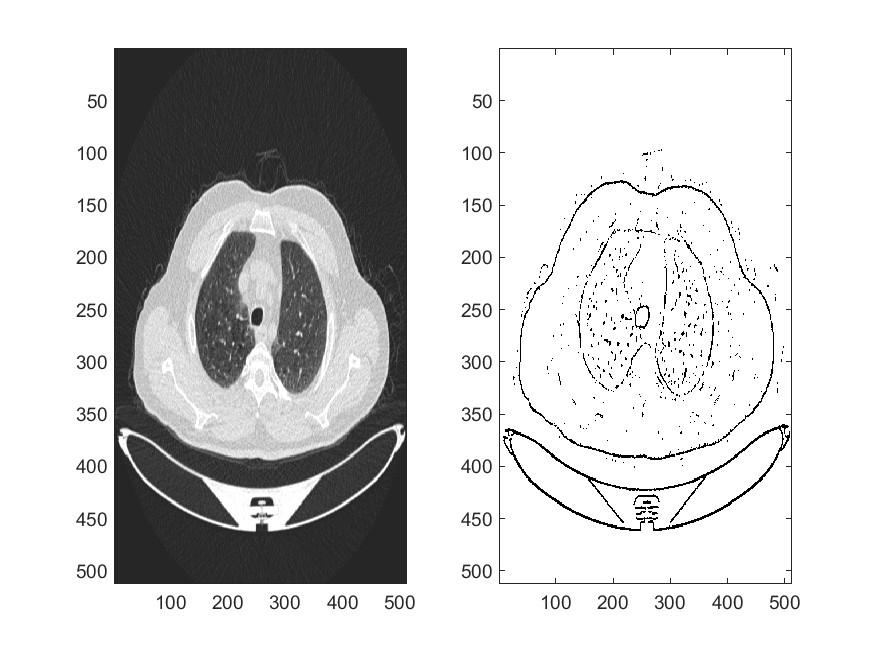
The main idea of LN method is to decompose an image into its low frequency part and high frequency part by using the tight-wavelet frames and then reconstruct the high frequency part back based only on the high-pass frequency part without the low-pass frequency. The resulting image is noisy and is denoised by using a cutoff parameter which is dependent on each image. We find an intelligent way to let the computer decide the best parameter to clean each of the medical images of interest. Let us present some examples of medical image simplification by using the LN method in Figure 2.

3 Generation of Adjacency Matrices

Let us now explain the way we build the adjacency matrices for our graph clustering approach. We mainly use the distance associated with Gaussian kernel with different parameters to generate a working adjacency matrix. Let us call it Modified Exponential Distance:

Let ${\bf x}_{i}\in\mathbb{R}^{n}$ be the vectorization of each image from the original data set and $NN({\bf x}_{i},K)$ is the set of K-nearest neighbors of ${\bf x}_{i}$ . For $r\geq 1$ , let $\sigma_{i}=\|{\bf x}_{i}-{\bf x}^{i,r}\|$ be the $r$ -th closest point of ${\bf x}_{i}$ . We build the adjacency matrix associated with the data set to be $A=[A_{ij}]_{i,j=1,\cdots,n}$ with entries

A_{ij}=\left\{\begin{array}[]{cc}\exp(-\|{\bf x}_{i}-{\bf x}_{j}\|/(\sigma_{i}\sigma_{j})&\hbox{ if }{\bf x}_{j}\in NN({\bf x}_{i},K)\cr 0&\hbox{otherwise }\end{array}\right.

(3)

for all $i,j=1,\cdots,n$ (cf. [ZP04]).

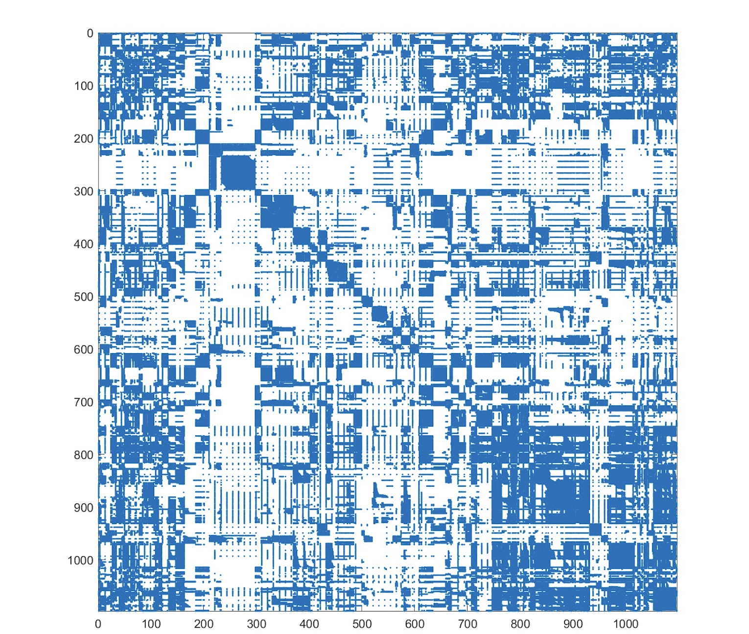
Note that the above $A_{ij}$ is not necessarily symmetric, so we consider $\tilde{A}_{ij}=A^{\top}A$ for symmetrization. Alternatively, one may also use $\tilde{A}_{ij}=\max\{A_{ij},A_{ji}\}$ or $\tilde{A}_{ij}=(A_{ij}+A_{ji})/2$ .

Based on the modified exponential distance (3), we generate the adjacency matrix with the choice of two parameters $r$ and $K$ over all the images. The ideal adjacency matrix would have a block diagonal structure where each block corresponds to one class in the dataset.

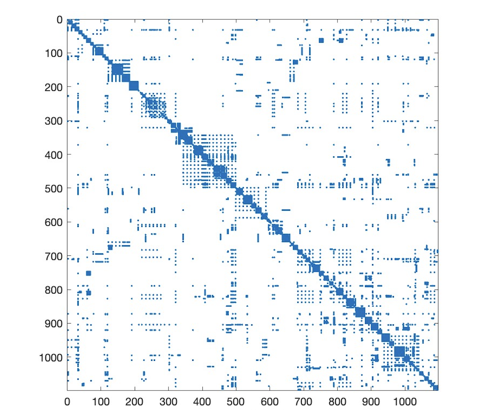Once we have the way to generate the adjacency matrix, we can use the LN method explained before to simplify the given medical images and use the modified exponential distance with the same parameters to build a much cleaner adjacency matrix. The two adjacency matrices, without and with the LN method, are shown in Figure 3. It is easy to see that the adjacency matrix based on LN method is much cleaner than the adjacency matrix built from the original images.

4 Local Clustering Based on Sparse Solution Technique

Let us present the idea of two local clustering methods [LS23] and [LS23b]. Recall that if a graph $G$ has $k$ connected components $C_{1},\dots,C_{k}$ , then its graph Laplacian $\mathcal{L}$ can be written into block diagonal form

\mathcal{L}=\begin{bmatrix}\mathcal{L}_{1}&&&\\ &\mathcal{L}_{2}&&\\ &&\ddots&\\ &&&\mathcal{L}_{k}\end{bmatrix},

(4)

with each $\mathcal{L}_{i}$ being the graph Laplacian of the $i$ -th component. It is known that the indicators ${\bf c}_{1},\cdots,{\bf c}_{k}$ , which are associated with the clusters $C_{1},\cdots,C_{k}$ , are in the null space of the kernel of $\mathcal{L}$ . That is, $\mathcal{L}{\bf c}_{i}=0,i=1,\cdots,k$ (cf. [C97] and [L07]).

Note that $\|{\bf c}_{i}\|_{0}\ll n$ , where $\|{\bf x}\|_{0}$ is the number of nonzero components in ${\bf x}$ . Then we can find such component by solving the following minimization problem:

\min\|{\bf x}\|_{0},\ {\cal L}{\bf x}=0,\ {\bf x}\neq{\bf 0}.

(5)

In practice, the graphs are usually ”noised”, and thus we may not be able to find an exact solution ${\bf x}$ . However, as long as the noise is small enough, the output solution based on the perturbed version of $\mathcal{L}$ should be close to the exact solution.

To avoid getting zero vector as a solution, we also remove a collection $T$ of columns from all columns $V$ and solve for

\operatorname*{arg\,min}_{{\bf x}\in\mathbb{R}^{|V|-|T|}}\{\|\mathcal{L}_{V\backslash T}{\bf x}-{\bf y}\|_{2}:\ \|{\bf x}\|_{0}\leq s\},

(6)

where $s$ is the sparsity constraint assumption for ${\bf x}$ , and ${\bf y}$ is the row sum vector of $\mathcal{L}_{V\backslash T}$ . We present the detailed procedure for this method, named Local Cluster Extraction (LCE), as Algorithm 1.

Algorithm 1 Local Cluster Extraction [LS23b]

Input: Adjacency matrix $A$ , and a small set of seeds $\Gamma\subset C_{1}$
Parameter: Estimated size $\hat{n}_{1}\approx|C_{1}|$ , random walk threshold parameter $\epsilon\in(0,1)$ , random walk depth $t\in\mathbb{Z}^{+}$ , sparsity parameter $\gamma\in[0.1,0.5]$ , rejection parameter $R\in[0.1,0.9]$ .
Output: The target cluster $C_{1}$

1: Compute

P=AD^{-1}

\mathbf{v}^{0}=D\mathbf{1}_{\Gamma}

, and

L=I-D^{-1}A

2: Compute

\mathbf{v}^{(t)}=P^{t}\mathbf{v}^{(0)}

3: Define

\Omega={\mathcal{L}}_{(1+\epsilon)\hat{n}_{1}}(\mathbf{v}^{(t)})

4: Let

T

be the set of column indices of

\gamma\cdot|\Omega|

smallest components of the vector

|L_{\Omega}^{\top}|\cdot|L\mathbf{1}_{\Omega}|

5: Set

\mathbf{y}:=L\mathbf{1}_{V\setminus T}

. Let

\mathbf{x}^{\#}

be the solution to

\operatorname*{arg\,min}_{\mathbf{x}\in\mathbb{R}^{|V|-|T|}}\{\|L_{V\setminus T}\mathbf{x}-\mathbf{y}\|_{2}:\|\mathbf{x}\|_{0}\leq(1-\gamma)\hat{n}_{1}\}

(7)

obtained by using

O(\log n)

iterations of Subspace Pursuit [DM09].

6: Let

W^{\#}=\{i:\mathbf{x}_{i}^{\#}>R\}

7: return

C^{\#}_{1}=W^{\#}\cup T

Another similar computational algorithm proposed in [LS23] is to simply drop the sparsity constraint in (6), hence we will solve a least squares problem. We name the method Least Squares Clustering (LSC) and present it as Algorithm 2. There are many algorithms available that solve the minimizations (5) and (6). We refer the interested reader to several other methods in [LW21].

Algorithm 2 Least Squares Clustering [LS23]

Input: Adjacency matrix $A$ , and a small set of seeds $\Gamma\subset C_{1}$ .
Parameter: Estimated size $\hat{n}_{1}\approx|C_{1}|$ , random walk threshold parameter $\epsilon\in(0,1)$ , random walk depth $t\in\mathbb{Z}^{+}$ , least squares threshold parameter $\gamma\in(0,1)$ , rejection parameter $R\in[0.1,0.9]$ .
Output: The target cluster $C_{1}$