∎
22email: jwang2373@wisc.edu 33institutetext: Shu Wang 44institutetext: Department of Mechanical Engineering, University of Wisconsin-Madison, 1513 University Avenue, 53706, Madison, USA
44email: swang579@wisc.edu 55institutetext: Huzaifa Mustafa Unjhawala 66institutetext: Department of Mechanical Engineering, University of Wisconsin-Madison, 1513 University Avenue, 53706, Madison, USA
66email: unjhawala@wisc.edu 77institutetext: Jinlong Wu 88institutetext: Department of Mechanical Engineering, University of Wisconsin-Madison, 1513 University Avenue, 53706, Madison, USA
88email: jinlong.wu@wisc.edu 99institutetext: Dan Negrut 1010institutetext: Department of Mechanical Engineering, University of Wisconsin-Madison, 1513 University Avenue, 53706, Madison, USA
1010email: negrut@wisc.edu
MBD-NODE: Physics-informed data-driven modeling and simulation of constrained multibody systems
Abstract
We describe a framework that can integrate prior physical information, e.g., the presence of kinematic constraints, to support data-driven simulation in multi-body dynamics. Unlike other approaches, e.g., Fully-connected Neural Network (FCNN) or Recurrent Neural Network (RNN)-based methods that are used to model the system states directly, the proposed approach embraces a Neural Ordinary Differential Equation (NODE) paradigm that models the derivatives of the system states. A central part of the proposed methodology is its capacity to learn the multibody system dynamics from prior physical knowledge and constraints combined with data inputs. This learning process is facilitated by a constrained optimization approach, which ensures that physical laws and system constraints are accounted for in the simulation process. The models, data, and code for this work are publicly available as open source at https://github.com/uwsbel/sbel-reproducibility/tree/master/2024/MNODE-code.
Keywords:
Multibody dynamics Neural ODE Constrained dynamics Scientific machine learningMSC:
34C60 37M051 Introduction
This contribution is concerned with using a data-driven approach to characterize the dynamics of multibody systems. Recently, data-driven modeling methods have been developed to characterize multibody dynamics systems based on neural networks. For instance, fully connected neural networks (FCNN) offer a straightforward way to model multibody dynamics, mapping input parameters (potentially including time for non-autonomous systems), to state values Choi_DDSdd57a6f7c2064450bc1f79231ef67414 ; pan2021vehicle_mbd . FCNNs act as regressors or interpolators, predicting system states for any given time and input parameter. The method’s simplicity allows rapid state estimation within the training set range. However, this approach requires expanding the input dimension to accommodate, for instance, changes in initial conditions, leading to an exponential increase in training data. An alternative method combines fixed-time increment techniques with principal component analysis (PCA) efficient_PCA to reduce training costs and data requirements. This method outputs time instances at fixed steps and employs PCA for dimensionality reduction. However, this results in discontinuous dynamics, limiting output to discrete time steps. Another approach uses dual FCNNs, one modeling dynamics, and the other estimating errors, to enhance accuracy while reducing computational costs HAN_DNN2021113480 . A limitation of FCNN is the strong assumption of independent and identically distributed (i.i.d.) data FCNN_iid required by the approach, which limits its ability to generalize, particularly in terms of extrapolation across time and phase space.
Time series-based approaches (e.g., LSTM hochreiter1997lstm ) have also been investigated for the data-driven modeling of multibody dynamics systems. These methods learn to map historical state values to future states, but they are inherently discrete and tied to specific time steps. For example, RNNs have been directly employed for predicting subsequent states for a drivetrain system RNNMBD and a railway system 2019RNN_railway . The time-series approach works well for systems with strong periodic patterns, a scenario in which the approach yields high accuracy. RNN turned out to be challenged by systems with more parameters than just time (e.g., accounting of different initial conditions). To mitigate its shortcomings, a combination of 3D Convolutional Neural Network(3DCNN), FCNN, and RNN has been used for tracked-vehicle system behavior prediction YE_MBSNET2021107716 . More examples using FCNN and RNN can be found in the review paper hashemi2023multibody_review .
Neural ordinary differential equations (NODE), recently introduced in Chen_NODE_2018 , provide a framework that offers a more flexible data-driven approach to model continuous-time dynamics. Unlike traditional regression-based models which assume a discretized time step (which is often fixed a priori), NODE employs a continuous way of modeling an ordinary differential equation (ODE) and allows flexible discretization in the numerical simulation. This makes NODE capable of dealing with data in different temporal resolutions and emulating physical systems in continuous time. In terms of applications, NODE has seen good success in engineering applications, such as chemical reactions OWO_CHEMNODE_2022 ; chem_node2 , turbulence modeling portwood2019turbulence , spintronic dynamics, chen2022forecasting , and vehicle dynamics problems quaglino2019snode . Recent work has significantly advanced our understanding of NODE-based approaches, providing analyses of convergence node_convergence , robustness node_robust , and generalization ability node_general1 ; node_general2 ; node_general3 .
Conservation laws are important to be obeyed by the model used to characterize the response of the system. Hamiltonian Neural Networks (HNN)HNN , inspired by Hamiltonian mechanics, can factor in exact conservation laws by taking generalized positions and momenta as inputs to model the system’s Hamiltonian function. However, a HNN requires data in generalized coordinates with momentum, posing practical challenges, especially in multibody dynamics (MBD) systems as it necessitates the transformation of complex, often high-dimensional system dynamics into a reduced set of generalized coordinates. This transformation can be both computationally intensive and prone to inaccuracies, especially when dealing with intricate mechanical systems involving multiple interacting components whose dynamics is constrained through mechanical joints. In addition, even if a MBD system is non-dissipative, it can still represent a non-separable Hamiltonian system, for which the integration process is more complicated, often necessitating implicit methods. Various follow-up works have expanded upon HNN, addressing systems with dissipation zhong2019dissipativeHN ; DissipativeHNN , generative networks toth2019hamiltonian_gen , graph neural networks sanchez2019hamiltonian_graph , symplectic integration DAVID_symplectic_HNN ; chen2020symplecticRNN ; HNN_IET , non-separable Hamiltonian system ssinn2020_symplectic_HNN , and the combination with probabilistic models bacsa2023symplectic_nature .
To address the limitations of HNN, Lagrangian Neural Networks (LNN) LNN ; lutter2019deeplnn , have been proposed to leverage Lagrangian mechanics. LNN models the system Lagrangian, with second-order state derivatives derived from the Euler-Lagrange equation. This approach also conserves the total energy and applies to a broader range of problems. However, it is computationally intensive and sometimes ill-posed due to its reliance on the inverse Hessian. Subsequent works on LNN have explored various aspects, such as including constraints finzi2020simplifying_HNNLNN_CON , extended use with graph neural networks bhattoo2023lnn_graph , and model-based learning lnn_hnn_contact ; Lagrangian_model_based .
In this study, our primary objective is to learn the dynamics of multibody systems from system states data using a NODE-based approach. We also explore the process of incorporating prior physical information, such as kinematic constraints, into the numerical solution through the use of a constrained optimization method, in conjunction with standard NODEs. We compare the performance of the proposed approach with existing methodologies on various examples. Our contributions are as follows:
-
•
We propose a method called Multibody NODE (MBD-NODE), by applying NODE to the data-driven modeling of general MBD problems, and establishing a methodology to incorporate known physics and constraints in the model.
-
•
We provide a comprehensive comparison of the performance of MBD-NODE with several other methods that have been applied to MBD problems.
-
•
We build a series of MBD test problems; providing an open-source code base consisting of several data-driven modeling methods (i.e., FCNN, LSTM, HNN, LNN, MBD-NODE); and curating a well-documented summary of their performances.
2 Methodology
2.1 Multibody System Dynamics
MBD is used in many mechanical engineering applications to analyze systems composed of interconnected bodies. Here we rely on the general form of the MBD problem MBD , which accounts for the presence of constraint equations using Lagrange multipliers in the equations of motion:
| (1) |
where represents the mass matrix; is the constraint Jacobian matrix; denotes the vector of system states (generalized coordinates); denotes the acceleration vector of the system; represents the Lagrangian multipliers; is the combined vector of generalized external forces and quadratic velocity terms; and is the right hand side of the kinematic constraint equations at the acceleration level. In practice, the set of differential-algebraic equations (DAE) in Eq. (1) can be numerically solved by several methods, see, for instance, bauchau2008review .
2.2 Neural Ordinary Differential Equations for Multibody System Dynamics
2.2.1 Neural Ordinary Differential Equation (NODE)
NODE represents a class of deep learning models that train neural networks to approximate the unknown vector fields in ordinary differential equations (ODEs) to characterize the continuous-time evolution of system states. Given a hidden state at time , the NODE is defined by the following equation:
| (2) |
where corresponds to a neural network parameterized by . For an arbitrary time , the state can be obtained by solving an initial value problem (IVP) through the forward integration:
| (3) |
where denotes an ODE solver.
NODE Chen_NODE_2018 ; adap_adjoint_NODE provides an efficient approach of calibrating the unknown parameters based on some observation data for . Note that the time steps do not have to be equidistant and thus one has flexibility in choosing numerical integrators for the forward integration in Eq. (3).
2.2.2 Extensions of Neural Ordinary Differential Equation
In the modeling of dynamical systems, it is quite common for equations to include parameters that significantly influence the system’s behavior, such as the Reynolds number in the Navier-Stokes equations or design parameters in MBD, e.g., lengths, masses, material properties. Enhancing NODEs to accommodate such variations would enable the simultaneous learning of a wide range of dynamics. A practical way to achieve this augmentation is to incorporate these parameters directly into the neural network’s inputs, known as PNODE that is suggested in PNODE :
| (4) |
where is the parameter vector that can help better characterize the system, is the neural network.
For the systems whose governing equations are second-order, we can use the second-order neural ordinary differential equation (SONODE) norcliffe2020secondNODE ; SONODE_optimizer to model them. Given an augmented state , the SONODE is defined as:
| (5) |
where is a neural network parameterized by .
2.2.3 Multibody Dynamics NODE (MBD-NODE)
Based on the above PNODE and SONODE, we extend the approach to make the NODE work with external inputs like external generalized forces, thus better fitting the MBD framework. Given the set of generalized coordinates , the MBD-NODE is defined as
| (6) |
where:
| (7) |
are the initial values for the MBD;
| (8) |
are the generalized positions;
| (9) |
are the generalized velocities;
| (10) |
are the external loads like force/torque applied to the MBD at time (note that time can be included in the input );
| (11) |
are problem-specific parameters, and
| (12) |
is the neural network parameterized by with dimensional input. For the forward pass to solve the initial value problem for , we can still use the integrator that:
| (13) |
For the backpass of the MBD-NODE, we can use the backpropagation or the adjoint method to design the corresponding adjoint state based on the property of second-order ODE norcliffe2020secondNODE ; SONODE_optimizer . We finally choose to use backpropagation, a step analyzed in detail in the next section 2.2.4, which touches on the construction of loss function and optimization.
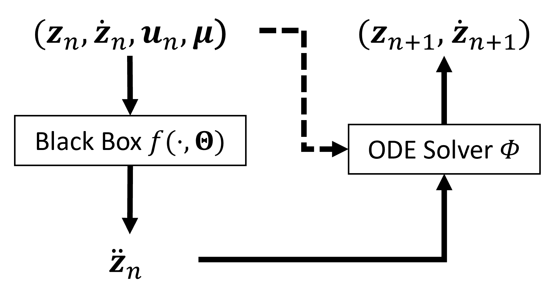

Figures 1 and 2 show the discretized version of the forward pass for the MBD with and without constraints. The constraint-related formulations are discussed in the Section 2.2.5. Within the MBD-NODE framework, the initial state of the system is processed using an ODE solver, evolving over a time span under the guidance of a neural network’s parameters. This neural network is trained to determine the optimal parameters that best describe the system’s dynamics. This continuous approach, in contrast to discrete-time models, often results in enhanced flexibility, efficiency, and good generalization accuracy. Based on the notation used for the definition of MBD-NODE in equation (6), we employ the corresponding three-layer neural network architecture in Table 1; the activation function can be Tanh and ReLU ActivationFC , and the initialization strategy used is that of Xavier xavier_ini , and Kaiming kaiming_ini .
| Layer | Number of Neurons | Activation Function | Initialization |
|---|---|---|---|
| Input Layer | [Tanh,ReLU] | [Xavier, Kaiming] | |
| Hidden Layer 1 | [Tanh,ReLU] | [Xavier, Kaiming] | |
| Hidden Layer 2 | [Tanh,ReLU] | [Xavier, Kaiming] | |
| Output Layer | - | [Xavier, Kaiming] |
2.2.4 Loss Function and Optimization without Constraints
First, we discuss the loss function for the MBD without constraints. Without loss of generality, we assume there are no additional parameters for notation simplicity. For a given initial state , assume the system’s next state is obtained with the integrator used over a time interval , which can be one or several numerical integration time steps. The loss function used for the MBD-NODE describes the mean square error (MSE) between the ground truth state and the predicted state:
| (14) |
where is the predicted state by integration with the derivatives from MBD-NODE.
For a trajectory of states , the common way Chen_NODE_2018 is to treat the first state as initial condition and all other states as targets, so the loss function could be defined as that:
| (15) |
The training phase is to refine the neural network’s parameters, ensuring that the predicted states mirror the true future states, which yields the optimization problem
| (16) |
Similar to most deep learning models, the parameter optimization of MBD-NODE can be conducted by backpropagation via stochastic gradient descent (SGD). The key for NODE-based frameworks is that the objective is to fit the entire trajectory, which necessitates the storage of intermediate gradients through the integration of the whole trajectory by backpropagation. This process needs a memory cost of , where represents the number of time steps of the trajectory, is the number of neural network calls per integration step, and is the number of layers in the NODE. To solve this, adjoint methods Chen_NODE_2018 and their adaptive enhancements adap_adjoint_NODE were implemented in the NODE-based model, achieving gradient approximation with only memory costs. Further, specialized adjoint methods have been proposed for symplectic integrators adjoint_symplectic and SONODE norcliffe2020secondNODE , each tailored for specific applications.
In practice, optimizing parameters to fit lengthy trajectories from highly nonlinear dynamics did not work well for our problems. To address this, we partition the long trajectory, consisting of states, into shorter sub-trajectories of length . The training process is then moved to these sub-trajectories. While this strategy makes the optimization easier, it may slightly impair the neural network’s capacity for long-term prediction. In practice, we set to be 1 for our numerical test, and we didn’t find the obvious loss of capacity for long-term prediction. In this case, the loss function will be the sum of the loss of each sub-trajectory:
| (17) |
The constant , the number of neural network calls per integration step, depends on the integrator used. For the Runge-Kutta 4th order method, the is 4 because we need to evaluate the acceleration at intermediate states during one step of integration, while for the Forward Euler method, is 1. Also, for the implicit solvers, is the same as their explicit version because, in the training stage, we already have the next state.
Given these considerations, the memory cost for optimization via backpropagation remains within acceptable limits. For the system subject to constraints (discussed in section 2.2.5), the adjoint method may not align with the used method. Upon reviewing recent literature, we found no instances of the adjoint methods being applied to constrained problems. Based on these, we finally choose backpropagation to optimize the neural network. The main process for training the MBD-NODE without constraints is summarized in the Algorithm 1 of Appendix A.
2.2.5 Loss Function and Optimization with Constraints
For MBD problems, accounting for constraints in the evolution of a system is imperative. These constraints capture not only physical design attributes, e.g. a spherical joint requires two points to coincide, but also factor in conservation laws, e.g., energy, numerical Hamiltonian. Accounting for these constraints is important in MBD. However, integrating constraints within deep neural network models is still an open problem, and further research and exploration are necessary.
From a high vantage point, constraints fall in one of two categories. Holonomic constraints depend solely on the coordinates without involving the latter’s time derivatives, and can be represented as . Nonholonomic constraints, involving the time derivatives of the coordinates and cannot be time-integrated into a holonomic constraint, are denoted as .
Additionally, constraints can be categorized based on their temporal dependency. Scleronomic constraints, or geometric constraints, do not explicitly depend on time and are expressed as . In contrast, rheonomic constraints, which depend on time, can also be framed in the form .
In summary, using the same notation in the above Section 2.2.4, the MBD constraints can be expressed in a generalized form , and the optimization problem solved can be posed as:
| (18) | ||||
| s.t. | (19) |
where is the areas from the prior physical knowledge that the MBD should have constraints.
There are two common ways to handle hard constraints. One is to relax this hard constrained problem to a soft constraint problem by adding the constraints to the loss function as a penalty term fortin2000augmented ; PINN_constraints ; lim2022unifying ; PINODE_constraints-djeumou22a . The loss function then becomes
| (20) |
where represents the function for the -th constraint, typically comprising a quadratic and a linear term, as is common in the well-known augmented Lagrangian method fortin2000augmented ; PINODE_constraints-djeumou22a ; PINN_constraints . The primary advantage of this approach is its ease of implementation, requiring only the addition of constraints as a regularization term. However, there are several drawbacks to it: the optimization process may not always converge, and the use of regularization can often diminish accuracy. Most critically, the constraints are applied exclusively within the training set’s phase space, rendering them ineffective in domains beyond this phase space.
The alternative is to enforce the constraints in both the training and inference stages without adding a constraint loss term. Based on a coordinates partition technique Wehage82 , we denote the minimal (or independent) coordinates as and the dependent coordinates as . Then, the dependent coordinates can be obtained from the independent coordinates and the prior knowledge of constraints:
| (21) |
where is defined as the inverse function that maps the value of minimal coordinates to the dependent coordinates, and typically does not have a closed form yet it can be evaluated given . If the MBD system has generalized coordinates and position constraints ( DOF), we build the MBD-NODE only with the minimal coordinates . Depending on whether we have the ground truth data of the dependent coordinates , the training stage could be divided into two cases:
(1) If we have the complete information of the dependent coordinates , we can first input minimal state to get the acceleration for integration to get the minimal state at the next time step . Then, we can solve the dependent state by solving the constraint equation . We could use the minimal coordinates and dependent state to get the full combined states . By the difference between the combined predicted state and the ground truth state , we can optimize the MBD-NODE. A similar concept has been explored in beucler2021enforcing ; daems2022keycld for enforcing hard constraints within data-driven models. Beucler et al. beucler2021enforcing have approached this by designing a constraint layer, while Daems et al. daems2022keycld encoded holonomic constraints directly into the Euler-Lagrange equations. Our method can address more general non-holonomic constraints. Given the initial state and the ground truth state , the corresponding loss function for one data pair could be written as:
| (22) | ||||
(2) If we have access to only the minimal state information —for instance, if we prefer not to expend effort in collecting data on dependent coordinates due to potential costs—we can construct and train the MBD-NODE using solely the minimal coordinates . During the inference, we could use MBD-NODE to predict minimal states and then solve all the states. In this case, the loss function could be written as:
| (23) |
By solving the constraint equation in both the training (with dependent coordinates data) and inference stage, the hard constraints are satisfied in both phases. The algorithm for constraints equation-based optimization is summarized in the Algorithm 2 (which utilizes dependent coordinates data) and Algorithm 3 (which uses only minimal coordinates data), both found in Appendix A.
2.2.6 Baseline Models
Table 2 summarizes the models used in the numerical tests discussed in this manuscript, along with some of their salient attributes. Code for all of these methods is provided with this contribution.
| MBD-NODE | HNN | LNN | LSTM | FCNN | |
|---|---|---|---|---|---|
| Works on energy-conserving system | ✓ | ✓ | ✓ | ||
| Works on general coordinates | ✓ | ✓ | ✓ | ✓ | |
| Works on dissipative systems | ✓ | ✓ | ✓ | ||
| Works with constraints | ✓ | ||||
| No need for second-order derivatives | ✓ | ✓ | |||
| Scalability for long time simulation | ✓ | ✓ | ✓ | ||
| Learn continuous dynamics | ✓ | ✓ | ✓ | ✓ |
3 Numerical Experiments
We study the performance of the methods in Table 2 with seven numerical examples, reflecting on method attributes such as energy conservation, energy dissipation, multi-scale dynamics, generalization to different parameters and external force, model-based control, chaotic dynamics, and constraint enforcement. One or more of these attributes oftentimes comes into play in engineering applications that rely on MBD simulation. We use these numerical examples to compare the performance of the proposed MBD-NODE methodology with state-of-the-art data-driven modeling methods. The numerical examples and modeling methods are summarized in Table 3.
| Test Case | Model A | Model B | Model C |
|---|---|---|---|
| Single Mass-Spring | MBD-NODE | HNN | LNN |
| Single Mass-Spring-Damper | MBD-NODE | LSTM | FCNN |
| Triple Mass-Spring-Damper | MBD-NODE | LSTM | FCNN |
| Single Pendulum | MBD-NODE | LSTM | FCNN |
| Double Pendulum | MBD-NODE | LSTM | FCNN |
| Cart-pole | MBD-NODE | LSTM | FCNN |
| Slider Crank | MBD-NODE | - | - |
The model performance is evaluated via the MSE , defined by the following equation:
| (24) |
where indicates the index of a test sample, and are the ground truth of the coordinate and its time derivative, while and denote the predicted results by a trained model. Here corresponds to the standard vector 2-norm.
In Table 4, we summarize the MSE error made by each method on the test data of all the numerical examples. Sections 3.1 to 3.7 present more details about the setup of each test case and the performance of our method in comparison to the others. The training cost for the MBD-NODE, HNN, LNN, LSTM, and FCNN models with different integrators used for each test case is recorded in the Appendix B. Python code is provided publicly for all models and all test cases for unfetter used and reproducibility studies MNODE_supportData2024 .
| Test Case | Error | ||
|---|---|---|---|
| Model A | Model B | Model C | |
| Single Mass-Spring | 1.3e-6 | 1.9e-2 | 9.1e-6 |
| Single Mass-Spring-Damper | 8.6e-4 | 1.8e-2 | 9.9e-2 |
| Triple Mass-Spring-Damper | 8.2e-3 | 1.8e-1 | 4.2e-2 |
| Single Pendulum | 2.0e-3 | 3.4e-3 | 8.0e-1 |
| Double Pendulum | 2.0e-1 | 6.4e-1 | 2.2e0 |
| Cart-pole | 6.0e-5 | 3.2e-4 | 4.7e-2 |
| Slider Crank | 3.2e-2 | - | - |
3.1 Single Mass-Spring System
This system is relevant as it does not model viscous damping and serves as a numerical example to evaluate the predictive attribute of the trained models on an energy-conserving system HNN ; HNN_IET ; NSF_HNN . Figure 3 illustrates the setup of the single mass-spring system. The equation of motion is formulated as
| (25) |
where represents the displacement of the mass from its equilibrium position; , the spring constant, is set to 50 N/m; and , the mass of the object, is set to 10 kg. The system’s Hamiltonian, which describes its total energy, is
| (26) | ||||
| (27) | ||||
| (28) |
where: is the generalized position; is the generalized momentum, which, in this context, is , with being the generalized velocity; and and represents the kinetic energy and potential energy.
We choose a time step of 0.01s in both training and testing for the single mass-spring system. The training data consists of a trajectory analytically solved over 300 time steps with initial conditions .
For this system, which possesses a separable Hamiltonian as shown in Eq. (28), the MBD-NODE model employed the leapfrog method as the symplectic integrator of choice. We also show the performance of MBD-NODE when used with the more common RK4 integrator. We also benchmark against the HNN and LNN methods (see Table 3 for a summary). The Hamiltonian-based methods used data in generalized coordinates, while the others (including a numerical method) were tested using Cartesian coordinates. We also provide a baseline test by numerically solving the system of ODEs in Eq. (25) with the RK4 integrator. The specific configurations of each model, including the choice of coordinate systems and integrators, are detailed in Table 5. Additionally, the hyperparameters used for the neural network-based tests are summarized in Table 6. These settings and tests were designed to evaluate the efficiency and accuracy of different modeling approaches and integrators in predicting and understanding the dynamics of the single mass-spring system.
| Model | Coordinate System | Integrator | MSE |
|---|---|---|---|
| MBD-NODE | Generalized | Leapfrog | 1.3e-6 |
| HNN | Generalized | RK4 | 2.0e-3 |
| LNN | Cartesian | RK4 | 9.1e-6 |
| Numerical | Cartesian | RK4 | 2.0e-3 |
| MBD-NODE | Cartesian | RK4 | 9.2e-1 |
| Hyper-parameters | Model | |||
|---|---|---|---|---|
| MBD-NODELF | MBD-NODERK4 | HNN | LNN | |
| No. of hidden layers | 2 | 2 | 2 | 2 |
| No. of nodes per hidden layer | 256 | 256 | 256 | 256 |
| Max. epochs | 450 | 300 | 30000 | 400 |
| Initial learning rate | 1e-3 | 1e-3 | 1e-3 | 1e-4 |
| Learning rate decay | 0.99 | 0.98 | 0.98 | 0.98 |
| Activation function | Tanh | Tanh | Sigmoid,Tanh | Softmax |
| Loss function | MSE | MSE | MSE | MSE |
| Optimizer | Adam | Adam | Adam | Adam |
Figure 4 shows the dynamic response in terms of position and velocity for the test data, and the MSE of each method is shown in Table 5. More specifically, Figs. 4 (a) to (d) demonstrate the performance of the MBD-NODE model with the RK4 integrator, as well as the results obtained from a purely numerical solution using the RK4 method. The ground truth for comparison is obtained by analytically solving Eq. (25). It can be seen in Figs. 4 (c) and (d) that the direct usage of the RK4 integrator provides results that gradually deviate from the true system. This issue of gradually increased errors becomes more severe in the MBD-NODE results with the RK4 integrator in Figs. 4 (a) and (b), highlighting their limitations in accurately modeling Hamiltonian systems. In contrast, both the LNN and HNN models, despite utilizing the RK4 integrator, demonstrate stable behavior in solving the mass-spring system, as shown in Figs. 4 (g) to (j). The more stable simulations of these two models can be attributed to the underlying equations of these models, which ensure energy conservation in the system. Notably, the HNN’s performance, as shown in Figs. 4(i) and (j), show a deviation from the expected trajectory around the 30-second mark, leading to a higher MSE when compared to the MBD-NODE with the leapfrog integrator and the LNN model. Among all the methods that we studied, the MBD-NODE with the leapfrog integrator outperforms other models, achieving the lowest MSE of =1.3e-6, with detailed trajectories of and presented in Figs. 4(e) and (f).
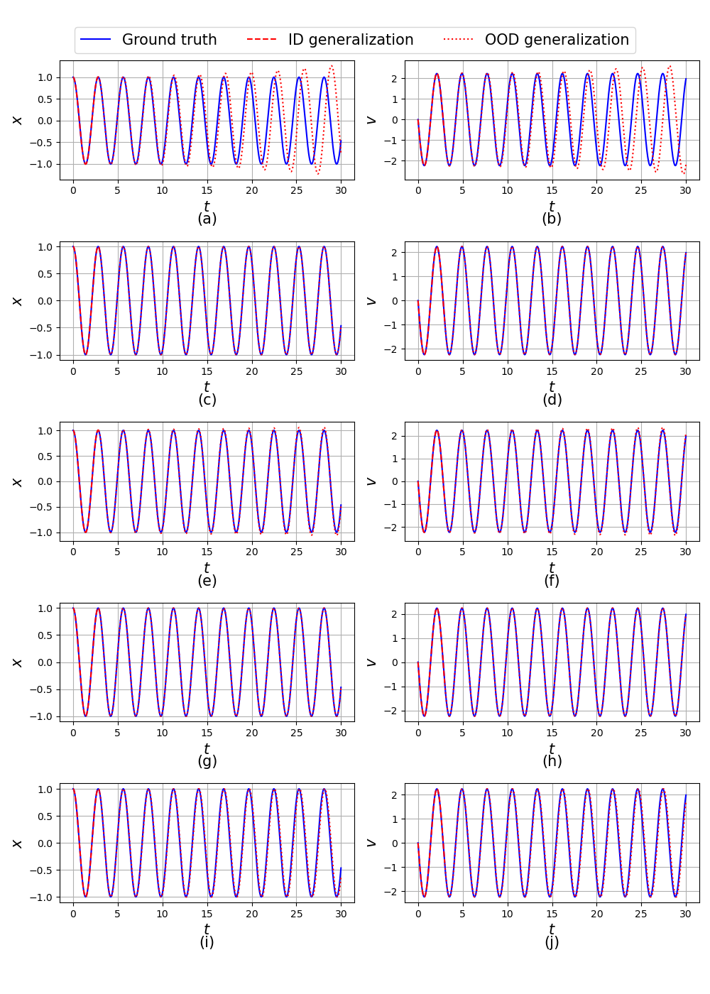
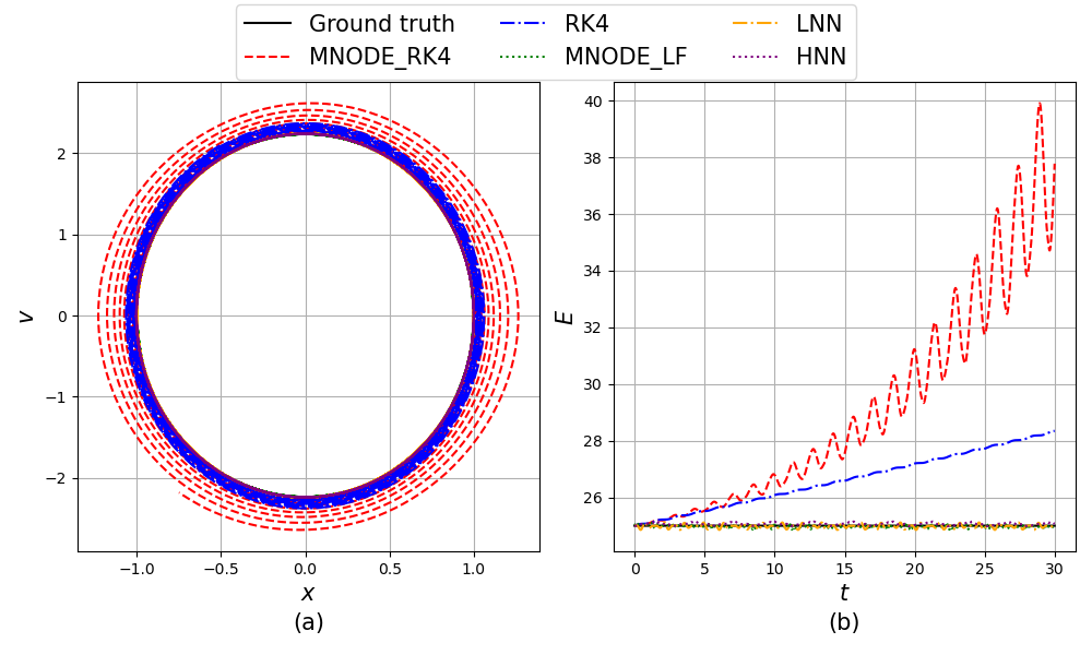
Figure 5 presents the phase space trajectory and energy profile for the test set. It confirms the instability issues with the RK4 solver and the MBD-NODE model with the RK4 integrator, particularly in terms of energy drift accumulating over time. In comparison, both the LNN and HNN models, as well as the MBD-NODE model with the leapfrog integrator, demonstrate stable solutions without any noticeable energy drift. The results in Figs. 4 and 5 confirm the effectiveness of the MBD-NODE model with a symplectic integrator in accurately learning the Hamiltonian structure of the system.
3.2 Single Mass-Spring-Damper System
The second numerical test involves a single-mass-spring-damper system, as shown in Fig. 6. Compared with the first numerical test, there is a damper between the mass and the wall that causes the mass to slow down over time. It is important to note that the models designed for energy-conserving systems, like the LNN and HNN, are generally not applicable for dissipative systems without further modification. Therefore, we compare the performance of our method to LSTM and FCNN models, which are commonly employed in multibody dynamics problems.
The equation of motion for the single-mass-spring-damper system is given by:
| (29) |
where represents the displacement of the mass from its equilibrium position; is the mass of the object, set to 10 in this test; is the damping coefficient, set to in this test; and is the coefficient of stiffness of the spring, set to .
We choose the time step as 0.01s for both the training and testing. The training dataset consists of a trajectory numerically solved by the RK4 solver for 300 time steps. In the testing phase, the models are tested by predicting the system state within the training range and extrapolation to predict system behavior for an additional 100 time steps. The initial condition for this problem is . It should be noted that the system is no longer a Hamiltonian system, so we use Cartesian coordinates for all the methods. The hyperparameters used for each model are summarized in Table 7.
| Hyper-parameters | Model | ||
|---|---|---|---|
| MBD-NODE | LSTM | FCNN | |
| No. of hidden layers | 2 | 2 | 2 |
| No. of nodes per hidden layer | 256 | 256 | 256 |
| Max. epochs | 350 | 400 | 600 |
| Initial learning rate | 1e-3 | 5e-4 | 5e-4 |
| Learning rate decay | 0.98 | 0.98 | 0.98 |
| Activation function | Tanh | Sigmoid,Tanh | Tanh |
| Loss function | MSE | MSE | MSE |
| Optimizer | Adam | Adam | Adam |
Figure 7 presents the position and velocity for all the trained models. In the first 300 time steps, which correspond to the training range, all three models exhibit accurate predictions, indicating an effective training process. However, differences in model performance start to show up in the testing regime (i.e., ). More specifically, Fig. 7(a) and (b) show that the MBD-NODE gives a reasonable prediction that closely matches the ground truth with the lowest MSE of 8.6e-4, which demonstrates its predictive capability.
On the other hand, the LSTM predictions tend to just replicate historical data patterns (see Fig. 7(c) and (d)), rather than learning and adapting to the underlying dynamics of the system. This limitation makes LSTM fail to correctly capture the decay of energy for an energy-dissipative system. The FCNN model struggles with extrapolation as well, mainly because the good extrapolation performance of FCNN heavily relies on the closeness of training and testing data in their distributions. This limitation of FCNN leads to errors in the extrapolation task of this example, resulting in the largest MSE of as shown in Fig. 7(e) and (f).
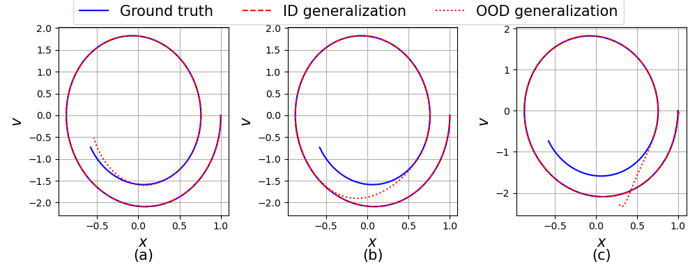
More insights into the system’s dynamics are provided by the phase space trajectories illustrated in Fig. 8. The predictions of the MBD-NODE, as depicted in Fig. 8(a), are closely aligned with the observed behavior of the system. In contrast, the LSTM’s trajectory, shown in Fig. 8(b), exhibits stagnation and fails to reflect the system’s eventual halt. The FCNN’s performance, presented in Fig. 8(c), is lacking during the extrapolation test – it merely yields predictions in the tangent direction, resulting in a significant divergence from the anticipated trajectory.
3.3 Multiscale Triple Mass-Spring-Damper System
This system, shown in Fig. 9, has three masses. The largest mass is 100 times larger than the smallest one. The main purpose of this example is to gauge method performance on multiscale systems. The equations of motion for the triple mass-spring-damper system are as follows:
| (30) | ||||
where are the positions of the masses, respectively; are the masses of the object with values of 100 kg, 10 kg, and 1 kg, respectively; are the damping coefficients, each set to 2 Ns/m; and are the spring stiffness values, all set to 50 N/m.
For the numerical settings of the triple mass-spring-damper system, we choose the time step as 0.01s for both training and testing. The training dataset has a trajectory numerically computed by the RK4 solver for 300 time steps. The initial conditions are set as (all units are SI). The models are tested by extrapolating for 100 more time steps. The hyperparameters used for the models are summarized in Table 8.
| Hyper-parameters | Model | ||
|---|---|---|---|
| MBD-NODE | LSTM | FCNN | |
| No. of hidden layers | 2 | 2 | 2 |
| No. of nodes per hidden layer | 256 | 256 | 256 |
| Max. epochs | 350 | 400 | 600 |
| Initial learning rate | 6e-4 | 5e-4 | 5e-4 |
| Learning rate decay | 0.98 | 0.98 | 0.98 |
| Activation function | Tanh | Sigmoid,Tanh | Tanh |
| Loss function | MSE | MSE | MSE |
| Optimizer | Adam | Adam | Adam |
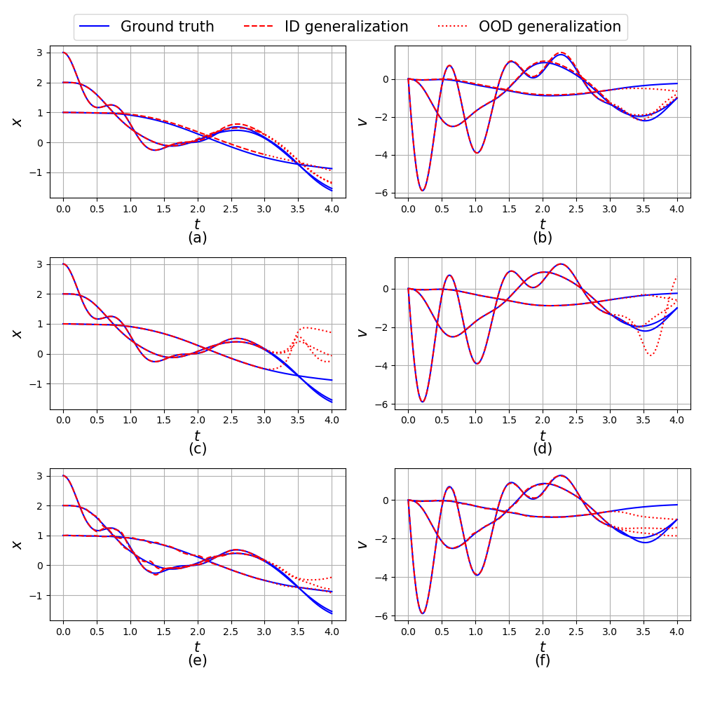
Figure 10 presents the position and velocity of the triple mass-spring-damper system during training and testing. In terms of accuracy, the MBD-NODE outperforms other models with an MSE = 8.2e-3. More specifically, the MBD-NODE and LSTM models provide accurate results in the range of training data (i.e., ) while the results of FCNN model show small oscillation mainly due to the multiscale setting of the dynamics shown in Fig. 10(e). In the testing data (i.e., ), the performance of trained models starts to differ more. The MBD-NODE can still give a reasonable prediction for the triple mass-spring-damper system shown in Fig. 10(a) and (b), although the predicted trajectories slowly deviate from the true ones, mainly because of the accumulation of numerical errors. On the other hand, the LSTM tends to replicate some of the historical patterns. The testing performance of the FCNN model is more reasonable than the LSTM model in this example, while still less satisfactory compared with the MBD-NODE model.
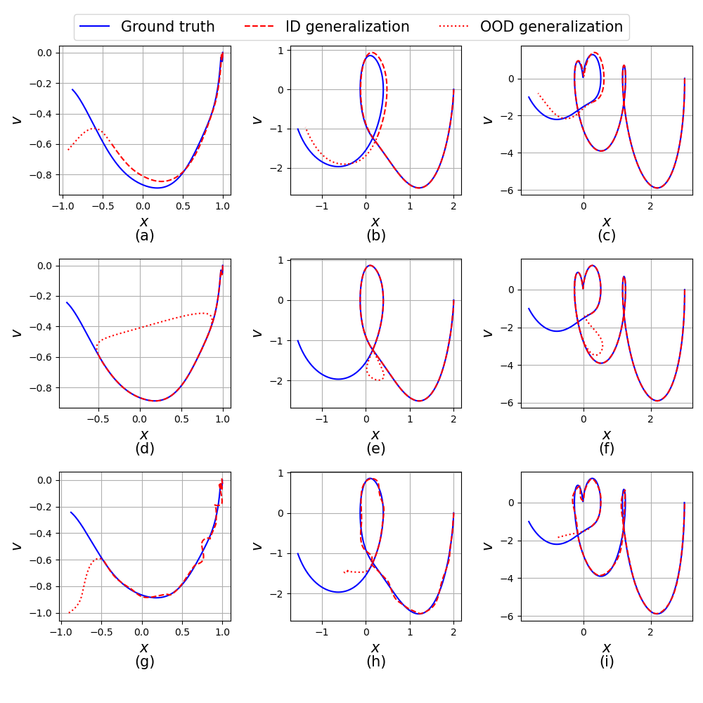
The trajectory for the triple mass spring damper system for the test set is shown in Fig. 11. We can see that for the MBD-NODE, the trajectory of the first body shown in Fig. 11(a) has some mismatch with the ground truth. This is caused by the multiscale property that the first mass has the largest mass which leads to the slightest change in the position and velocity , while the MBD-NODE learns the dynamics from the difference between the state at two nearby times. So, the largest mass will contribute the least to the loss, which causes the MBD-NODE to learn the dynamics of the first body inadequately. The numerical integration error also accumulates during the inference, which makes the error larger. For LSTM, we can more clearly see its prediction trends converge to the historical data, which does not work well during OOD generalization. For FCNN, we note the oscillation for the first body in ID generalization, and for the OOD generalization, which leads to a lackluster predictive performance.
3.4 Damped Single Pendulum
In this section, we test the MBD-NODE’s ability to generalization on different initial conditions and external forces using the damped single pendulum as shown in Fig. 12. The equation of motion Eq. (31) for a damped single pendulum, including the gravitational and damping forces, can be represented as a second-order ODE as follows:
| (31) |
where is the angular displacement as a function of time, is the acceleration due to gravity and external force, m is the length of the pendulum, Ns/m is the damping coefficient, and kg is the mass of the pendulum bob.
Initially, we examine a scenario where the pendulum is released from its lowest point with an initial angular velocity of . We employ various models to predict the trajectory of the pendulum using identical training and testing datasets. In practice, the midpoint method is utilized to solve the ODE Eq. (31), adopting a time step of 0.01 seconds. The dataset for training spans the initial 3 seconds, whereas the testing dataset covers the subsequent 1 second. The hyperparameters applied across the models are detailed in Table 9.
| Hyper-parameters | Model | ||
|---|---|---|---|
| MBD-NODE | LSTM | FCNN | |
| No. of layers | 2 | 2 | 2 |
| No. of nodes per hidden layer | 256 | 256 | 256 |
| Max. epochs | 400 | 400 | 600 |
| Initial learning rate | 6e-4 | 5e-4 | 5e-4 |
| Learning rate decay | 0.98 | 0.98 | 0.98 |
| Activation function | Tanh | Sigmoid,Tanh | Tanh |
| Loss function | MSE | MSE | MSE |
| Optimizer | Adam | Adam | Adam |
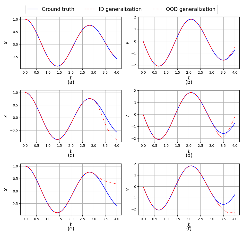
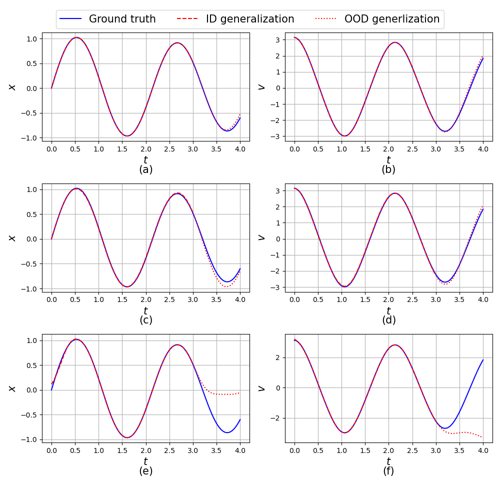
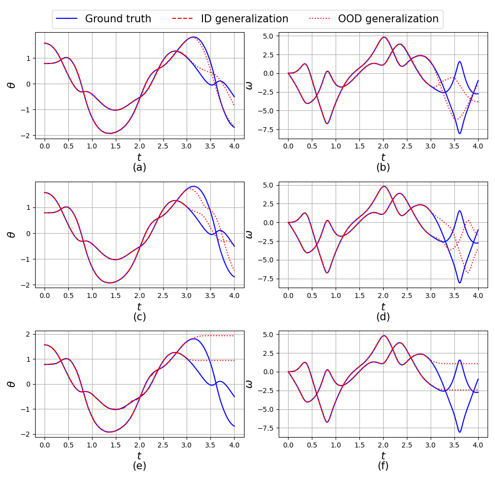
Figures 13 and 14 present the dynamics response and the phase space of the single pendulum system during the ID generalization and OOD generalization. The MBD-NODE outperforms other models with an MSE = 2.0e-3. Although LSTM has a small MSE = 3.4e-3, it tends to replicate some of the historical patterns and fails to capture the damping effect for OOD generalization. The FCNN model has a larger MSE = 8.0e-1, associated with the lackluster OOD generalization ability of the FCNN model.
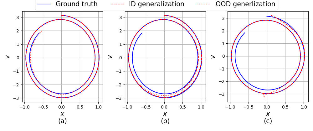
Beyond the first setting, we test MBD-NODE’s ability to generalize under varying initial conditions and external forces. Importantly, we use the MBD-NODE trained in the first setting directly without adding new training data – a significant challenge for OOD generalization. FCNNs and LSTMs are not suitable for handling time-varying external forces. They can only work with different parameters that do not change with respect to time. For FCNNs, accommodating changes in initial conditions would require a larger model, additional data, and retraining. Therefore, we only test MBD-NODE in this setting. Additionally, MBD-NODE’s nature allows us to directly calculate acceleration from external forces and incorporate it, simplifying integration with gravity as shown in Fig. 2.
Figure 15 presents the dynamics response of the single pendulum system with four different unseen initial conditions given in four quadrants. Because the MBD-NODE learns the dynamics related to the range of the phase space covered in the training set and does so independently of the initial condition, MBD-NODE yields a reasonable prediction for any of the four different initial conditions.
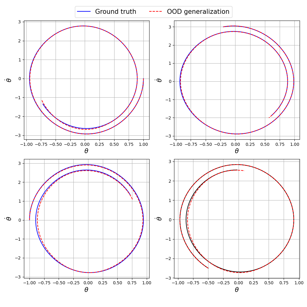
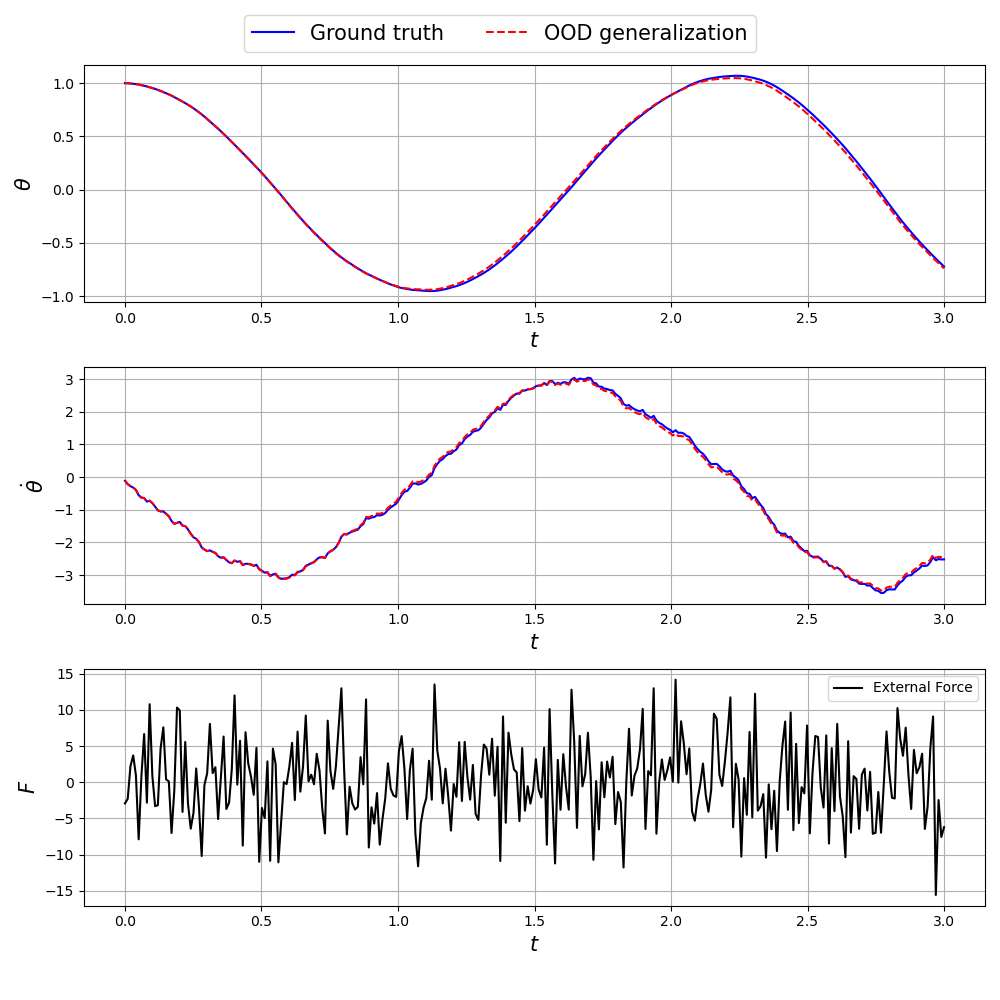
Figure 16 presents the dynamics response of the single pendulum system with random external force. Here, we sample the external force from the normal distribution and apply it to the single pendulum at every time step. We predict 300 time steps for the single pendulum with random excitation. Because the force will push the pendulum to unseen state space, this is a good test to probe the MBD-NODE’s OOD generalization ability. MBD-NODE can continue to give an accurate prediction for the single pendulum system under random external force.
3.5 Double Pendulum
To gauge the performance of our model on chaotic systems, we study the double pendulum system (see Fig. 17) as a numerical example. This pendulum system has two masses and , lengths and , and two angles and . The generalized momenta corresponding to these angles are and , which needs to be calculated by using the Lagrangian. The Hamiltonian for this system is given by:
| (32) |
where is the kinetic energy and is the potential energy. For the double pendulum system, the kinetic energy and potential energy are given by:
| (33) | ||||
| (34) |
The Hamiltonian can be expressed in terms of and as:
| (35) | ||||
The gradients of the Hamiltonian, and , can be used to derive the Hamilton’s equations of motion:
| (36) | ||||
| (37) |
The specific Hamilton’s equations of motion for the double pendulum system are:
| (38) | ||||
| (39) | ||||
| (40) | ||||
| (41) |
where:
| (42) | ||||
| (43) |
The double pendulum system is defined as follows: rod lengths, m; concentrated masses, kg; gravitational acceleration, m/s2; initial angular displacement of the first mass, ; initial angular velocity of the first mass, ; initial angular displacement of the second mass ; initial angular velocity of the second mass . We set the time step as 0.01s for both training and testing. The training dataset has a trajectory numerically computed via RK4 for 300 time steps. The models are tested by extrapolating for 100 more time steps. The hyperparameters used for the models are summarized in Table 10.
| Hyper-parameters | Model | ||
|---|---|---|---|
| MBD-NODE | LSTM | FCNN | |
| No. of hidden layers | 2 | 2 | 2 |
| No. of nodes per hidden layer | 256 | 256 | 256 |
| Max. epochs | 450 | 400 | 600 |
| Initial learning rate | 1e-3 | 5e-4 | 5e-4 |
| Learning rate decay | 0.98 | 0.98 | 0.99 |
| Activation function | Tanh | Sigmoid,Tanh | Tanh |
| Loss function | MSE | MSE | MSE |
| Optimizer | Adam | Adam | Adam |
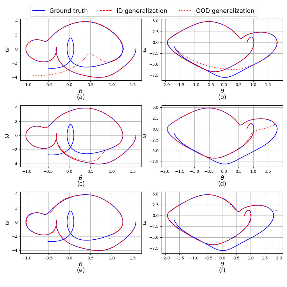
Figure 18 shows the dynamic response of the different methods for a double pendulum. We can observe that all three models can give good predictions in the range of the training set. In the extrapolation range, the three models gradually diverge. The challenge for integrator-based methods like MBD-NODE is particularly pronounced due to the inherently chaotic nature of the double pendulum system, which tends to amplify integration errors rapidly, leading to significant discrepancies. For a discussion about the limitations of numerical integration methods like the Runge-Kutta and integration-based neural networks like Physics-Informed Neural Networks (PINN), the reader is referred to PINN_cheats . For the double pendulum problem, these two approaches give large divergence for small initial perturbation. Despite this, the MBD-NODE outperforms the two other models with an MSE of 2.0e-1.
The phase space trajectories obtained by the three models are shown in Fig. 19. We can observe that the MBD-NODE model overall outperforms the other two models in the testing data regime. Although there are noticeable differences between the prediction and ground truth for the MBD-NODE model, it’s still trying to capture the patterns of ground truth in the testing regime, especially for the second mass. On the contrary, the LSTM model tends to replicate the historical trajectories as shown in Fig. 19(c) and (d). For example, the FCNN fails to demonstrate predictive attributes outside of the training regime.
3.6 Cart-pole System
In this section, we consider the cart-pole system, which is a classical benchmark problem in control theory. As shown in Fig. 20, the system consists of a cart that can move horizontally along a frictionless track and a pendulum that is attached to the cart. The pendulum is free to rotate about its pivot point. The system’s state is described by the position of the cart , the velocity of the cart , the angle of the pendulum , and the angular velocity of the pendulum . The equations of motion for the cart-pole system are given by the following second-order nonlinear ODEs:
| (44) | ||||
where is the mass of the cart and is the mass of the pole, is the length of the pole, and is the external force horizontally applied to the cart with unit .
We first consider the case in which the cart-pole system is set to an initial position, and then we let the system evolve without any external force being applied. The initial conditions are set as follows:
| (45) |
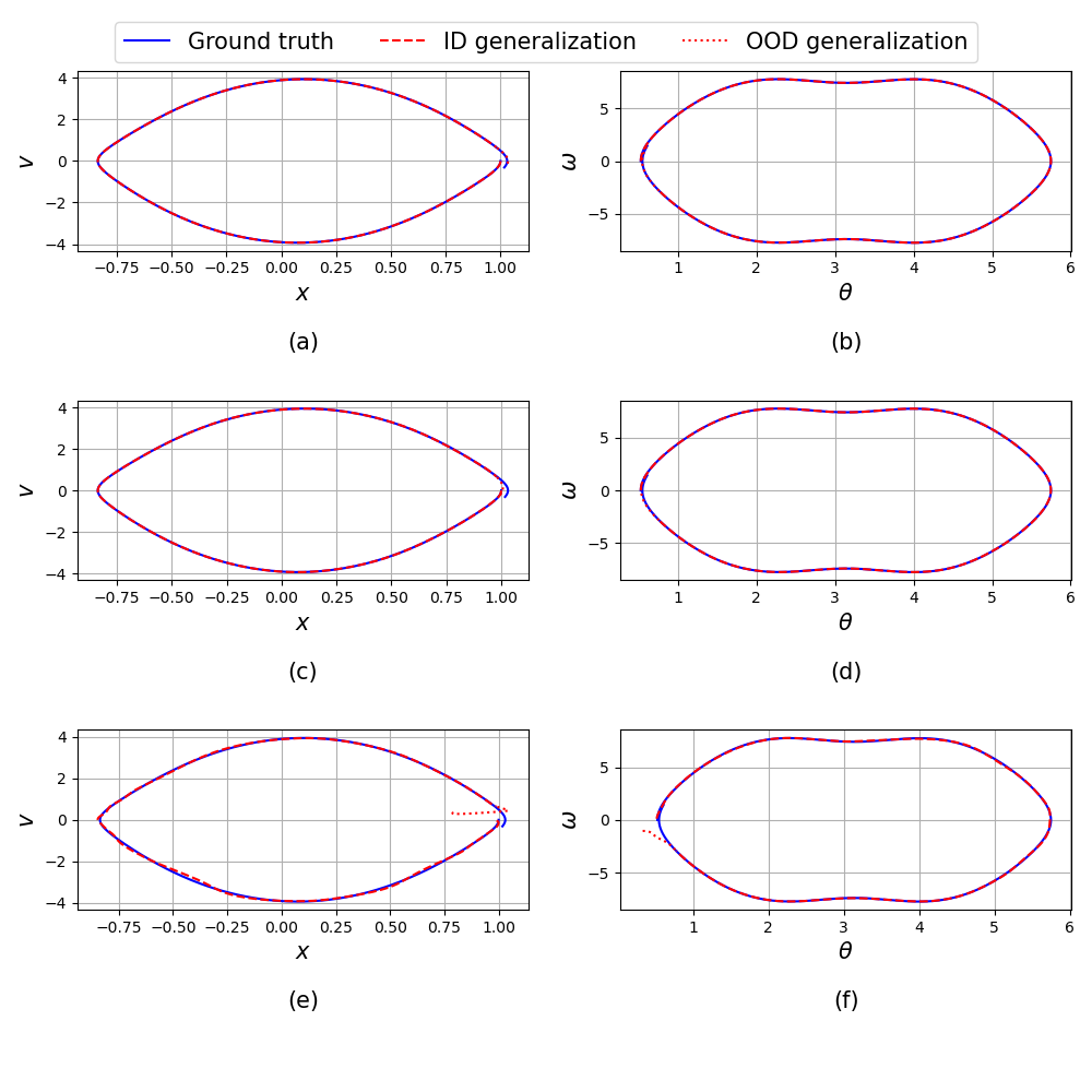
The system is simulated using the midpoint method with a time step of 0.005s. We generate the training data by simulating the system for 400 time steps and the testing data by simulating the system for 100 time steps. As shown in Figs. 21 and 22, the MBD-NODE can accurately predict the system dynamics with . Because this case is a periodic system that time series data can fully describe, the LSTM model can also provide accurate predictions with . However, the FCNN model still gives lackluster OOD generalization performance with . The hyperparameters for each model are summarized in Table 11.
| Hyper-parameters | Model | ||
|---|---|---|---|
| MBD-NODE | LSTM | FCNN | |
| No. of hidden layers | 2 | 2 | 2 |
| No. of nodes per hidden layer | 256 | 256 | 256 |
| Max. epochs | 450 | 400 | 600 |
| Initial learning rate | 1e-3 | 5e-4 | 5e-4 |
| Learning rate decay | 0.98 | 0.98 | 0.99 |
| Activation function | Tanh | Sigmoid,Tanh | Tanh |
| Loss function | MSE | MSE | MSE |
| Optimizer | Adam | Adam | Adam |
Furthermore, we consider the case that the cart-pole system is set to the initial position Eq. (45), and then we apply the external force to the cart to balance the pole and keep the cart-pole system at the origin point. In general control theory, model predictive control (MPC) is a popular method for solving this kind of control problem by linearizing the nonlinear system dynamics and solving a quadratic convex optimization problem over a finite time horizon at each time step. Specifically, for a linearized system dynamics , the optimization problem can be formulated as a convex optimization problem as follows kouvaritakis2016MPC :
| (46) | ||||
| s.t. | (47) | |||
| (48) |
where is the state of the system at time step , is the time horizon for optimization, is the control input at time step , and are the weighting matrices, which are set to the identity matrix, and and are the constraints for the state and control input, respectively.
For the cart-pole system, the matrix and can be easily derived from the system dynamics Eq. 44 by the first-order Taylor series approximation, which are:
| (49) |
As a high-accuracy and differentiable model, the MBD-NODE can be used to directly linearize the system dynamics by calculating the Jacobian matrix of the well-trained MBD-NODE. In this case, MBD-NODE captures the system dynamics by learning the map to the angular acceleration and the acceleration . In practice, the Jacobian matrix can be calculated by automatic differentiation, which is used to replace the matrix and in the MPC optimization problem. To get the well-trained MBD-NODE, we train the model with uniformly sampling data points in the range of for the state space and the control input. We limit our analysis to the MBD-NODE model as FCNN and LSTM models cannot work with time-evolving external input.
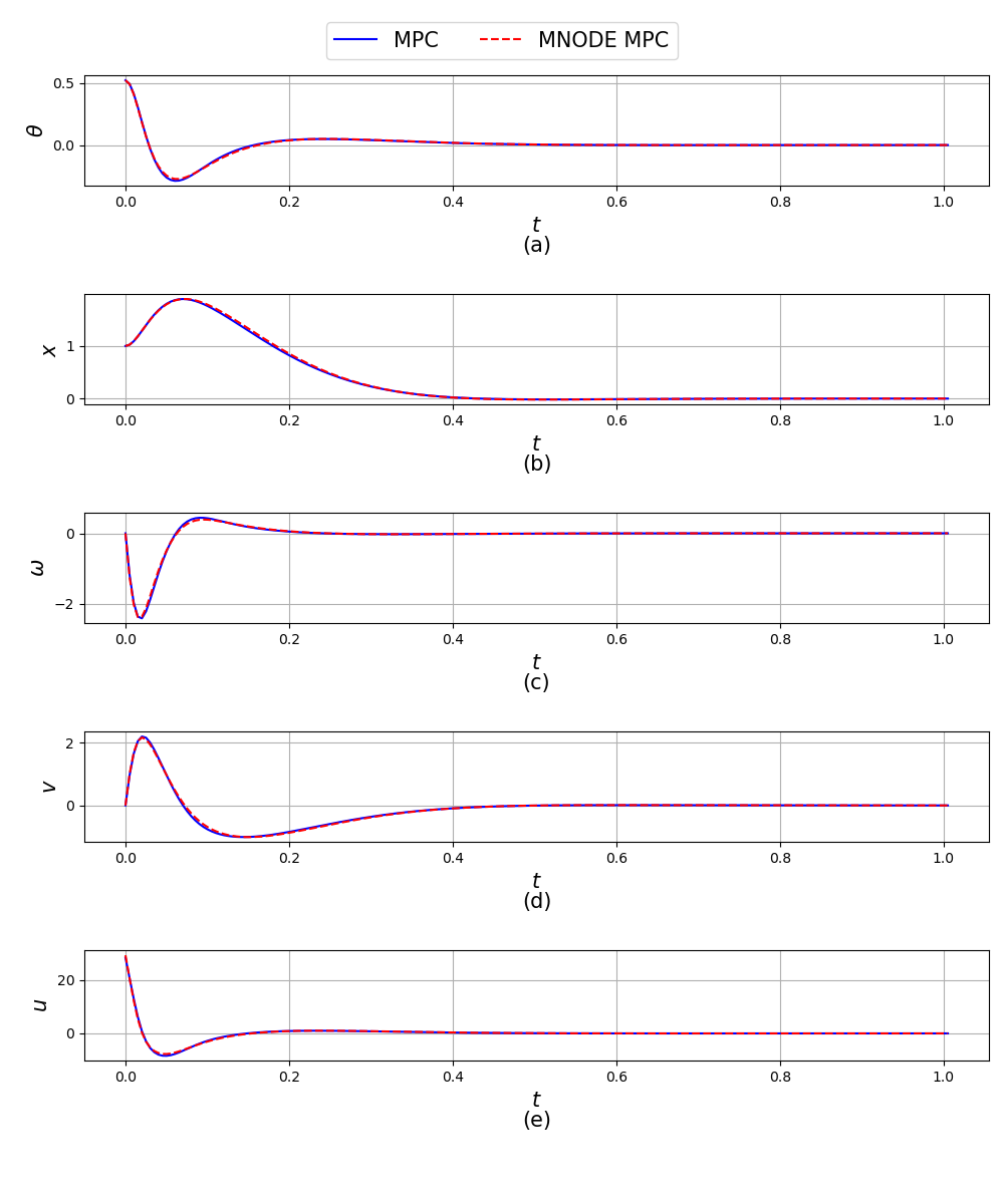
Figure 23 shows the trajectories and the obtained control input for the MPC methods and the MBD-NODE-based MPC method. We can see that the MBD-NODE-based MPC can provide high-accuracy control input and trajectory as the analytic equation of motion-based MPC, which also shows MBD-NODE’s strong ability to capture the system dynamics.
3.7 Slider-Crank Mechanism
We assessed MBD-NODE’s capacity for long-term, high-accuracy predictions using the slider-crank mechanism (Fig. 24). The test involved generating predictions for up to 10,000 time steps (100s), while encompassing generalization to arbitrary external forces and torques applied to both the slider and crank. We did not include LSTM and FCNN models in the comparison as their inherent structure does not readily accommodate the representation of system dynamics with variable external forces and torques. Additionally, LSTM and FCNN models face challenges in long-term prediction. Their training data requirements and computational costs scale linearly with the time horizon, whereas MBD-NODE’s performance depends on the phase space and external inputs, not directly on the time horizon. Previous FCNN- and LSTM-based approaches in related work HAN_DNN2021113480 ; Choi_DDSdd57a6f7c2064450bc1f79231ef67414 ; YE_MBSNET2021107716 ; efficient_PCA typically demonstrate short-term prediction capabilities, limited to durations of several seconds or hundreds of time steps.
We formulate the slider-crank mechanism as a three-body problem with hard constraints as follows:
-
1.
The crank is connected to ground with a revolute joint with mass , moment of inertia . The center of mass of the crank in the global reference frame is , and the length of the crank is .
-
2.
The rod is connected to the crank with a revolute joint with mass , moment of inertia . The center of mass of the rod in the global reference frame is expressed as , and the length of the connecting rod is .
-
3.
The slider is connected to the rod with a revolute joint and constrained to move horizontally with mass , moment of inertia . The center of mass of the slider in the global reference frame is .
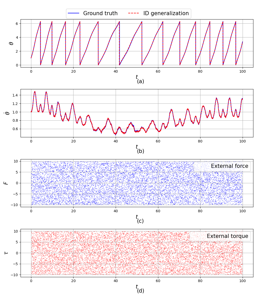
The generalized coordinate are used to describe the system dynamics. Given at a point in time , and some values of the external force/torque , we seek to produce the generalized acceleration ; i.e., we have a total of system states and external inputs to describe the system dynamics. Because the slider-crank mechanism is a one-DOF system, we take the minimum coordinates as with the external input ; these four variables fully determine the system dynamics. All other coordinates are treated as dependent coordinates. The detailed formulation is shown in the Appendix C.
For the training part, we uniformly sampled data points as providing the training data. The training used the hyperparameters shown in Table 12. In the testing part, we set the initial condition to be , the simulation time step as 0.01s and the external force and torque sampled from uniform distribution are applied to the system for each time step; note that there is no requirement for smoothness in and , although if one is present that would only help. We run the prediction for 10000 steps (100s) to test the MBD-NODE’s long-time prediction ability.
| Hyper-parameters | Model | ||
|---|---|---|---|
| MBD-NODE | LSTM | FCNN | |
| No. of hidden layers | 2 | - | - |
| No. of nodes per hidden layer | 256 | - | - |
| Max. epochs | 500 | - | - |
| Initial learning rate | 1e-3 | - | - |
| Learning rate decay | 0.98 | - | - |
| Activation function | Tanh | - | - |
| Loss function | MSE | - | - |
| Optimizer | Adam | - | - |
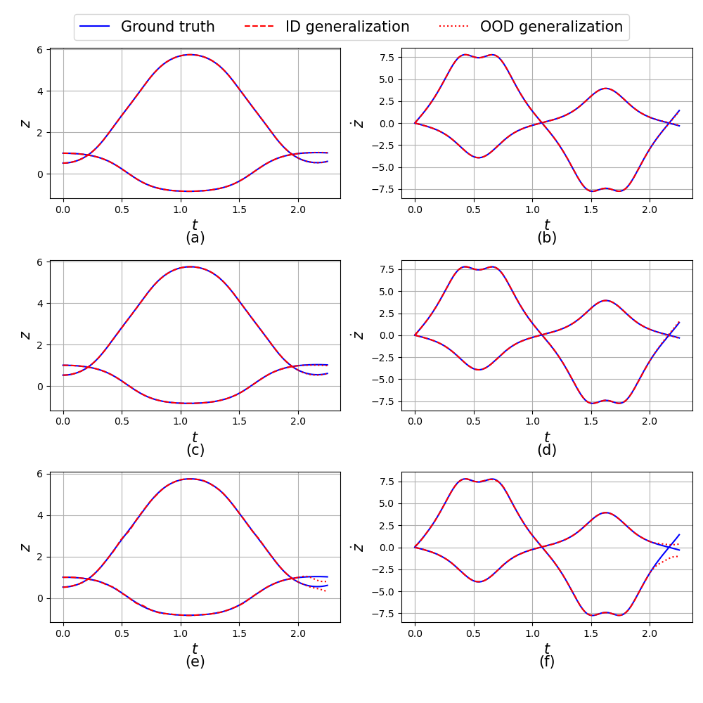
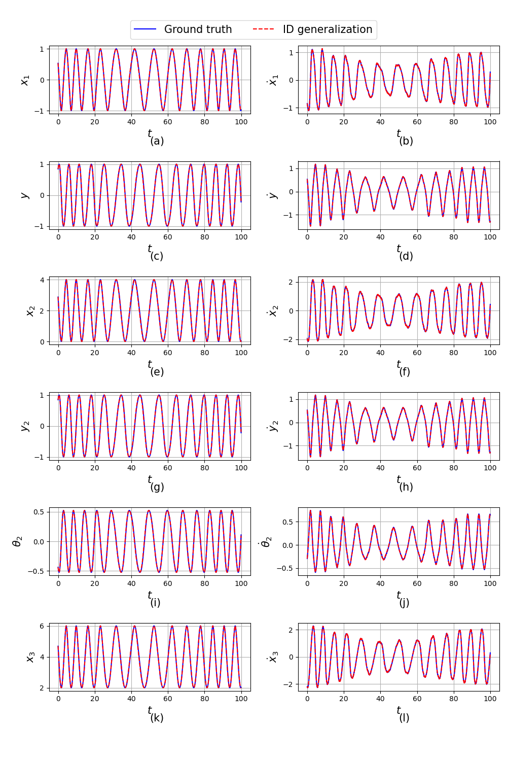
Figure 25 shows the dynamics response of the minimal coordinates under the external force and torque. MBD-NODE accurately predicts the system dynamics for the random external force and torque in the predefined range. Figure 26 shows the dynamics response of the dependent coordinates calculated from the minimal coordinates under the same external force and torque. With the combination of Fig. 26 and Fig. 25, we can see that the MBD-NODE provides good-accuracy, long-time prediction for all states. We don’t show the coordinates because they are zeros for all time.
4 Conclusion
Drawing on the NODE methodology, this work introduces MBD-NODE, a method for the data-driven modeling of MBD problems. The performance of MBD-NODE is compared against that of several state-of-the-art data-driven modeling methods by means of seven numerical examples that display attributes encountered in common real-life systems, e.g. energy conservation (single mass-spring system), energy dissipation (single mass-spring-damper system), multiscale dynamics (triple mass-spring-damper system), generalization to different parameters (single pendulum system), MPC-based control problem (cart-pole system), chaotic behavior (double pendulum system), and presence of constraints with long time prediction (slider-crank mechanism). The results demonstrate an overall superior performance of the proposed MBD-NODE method, in the following aspects:
-
1.
Generalization Capability: MBD-NODE demonstrates superior accuracy in both in-distribution (ID) and out-of-distribution (OOD) scenarios, a significant advantage over the ID-focused generalization typically observed with FCNN and LSTM models.
-
2.
Model-Based Control Application: The structure of MBD-NODE, mapping system states and external inputs to accelerations, combined with its high generalization accuracy, makes it suitable for model-based control challenges, as demonstrated in the cart-pole control problem.
-
3.
Efficiency in Data Usage and Time Independence: Unlike FCNN, MBD-NODE’s integration-based learning does not require extensive time-dependent data, enabling accurate long-term dynamics predictions with less data, as demonstrated in the slider-crank problem.
-
4.
Independence from Second-Order Derivative Data: MBD-NODE can predict second-order derivatives based on position and velocity data alone, avoiding the need for direct second-order derivative data required by FCNN and LSTM.
For reproducibility studies, we provided the open-source code base of MBD-NODE, which includes all the numerical examples and all the trained models used in this study MNODE_supportData2024 . To the best of our knowledge, this represents the first time mechanical system models and Machine Learning models are made publicly and unrestrictedly available for reproducibility studies and further research purposes. This can serve as a benchmark testbed for the future development of data-driven modeling methods for multibody dynamics problems.
5 Limitations and Future Work
The model proposed has several limitations that remain to be addressed in the future. Firstly, while the extrapolation capabilities of MBD-NODE have been tested on several problems in this work and have shown superior performance compared to traditional models like LSTM and FCNN, additional testing will paint a better picture in relation to the out-of-distribution performance of MBD-NODE. Secondly, although MBD-NODE is efficient in terms of data usage and does not rely on second-order derivative data, as detailed in this contribution, other competing methods come with less computational costs. A study to gauge the MBD-NODE trade-off between computational cost and quality of results would be justified and insightful.
Future work should also focus on optimizing the training process to reduce the MBD-NODE computational costs. Another area for improvement is extending MBD-NODE to work with flexible multibody system dynamics problems. Exploring these directions stands to enhance the practical applicability of MBD-NODE and contribute to its broader adoption.
Acknowledgements.
This work was carried out in part with support from National Science Foundation project CMMI2153855.Conflict of interest
The authors declare that they have no known competing financial interests or personal relationships that could have appeared to influence the work reported in this paper.
References
- [1] Hee Sun Choi, Junmo An, Seongji Han, Jin Gyun Kim, Jae Yoon Jung, Juhwan Choi, Grzegorz Orzechowski, Aki Mikkola, and Jin Hwan Choi. Data-driven simulation for general-purpose multibody dynamics using deep neural networks. Multibody System Dynamics, 51(4):419–454, April 2021.
- [2] Yongjun Pan, Xiaobo Nie, Zhixiong Li, and Shuitao Gu. Data-driven vehicle modeling of longitudinal dynamics based on a multibody model and deep neural networks. Measurement, 180:109541, 2021.
- [3] Myeong Seok Go, Seongji Han, Jae Hyuk Lim, and Jin Gyun Kim. An efficient fixed-time increment-based data-driven simulation for general multibody dynamics using deep neural networks. Engineering with Computers, 2023.
- [4] Seongji Han, Hee-Sun Choi, Juhwan Choi, Jin Hwan Choi, and Jin-Gyun Kim. A dnn-based data-driven modeling employing coarse sample data for real-time flexible multibody dynamics simulations. Computer Methods in Applied Mechanics and Engineering, 373:113480, 2021.
- [5] Anastasia Borovykh, Cornelis W. Oosterlee, and Sander M. Bohté. Generalization in fully-connected neural networks for time series forecasting. Journal of Computational Science, 36:101020, 2019.
- [6] Sepp Hochreiter and Jürgen Schmidhuber. Long short-term memory. Neural Comput., 9(8):1735–1780, nov 1997.
- [7] Josef Koutsoupakis and Dimitrios Giagopoulos. Drivetrain response prediction using ai-based surrogate and multibody dynamics model. Machines, 11(5), 2023.
- [8] Sönke Kraft, Julien Causse, and Aurélie Martinez. Black-box modelling of nonlinear railway vehicle dynamics for track geometry assessment using neural networks. Vehicle System Dynamics, International Journal of Vehicle Mechanics and Mobility, 57(9):1241–1270, September 2019.
- [9] Yunguang Ye, Ping Huang, Yu Sun, and Dachuan Shi. Mbsnet: A deep learning model for multibody dynamics simulation and its application to a vehicle-track system. Mechanical Systems and Signal Processing, 157:107716, 2021.
- [10] Arash Hashemi, Grzegorz Orzechowski, Aki Mikkola, and John McPhee. Multibody dynamics and control using machine learning. Multibody System Dynamics, pages 1–35, 2023.
- [11] Ricky TQ Chen, Yulia Rubanova, Jesse Bettencourt, and David K Duvenaud. Neural ordinary differential equations. Advances in neural information processing systems, 31, 2018.
- [12] Opeoluwa Owoyele and Pinaki Pal. Chemnode: A neural ordinary differential equations framework for efficient chemical kinetic solvers. Energy and AI, 7:100118, 2022.
- [13] Farshud Sorourifar, You Peng, Ivan Castillo, Linh Bui, Juan Venegas, and Joel A Paulson. Physics-enhanced neural ordinary differential equations: Application to industrial chemical reaction systems. Industrial & Engineering Chemistry Research, 62(38):15563–15577, 2023.
- [14] Gavin D Portwood, Peetak P Mitra, Mateus Dias Ribeiro, Tan Minh Nguyen, Balasubramanya T Nadiga, Juan A Saenz, Michael Chertkov, Animesh Garg, Anima Anandkumar, Andreas Dengel, et al. Turbulence forecasting via neural ode. arXiv preprint arXiv:1911.05180, 2019.
- [15] Xing Chen, Flavio Abreu Araujo, Mathieu Riou, Jacob Torrejon, Dafiné Ravelosona, Wang Kang, Weisheng Zhao, Julie Grollier, and Damien Querlioz. Forecasting the outcome of spintronic experiments with neural ordinary differential equations. Nature communications, 13(1):1016, 2022.
- [16] Alessio Quaglino, Marco Gallieri, Jonathan Masci, and Jan Koutník. Snode: Spectral discretization of neural odes for system identification. In International Conference on Learning Representations, 2019.
- [17] Chris Finlay, Joern-Henrik Jacobsen, Levon Nurbekyan, and Adam Oberman. How to train your neural ODE: the world of Jacobian and kinetic regularization. In Hal Daumé III and Aarti Singh, editors, Proceedings of the 37th International Conference on Machine Learning, volume 119 of Proceedings of Machine Learning Research, pages 3154–3164. PMLR, 13–18 Jul 2020.
- [18] Sophie Grunbacher, Ramin Hasani, Mathias Lechner, Jacek Cyranka, Scott A Smolka, and Radu Grosu. On the verification of neural odes with stochastic guarantees. In Proceedings of the AAAI Conference on Artificial Intelligence, volume 35, pages 11525–11535, 2021.
- [19] Suresh Bishnoi, Ravinder Bhattoo, Sayan Ranu, and NM Krishnan. Enhancing the inductive biases of graph neural ode for modeling dynamical systems. arXiv preprint arXiv:2209.10740, 2022.
- [20] Han Zhang, Xi Gao, Jacob Unterman, and Tom Arodz. Approximation capabilities of neural ODEs and invertible residual networks. In Hal Daumé III and Aarti Singh, editors, Proceedings of the 37th International Conference on Machine Learning, volume 119 of Proceedings of Machine Learning Research, pages 11086–11095. PMLR, 13–18 Jul 2020.
- [21] Nate Gruver, Marc Finzi, Samuel Stanton, and Andrew Gordon Wilson. Deconstructing the inductive biases of Hamiltonian neural networks. arXiv preprint arXiv:2202.04836, 2022.
- [22] Samuel Greydanus, Misko Dzamba, and Jason Yosinski. Hamiltonian neural networks. Advances in neural information processing systems, 32, 2019.
- [23] Yaofeng Desmond Zhong, Biswadip Dey, and Amit Chakraborty. Dissipative symODEN: Encoding Hamiltonian dynamics with dissipation and control into deep learning. In ICLR 2020 Workshop on Integration of Deep Neural Models and Differential Equations, 2019.
- [24] Andrew Sosanya and Sam Greydanus. Dissipative Hamiltonian neural networks: Learning dissipative and conservative dynamics separately. ArXiv, abs/2201.10085, 2022.
- [25] Peter Toth, Danilo J Rezende, Andrew Jaegle, Sébastien Racanière, Aleksandar Botev, and Irina Higgins. Hamiltonian generative networks. In International Conference on Learning Representations, 2019.
- [26] Alvaro Sanchez-Gonzalez, Victor Bapst, Kyle Cranmer, and Peter Battaglia. Hamiltonian graph networks with ode integrators. arXiv preprint arXiv:1909.12790, 2019.
- [27] Marco David and Florian Méhats. Symplectic learning for Hamiltonian neural networks. Journal of Computational Physics, 494:112495, 2023.
- [28] Zhengdao Chen, Jianyu Zhang, Martin Arjovsky, and Léon Bottou. Symplectic recurrent neural networks, 2020.
- [29] Håkon Noren, Sølve Eidnes, and Elena Celledoni. Learning dynamical systems from noisy data with inverse-explicit integrators, 2023.
- [30] Daniel M. DiPietro, Shiying Xiong, and Bo Zhu. Sparse symplectically integrated neural networks. In Advances in Neural Information Processing Systems 34. 2020.
- [31] Kiran Bacsa, Zhilu Lai, Wei Liu, Michael Todd, and Eleni Chatzi. Symplectic encoders for physics-constrained variational dynamics inference. Scientific Reports, 13(1):2643, 2023.
- [32] Miles D. Cranmer, Sam Greydanus, Stephan Hoyer, Peter W. Battaglia, David N. Spergel, and Shirley Ho. Lagrangian neural networks. CoRR, abs/2003.04630, 2020.
- [33] M Lutter, C Ritter, and Jan Peters. Deep Lagrangian networks: Using physics as model prior for deep learning. In International Conference on Learning Representations (ICLR 2019). OpenReview. net, 2019.
- [34] Marc Finzi, Ke Alexander Wang, and Andrew G Wilson. Simplifying Hamiltonian and Lagrangian neural networks via explicit constraints. Advances in neural information processing systems, 33:13880–13889, 2020.
- [35] Ravinder Bhattoo, Sayan Ranu, and NM Anoop Krishnan. Learning the dynamics of particle-based systems with Lagrangian graph neural networks. Machine Learning: Science and Technology, 4(1):015003, 2023.
- [36] Yaofeng Desmond Zhong, Biswadip Dey, and Amit Chakraborty. Extending Lagrangian and Hamiltonian neural networks with differentiable contact models. In M. Ranzato, A. Beygelzimer, Y. Dauphin, P.S. Liang, and J. Wortman Vaughan, editors, Advances in Neural Information Processing Systems, volume 34, pages 21910–21922. Curran Associates, Inc., 2021.
- [37] Jayesh K. Gupta, Kunal Menda, Zachary Manchester, and Mykel J. Kochenderfer. A general framework for structured learning of mechanical systems. CoRR, abs/1902.08705, 2019.
- [38] Ahmed A Shabana. Dynamics of multibody systems. Cambridge university press, 2020.
- [39] Olivier A. Bauchau and André Laulusa. Review of Contemporary Approaches for Constraint Enforcement in Multibody Systems. Journal of Computational and Nonlinear Dynamics, 3(1):011005, 11 2007.
- [40] Juntang Zhuang, Nicha Dvornek, Xiaoxiao Li, Sekhar Tatikonda, Xenophon Papademetris, and James Duncan. Adaptive checkpoint adjoint method for gradient estimation in neural ODE. In Hal Daumé III and Aarti Singh, editors, Proceedings of the 37th International Conference on Machine Learning, volume 119 of Proceedings of Machine Learning Research, pages 11639–11649. PMLR, 13–18 Jul 2020.
- [41] Kookjin Lee and Eric J Parish. Parameterized neural ordinary differential equations: Applications to computational physics problems. Proceedings of the Royal Society A, 477(2253):20210162, 2021.
- [42] Alexander Norcliffe, Cristian Bodnar, Ben Day, Nikola Simidjievski, and Pietro Lió. On second order behaviour in augmented neural odes. In H. Larochelle, M. Ranzato, R. Hadsell, M.F. Balcan, and H. Lin, editors, Advances in Neural Information Processing Systems, volume 33, pages 5911–5921. Curran Associates, Inc., 2020.
- [43] Guan-Horng Liu, Tianrong Chen, and Evangelos Theodorou. Second-order neural ode optimizer. Advances in Neural Information Processing Systems, 34:25267–25279, 2021.
- [44] Chigozie Nwankpa, Winifred L. Ijomah, Anthony Gachagan, and Stephen Marshall. Activation functions: Comparison of trends in practice and research for deep learning. ArXiv, abs/1811.03378, 2018.
- [45] Xavier Glorot and Yoshua Bengio. Understanding the difficulty of training deep feedforward neural networks. In Yee Whye Teh and Mike Titterington, editors, Proceedings of the Thirteenth International Conference on Artificial Intelligence and Statistics, volume 9 of Proceedings of Machine Learning Research, pages 249–256, Chia Laguna Resort, Sardinia, Italy, 13–15 May 2010. PMLR.
- [46] Kaiming He, Xiangyu Zhang, Shaoqing Ren, and Jian Sun. Delving deep into rectifiers: Surpassing human-level performance on imagenet classification. In Proceedings of the IEEE international conference on computer vision, pages 1026–1034, 2015.
- [47] Takashi Matsubara, Yuto Miyatake, and Takaharu Yaguchi. Symplectic adjoint method for exact gradient of neural ode with minimal memory. In M. Ranzato, A. Beygelzimer, Y. Dauphin, P.S. Liang, and J. Wortman Vaughan, editors, Advances in Neural Information Processing Systems, volume 34, pages 20772–20784. Curran Associates, Inc., 2021.
- [48] Michel Fortin and Roland Glowinski. Augmented Lagrangian methods: applications to the numerical solution of boundary-value problems. Elsevier, 2000.
- [49] Lu Lu, Raphaël Pestourie, Wenjie Yao, Zhicheng Wang, Francesc Verdugo, and Steven G. Johnson. Physics-informed neural networks with hard constraints for inverse design. SIAM Journal on Scientific Computing, 43(6):B1105–B1132, 2021.
- [50] Yi Heng Lim and Muhammad Firmansyah Kasim. Unifying physical systems’ inductive biases in neural ode using dynamics constraints. In ICML 2022 2nd AI for Science Workshop, 2022.
- [51] Franck Djeumou, Cyrus Neary, Eric Goubault, Sylvie Putot, and Ufuk Topcu. Neural networks with physics-informed architectures and constraints for dynamical systems modeling. In Roya Firoozi, Negar Mehr, Esen Yel, Rika Antonova, Jeannette Bohg, Mac Schwager, and Mykel Kochenderfer, editors, Proceedings of The 4th Annual Learning for Dynamics and Control Conference, volume 168 of Proceedings of Machine Learning Research, pages 263–277. PMLR, 23–24 Jun 2022.
- [52] R. A. Wehage and E. J. Haug. Generalized coordinate partitioning for dimension reduction in analysis of constrained dynamic systems. J. Mech. Design, 104:247–255, 1982.
- [53] Tom Beucler, Michael Pritchard, Stephan Rasp, Jordan Ott, Pierre Baldi, and Pierre Gentine. Enforcing analytic constraints in neural networks emulating physical systems. Physical Review Letters, 126(9):098302, 2021.
- [54] Rembert Daems, Jeroen Taets, Guillaume Crevecoeur, et al. Keycld: Learning constrained Lagrangian dynamics in keypoint coordinates from images. arXiv preprint arXiv:2206.11030, 2022.
- [55] Jingquan Wang, Shu Wang, Huzaifa Unjhawala, Jinlong Wu, and Dan Negrut. Models, scripts, and meta-data: Physics-informed data-driven modeling and simulation of constrained multibody systems. https://github.com/uwsbel/sbel-reproducibility/tree/master/2024/MNODE-code, 2024.
- [56] Yuhan Chen, Takashi Matsubara, and Takaharu Yaguchi. Neural symplectic form: Learning Hamiltonian equations on general coordinate systems. In A. Beygelzimer, Y. Dauphin, P. Liang, and J. Wortman Vaughan, editors, Advances in Neural Information Processing Systems, 2021.
- [57] Sophie Steger, Franz Martin Rohrhofer, and Bernhard Geiger. How pinns cheat: Predicting chaotic motion of a double pendulum. 2022. The Symbiosis of Deep Learning and Differential Equations II @ the 36th Neural Information Processing Systems (NeurIPS) Conference ; Conference date: 09-12-2022.
- [58] Basil Kouvaritakis and Mark Cannon. Model predictive control. Switzerland: Springer International Publishing, 38:13–56, 2016.
Appendix A Algorithms for training the MNODE
Appendix B Training time cost for different models and integrators
| Test Case | Model | Integrator | Time Cost (s) |
|---|---|---|---|
| Single Mass Spring | MNODE | LF2 | 507.73 |
| MNODE | YS4 | 874.05 | |
| MNODE | FK6 | 1461.52 | |
| HNN | RK4 | 218.02 | |
| LNN | RK4 | 988.45 | |
| Single Mass Spring Damper | MNODE | FE1 | 316.86 |
| MNODE | MP2 | 518.09 | |
| MNODE | RK4 | 1254.13 | |
| FCNN | - | 220.13 | |
| LSTM | - | 500.63 | |
| Triple Mass Spring Damper | MNODE | FE1 | 358.55 |
| MNODE | MP2 | 608.55 | |
| MNODE | RK4 | 915.68 | |
| FCNN | - | 214.13 | |
| LSTM | - | 460.33 | |
| Single Pendulum | MNODE | FE1 | 250.52 |
| MNODE | MP2 | 276.12 | |
| MNODE | RK4 | 838.37 | |
| FCNN | - | 210.18 | |
| LSTM | - | 348.36 | |
| Double Pendulum | MNODE | FE1 | 253.34 |
| MNODE | MP2 | 368.75 | |
| MNODE | RK4 | 854.06 | |
| FCNN | - | 176.51 | |
| LSTM | - | 402.62 | |
| Cart-pole | MNODE | FE1 | 255.80 |
| MNODE | MP2 | 285.04 | |
| MNODE | RK4 | 776.08 | |
| FCNN | - | 214.26 | |
| LSTM | - | 358.14 |
Appendix C The detail formulation of the equation of motion for the slider-crank mechanism
Following the setting mentioned in Section 3.7, the equation of motion for the slider-crank mechanism can be formulated as follows:
The mass matrix is:
| (50) |
where:
The states of the slider crank mechanism follows the below constraints on the position:
| (51) |
We also have the following constraints on the velocit:
| (52) |
The vector from external forces is:
| (53) |
where:
We can rearrange the constraint equations on the acceleration:
| (54a) | ||||
| (54b) | ||||
| (54c) | ||||
| (54d) | ||||
| (54e) | ||||
| (54f) | ||||
| (54g) | ||||
| (54h) | ||||
to get the as:
| (55) |
Finally, we plug the above equations into Eq. 1 to get the equation of motion for the slider-crank mechanism.