Many wrong models approach to localize an odor source in turbulence:
introducing the weighted Bayesian update

Abstract

The problem of locating an odor source in turbulent environments is central to key applications such as environmental monitoring and disaster response. We address this challenge by designing an algorithm based on Bayesian inference, which uses odor measurements from an ensemble of static sensors to estimate the source position through a stochastic model of the environment. Given the practical impossibility of achieving a fully consistent turbulent model and guaranteeing convergence to the correct solution, we propose a method to rank “many wrong models” and to blend their predictions. We evaluate our weighted Bayesian update algorithm by its ability to estimate the source location with predefined accuracy and/or within a specified time frame, and compare it to standard Monte Carlo sampling methods. To demonstrate the robustness and potential applications of both approaches under realistic environmental conditions, we use high-quality direct numerical simulations of the Navier-Stokes equations to mimic the transport of odors in the atmospheric boundary layer. Despite minimal prior information about the source and environmental conditions, our proposed approach consistently proves to be more accurate, reliable, and robust than Monte Carlo methods, thus showing promise as a new tool for addressing the odor source localization problem in real-world scenarios.

I Introduction

Identifying the origin of noxious odors such as gas leaks and chemical or radioactive emissions is critical for averting potential environmental disasters [1, 2, 3, 4]. Moreover, tracing the location of a source from the odor signal detected in the atmosphere is a vital task for animals looking for food or a mate [5, 6].

Such source localization problems are already difficult in laminar flows, where the structure of the odor plume can be highly complex and sensitive to the source location due to chaotic mixing [7, 8]. In fully turbulent three-dimensional (3-D) environments, the difficulty becomes severe, owing to numerical, experimental, and phenomenological complexities and challenges associated with the multi-scale nature of 3-D turbulence, which is characterized by a broad range of rough velocity fluctuations as well as highly intermittent and non-Gaussian properties for both the advecting flow and the odor transport [9, 10, 11, 12].

This makes the design of efficient and reliable algorithms for source localization a challenging theoretical task situated at the intersection of fluid dynamics, optimal navigation of mobile agents, and information theory [12, 13, 14]. Over the last decades, a growing community of scientists has developed multiple methodologies to address this problem, ranging from bio-inspired [15, 16, 17] to heuristic search algorithms based on information theory [18, 19, 20] and Bayesian inference [21, 22].

Although most studies have focused on the performance optimization of mobile agents, the use of static sensors has become increasingly popular [23, 24, 25] thanks to the simplicity of their implementation, also resulting in reduced setup and maintenance costs. Moreover, being well-suited for continuous and large-scale environmental monitoring, they are ideal for use in early warning systems [26, 27, 28, 29], which may enable targeted and effective response strategies, ranging from containment and mitigation to rescue and prevention. On a more theoretical level, the employment of static sensors reduces the space of possible choices for the search algorithm [30], thereby facilitating the study of more fundamental questions. Indeed, despite the recent progress, the problem of optimally locating a source within a given time with a prescribed accuracy in a turbulent flow is far from solved [25].

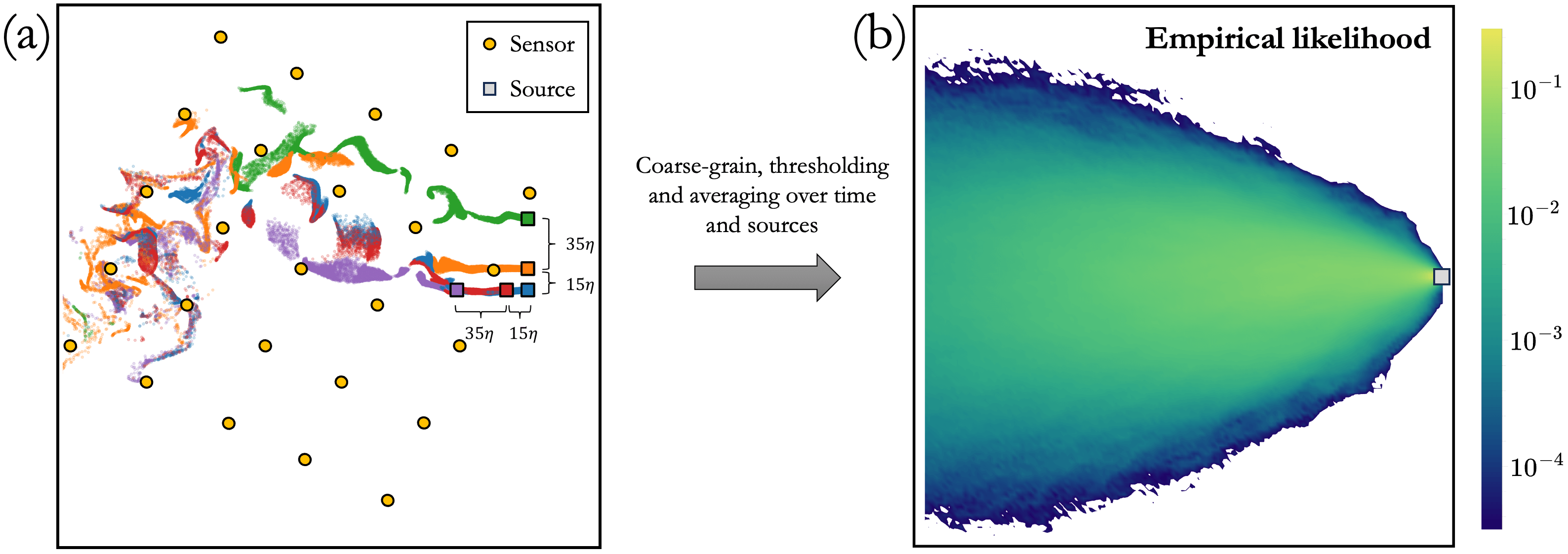
Figure 1: Left: a snapshot of DNS showing relative positions of sources (squares) and particles color-coded according to the source from which each was emitted. Here, we show particles in a thin slab parallel to the wind and containing the sources, and we have zoomed in close to the sources. We have also inserted in the same plane a network of static sensors (yellow circles) whose measurements will be used in the following to infer the source location. Right: probability map of making a detection. Hereafter referred to as empirical likelihood, such distribution has been obtained from coarse-graining the DNS data on a square lattice, setting a threshold $n_{\rm thr}=2$ on the number of detectable particles, and then averaging over time the signal of all the five sources (properly placed, by means of a suitable shift, in the same position as indicated by the grey square).

A key challenge is the practical impossibility of specifying a detailed model for the statistics governing odor transport. This is a crucial point when using Bayesian approaches that heavily depend on a model of the environment to integrate sensor observations into a probability distribution describing our information about the source. However, in all real-world applications, we have only partial knowledge of the statistical properties of the environment, which may be arbitrarily complex. Moreover, the inherent complexity of turbulent transport precludes a complete analytical description even in an idealized physical scenario. Therefore, we are invariably compelled to work with an wrong model of the environment. This fundamentally limits the utility of Bayesian approaches, which are only guaranteed to converge to the ground truth when the model is correctly specified [31, 32]. To partially overcome these intrinsic limitations, we explore a new Bayesian approach designed to mitigate the effects of errors in the environmental model. Building upon the many wrongs principle [33, 34], we introduce a quantity that allows to rank the models of the environment in the Bayesian framework, providing a principled way to blend information coming from several (inevitably wrong) models. We show that merging the information gathered from a number of different models – a procedure that we dubbed Weighted Bayesian Update (WBU) – helps in reliably inferring the source location.

In order to test these ideas and the proposed methodology in realistic conditions, we devise a set of direct numerical simulations that mimic the emission of a localized odor source in a three-dimensional turbulent environment. Taking advantage of the Galilean invariance of the Navier-Stokes equation, we model the odor transport by Lagrangian tracers advected by the flow with a constant mean wind, obtaining odor plumes that well approximate those one can observe in the atmospheric boundary layer [11, 12]. Here, for the sake of a first benchmark of the localization algorithms, we shall assume the source lies on the same plane as the sensors, which can thus detect odor particles contained in a thin slab parallel to the wind [see Fig.1(a)]. Then, we use a simplified (effective) model for the environment that depends on a few parameters only and neglects temporal and spatial correlations of the odor signal. In spite of the obvious shortcomings of this model, we show how, by suitably weighting different models (i.e. the same one with different parameters), WBU outperforms widely-used Monte Carlo methods [21, 35] when locating the odor source with a specified level of accuracy. By performing several tests with synthetic data and empirically based (a posteriori) models, we trace the origin of the problems for Monte Carlo methods to the effects of correlations in the realistic odor signal, to which the WBU shows superior resilience.

The paper is organized as follows. In Sec. II, we illustrate the setup where the numerical simulations have been carried out and describe the simplified model of the environment as well as the algorithms employed, namely the weighted Bayesian update and another approach based on Monte Carlo techniques. We then present the results in Sec. III, which is divided into two parts. In the first one, Sec. III.1, we discuss and compare the performance of the algorithms in the setting closest to reality. In Sec. III.2, we then systematically study how model inaccuracy affects the quality of the source localization. Finally, we summarize our findings and provide an outlook for future studies in Sec. IV.

II Methods

II.1 Setup of the numerical simulations

Let us assume we aim to locate the position $\bm{r}_{\rm s}$ of an odor source emitting at rate $Q$ within a two-dimensional square grid $\Omega$ of size $L\times L$ and lattice spacing $\Delta x$. The odor particles are swept by the underlying turbulent flow characterized by a mean wind in a given direction $\hat{\bm{U}}$. We then place a number $N_{\rm s}$ of static sensors in this environment. We arrange the sensors in a lattice that, assuming no prior knowledge of the wind direction, will be typically tilted by an angle $\theta$ with respect to the latter, as depicted in Fig. 1(a).

Instead of using an odor concentration field, we model it in terms of particles advected by a turbulent flow. Each particle can be thought of as a patch of odor, or one can consider the number of particles in a given small region as an estimate of the odor concentration. We produced realistic trajectories of odor particles using state-of-the-art direct numerical simulation (DNS) of the incompressible, 3–D Navier-Stokes equations

$$\partial_{t}\bm{u}+(\bm{u}\cdot\nabla)\bm{u} =-\nabla p+\nu\nabla^{2}\bm{u}+f,$$ (1)

$$\nabla\cdot\bm{u} =0,$$ (2)

under turbulent conditions with $\mathrm{Re}_{\lambda}\simeq 150.$ Here, $f$ is a random, Sawford-type [36] isotropic forcing at the smallest nonzero wavenumbers of the system, with a correlation time of 160 simulation timesteps. Using a pseudospectral code dealiased according to the two-thirds rule, the system was solved on a $1024\times 512\times 512$ grid, with a uniform spacing $\delta x=\delta y=\delta z\simeq\eta$ (with $\eta$ the Kolmogorov scale), and periodic boundary conditions in all three directions. The timestepping was performed using the second-order explicit Adams-Bashforth method. The system was advected by a uniform mean wind $\bm{U}\approx-2.5u_{\rm rms}\hat{x},$ where $u_{\rm rms}$ is the rms speed of the flow in the comoving frame of the wind, and $\hat{x}$ is the elongated axis of the grid. We produced the mean wind by means of a Galilean transformation.

The odor particles were modeled as Lagrangian tracer particles, which were emitted by five stationary point sources [Fig. 1(a)]. Each source emitted 1000 particles every 10 simulation timesteps, which corresponds to every $\approx 1/15$ Kolmogorov times $\tau_{\eta}$. The fluid velocities $\bm{u}$ at the particle positions were obtained using a sixth-order B-spline interpolation scheme and then used to evolve the particle positions $\bm{X}$ in time according to $\dot{\bm{X}}=\bm{u}(\bm{X},t)$ over an infinite lattice of copies of the periodic flow. Their positions, velocities, and accelerations were tracked and dumped every $\tau_{\eta},$ for a total of 3015 timesteps. Each source of particles was treated as independent, and we averaged our results over them for the purpose of achieving better statistics.

To simulate realistic environmental conditions and emulate turbulent dispersion in the atmospheric boundary layer, we then coarse-grain the particles’ concentration inside a thin layer containing the source and set a threshold $n_{\rm thr}=2$ on the number of particles above which sensors make a detection. A few snapshots of the resulting odor dispersion in the aforementioned arena $\Omega$ are shown in Fig. 2, where the pink patches indicate the odor plume.

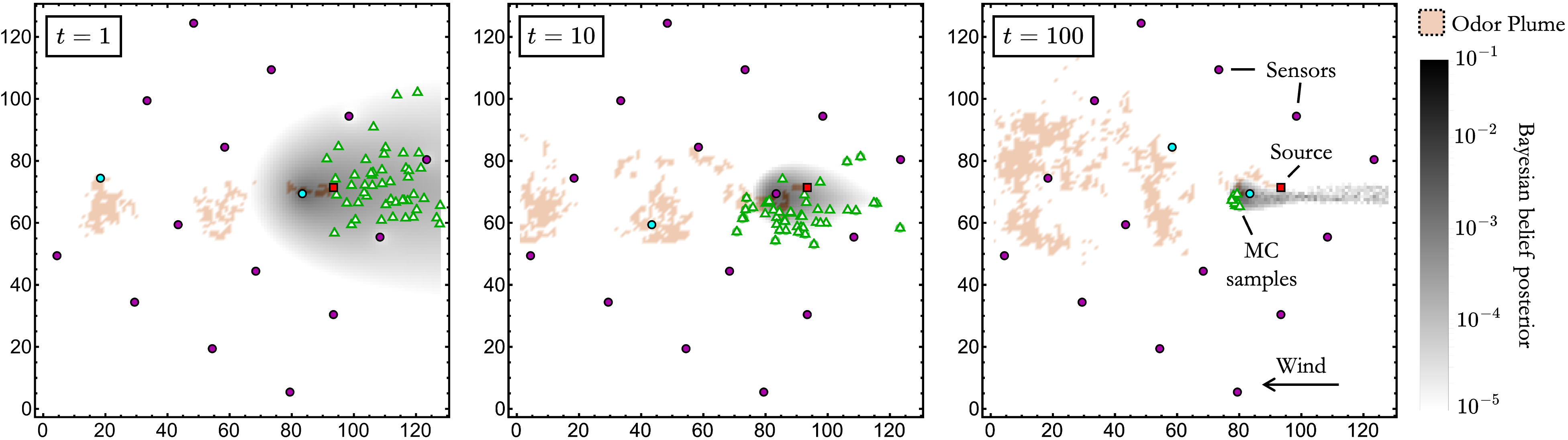
Figure 2: Three time snapshots showing a qualitative comparison between the performance of the two algorithms discussed in this work. Both approaches use the measurements made by an array of static sensors (circles) looking for a source of odors (red square) advected by a turbulent flow featuring a horizontal wind blowing from right to left. Pink patches indicate the odor plume; greyscale codes the probability of the odor source location obtained from an algorithm based on Bayesian inference; green open triangles depict the candidate source positions yielded by a Sequential Monte Carlo sampling method. Time here is in units of observations made by each sensor, which is hereafter assumed to be equal to the Kolmogorov timescale $\tau_{\eta}$ of the flow.

II.2 Model of the environment

To localize the source within this setting given the sensors’ measurements, we shall now introduce a model that captures the mean-flow and mean-diffusion properties of the environment. If, on the one hand, we assume to have a statistical knowledge of the environment through, for example, the history of prior measurements in the field, we can compute empirically what is the probability of detecting an odor particle from the time average of the DNS data [Fig. 1(b)]. We will hereafter refer to this distribution as the empirical likelihood, in accordance with Bayesian nomenclature. The use of such likelihood has the advantage of avoiding the complication of fitting some environmental parameters while looking for the source. However, it relies on a far more detailed prior knowledge of the environment, which is not generally available. On the other hand, we can still exploit it to understand the strengths and weaknesses of the localization algorithms, as discussed in Sec. III.2.

In a realistic setup, we are therefore compelled to use a statistical description of odor encounters in a turbulent flow to infer the source location. Out of a wide range of possibilities [37], we model the turbulent transport of odor particles emitted at rate $Q$ by a point source as an effective advection-diffusion process [38]

$$\partial_{t}c+\bm{U}\cdot\bm{\nabla}c=D\nabla^{2}c+Q\delta(\bm{r}-\bm{r}_{\rm s})-c/\tau\,,$$ (3)

where $c$ is the odor concentration field, $\bm{U}$ the mean wind featured by the turbulent flow, $\tau$ the lifetime of the odors, and $\bm{r}_{\rm s}$ the source position. Note that the combination of molecular and turbulent diffusivity (due to the flow velocity fluctuations) is here described by a single effective (eddy) diffusion coefficient $D$ [39]. Despite being a strong oversimplification that ignores important multiscale, non-Gaussian properties of the underlying turbulence, as well as spatiotemporal fluctuations in the scalar advection, this model reasonably captures the mean field properties of the odor concentration [12]. In the stationary regime, Eq. (3) has an analytical solution, which in three dimensions reads (see, e.g., [18])

$$c(\bm{r}-\bm{r}_{\rm s})=\frac{Q}{4\pi D\lVert\bm{r}-\bm{r}_{\rm s}\rVert}\exp\left[\frac{(\bm{r}-\bm{r}_{\rm s})\cdot\hat{\bm{U}}-\lVert\bm{r}-\bm{r}_{\rm s}\rVert}{\lambda}\right]\,,$$ (4)

where we have assumed $\tau\gg 1$. A key advantage of the adopted model is that it essentially depends only on three environmental parameters, i.e., the source emission rate $Q$, the mean wind direction $\hat{\bm{U}}$, and the characteristic length scale of the flow $\lambda\equiv 2D/U$. To mimic the sparseness and intermittency of the odor signals observed from the DNS, and typical of turbulent environments, we assume that the detection is a random process modeled in terms of a Poissonian process with mean $\mu$ [18, 40]. Therefore, the probability that a sensor makes a detection is given by

$$p(h_{i}|\bm{r}_{i}-\bm{r}_{\rm s})=\frac{[\mu(\bm{r}_{i}-\bm{r}_{\rm s})]^{h_{i}}\exp[-\mu(\bm{r}_{i}-\bm{r}_{\rm s})]}{h_{i}!}\,,$$ (5)

where $h_{i}$ is the number of odor particles detected by the $i-$th sensor. The mean number $\mu$ of particles hitting, within a time interval $\Delta t$, the $i$-th sensor is related to the mean concentration (4) via the classical Smoluchowski formula [41]

$$\mu(\bm{r}_{i}-\bm{r}_{\rm s})=4\pi aD\Delta t\,c(\bm{r}_{i}-\bm{r}_{\rm s})=\frac{Q}{d_{i}}a\Delta t\exp\left[\frac{(\bm{r}_{i}-\bm{r}_{\rm s})\cdot\hat{\bm{U}}-d_{i}}{\lambda}\right]\,,$$ (6)

where $\bm{r}_{i}$ stands for the $i-$th sensor position, and $d_{i}\equiv\lVert\bm{r}_{i}-\bm{r}_{\rm s}\rVert$, $a$ is the sensors’ radius. Hereafter, we will actually assume that each sensor can detect the presence of odors only if the number of particles within its radius $a=\Delta x/2$ exceeds a particular threshold. In other words, the sensors can only perform binary measurements (i.e., $h_{i}=\{0,1\}$), such that the probability of detection (5) simplifies into

$$\begin{cases}p(0|\bm{r}_{i}-\bm{r}_{\rm s})=\exp[-\mu(\bm{r}_{i}-\bm{r}_{\rm s})]\\ p(1|\bm{r}_{i}-\bm{r}_{\rm s})=1-\exp[-\mu(\bm{r}_{i}-\bm{r}_{\rm s})]\,.\end{cases}$$ (7)

II.3 Weighted Bayesian Update: a new way to rank and exploit many wrong models

Each measurement made by each sensor thus provides information about the position of the source $\bm{r}_{\rm s}$, which can be processed employing Bayesian inference. The whole set of measurements from all sensors can be used to update a probability map – the “posterior” or “belief” in Bayesian jargon – of the source’s location defined over the whole arena $\Omega$, i.e. $B(\bm{r})\equiv\mathrm{Prob}(\bm{r}_{\rm s}=\bm{r})$, which we shall dub as common belief to emphasize that it exploits all sensors’ detections. Since we assume no prior knowledge and that the source cannot be at the same location as one of the sensors, the belief is always initialized to a uniform distribution and set to zero only in the sensors’ positions. Assuming the simultaneous measurements made by all the $N_{\rm s}$ sensors at time $t$ are independent, the overall conditional probability of a set of observations $\bm{h}^{(t)}$ for a possible given source position $\bm{r}$ is simply a product:

$$\mathcal{L}(\bm{h}^{(t)}|\bm{r})=\prod\limits_{i=1}^{N_{\rm s}}p(h_{i}^{(t)}|\bm{r}_{i}-\bm{r})\,,$$ (8)

which depends on the model of the environment as specified in Eq. (7), and is also known as the likelihood function in Bayesian terminology. Given a sequential process like the one at hand, at every time step (i.e., once all sensors have performed a measurement), the belief is updated following Bayes’ rule [42]

$$B^{(t)}(\bm{r})=\frac{\mathcal{L}(\bm{h}^{(t)}|\bm{r})B^{(t-1)}(\bm{r})}{\int_{\Omega}{\rm d}\bm{r}\,\mathcal{L}(\bm{h}^{(t)}|\bm{r})B^{(t-1)}(\bm{r})}\,,$$ (9)

where time $t$ is hereafter measured in units of observations made by each sensor.

Under this update rule, the belief is guaranteed to converge to the correct solution as long as the correct model of the environment is deployed [43]. This is, however, a rather uncommon case in any realistic scenario, and the model used to update the common belief will always be wrong. Furthermore, wrong models are indistinguishable from one another during the search since they always make the belief converge to a source position, regardless of whether that is the right one or not. Therefore, finding a way to rank the models and assess their reliability is of great relevance for any applications.

In order to introduce the quantity we used for ranking the models, it is useful to rewrite Bayes’ update rule (9) in a different way:

$$B^{(t)}(\bm{r})=\frac{\prod\limits_{i=1}^{N_{\rm s}}b_{i}^{(t)}(\bm{r})}{\mathcal{Z}}\,,\;\;\;\;\;\;b_{i}^{(t)}(\bm{r})=\frac{p(h_{i}^{(t)}|\bm{r}_{i}-\bm{r})b_{i}^{(t-1)}(\bm{r})}{\int_{\Omega}{\rm d}\bm{r}\,p(h_{i}^{(t)}|\bm{r}_{i}-\bm{r})b_{i}^{(t-1)}(\bm{r})}\,,$$ (10)

where $\mathcal{Z}\equiv\int_{\Omega}{\rm d}\bm{r}\,\prod\limits_{i=1}^{N_{\rm s}}b_{i}^{(t)}(\bm{r})$. That is to say, owing to the assumption of independence between measurements, the common belief can be built from the superposition of the private beliefs (i.e. the belief that can be constructed for each sensor only on the basis of its own measurements history) $b_{i}$ of the $i=1,...,N_{\rm s}$ sensors, each of which is updated independently at every time step via Bayes’ rule. The key advantage of this change of perspective lies in the interpretation of the update formula [Eqs. (9-10)]. Indeed, the hitherto overlooked normalization constant $\mathcal{Z}$ essentially quantifies how much the sensors’ private beliefs overlap or, in other words, how much they agree on a source position given their measurements and the model at hand. In fact, in Appendix A, we show analytically that this quantity achieves an asymptotic global maximum when the model is exact (even in the presence of correlations between observations). We also show numerically that this quantity is typically smaller the farther the model is from the ground truth.

This makes $\mathcal{Z}$, hereafter referred to as the overlap integral, an ideal candidate to achieve our task as we could use it to weigh different models of the environment. To this end, let us scan the parameters space of the stochastic model introduced above [see Eqs. (6)-(7)] assuming to know only on the mean wind direction $\hat{\bm{U}}$, which can be always measured in practice using an anemometer, and run the Bayes update (9) independently for each set of parameters $\bm{P}\equiv\{Q,\lambda\}$. Then, we shall blend the information collected into a master belief as

$$\mathcal{B}^{(t)}_{\rm M}(\bm{r})=\frac{\prod\limits_{j=1}^{M}\left[B_{j}^{(t)}(\bm{r})\right]^{\beta_{j}^{(t)}}}{\int_{\Omega}\prod\limits_{j=1}^{M}\left[B_{j}^{(t)}(\bm{r})\right]^{\beta_{j}^{(t)}}}\,,\;\;\;\beta_{j}^{(t)}\equiv\frac{\mathcal{Z}_{j}^{(t)}}{\sum\limits_{j=1}^{M}\mathcal{Z}_{j}^{(t)}}\,,$$ (11)

where $M$ is the total number of distinct sets $\bm{P}_{j}=\{Q_{j},\lambda_{j}\}$ of model parameters considered, and the index $j$ refers to which of these sets was used to obtain the common belief $B_{j}^{(t)}$ at time $t$ and the corresponding overlap integral $\mathcal{Z}_{j}^{(t)}$.

The algorithmic procedure described in Eqs. (9)$-$(11) thus provides a principled way to define a single master belief $\mathcal{B}_{\rm M}$, i.e.,  the probability distribution about the source location, which is obtained from a weighted average over the results yielded by different models. We will hereafter refer to this approach as the weighted Bayesian update (WBU), whose numerical implementation is detailed in Appendix B.

II.4 Sequential Monte Carlo with Importance Sampling

The above-described WBU method offers a new perspective on the implementation of algorithms for odor source localization in turbulent flows. There exists, however, already a vast literature on the possible methods to address the same kind of problem [25]. One of the most commonly used approaches is the one based on the use of Monte Carlo sampling methods to estimate the belief [21, 40, 35]. It is, therefore, natural to ask how the WBU’s performance compares with such more conventional approaches.

Due to the wide range of potential applications [44], much research has been conducted over the last decades to make these algorithms more and more computationally efficient and accurate, and, to date, there exist many different variants depending on the specific setup at hand. We refer the reader to Ref. [25] for a comprehensive review of the topic.

In the following, we shall use a state-of-the-art version of the so-called Sequential Monte Carlo (SMC) algorithm that also involves a Markov chain Monte Carlo (MCMC) perturbation step [45, 46]. Using such an approach, we can simultaneously infer both the source position $\bm{r}_{\rm s}$ and the (unknown) parameters $\bm{P}$ of the stochastic model of the environment. Let us therefore first define a sample $\bm{\theta}_{i}$ as a possible combination of such source parameters, i.e. $\bm{\theta}_{i}\equiv\{\bm{r}_{{\rm s},i},\bm{P}_{i}\}$. At every time step, after all sensors have measured, a collection of $N$ of such samples is drawn from the current belief defined in the $\bm{\theta}$ space, and we assign a weight $w$ to each of them equal to the likelihood of the latest measurement as defined in Eq. (8). Upon normalization of the samples’ weights, we shall then compute the effective sample size $N_{\rm eff}$ to avoid the so-called degeneracy problem [46]. Indeed, if $N_{\rm eff}$ goes below a given threshold $N_{\rm thr}$ (typically set to $N/2$), then it is necessary to generate a new set of $N$ samples. This is known as the resampling step. There, for each sample $\tilde{\bm{\theta}}_{i}$, a new one is selected from the same pool and with a probability equal to its weight that replaces the former. After resampling, all weights are then set equal to $1/N$.

Next is the so-called Metropolis-Hastings MCMC perturbation step, which consists of moving each sample in its neighborhood and deciding whether to accept or reject the new proposal based on some acceptance criteria [47]. This is essentially done to diversify the $N$ samples and, therefore, improve the sampling efficiency of the Monte Carlo algorithm [46]. More specifically, starting from one of the samples at time $t$, say $\tilde{\bm{\theta}}_{i}^{(t)}$, a Markov chain of length $K$ is generated where new inferences $\hat{\bm{\theta}}^{(t)}$ are drawn from the previous link in the chain, $\tilde{\bm{\theta}}_{i,j-1}^{(t)}$, using a proposal distribution $q(\hat{\bm{\theta}}^{(t)}|\tilde{\bm{\theta}}_{i,j-1}^{(t)})$. Although there exist several valid choices for this distribution [48], here we shall use a Gaussian with a mean $\mu=\tilde{\bm{\theta}}_{i,j-1}^{(t)}$ and variance $\sigma^{2}$ as a free hyperparameter, i.e. $q(\hat{\bm{\theta}}^{(t)}|\bm{\theta}^{(t)}_{i,j-1})=\mathcal{N}(\bm{\theta}^{(t)}_{i,j-1},\sigma^{2})$. Once the new sample is generated, we shall compute the so-called acceptance ratio [45]

$$\alpha=\prod\limits_{k=1}^{t}\left[\frac{\mathcal{L}(\bm{h}^{(k)}|\hat{\bm{\theta}}^{(k)})}{\mathcal{L}(\bm{h}^{(k)}|\bm{\theta}^{(k)}_{i,j-1})}\right]\frac{q(\bm{\theta}^{(t)}_{i,j-1}|\hat{\bm{\theta}}^{(t)})}{q(\hat{\bm{\theta}}^{(t)}|\bm{\theta}^{(t)}_{i,j-1})}\,,$$ (12)

which basically amounts to the likelihood’s history ratio (also known as the posterior ratio) divided by the proposal ratio. Including the latter is necessary to correct a bias in the proposal distribution if it is asymmetric [45]. The proposed sample $\hat{\bm{\theta}}^{(t)}$ will then be accepted as a new link in the chain as long as $\alpha>1$, and with probability $\alpha$ otherwise.

Finally, once all samples have been perturbed, we are left with a new approximation of the belief, which reads: $\tilde{B}^{(t)}(\bm{\theta})=1/N\sum_{i=1}^{N}\delta(\bm{\theta}-\bm{\theta}^{(t)}_{i})$. A detailed step-by-step description of the procedure outlined above is given in Appendix B.

Analogous to what we observed in the Bayesian update, once the SMC algorithm’s hyperparameters are properly adjusted, it will systematically converge to the correct source location as long as the model of the environment is functionally exact. However, it is not clear how this approach would compare with the WBU one in a realistic scenario where it uses an inevitably misspecified model of the environment.

III Results

III.1 Stop criterion for source localization

The performance of localization algorithms is typically judged based on their ability to estimate the odor source position with a specified accuracy or within a given time limit [25, 49, 50]. However, more generally, we shall test the reliability of such algorithms by envisioning their application in a real-world scenario, where we do not know a priori where the source is and have to decide when to stop looking for it. Therefore, for an algorithm to be effective in practice, it must show a correlation between an observable quantity and the quality of its estimate of the source location.

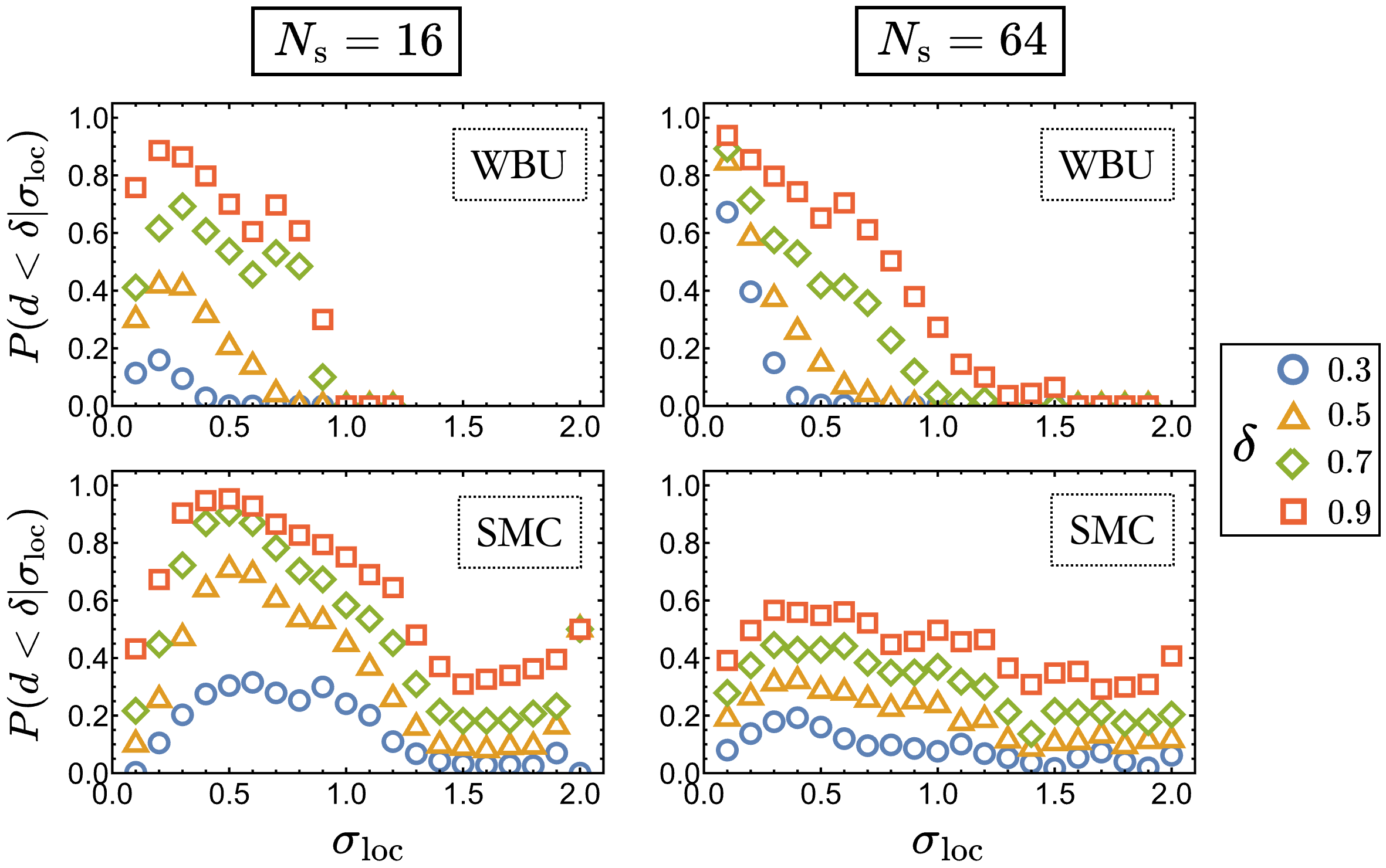
Figure 3: Four panels showing the probability that the distance $d$ between the estimated source position $\bm{\bar{r}}$ and the ground truth $\bm{r}_{\rm s}$ is below a given threshold $\delta$ (indicated in the legend) as a function of the belief/sample standard deviation $\sigma_{\rm loc}$. Lengths are in units of the distance between sensors. The columns differ in the number of sensors, while the two rows correspond to the algorithm used (top: WBU, bottom: SMC).

To this end, a good candidate quantity is the current uncertainty one has about the source location. This can be formally defined in the WBU approach as the variance of the master belief (11), which reads

$$\sigma^{2}_{\rm loc}\equiv\int_{\Omega}\,{\rm d}\bm{r}\,\mathcal{B}_{\rm M}(\bm{r})(\bm{r}-\bm{\bar{r}})^{2}\,,$$ (13)

where $\bm{\bar{r}}\equiv\int_{\Omega}\,{\rm d}\bm{r}\,\mathcal{B}_{\rm M}(\bm{r})\bm{r}$ is the estimated source location .

In the ideal case where the model of the environment is exact, $\sigma^{2}_{\rm loc}$ would be inversely correlated with how close the estimated position is to the ground truth. In other words, the smaller the variance of the belief, the more accurate the source location estimate would be. However, the exact model of the environment is inaccessible to us in any practical scenario. Therefore, such correlation is not guaranteed to hold in general and may depend on the algorithmic procedure employed.

We shall thus quantify the robustness of a given localization algorithm by looking at the probability $P(d<\delta|\sigma_{\rm loc})$ that the distance $d$ between $\bm{\bar{r}}$ and the actual source position $\bm{r}_{\rm s}$ is below a given threshold $\delta$, conditioned on the uncertainty on the source estimate as defined in (13). In particular, the reliability of a localization algorithm can then be measured by checking whether such probability $P(d<\delta|\sigma_{\rm loc})$ correlates with the standard deviation $\sigma_{\rm loc}$.

We find that this is indeed the case for the WBU approach when implemented on the most realistic scenario introduced in Sec. II.1. As shown in Fig. 3, the probability of locating the source within a distance smaller than the one between sensors is well-correlated with the corresponding uncertainty when using WBU (top row). However, this does not hold for the more standard SMC algorithm, which hardly shows any correlation (bottom row). Moreover, this turns out to be independent of the number of sensors deployed ($N_{\rm s}=\{16,64\}$ are shown in the same figure) and of the threshold $\delta$ on the accuracy (different symbols in each plot). We refer the reader to Appendix B for further details on the numerical simulations.

Hence, our results suggest that the WBU is a more reliable method than the standard SMC in the sense that, in WBU, the uncertainty about the source location $\sigma_{\rm loc}$ is a more reliable indicator of the proximity of its estimate to the ground truth than it is in SMC.

Furthermore, this has the additional benefit that it allows us to define a robust stop criterion. Indeed, when employing WBU, it will be sufficient to look at the time evolution of $\sigma_{\rm loc}$ to know when one has a good chance of finding the source at a sufficiently small distance from the current estimate and stop the search accordingly.

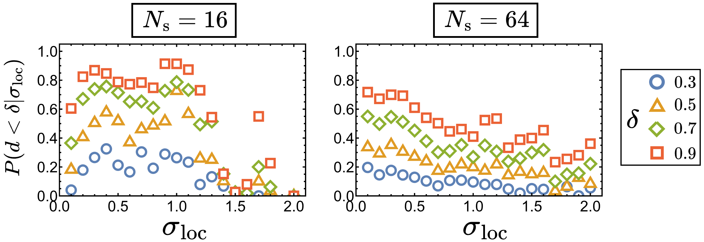
Figure 4: Same as Fig. 3 but computed using the models which ranked first with the overlap criterion discussed in Sec. II.3.

Remarkably, this would no longer hold if we used only the model with the largest overlap integral $\mathcal{Z}$ to infer the source location. Indeed, in such a case, the correlation between the distance from the true source location and its uncertainty almost disappears, with the outcome comparable to the one of the SMC algorithm, compare Fig. 4 with the top panels of Fig. 3. This emphasizes the importance of blending information from many wrong models to estimate the source location, as done in the WBU approach.

III.2 Model misspecification: the effect of correlations

Although WBU and SMC use both the same (wrong) model of the environment to infer the source location, they have different outcomes, with the former proving to be less sensitive to the model misspecification than the latter. It is, therefore, worth investigating more systematically how model errors affect the performance of such source localization algorithms. As shown in the table in Fig. 5(a), we can consider four possible ways to infer the source location with a given algorithm when dealing with realistic data of turbulent odor dispersion.

The first possibility is to use the Lagrangian time series obtained from the DNS to determine whether a sensor detects an odor or not and then deploy a (inevitably misspecified) model of the environment —like the one derived from Eq. (3)— to interpret such detections and compute the likelihood (Model likelihood-Correlated signal —MlCs— top left cell in the table). This is precisely the scenario we have analyzed so far, which is the closest one to reality as it relies on minimal prior knowledge of the environment and directly uses the Lagrangian data.

Alternatively, as a model of the environment, we can use the empirical likelihood [Fig. 1(b)] computed from the time history of all the odor trajectories obtained from the DNS. On the one hand, this approach [Empirical likelihood-Correlated signal —ElCs— bottom left cell in the table in Fig. 5(a)] greatly simplifies the search since there are no environmental parameters to fit, and it also represents the best existing (empirical) model one can aim for in practice to infer the source location. On the other hand, however, it is still an imperfect model of the environment as it does not capture the time and spatial correlations featured by the odor plume [12].

To study how such correlations affect the source position estimation, we should then consider the case where the detections are not directly taken from the DNS time series but instead randomly drawn from the empirical likelihood. Indeed, the sensors’ measurements are in this way uncorrelated while still featuring the same detection statistics as the original signal. At this point, we can decide whether to deploy the empirical likelihood itself to infer the source location, in which case we would be using the exact model of the environment (Empirical likelihood-Uncorrelated signal —ElUs— bottom right cell in the table) or the usual probabilistic model of detections (Model likelihood-Uncorrelated signal —MlUs— top right cell in the table). The former can be helpful as a benchmark since, provided the number of measurements is large enough, it should show convergence to the correct solution for any properly implemented localization algorithm based on Bayesian inference. The latter is instead useful compared to the first two cases illustrated above since, in this case, sensors’ observations are uncorrelated and, as a result, it isolates the effect of dealing with a functionally wrong model of the environment.

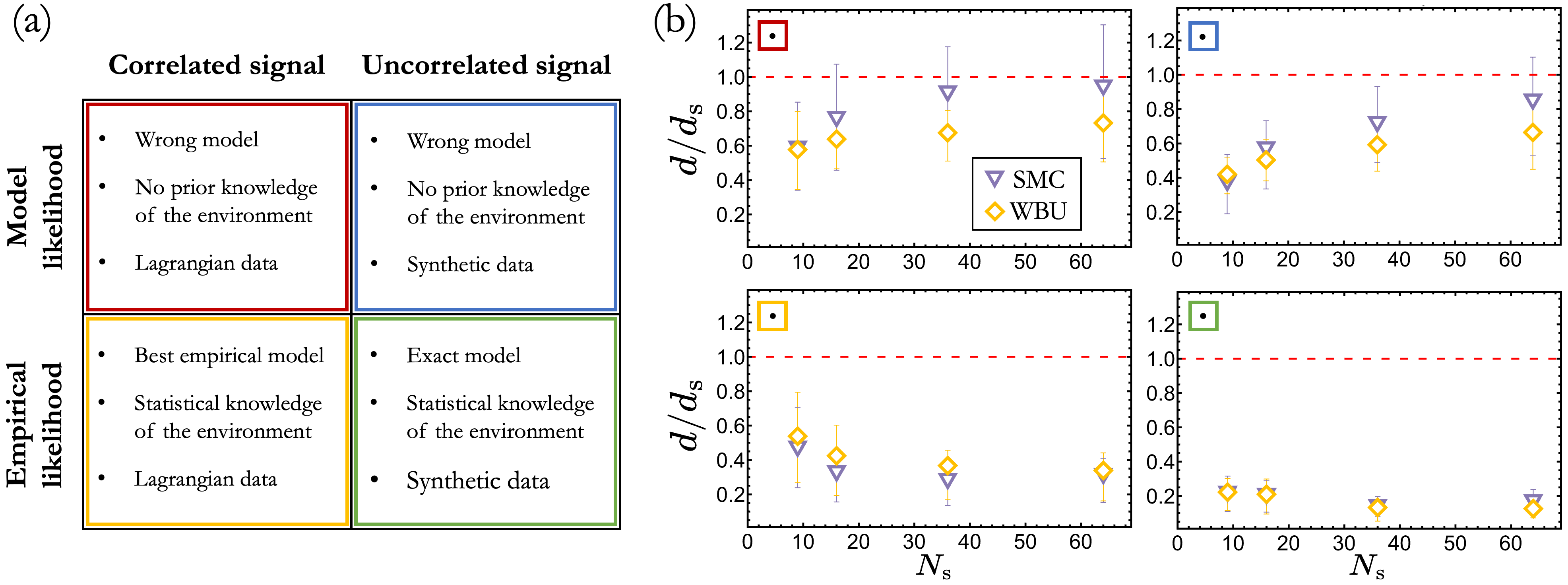
Figure 5: (a) Table summarizing all the possible ways to infer the source location when dealing with realistic data of turbulent odor dispersion. They may differ for the model used to compute the likelihood (rows) or for the signal received by the sensors (columns). (b) Mean distance $d$ from the source at the end of each episode in units of the distance $d_{\rm{s}}$ between sensors as a function of the number of sensors $N_{\rm s}$. Different symbols correspond to the algorithm employed (SMC: inverted purple triangles; WBU: yellow diamonds). Error bars are the first and third quartiles of the distribution. Each plot refers to one of the four cases illustrated in table (a), as indicated by the box color in the upper left corner.

This completes the picture in the table in Fig. 5(a). We are now ready to compare the performance of WBU and SMC in each of the four scenarios just described. To this end, we shall look at the results reported in Fig. 5(b). There, we show the average distance $d$ between the actual source location and its estimate given by either algorithm at the end of distinct episodes of set time length as a function of the number of sensors $N_{\rm s}$ deployed in the search (details in Appendix B). Some observations are in order. First of all, both WBU (yellow diamonds) and SMC (purple inverted triangles) show comparable performance as long as they use the empirical likelihood to model the detection statistics (plots in the bottom row). More specifically, when using the exact model as in the ElUs scenario, both approaches tend to converge to the correct source location as expected (bottom right plot). At the same time, by looking at the ElCs case (bottom left plot), we may observe how much the sole presence of time and spatial correlations in the signal affects the quality of the source estimate. Remarkably, even though the empirical model does not account for such correlations, both algorithms manage to locate the source within a distance $d$ smaller than half of the sensor separation.

Now, let us see what changes when using the probabilistic model introduced in Sec. II.2 to infer the source location (MlCs and MlUs scenarios —plots in the top row). While using the wrong model has obvious shortcomings and further degrades the performance of both approaches, overall, they prove to be quite robust and still manage, on average, to locate the source within a distance smaller than the one between sensors. Furthermore, comparing the results obtained with uncorrelated signals (MlUs, top right plot) with the most realistic scenario featuring the correlated signal (MlCs, top left plot), we may notice that the SMC’s performance gets substantially worse in the latter case, while WBU is basically unaffected.

The higher sensitivity of SMC to correlations can be rationalized by looking at the time evolution of the model parameters, namely the emission rate $Q$ and the characteristic length scale of turbulent odor dispersion $\lambda$, inferred by such an algorithm. As shown in Fig. 6, when the signal received by the sensors is correlated in space and time (blue curves), SMC has the tendency to overestimate both $\lambda$ and $Q$, even saturating to the maximum allowed value. The picture dramatically changes when the sensors’ observations are instead uncorrelated (orange curves). There, the inferred values of the parameters are much closer to the ones obtained from the best fit of the empirical likelihood (dashed red line in both plots), which means the algorithm is, in this case, pointing in the right direction.

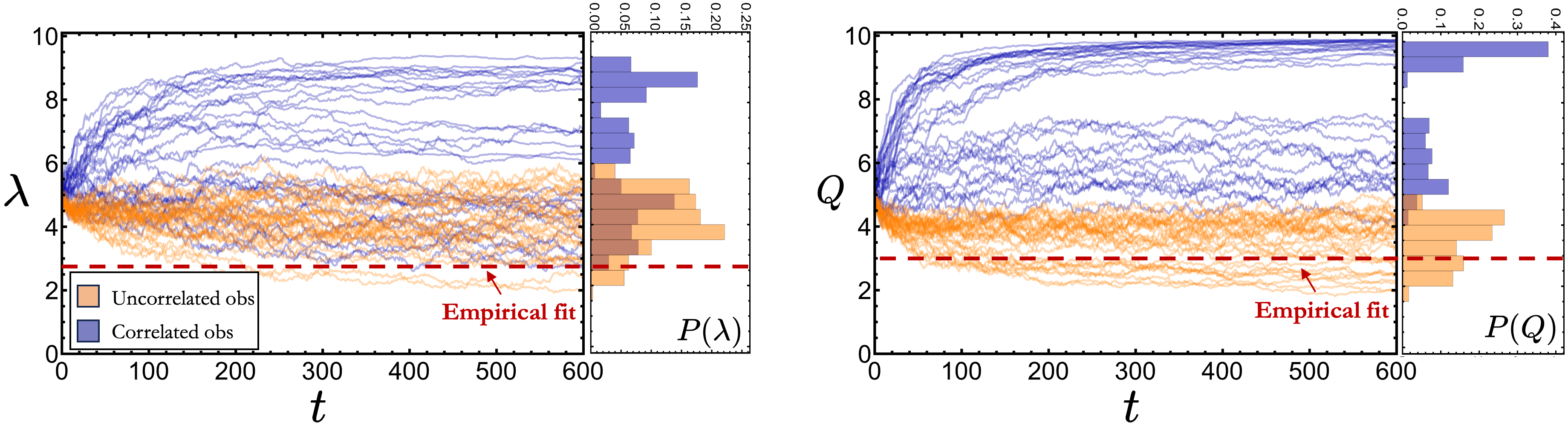
Figure 6: Comparison between the values of the model parameters (left: $\lambda$; right: $Q$) inferred by the SMC algorithm as a function of time when directly using the DNS time series (blue curves, time-correlated signal) and when extracting the detections from the corresponding empirical likelihood (orange curves, uncorrelated signal). In both cases, each curve corresponds to the episodes-averaged value of the parameter obtained in one of the $30$ configurations (different source positions) where the algorithm has been tested. The histograms on the right of each plot have been obtained by considering the inferred values of the parameters at times $t\geq 300$, while the horizontal dashed red lines stand for the values of $\lambda$ and $Q$ derived from the best fit of the empirical likelihood. Data shown here correspond to the setup with $N_{\rm s}=16$ sensors.

Hence, the observed sensitivity of the SMC algorithm in the most realistic scenario lies in the fact that it must perform a real-time inference of the model parameters (while looking for the source), which is greatly impacted by the presence of time correlations in the signal. However, this is not the case for the WBU approach since it uses a predetermined and discrete set of parameters, then runs the different models independently, and only at the end merges their outcome based on the current ranking provided by the overlap integral of each model. The static nature of the parameter space and the use of all available (misspecified) models are thus the defining strengths of the newly introduced approach.

IV Discussion

In this work, we revisited the problem of locating an odor source in a realistic turbulent environment with a network of static sensors. To this end, we employed DNS of the incompressible 3–D Navier-Stokes equations to simulate odor dispersion in the atmospherical boundary layer. We then used the data of the Lagrangian particles trajectories to systematically investigate how the errors made in modeling such an environment, a problem unavoidable in field applications, affect the performance of source localization algorithms based on Bayesian inference.

Within this framework, we identified a quantity that effectively ranks different models of the environment just based on the history of observations made by the sensors in the field. This is what we called the overlap integral $\mathcal{Z}$ as it essentially measures the degree of consensus among the sensors about a single source location. This quantity, which is maximized when the model is exact, also represents the posterior estimate of the probability of making the sequence of observations, integrated over all possible source locations. Thus, our weighted Bayesian update (WBU) approach to source localization may be viewed as a form of maximum likelihood estimation (MLE) applied to the model itself. The use of MLE to quantify the degree of model misspecification was previously studied in an abstract setting in Ref. [52].

Through our analysis, we may conclude that WBU is a more robust approach to locating an odor source in a turbulent environment than state-of-the-art methods relying on Monte Carlo sampling techniques. In fact, our results highlight some fundamental weaknesses of the Sequential Monte Carlo (SMC) algorithm, which features a strong sensitivity to the presence of time/space correlations in the sensors’ detections, especially in the most general case where it must also infer the model parameters in real-time together with the source location. This is in contrast with WBU, which is insensitive to correlations and proved to be only mildly affected by the use of wrong models. In particular, WBU, as opposed to SMC, is able to maintain the desired correlation between the uncertainty about the source location and the distance of its current estimate from the ground truth. Thus, WBU provides a robust stop criterion for the search.

The main novelty of the WBU approach stems from the idea that merging the information gathered from many possible interpretations of the measurements recorded by the sensors may help in compensating for model errors consistently with the many wrongs principle [33, 34]. In the realm of olfactory search, this represents a fundamental stepping stone toward a thorough investigation of the effect of misspecified models on the localization of odor sources in turbulent environments, an unavoidable difficulty in practical applications.

The presented results and methodology have clear potential applications in environmental monitoring [28, 53] and early warnings [29], as they allow to reliably identify a potential area of intervention when some hazardous substances are detected. It would also be interesting to explore the possibility of capitalizing on the use of many wrong models in the case of olfactory search by single [18, 20] or multiple [19] moving agents, where it can help mitigate the model misspecification and thus allow for better decisions of the agent(s). Beyond olfactory search, the WBU approach is, in principle, also adaptable to any other Bayesian inference problem with model misspecification. Finally, we suggest that the overlap integral could be maximized instead by gradient ascent, which would afford a reduction in computational cost and memory load while losing the extra information from running many wrong models. It would be interesting, in particular, to explore the use of a powerful, many-parameter model such as a neural network in such a context.

Appendix A Analytical argument for the convergence of the overlap integral

Let the true likelihood be $f(h|\bm{r}_{i}-\bm{r})$ and let Bayesian updates be performed with a model $g(h|\bm{r}_{i}-\bm{r}),$ not necessarily correctly specified. Let the prior be $\pi(\bm{r}),$ and let the true source location be $\bm{r}^{*}.$

After $T$ timesteps, we have

$$\mathcal{Z}=\int_{\Omega}d\bm{r}\,\pi(\bm{r})\prod_{i=1}^{N_{s}}\prod_{t=1}^{T}g(h_{i}^{(t)}|\bm{r}_{i}-\bm{r})=\int_{\Omega}d\bm{r}\,\pi(\bm{r})\exp\left(\sum_{i=1}^{N_{s}}\sum_{t=1}^{T}\log g(h_{i}^{(t)}|\bm{r}_{i}-\bm{r})\right).$$ (A1)

As long as each observation $h_{i}^{(t)}$ has bounded variance and correlations between observations decay to zero over time (i.e. $\mathrm{Cov}(h^{(t)},h^{(t+\tau)})\xrightarrow{\tau\to\infty}0$), we may apply the (weak) law of large numbers [54], which implies that the argument of the exponential converges in probability to its expectation over observations $h$:

$$\mathcal{Z} \to\bar{\mathcal{Z}}_{T}\equiv\int_{\Omega}d\bm{r}\,\pi(\bm{r})\exp\left(T\sum_{i=1}^{N_{s}}\sum_{h\in\{0,1\}}f(h|\bm{r}_{i}-\bm{r}^{*})\log g(h|\bm{r}_{i}-\bm{r})\right)$$

$$=C_{T}\int_{\Omega}d\bm{r}\,\pi(\bm{r})\exp\left[-T\sum_{i=1}^{N_{s}}D_{\rm KL}(f(\cdot|\bm{r}_{i}-\bm{r}^{*})\parallel g(\cdot|\bm{r}_{i}-\bm{r}))\right],$$ (A2)

where

$$C_{T}=\exp\left(-T\sum_{i=1}^{N_{s}}H(f(\cdot|\bm{r}_{i}-\bm{r}^{*}))\right),$$ (A3)

$D_{\rm KL}(p\parallel q)$ indicates the Kullback-Leibler divergence between distributions $p$ and $q,$ and $H$ is the Shannon entropy. By Gibbs’ inequality,

$$F(\bm{r})\equiv\sum_{i=1}^{N_{s}}D_{\rm KL}(f(\cdot|\bm{r}_{i}-\bm{r}^{*})\parallel g(\cdot|\bm{r}_{i}-\bm{r}))\geq 0,$$ (A4)

with equality iff $f(h|\bm{r}_{i}-\bm{r}^{*})=g(h|\bm{r}_{i}-\bm{r})$ for each $1\leq i\leq N_{s}$ and each $0\leq h\leq N_{o}-1$ (where $N_{o}$ is the number of possible observations, which we have set to two). The set of points $\bm{r}$ where this holds is the intersection of $N_{s}\times N_{o}$ manifolds of codimension 1; assuming $f$ and $g$ are well-behaved functions of position, for large enough $N_{s}$ this intersection should be empty unless $f(h|\bm{r}_{i}-\bm{r}^{*})=g(h|\bm{r}_{i}-\bm{r}^{*})$ for each $i$ and $h$, in which case the unique member will be the point $\bm{r}=\bm{r}^{*}.$

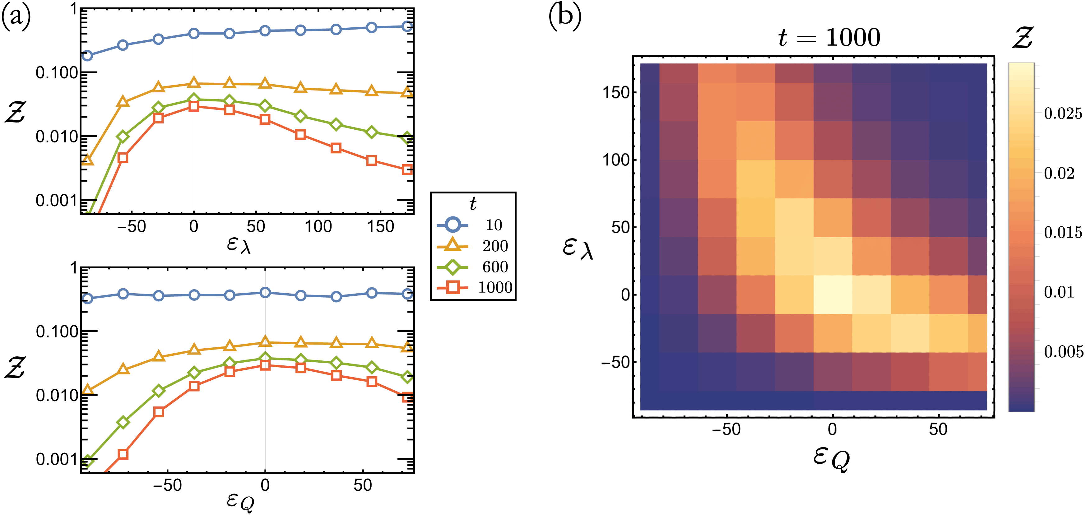
Figure A1: (a) Curves of the overlap integral $\mathcal{Z}$ as a function of the percentage error on either of the model parameters. Different curves refer to distinct times, as indicated in the legend. (b) Colormap of the overlap integral $\mathcal{Z}$ at time $t=10^{3}$ as a function of the percentage error on both model parameters. As expected, it features a maximum when the model is exact ($\varepsilon_{\lambda}=\varepsilon_{Q}=0$) and decays to zero as we move away from it. Data shown here have been obtained by averaging over $10^{2}$ episodes of time length $T=10^{3}$ in units of observations made by each sensor.

Since $T$ is large, Laplace’s method gives

$$\bar{\mathcal{Z}}_{T}\sim T^{-d/2}C_{T}\sum_{j=1}^{k}a_{j}\exp(-TF(\hat{\bm{r}}_{j}))=T^{-d/2}C_{T}\exp(-T\hat{F})\sum_{j=1}^{k}a_{j},$$ (A5)

where $d$ is the number of spatial dimensions, $\hat{F}$ is the minimum of $F$ and is attained on the set $\{\hat{\bm{r}}_{j}\}_{j=1}^{k},$ and each $a_{j}$ is nonnegative and independent of $T.$ Therefore, $\bar{\mathcal{Z}}_{T}$ is maximized when $f$ and $g$ agree at each $\bm{r}_{i}-\bm{r}^{*}$ and is exponentially smaller when they do not. This is the key result.

We can numerically show that the overlap integral $\mathcal{Z}$ relaxes to zero faster the farther from the ground truth the model is. To this end, let us take into account the same setup as the one shown in Fig. 2, with the source located in $\bm{r}_{\rm s}=(92,70)$ and $N_{\rm s}=16$ sensors placed on a square lattice tilted by an angle $\theta=1.04\,\rm{rad}$ with respect to the wind direction. We can then use the probabilistic model described in Sec. II.2 to generate the observations made by the static sensors and set the source emission rate and the characteristic length scale of the turbulent odor dispersion to $Q^{*}=5.5$ and $\lambda^{*}=3.5$, respectively. Since we know the exact model of the detection statistics, we can systematically study how the overlap integral $\mathcal{Z}$ varies depending on the error made on such model parameters. Figure A1(a) shows the values of $\mathcal{Z}$ obtained when either the value of the characteristic length scale $\lambda$ (top panel) or the one of the emission rate $Q$ (bottom panel) is wrong. In both cases, as time progresses, the curve of the overlap integral peaks more and more around the correct value of the parameter, i.e., the one corresponding to a percentage error $\varepsilon_{*}=0$, and it smoothly goes to zero as the error grows. More generally, this still holds when both model parameters are misspecified, as shown in the colormap in Fig. A1(b).

Let us now comment on one feature that stands out from these plots, that is, the observed asymmetry in the values of $\mathcal{Z}$ when $\lambda$ is under/over-estimated. In fact, given the same history of measurements, the source will be estimated as farther from the sensors, the greater the estimated value of $\lambda$. This will eventually cause the overlap among the private beliefs to accumulate at the border of the finite-size arena $\Omega$ where simulations are performed. Therefore, the larger values of the overlap integral $\mathcal{Z}$ when $\lambda$ is overestimated are a mere finite-size effect. On the one hand, this is not a problem in the case of a functionally correct model, where the ground truth is attainable (as in this section) since, eventually, the correct model will still be the one with the largest value of $\mathcal{Z}$ anyway. On the other hand, however, this effect can persist in the general case of a functionally wrong model (scenario discussed in the main text), and we are compelled to address it for consistency. To this end, during our analysis, we systematically set to zero the values of the overlap for the models that would place the source at a distance $d\leq 5\Delta x$ (with $\Delta x$ being the lattice spacing) from the border of the arena $\Omega$. This avoids the selection of clearly wrong models that only artificially would feature a large value of the overlap $\mathcal{Z}$, preserving the structure and the basic concepts behind the WBU approach.

Appendix B Details on the numerical simulations

In all our numerical simulations, the size of the square arena $\Omega$ has been set to $128\Delta x\times 128\Delta x$, with $\Delta x=1$ being the lattice spacing. The sensors have been placed in a square lattice of side $\ell=88\Delta x$, tilted with an angle $\theta=1.04$ with respect to the mean wind direction. All the data presented in Sec. III have then been obtained by averaging over the results obtained by shifting the odor source in $30$ different locations drawn at random within an inner box $108\Delta x\times 108\Delta x$ inside $\Omega$, as illustrated in Fig. A2. This was done to avoid boundary effects that would have altered the performance statistics of the localization algorithms.

Moreover, to gather more statistics for each source location, we have divided the time series of the odor dispersion obtained from the DNS described in Sec. II.1 into $25$ runs of set time length $T=600$ (in units of the Kolmogorov timescale $\tau_{\eta}$).

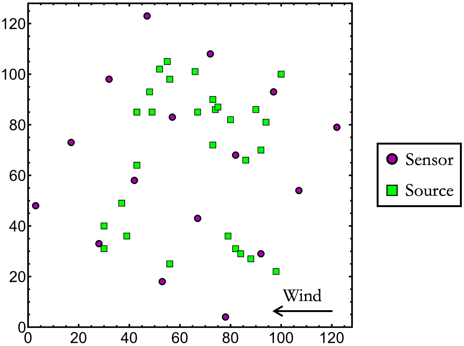
Figure A2: Illustration of the sensors’ placement (magenta circles, here $N_{\rm s}=16$) and of the $30$ source locations (green squares) drawn at random inside the arena.

Definition	Symbol	Value
Number of samples	$N$	50
Number of MCMC perturbation steps	$K$	5
Variance of proposal distribution of $\bm{r}_{\rm s}$	$\sigma^{2}_{\rm pos}$	100
Variance of proposal distribution of $\lambda$	$\sigma^{2}_{\lambda}$	1
Variance of proposal distribution of $Q$	$\sigma^{2}_{Q}$	1
Range of values of $\lambda$	$[\lambda_{\rm m},\lambda_{\rm M}]$	[0,10]
Range of values of $Q$	$[Q_{\rm m},Q_{\rm M}]$	[0,10]

Table A1: Values of the hyperparameters used in the SMC algorithm.

In order to get the master belief in the WBU approach, we have used in every configuration a total of $M=100$ models, each of them corresponding to a different combination of parameters $\{Q,\lambda\}$ in the stochastic model introduced in Sec. II.2, with the specific values of $Q$ and $\lambda$ being $Q=\{0.7,1.7,\dots,9.7\}$ and $\lambda=\{0.7,1.7,\dots,9.7\}$, respectively.

The values of the SMC hyperparameters used in this work are summarized in Table A1. We have also numerically checked that all the results presented here are not qualitatively affected by this choice. Note that, in the SMC implementation, we start from a flat prior defined over the interval $[0;10]$ for both model parameters $Q$ and $\lambda$. Moreover, their values are bounded therein, which is, for consistency, the same range used in the WBU approach.

Lastly, the detailed step-by-step explanation of the WBU and SMC implementation is reported in Algorithm 1 and Algorithm 2, respectively.

Algorithm 1 Weighted Bayesian update

1:for $j=1$ to $M$ do $\triangleright$ Loop over different models

2:     Set initial common belief $B^{(0)}_{j}$ to a uniform distribution.

3:     Set model parameters $\bm{P}_{j}=\{Q_{j},\lambda_{j}\}$.

4:     for $t=1$ to $T$ do $\triangleright$ Loop over time

5:         Perform sensors’ measurements $\bm{h}^{(t)}$.

6:         Update common belief $B^{(t)}_{j}$ using Bayes’ rule (10).

7:         Compute overlap integral $\mathcal{Z}^{(t)}_{j}$.

8:     end for

9:end for

10:Compute master belief $\mathcal{B}_{M}$ at all times from Eq. (11). $\triangleright$ Output master belief from weighted models

Algorithm 2 Sequential Monte Carlo with Importance Sampling and perturbation step

1:Set initial belief $\tilde{B}^{(0)}$ to a uniform distribution.

2:for $t=1$ to $T$ do

3:     Perform sensors’ measurements $\bm{h}^{(t)}$.

4:     for $i=1$ to $N$ do $\triangleright$ Sample’s initialization

5:         Draw sample from current belief: $\tilde{\bm{\theta}}_{i}\sim\tilde{B}^{(t-1)}(\bm{\theta})$.

6:         Compute weight $w_{i}=\mathcal{L}(\bm{h}^{(t)}|\tilde{\bm{\theta}}_{i})$.

7:     end for

8:     for $i=1$ to $N$ do

9:         Normalize weight: $w_{i}/=\sum_{i=1}^{N}w_{i}$.

10:         Compute Effective Sample Size: $N_{{\rm eff}}=1/\sum_{i=1}^{N}w_{i}^{2}$.

11:     end for

12:     if $N_{\text{eff}}<N_{\text{thr}}$ then $\triangleright$ Resampling step (if needed)

13:         for $i=1$ to $N$ do

14:              Select $\tilde{\bm{\theta}}_{k}$ with probability $w_{k}$.

15:              Put $\tilde{\bm{\Theta}}_{i}=\tilde{\bm{\theta}}_{k}$.

16:         end for

17:         for $i=1$ to $N$ do

18:              Replace $\tilde{\bm{\theta}}_{i}=\tilde{\bm{\Theta}}_{i}$.

19:              Set uniform weights: $w_{i}=1/N$.

20:         end for

21:     end if

22:     for $i=1$ to $N$ do $\triangleright$ MCMC perturbation step

23:         Select $l\in\{1,\dots,N\}$ with probability $w_{l}$.

24:         Set $\bm{\theta}^{(t)}_{i,0}=\tilde{\bm{\theta}}^{(t)}_{l}$.

25:         for $j=1$ to $K$ do

26:              Draw new sample from proposal distribution: $\hat{\bm{\theta}}^{(t)}\sim q(\hat{\bm{\theta}}^{(t)}|\bm{\theta}^{(t)}_{i,j-1})$.

27:              Compute acceptance ratio $\alpha$ from Eq. (12).

28:              Draw random number $u\sim U[0,1]$.

29:              if $u<\min(1,\alpha)$ then

30:                  Set $\bm{\theta}^{(t)}_{i,j}=\hat{\bm{\theta}}^{(t)}$.

31:              else

32:                  Set $\bm{\theta}^{(t)}_{i,j}=\bm{\theta}^{(t)}_{i,j-1}$.

33:              end if

34:         end for

35:         Set $\bm{\theta}^{(t)}_{i}=\bm{\theta}^{(t)}_{i,\tilde{B}}$.

36:     end for

37:     Set $\tilde{B}^{(t)}(\bm{\theta})=1/N\sum_{i=1}^{N}\delta(\bm{\theta}-\bm{\theta}^{(t)}_{i})$. $\triangleright$ Output belief approximation

38:end for

References

- Bayat et al. [2017] B. Bayat, N. Crasta, A. Crespi, A. M. Pascoal, and A. Ijspeert, Environmental monitoring using autonomous vehicles: a survey of recent searching techniques, Curr. Opin. Biotechnol. 45, 76 (2017).
- Burgués and Marco [2020] J. Burgués and S. Marco, Environmental chemical sensing using small drones: A review, Sci. Total Environ. 748, 141172 (2020).
- Francis et al. [2022] A. Francis, S. Li, C. Griffiths, and J. Sienz, Gas source localization and mapping with mobile robots: A review, J. Field Robot. 39, 1341 (2022).
- Karafasoulis and Kyriakis [2023] K. Karafasoulis and A. Kyriakis, Spatial localization of radioactive sources for homeland security, in Gamma Ray Imaging: Technology and Applications, edited by J. Du and K. K. Iniewski (Springer International Publishing, Cham, 2023) pp. 87–102.
- Murlis et al. [1992] J. Murlis, J. S. Elkinton, and R. T. Cardé, Odor plumes and how insects use them, Annu. Rev. Entomol. 37, 505 (1992).
- Hein et al. [2016] A. M. Hein, F. Carrara, D. R. Brumley, R. Stocker, and S. A. Levin, Natural search algorithms as a bridge between organisms, evolution, and ecology, Proc. Natl. Acad. Sci. 113, 9413 (2016).
- Aref et al. [2017] H. Aref, J. R. Blake, M. Budišić, S. S. S. Cardoso, J. H. E. Cartwright, H. J. H. Clercx, K. El Omari, U. Feudel, R. Golestanian, E. Gouillart, G. F. van Heijst, T. S. Krasnopolskaya, Y. Le Guer, R. S. MacKay, V. V. Meleshko, G. Metcalfe, I. Mezić, A. P. S. de Moura, O. Piro, M. F. M. Speetjens, R. Sturman, J.-L. Thiffeault, and I. Tuval, Frontiers of chaotic advection, Rev. Mod. Phys. 89, 025007 (2017).
- Speetjens et al. [2021] M. Speetjens, G. Metcalfe, and M. Rudman, Lagrangian Transport and Chaotic Advection in Three-Dimensional Laminar Flows, Appl. Mech. Rev. 73, 030801 (2021).
- Frisch [1995] U. Frisch, Turbulence: The Legacy of A. N. Kolmogorov (Cambridge University Press, 1995).
- Alexakis and Biferale [2018] A. Alexakis and L. Biferale, Cascades and transitions in turbulent flows, Phys. Rep. 767-769, 1 (2018), cascades and transitions in turbulent flows.
- Crimaldi and Koseff [2001] J. P. Crimaldi and J. R. Koseff, High-resolution measurements of the spatial and temporal scalar structure of a turbulent plume, Exp. Fluids 31, 90 (2001).
- Celani et al. [2014] A. Celani, E. Villermaux, and M. Vergassola, Odor landscapes in turbulent environments, Phys. Rev. X 4, 041015 (2014).
- Piro [2023] L. Piro, Optimal navigation in active matter, Ph.D. thesis, Georg-August-Universität Göttingen Göttingen (2023).
- Reddy et al. [2022] G. Reddy, V. N. Murthy, and M. Vergassola, Olfactory sensing and navigation in turbulent environments, Annu. Rev. Condens. Matter Phys. 13, 191 (2022).
- Belanger and Willis [1998] J. Belanger and M. Willis, Biologically-inspired search algorithms for locating unseen odor sources, in Proc. 1998 IEEE International Symposium on Intelligent Control (ISIC) held jointly with IEEE International Symposium on Computational Intelligence in Robotics and Automation (CIRA) Intell (1998) pp. 265–270.
- Balkovsky and Shraiman [2002] E. Balkovsky and B. I. Shraiman, Olfactory search at high reynolds number, Proc. Natl. Acad. Sci. 99, 12589 (2002), https://www.pnas.org/doi/pdf/10.1073/pnas.192393499 .
- Durve et al. [2020] M. Durve, L. Piro, M. Cencini, L. Biferale, and A. Celani, Collective olfactory search in a turbulent environment, Phys. Rev. E 102, 012402 (2020).
- Vergassola et al. [2007] M. Vergassola, E. Villermaux, and B. I. Shraiman, ‘Infotaxis’ as a strategy for searching without gradients, Nature 445, 406 (2007).
- Masson et al. [2009] J.-B. Masson, M. B. Bechet, and M. Vergassola, Chasing information to search in random environments, J. Phys. A-Math. Theor. 42, 434009 (2009).
- Loisy and Eloy [2022] A. Loisy and C. Eloy, Searching for a source without gradients: how good is infotaxis and how to beat it, Proc. R. Soc. A 478, 20220118 (2022), https://royalsocietypublishing.org/doi/pdf/10.1098/rspa.2022.0118 .
- Keats et al. [2007] A. Keats, E. Yee, and F.-S. Lien, Bayesian inference for source determination with applications to a complex urban environment, Atmos. Environ. 41, 465 (2007).
- Hutchinson et al. [2019] M. Hutchinson, C. Liu, and W.-H. Chen, Source term estimation of a hazardous airborne release using an unmanned aerial vehicle, J. Field Robot. 36, 797 (2019), https://onlinelibrary.wiley.com/doi/pdf/10.1002/rob.21844 .
- Aslam et al. [2003] J. Aslam, Z. Butler, F. Constantin, V. Crespi, G. Cybenko, and D. Rus, Tracking a moving object with a binary sensor network, in Proc. of the 1st International Conference on Embedded Networked Sensor Systems, SenSys ’03 (Association for Computing Machinery, New York, NY, USA, 2003) p. 150–161.
- Shankar Rao [2007] K. Shankar Rao, Source estimation methods for atmospheric dispersion, Atmos. Environ. 41, 6964 (2007).
- Hutchinson et al. [2017] M. Hutchinson, H. Oh, and W.-H. Chen, A review of source term estimation methods for atmospheric dispersion events using static or mobile sensors, Inform. Fusion 36, 130 (2017).
- Sättele et al. [2015] M. Sättele, M. Bründl, and D. Straub, Reliability and effectiveness of early warning systems for natural hazards: Concept and application to debris flow warning, Reliab. Eng. Syst. Saf. 142, 192 (2015).
- Stähli et al. [2015] M. Stähli, M. Sättele, C. Huggel, B. W. McArdell, P. Lehmann, A. Van Herwijnen, A. Berne, M. Schleiss, A. Ferrari, A. Kos, D. Or, and S. M. Springman, Monitoring and prediction in early warning systems for rapid mass movements, Nat. Hazards Earth Syst. Sci. 15, 905 (2015).
- Tariq et al. [2021] S. Tariq, Z. Hu, and T. Zayed, Micro-electromechanical systems-based technologies for leak detection and localization in water supply networks: A bibliometric and systematic review, J. Clean. Prod. 289, 125751 (2021).
- Esposito et al. [2022] M. Esposito, L. Palma, A. Belli, L. Sabbatini, and P. Pierleoni, Recent advances in internet of things solutions for early warning systems: A review, Sensors 22, 10.3390/s22062124 (2022).
- Platt and DeRiggi [2012] N. Platt and D. DeRiggi, Comparative investigation of source term estimation algorithms using fusion field trial 2007 data: linear regression analysis, Int. J. Environ. Pollut. 48, 13 (2012), https://www.inderscienceonline.com/doi/pdf/10.1504/IJEP.2012.049647 .
- Berk [1966] R. H. Berk, Limiting behavior of posterior distributions when the model is incorrect, Ann. Math. Stat. 37, 51 (1966).
- Berk [1970] R. H. Berk, Consistency a posteriori, Ann. Math. Stat. 41, 894 (1970).
- Simons [2004] A. Simons, Many wrongs: The advantage of group navigation, Trends Ecol. Evol. 19, 453–455 (2004).
- Berdahl et al. [2018] A. M. Berdahl, A. B. Kao, A. Flack, P. A. H. Westley, E. A. Codling, I. D. Couzin, A. I. Dell, and D. Biro, Collective animal navigation and migratory culture: from theoretical models to empirical evidence, Philos. Trans. R. Soc. Lond. B Biol. Sci. 373, 20170009 (2018), https://royalsocietypublishing.org/doi/pdf/10.1098/rstb.2017.0009 .
- Doucet et al. [2000] A. Doucet, S. Godsill, and C. Andrieu, On sequential Monte Carlo sampling methods for Bayesian filtering, Stat. Comput. 10, 197 (2000).
- Sawford [1991] B. Sawford, Reynolds number effects in lagrangian stochastic models of turbulent dispersion, Phys. Fluids A: Fluid Dyn. 3, 1577 (1991).
- Holmes and Morawska [2006] N. Holmes and L. Morawska, A review of dispersion modelling and its application to the dispersion of particles: An overview of different dispersion models available, Atmos. Environ. 40, 5902 (2006).
- Falkovich et al. [2001] G. Falkovich, K. Gawȩdzki, and M. Vergassola, Particles and fields in fluid turbulence, Rev. Mod. Phys. 73, 913 (2001).
- Biferale et al. [1995] L. Biferale, A. Crisanti, M. Vergassola, and A. Vulpiani, Eddy diffusivities in scalar transport, Phys. Fluids 7, 2725 (1995).
- Ristic et al. [2016] B. Ristic, A. Gunatilaka, and R. Gailis, Localisation of a source of hazardous substance dispersion using binary measurements, Atmos. Environ. 142, 114 (2016).
- Smoluchowski [1918] M. v. Smoluchowski, Versuch einer mathematischen theorie der koagulationskinetik kolloider lösungen, Z. Phys. Chem. 92, 129 (1918).
- Box and Tiao [2011] G. E. Box and G. C. Tiao, Bayesian inference in statistical analysis (John Wiley & Sons, 2011).
- Schwartz [1965] L. Schwartz, On Bayes procedures, Zeitschrift für Wahrscheinlichkeitstheorie und Verwandte Gebiete 4, 10 (1965).
- Fishman [1996] G. S. Fishman, Monte Carlo: Concepts, Algorithms and Applications (Springer Verlag, New York, NY, USA, 1996).
- Johannesson et al. [2004] G. Johannesson, B. Hanley, and J. Nitao, Dynamic Bayesian Models via Monte Carlo - An Introduction with Examples -, Tech. Rep. (U.S. Department of Energy Office of Scientific and Technical Information, 2004).
- Elfring et al. [2021] J. Elfring, E. Torta, and R. van de Molengraft, Particle filters: A hands-on tutorial, Sensors 21, 10.3390/s21020438 (2021).
- Metropolis et al. [1953] N. Metropolis, A. W. Rosenbluth, M. N. Rosenbluth, A. H. Teller, and E. Teller, Equation of State Calculations by Fast Computing Machines, J. Chem. Phys. 21, 1087 (1953).
- Musso et al. [2001] C. Musso, N. Oudjane, and F. Le Gland, Improving regularised particle filters, in Sequential Monte Carlo Methods in Practice, edited by A. Doucet, N. de Freitas, and N. Gordon (Springer New York, New York, NY, 2001) pp. 247–271.
- Thomson et al. [2007] L. C. Thomson, B. Hirst, G. Gibson, S. Gillespie, P. Jonathan, K. D. Skeldon, and M. J. Padgett, An improved algorithm for locating a gas source using inverse methods, Atmos. Environ. 41, 1128 (2007).
- Ristic et al. [2015] B. Ristic, A. Gunatilaka, and R. Gailis, Achievable accuracy in gaussian plume parameter estimation using a network of binary sensors, Inform. Fusion 25, 42 (2015).
- Note [1] Clearly, the and counterparts in the SMC algorithm are respectively defined as the variance and mean computed over the Monte Carlo samples.
- White [1982] H. White, Maximum likelihood estimation of misspecified models, Econometrica 50, 1 (1982).
- Ullo and Sinha [2020] S. L. Ullo and G. R. Sinha, Advances in smart environment monitoring systems using iot and sensors, Sensors 20, 10.3390/s20113113 (2020).
- Bernshtein [1918] S. N. Bernshtein, Sur la loi des grands nombres, Communications de la Société mathématique de Kharkow 16, 82 (1918).