Diphoton signals for the Georgi-Machacek scenario at the Large Hadron Collider

Abstract

The diphoton channel for exploring the Georgi-Machacek (GM) scenario containing scalar triplets at the Large Hadron Collider (LHC) has been identified as germane, and subjected to a detailed study. The scalar spectrum of the model, which imposes a custodial SU(2) on the potential, gets classified into a 5-plet, a 3-plet and two singlets under the custodial symmetry. While most attempts to probe or constrain the scenario at the LHC depend largely on signals of charged scalars, we point out that the custodial SU(2) singlet state H can have a substantial branching ratio (amounting to a few per cent) into two photons. We carry out a detailed simulation of the resulting signal and the standard model backgrounds, obtaining the signal significance in different regions of the parameter space using the profile likelihood ratio method. Substantial regions of the GM parameter space is thus shown to be accessible to LHC studies, both at the high-luminosity run with $\int{\cal L}dt=3000fb^{-1}$, and also in Run-3 with $\int{\cal L}dt=300fb^{-1}$, even after folding in systematic errors.

1 Introduction

Scenarios where electroweak symmetry is broken by the vacuum expectation values (vev) of scalars extending beyond the single SU(2) doublet Higgs of the Glashow-Salam-Weinberg theory [1]-[4], are not only consistent but also of considerable phenomenological interest. Among them, two Higgs doublet models (2HDM) [5] - [7] are the most widely studied ones. It is, however, also possible for scalars belonging to higher representations of $SU(2)$ to have a role in electroweak symmetry breaking (EWSB). The existence of scalar triplets is such a possibility; they can play a role in generating $\Delta L=2$ mass terms for neutrinos, leading to the Type-II seesaw mechanism [8]-[10]. The triplet vev, however, is restricted by the $\rho$-parameter (defined as $\frac{m_{w}^{2}}{m_{z}^{2}\cos^{2}\theta_{w}}$) to be $\leq 4.8$  GeV [10][11]. In such a case, the role of the triplet(s) in EWSB is hardly palpable. The question one can ask in this context is: can scalar triplets occur in such a way that the triplet vev can be big enough to have a role in accelerator phenomenology involving the electroweak sector?

This is indeed possible in a class of Higgs triplet models, of which the Georgi-Machacek (GM) scenario is by far the best known one [12]. Here, a complex (Y = 2) scalar triplet $\chi$ and a real (Y = 0) real triplet $\xi$ are postulated, over and above $\Phi$, the complex (Y = 1) doublet of the standard model (SM). A custodial global $SU(2)$ symmetry is imposed on the scalar potential, which ensures $\rho=1$ at the tree-level, with $v_{\chi}=v_{\xi}$, with $v_{\chi}$ and $v_{\xi}$ being the complex and real triplet vev respectively. The custodial symmetry is robust against radiative corrections involving scalars, although corrections involving $U(1)_{Y}$ gauge couplings can break it [13] [14]. The resulting fine-tuning required for maintaining the $\rho$-parameter within its constraints, is not worse than that involved in stabilizing the Higgs mass in the SM itself. It has been also shown that the phenomenology of the scenario, including constraints on it from accelerator data, does not change appreciably if the extent of custodial symmetry breaking leads upto $\simeq$ 30% splitting between the real and complex triplet vevs [15]. Keeping this in mind, several studies have been carried out on the collider signals and other implications of such a scenario, some of which constrain the parameters of the model [16] - [23]. One important finding emerging from such studies is that, in general, triplet vevs upto about 40-50 GeV are consistent with all current constraints [15]. In the present study, we point out the usefulness of the diphoton signal at the Large Hadron Collider (LHC), hitherto unexplored in the context of this scenario, in probing regions of its parameter space not constrained so far.

Under the custodial SU(2), the physical scalar states in the GM scenario get classified into a 5-plet, a 3-plet and two electrically neutral singlets. One of the singlets is the SM-like state $h$, while the other state is denoted by $H$. $h$ is already well-studied at the LHC, mostly through final states arising from its decay into fermion and gauge boson pairs. The decay channel $h\rightarrow\gamma\gamma$ provides useful information, although the branching ratio is $\simeq 10^{-3}$[24]-[26]. For $H$, on the other hand, the suppression of the coupling strength with fermion pairs as well as with $WW,ZZ$ causes enhancement of the $\gamma\gamma$ branching ratio, raising it to the level of a few per cent to about 10 percent. This happens in regions of the parameter space which are otherwise allowed by current analyses, based mainly on the production and decays of the doubly charged scalar $H_{5}^{\pm\pm}$ of the GM model. It is thus important to investigate if the diphoton decay channel for $H$ can extend the regions that can be probed at the LHC, especially in its high-luminosity run. Our study reveals an answer in the affirmative direction, especially in regions where the mass of $H$ is in the range 160-250 GeV.

Apart from some indirect constraints coming from the charged scalar belonging to the 3-plet of the custodial SU(2), which contributes to rare decays like $b\rightarrow s\gamma$ and $B_{s}\rightarrow\mu^{+}\mu^{-}$ [27], the bulk of current phenomenological constraints on the GM model is based on the analysis of data available from an integrated luminosity of about $139fb^{-1}$ at the LHC [28] - [30]. The 5-plet plays a crucial role here, primarily through production and decay of the doubly charged scalar $H_{5}^{\pm\pm}$. Earlier studies set such constraints based on the assumption that the decay $H_{5}^{++}\rightarrow W^{+}W^{+}$ dominates [31] [32]. It was shown more recently that it is possible to have more relaxed upper limits on the triplet vev if one takes into account the additional decays $H_{5}^{++}\rightarrow H_{3}^{+}W^{+},H_{3}^{+}H_{3}^{+}$ [15]. The custodial 3-plet $(H_{3}^{\pm},H_{3}^{0})$, on the other hand, leads to signals that have sizeable backgrounds, and the probability of being faked by signals of 2HDM is also high. It is therefore a notable observation that the heavier neutral scalar, singlet under the custodial SU(2), can be the source of substantial diphoton signals. The allowability of relatively low-mass charged scalars in the GM scenario, which causes enhancement of loop amplitudes, is one feature that is responsible for the enhancement of diphoton signals in the corresponding regions of the parameter space.

The paper is organised as follows: in section 2, we present a brief outline of the model and point out the reason for the occurrence of diphoton signals from the neutral scalar H in the mass range 160-250 GeV. Section 3 focuses on different constraints on the parameter space coming from both theoretical and experimental considerations. The methodology we have followed to fix our the benchmark points has also been discussed there. Section 4 is devoted to the detailed discussion of simulation of background and signal events. Finally in section 5, we give an outline of the profile likelihood ratio method, we adopted to calculate the signal significance, and then proceed to present our final results in terms of parameter regions of the model. We summarise and conclude in section 6.

2 A brief outline of the model

In the Georgi-Machacek model the scalar sector of the SM has been extended with a $Y=2$ complex triplet $\chi=(\chi^{++},\chi^{+},\chi^{0})^{T}$ and a $Y=0$ real triplet $\xi=(\xi^{+},\xi^{0},\xi^{-})^{T}$. To manifest the custodial symmetry in the scalar potential, the complex triplet $\chi$ and the real triplet $\xi$ are combined as a $SU(2)_{L}\times SU(2)_{R}$ bi-triplet $X$ which transforms under the aforementioned group as $X\rightarrow U_{L}XU_{R}^{\dagger}$. The Standard model Higgs doublet is also presented as a bi-doublet $\Phi$.

$$\Phi=\begin{pmatrix}\phi^{0\star}&\phi^{+}\\ \phi^{-}&\phi^{0}\end{pmatrix}\ \ \ X=\begin{pmatrix}\chi^{0\star}&\xi^{+}&\chi^{++}\\ \chi^{-}&\xi^{0}&\chi^{+}\\ \chi^{--}&\xi^{-}&\chi^{0}\\ \end{pmatrix}\ \ \$$ (2.1)

The scalar potential of the model as a function of $\Phi$ and $X$ is given by,

$$V(\Phi,X) = \frac{\mu_{2}^{2}}{2}Tr(\Phi^{\dagger}\Phi)+\frac{\mu_{3}^{2}}{2}Tr(X^{\dagger}X)+\ \lambda_{1}[Tr(\Phi^{\dagger}\Phi)]^{2}$$

$$+ \ \lambda_{2}Tr(\Phi^{\dagger}\Phi)Tr(X^{\dagger}X)+\ \lambda_{3}Tr(X^{\dagger}XX^{\dagger}X)$$

$$+ \ \lambda_{4}[Tr(X^{\dagger}X)]^{2}-\ \lambda_{5}Tr(\Phi^{\dagger}\tau^{a}\Phi\tau^{b})Tr(X^{\dagger}t^{a}Xt^{b})$$

$$- M_{1}Tr(\Phi^{\dagger}\tau^{a}\Phi\tau^{b})(UXU^{\dagger})_{ab}$$

$$- M_{2}Tr(X^{\dagger}t^{a}Xt^{b})(UXU^{\dagger})_{ab}$$ (2.4)

where $\tau^{a}=\frac{\sigma^{a}}{2}$, $\sigma^{a},(a=1,2,3)$ being the Pauli matrices and $t^{a},(a=1,2,3)$ are the $SU(2)$ generators in the triplet representation. The matrix $U$ is defined as,

$$U=\begin{pmatrix}-\frac{1}{\sqrt{2}}&0&\frac{1}{\sqrt{2}}\\ -\frac{i}{\sqrt{2}}&0&-\frac{i}{\sqrt{2}}\\ 0&1&0\\ \end{pmatrix}$$ (2.5)

This specific form of the potential ensures that the minimization conditions always have a solution where the complex triplet vev and the real triplet vev are equal. With the triplet and doublet vev denoted by $v_{\chi}$ and $v_{\phi}$ respectively, the potential minimization conditions are given by,

$$\mu_{2}^{2} +\ 4\lambda_{1}v_{\phi}^{2}+3(2\lambda_{2}-\lambda_{5})v_{\chi}^{2}-\frac{3}{2}M_{1}v_{\chi}=0$$ (2.6)

$$3\mu^{2}_{3} v_{\chi}+\ 3(2\lambda_{2}-\lambda_{5})v_{\phi}^{2}v_{\chi}+12(\lambda_{3}+3\lambda_{4})v_{\chi}^{3}-\frac{3}{4}M_{1}v_{\phi}^{2}-18M_{2}v_{\chi}^{2}=0$$ (2.7)

Since the vacuum retains a custodial $SU(2)$ after EWSB, the mass eigenstates at the tree level form multiplets under the custodial symmetry. The Goldstone modes $(G^{\pm},G^{0})$, which constitute a triplet under the custodial $SU(2)$, are eaten up by the weak bosons $W$ and $Z$ and the physical particle spectrum consists of a 5-plet $({H_{5}^{++},H_{5}^{+},H_{5}^{0}})$, a 3-plet $({H_{3}^{+},H_{3}^{0},H_{3}^{-}})$ and two CP-even singlets ${H,h}$. Other than scalar self-interactions, the 5-plet couples to gauge boson pairs only, while 3-plet interacts only with fermion pairs. For a detailed description of the states the reader is referred to[12][13].

2.1 An additional source of diphoton events

Since this work focuses on diphoton excess coming from the scalar sector of the Georgi-Machacek model, here we will be demonstrating the source diphotons in this context. For this let us review the composition of the states. The 5-plet states are composed of triplets only,

$$H_{5}^{++}=\chi^{++}\ \ \ H_{5}^{+}=\frac{\chi^{+}-\xi^{+}}{\sqrt{2}}\ \ \ H_{5}^{0}=\sqrt{\frac{2}{3}}\xi^{0}-\sqrt{\frac{1}{3}}\chi^{0,r}$$ (2.8)

The 3-plet states, carrying a pseudoscalar $H_{3}^{0}$, are given by,

$$H_{3}^{+}=-s_{H}\phi^{+}+c_{H}\frac{\chi^{+}+\xi^{+}}{\sqrt{2}}\ \ \ H_{3}^{0}=-s_{H}\phi^{0,i}+c_{H}\chi^{0,i}$$ (2.9)

where,

$$s_{H}=\frac{2\sqrt{2}v_{\chi}}{v}\ ,\ \ c_{H}=\frac{v_{\phi}}{v}$$ (2.10)

Lastly the two CP-even singlets are,

$$H^{0}=\phi^{0,r}\ \ \ H^{\prime 0}=\sqrt{\frac{1}{3}}\xi^{0}+\sqrt{\frac{2}{3}}\chi^{0,r}$$ (2.11)

The physical neutral scalar states are in general linear superposition of the above two CP-even singlets and are given by,

$$h=\cos{\alpha}\phi^{0,r}-\sin{\alpha}H^{\prime 0}\ ,\ \ H=\sin{\alpha}\phi^{0,r}+\cos{\alpha}H^{\prime 0}$$ (2.12)

The angle $\alpha$ depends on the $2\times 2$ CP-even custodial-singlet scalar mass matrix. The elements of the mass matrix are,

$$\mathcal{M}_{11}^{2} = 8\ \lambda_{1}v_{\phi}^{2}$$ (2.13)

$$\mathcal{M}_{12}^{2} = \frac{\sqrt{3}}{2}v_{\phi}[-M_{1}+4(2\ \lambda_{2}-\ \lambda_{5})v_{\chi}]$$ (2.14)

$$\mathcal{M}_{22}^{2} = \frac{M_{1}v_{\phi}^{2}}{4v_{\chi}}-6M_{2}v_{\chi}+8(\ \lambda_{3}+3\ \lambda_{4})v_{\chi}^{2}$$ (2.15)

$$\tan 2\alpha = \frac{2\mathcal{M}_{12}^{2}}{\mathcal{M}_{22}^{2}-\mathcal{M}_{11}^{2}}$$ (2.16)

We have fixed $h$ to be the SM-like $125$ GeV scalar and required H to be the higher mass eigenstate.

In addition to h, $H_{5}^{0}$, $H_{3}^{0}$ and $H$ can decay into diphotons. As $H_{5}^{0}$ couples to Gauge bosons only, at the LHC it will be produced mostly via the Vector Boson Fusion(VBF) channel and for the mass range $m_{5}\geq 160\ GeV$, $W$ boson decay mode will be the dominant channel and there will be no scope to enhance the diphoton decay mode keeping the production cross-section fixed. Also, the charged scalar loop will not contribute much due to $H_{5}^{++}$ belonging to the same multiplet as $H_{5}^{0}$. Hence the diphoton decay of $H_{5}^{0}$ will not bear any fruitful result in the collider context in the parameter regions where triplet vev is substantial. On the other hand, top loop is the only contributor for $H_{3}^{0}$ decaying into diphotons, and hence here also no enhancement in BR($H_{3}^{0}\rightarrow\gamma\gamma)$ is possible.

For the state $H$, since it couples to both fermions and gauge bosons, it can be produced via gluon-fusion (ggF) mode which has a higher cross section than VBF, at the collider. In this context the most crucial part is the branching ratio of $H\rightarrow\gamma\gamma$. In addition to the fermion and gauge boson loops, here charged scalar loops contribute significantly to this decay mode, enhancing the branching upto $\approx 10\%$ in the mass range $160-250$ GeV. Hence, inspite of suppression on the production side as compared to h-production in the gluon fusion channel, this $H\rightarrow\gamma\gamma$, decay channel provides a hopeful channel to be probed at the collider at least at the high luminosity run.

Such diphoton signals have been mentioned in some recent works[33], but without full simulation and detailed asessment of the backgrounds. People have also invoked the GM scenario as source of diphotons but in the exclusive context of a claimed excess around 95 GeV [34] [35]. Our analysis on the other hand, pertains to excess diphoton across the GM parameter space, especially in the slightly higher mass regions, where the backgrounds are less susceptible to uncertainities and the potential of this scenario can be explored more widely.

We end this section with a brief overview of the couplings contributing to this search. As already emphasized, scalar loops play a pivotal role in enhancing the $H\rightarrow\gamma\gamma$ branching ratio. Due to the custodial $SU(2)$ symmetry of the potential, both the $HH^{\pm}_{5}H^{\mp}_{5}$ and $HH^{\pm\pm}_{5}H^{\mp\mp}_{5}$ coupling strengths are the same, and we will denote it as $g_{HH_{5}H_{5}}$. Similarly $g_{HH_{3}H_{3}}$ represents the coupling of H to an $H^{\pm}_{3}$-pair. In terms of parameters in the scalar potential,

$$g_{HH_{5}H_{5}} = 8\sqrt{3}(\lambda_{3}+\ \lambda_{4})v_{\chi}\cos{\alpha}+(4\lambda_{2}+\ \lambda_{5})v_{\phi}\sin{\alpha}+2\sqrt{3}M_{2}\cos{\alpha}$$ (2.17)

$$g_{HH_{3}H_{3}} = 64\lambda_{1}\frac{v_{\chi}^{2}v_{\phi}}{v^{2}}\sin{\alpha}+\frac{8}{\sqrt{3}}(\lambda_{3}+3\lambda_{4})\frac{v_{\phi}^{2}v_{\chi}}{v^{2}}\cos{\alpha}$$ (2.18)

$$+ 4\sqrt{3}M_{1}\frac{v_{\chi}}{v^{2}}(v_{\chi}\cos{\alpha}+\sqrt{3}v_{\phi}\sin{\alpha})$$

$$+ \frac{16}{\sqrt{3}}(6\lambda_{2}+\lambda_{5})\frac{v_{\chi}^{3}}{v^{2}}\cos{\alpha}+(4\lambda_{2}-\lambda_{5})\frac{v_{\phi}^{3}}{v^{2}}\sin{\alpha}$$

$$- 2\sqrt{3}M_{2}\frac{v_{\phi}^{2}}{v^{2}}\cos{\alpha}+\frac{8}{\sqrt{3}}\lambda_{5}\frac{v_{\chi}v_{\phi}}{v^{2}}(v_{\phi}\cos{\alpha}+\sqrt{3}v_{\chi}\sin{\alpha})$$

The Yukawa coupling of H is given by,

$$y_{H\bar{f}f}=m_{f}\frac{\sin{\alpha}}{v_{\phi}}$$ (2.19)

Since we are looking at the diphoton channel, the doubly-charged scalar loop has the greatest influence. As there are strong bounds on quartic couplings from theoretical considerations like unitarity and vacuum stability, they cannot contribute much to increase the diphoton branching ratio of H. This is the place where the trilinear couplings play significant role to increase the contribution of charged scalar loops, giving rise to a sizeable diphoton signal at the LHC and hence there is no such signal present for the case of $Z_{2}$ symmetric GM model [36] [37]. Now from equation (2.17) and (2.18), it is evident that $M_{2}>M_{1}$ will give a higher signal strength via enhancement of the trilinear couplings that contribute to the scalar loops. This in turn directs us largely to regions with $m_{5}\leq m_{3}$, where $m_{5}$ is the mass of the 5-plet state and $m_{3}$ is the mass of the 3-plet state. Thus this decay channel not only opens a new path to be explored at the LHC, but also differentiates the aforementioned two types of the GM scenario and also hints at a specific mass hierarchy within the scalar sector of the model.

3 Benchmarks and constraints

The benchmark points in the GM parameter space pertaining to our study have been selected to highlight regions when the diphoton signal strength is expected to be most prominent. Such regions, of course, have to be consistent with all theoretical and phenomenological constraints.
The diphoton event rate via $H$, without taking into account the effects of cuts is given by,

$$\sigma(pp\rightarrow H)_{ggF}\times BR(H\rightarrow\gamma\gamma)=[\kappa_{F}^{2}BR(H\rightarrow\gamma\gamma)]\ [\sigma(pp\rightarrow H)^{SM}_{ggF}]_{m_{h}^{SM}=m_{H}}$$ (3.1)

where,

$$\kappa_{F} = \frac{y_{H\bar{f}f}}{y_{h^{SM}\bar{f}f}}\ =\frac{\sin\alpha}{\sqrt{1-\frac{8v_{\chi}^{2}}{v^{2}}}}$$ (3.2)

$h^{SM}$ being the SM Higgs boson and $y_{h^{SM}\bar{f}f}$ being its Yukawa coupling. The quantity in the square bracket encapsulates the required model information for the signal process.
The input set to scan the parameter space consists of ($m_{H}$,$m_{5}$,$m_{h}$,$s_{H}$,$\lambda_{1}$,$\lambda_{3}$,$\lambda_{4}$,$M_{2}$). In terms of these parameters the other potential parameters are given by,

$$M_{1} = \frac{4v_{\chi}}{v_{\phi}^{2}}[m_{H}^{2}+m_{h}^{2}-8\lambda_{1}v_{\phi}^{2}-8(\lambda_{3}+3\lambda_{4})v_{\chi}^{2}+6M_{2}v_{\chi}]$$ (3.3)

$$\lambda_{5} = \frac{2}{3v_{\phi}^{2}}(m_{5}^{2}-m_{H}^{2}-m_{h}^{2}+8\lambda_{1}v_{\phi}^{2}+24\lambda_{4}v\chi^{2}-18M_{2}v_{\chi})$$ (3.4)

$$M_{12}^{2} = \sqrt{M_{11}^{2}M_{22}^{2}-m_{H}^{2}m_{h}^{2}}$$ (3.5)

$$\lambda_{2} = \frac{1}{2}[\lambda_{5}+\frac{1}{4v_{\chi}}(M_{1}-\frac{2M_{12}^{2}}{\sqrt{3}v_{\phi}})]$$ (3.6)

Where, $M_{11}^{2}$ and $M_{22}^{2}$ are given by equation 2.13 and 2.15 respectively. For a fixed $m_{H}$, we scan over different values for each of the remaining six parameters and the point where $\kappa_{F}^{2}BR(H\rightarrow\gamma\gamma)$ attains a maximum, marks our benchmark point (BP) for the signal. The ranges over which we scan the six parameters are,

$$m_{5}\ \in(m_{H}-60)\ GeV\ to\ (m_{H}-40)\ GeV$$

$$s_{H}\in(0.1-0.4)$$

$$\lambda_{1}\in(0.03-0.06)$$

$$\lambda_{3},\lambda_{4}\in(-1.5,1.5)$$

$$M_{2}\in(20-100)\ GeV$$ (3.8)

The BPs are required to satisfy three types of constraints on the parameter space: theoretical constraints, indirect constraints and constraints coming from measurement of the 125 GeV scalar and searches for BSM particles in the EWSB sector.

3.1 Theoretical constraints

The theoretical constraints cover considerations coming from perturbative unitarity and the demand for a global stable EWSB vacuum respecting custodial $SU(2)$. For details, the reader is referred to the relevant literature [38].

3.2 Indirect constraints

Indirect constraints comes from electroweak precision tests i.e precision measurement of $S$, $T$ and $U$ parameters [39] [40] and measurements of some rare decay processes such as $b\rightarrow s\gamma$, $B_{s}\rightarrow\mu^{+}\mu^{-}$ [27][36]. Since the charged scalar $H_{3}^{+}$ contributes to the rates of these rare decays, this in turn puts a constraint on $m_{3}$ and $\frac{v_{\phi}}{v}$.
Both theoretical and indirect constraints on the parameter space is applied via GMCALC-1.5.3 [38]-[41].

3.3 Constraints from direct search of non-standard scalar and measurement of 125 GeV scalar

It has been ensured that each BP selected is consistent with all the LHC data available till now i.e updated against the Run-2 data with $\int\mathcal{L}dt=139\ fb^{-1}$. We have imposed the constraints from direct searches for a singly charged higgs and any non-standard neutral Higgs, using the HiggsBounds [42]-[46] module of HiggsTools[30]. The constraint coming from measurements on the $125$ GeV scalar, is applied via the module HiggsSignals [47] [48] built within HiggsTools. The points are chosen such that $\Delta\chi^{2}_{125}\leq 6.84$, where $\Delta\chi^{2}_{125}={\chi^{2}_{125}}^{GM}-{\chi^{2}_{125}}^{SM}$, that is to say, the particular BP falls within $2\sigma$ limit of the SM value [34]. Among these constraints, the bound coming from $H_{3}^{+}\rightarrow\tau^{+}\nu_{\tau}$[49] appears to be especially stringent when the $m_{3}$ lies in the range $140-160$ GeV. This explains the paucity of points in Fig 3 and Fig 6 when $m_{H}$ is around 160 GeV. The Yukawa coupling of $H$ is particularly constrained by [50]. In addition confirmatory checks on the contraints on $\sigma(pp\rightarrow H)\times BR(H\rightarrow\gamma\gamma)$ have also been carried out using database available at HEPData [51]. The constraint coming from the search of spin 0 particle at the ATLAS detector is the most stringent in the considered parameter space [52]. The constraints coming from searches for the doubly charged scalar is also included but these do not pose any new constraint over and above the already existing ones [53] [54], since the mass range of doubly charged scalar lies in the range $90-200$ GeV for our desired diphoton signal strength.

Table 1 lists our benchmark points for signal estimation, consistently with the constraints, mentioned above. Points in the GM parameter space, leading to signals detectable at the high-luminosity LHC (HL-LHC), have $m_{H}$ lying in the approximate range 160-250 GeV. This range has been divided into five roughly equispaced mass values, and used in our further investigation.

	$m_{H}$[GeV]	$\kappa_{F}^{2}BR(H\rightarrow\gamma\gamma)$	$\sigma(pp\rightarrow H)_{ggF}\times BR(H\rightarrow\gamma\gamma)$ [fb]
BP1	160	$8.76\times 10^{-4}$	9.52
BP2	180	$5.84\times 10^{-4}$	5.28
BP3	200	$6.48\times 10^{-4}$	4.95
BP4	220	$7.38\times 10^{-4}$	4.84
BP5	240	$6.07\times 10^{-4}$	3.40

Table 1: Selected benchmark points, corresponding values of highest $\kappa_{F}^{2}BR(H\rightarrow\gamma\gamma)$ as obtained from the scan and signal cross-section within generation level cuts of $p_{T}^{\gamma}\geq 40$  GeV , $|\eta|\leq 2.5$, $120\ GeV\leq m_{\gamma\gamma}\leq 280\ GeV$.

4 Simulation of signal and backgrounds

It is already known that due to relatively less hadronic activity, the diphoton channel emerges as one of the cleanest processes for Higgs signals. Since part of the decay is mediated through a top quark loop, this decay mode appears to be most useful for a low mass higgs whose other tree level decay modes are suppressed. However due to the reasons explained in section 2, in GM model this mode turns out to be significant in a relatively higher mass range 160-250 GeV. Due to the high gluon flux at the LHC, we consider gluon fusion to be the production mode of the signal Higgs. The signal rate at leading order (LO) is tabulated in table (1).

In all the benchmarks, the signal events have been generated with Madgraph@MCNLO [56], with a cut of $p_{T}\geq 40\leavevmode\nobreak\ GeV$ and $|\eta|\leq 2.7$ on both the photons and $120\leavevmode\nobreak\ GeV\leq m_{\gamma\gamma}\leq 280\leavevmode\nobreak\ GeV$. To account for NLO contribution, the cross-section is multiplied by a $k$-factor of 1.3[55]. The model file for the signal is generated with Feynrules[57].

Despite being one of the most sensitive channels for discovery of a new scalar H, the signal process can be mimicked by quite a few SM processes which constitute non-negligible backgrounds. These consist mostly of the diphoton irreducible background and the reducible backgrounds arising from jets faking as photons (j$\gamma$ and jj).

• The irreducible background consists of two isolated photons emerging from $q\bar{q}$ annihilation as well as from $gg\rightarrow\gamma\gamma$ through a one loop box diagram. The former have been generated in the next-to-leading order (NLO) using Madgraph@MCNLO . A generation level cut of $p_{T}\geq 40\leavevmode\nobreak\ GeV$ and $|\eta|\leq 2.7$ on both the photons and $120\leavevmode\nobreak\ GeV\leq m_{\gamma\gamma}\leq 280\leavevmode\nobreak\ GeV$ have been applied on the photon pair.

• Non-prompt photons within hadronic jets, misidentified as prompt photons when major fraction of the jet energy is carried by the photons, are the main source of reducible background. A jet, enriched with $\pi^{0}$, $\eta$, or $\rho$ particles, undergoes decay resulting in two closely aligned photons. This process leads to the deposition of energy within ECAL (Electromagnetic Calorimeter) and effectively mimics the signature of a lone photon.
  

• The reducible backgrounds $(j\gamma,jj)$ have been generated with Pythia8 in the leading order (LO), since they require an exorbitant amount of statistics. As is indicated, for example in [58], this is a conservative estimate, even when NLO effects are taken into account. From the $jj$ sample very few events passed the final selection cuts. We modeled the $jj$-background with an exponential and estimated its parameters by unbinned likelihood fit to the serviving events. We generated a histogram corresponding to $3000\leavevmode\nobreak\ fb^{-1}$ by resampling from this exponential distribution.
  

• All the hard processes corresponding to signal and backgrounds (except $q\bar{q}\rightarrow\gamma\gamma$ ) have been generated with the parton density function NNPDF23LO[59]. The corresponding NLO version has been used for the $q\bar{q}$ annihilation process which is at NLO. The renormalization and factorization scales have been set to their default value namely $m_{Z}$.
  

• In order to estimate reducible backgrounds as effectively as possible, we first produce an EM-enriched sample following the procedure described below, which we have closely adapted from [60]. By EM-enriched sample, we mean that the events are selected such that the jet in the events are rich in $\pi^{0},\eta\ or\ \rho$ meson, which have a large diphoton branching fraction and hence can fake the signal with a high probability. This sample then undergoes a detector simulation through Delphes-3.5.0 [61] .

• The jets have been formed by the Anti-kT [62] algorithm using Fastjet [63] built within Delphes. After running the detector simulation, acceptance cuts of $p_{T}^{\gamma}\geq 10\leavevmode\nobreak\ GeV$ and $|\eta|\leq 2.5$ have been applied on the photons.
  

EM enrichment: The faking backgrounds mainly originate in the QCD multijet processes $pp\rightarrow j\gamma$ and $pp\rightarrow jj$. Though the faking probability is $10^{-4}$ and $10^{-7}$ respectively for $j\gamma$ and $jj$ backgrounds, as revealed from our Monte Carlo studies, the sheer enormity of their cross sections ($10^{3}\leavevmode\nobreak\ pb$ and $10^{7}\leavevmode\nobreak\ pb$ within the generation level cuts), makes them non-negligible. The hard processes have been generated with $p_{T}\geq 40\ GeV$, $m_{j\gamma}\ m_{jj}\geq 120\ GeV$ and $|\eta|\leq 2.7$. After showering, all particles with $p_{T}\geq 5\ GeV$ and $|\eta|<2.7$ are collected in a list and we call these particles as ‘seed’. We made sure that the seed has the highest $p_{T}$ within a radius of $\Delta R=0.09$ around it. Photon candidates are then formed by adding the $p_{T}$ and energies of all the particles within $\Delta R=0.09$ to those of the seed itself. Events with two photon candidates with $p_{T}\geq 40\leavevmode\nobreak\ GeV$ are selected, as these events will have a higher probability of fake. Since these backgrounds need to be generated with a high statistics, we also applied a isolation criterion on the photon candidates, that is, scalar $p_{T}$ sum of all the particles within radius $0.02\leq\Delta R\leq 0.4$ around the photon candidate, is required to be smaller than $12\%$ of the $p_{T}$ of the photon candidate.

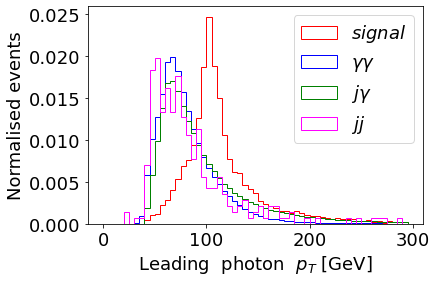
(a)

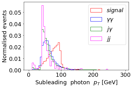
(b)

Figure 1: Left panel : Leading photon $p_{T}$ distribution of signal and backgrounds, Right panel: Sub-leading photon $p_{T}$ distribution of signal and backgrounds. Both distributions are shown for BP3

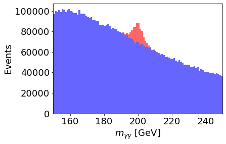
Figure 2: Invariant mass distribution (unnormalized, corresponding to $\int\mathcal{L}dt=3000fb\leavevmode\nobreak\ ^{-1}$) corresponding to BP3. The signal has been scaled up by a factor of 15. Events coming from background marked in blue and excess of events due to signal shown in red.

The distribution of leading and subleading photon $p_{T}$ for BP3 have been shown in Fig1 and the distribution in invariant mass of the diphoton system, corresponding to $\int\mathcal{L}dt=3000fb^{-1}$ is shown in Fig 2. From Fig 1, we can see that all the backgrounds lie mainly below, leading photon $p_{T}\approx 80\ GeV$ and subleading photon $p_{T}\approx 70\ GeV$ and the signal peaks at around 100 GeV leading and 90 GeV subleading photon $p_{T}$. In Fig 2, it is clear that the excess due to signal process, is prominent in the range of $195-205\ GeV$. Still we have retained $m_{\gamma\gamma}$ in the range i.e $170-230\ GeV$ in our analysis, since the procedure we adopted to calculate significance, relies on the measurement of background events in the sideband. These considerations have gone into the choice of cuts applied, which along with the cut-flow table are adumbrated in Table-2.

$m_{H}$[GeV]	cuts applied	signal [fb]	$\gamma\gamma$ [pb]	$j\gamma$ [pb]	jj [pb]
200	initial cross section	4.95	9.17	$4.89\times 10^{3}$	$2.01\times 10^{7}$
	acceptance	3.17	6.08	3.97	2.87
	$p_{T}^{l}\geq 70\ GeV\ ,\ p_{T}^{sl}\geq 60\ GeV$	2.72	2.02	1.35	0.64
	$170\ GeV\leq m_{\gamma\gamma}\leq 230\ GeV$	2.72	0.79	0.46	0.08

Table 2: The cut flow table corresponding to BP3. $p_{T}^{l}(p_{T}^{sl})$ corresponds to the leading (subleading) photon $p_{T}$.

5 Results of a cut-based analysis

5.1 Significance from likelihood ratio method

We have used, mutatis mutandis, the profile likelihood ratio method for binned data as formulated in reference [64] to calculate signal significance. We have used the distribution in $m_{\gamma\gamma}$ for this purpose.

The number of events in each bin is assumed to be a Poisson distribution. We start by modeling the signal with a Gaussian centered at $m_{H}$. Hence mean signal yield $s_{i}$ at $i^{th}$ bin is expressed as,

$$s_{i}=a_{1}e^{-\frac{(x_{i}-m_{H})^{2}}{2\sigma^{2}}}$$ (5.1)

$a_{1}$ and $\sigma$ were determined from the $m_{\gamma\gamma}$ distribution corresponding to signal, by maximizing likelihood. As found from the fit, $3\sigma\approx 10\leavevmode\nobreak\ GeV$ for BP2-BP5, while for BP1 $3\sigma\approx 5\leavevmode\nobreak\ GeV$. Hence for BP1, $(m_{H}\pm 5)\leavevmode\nobreak\ GeV$ and for the rest, $(m_{H}\pm 10)\leavevmode\nobreak\ GeV$ is defined as the signal region. The mean entry from background was estimated by blinding the signal region and fitting the sideband with an exponential function. Hence, expected event rate $\lambda_{b_{i}}$ in $i^{th}$ bin from background is given by,

$$\lambda_{b_{i}}=a_{0}e^{-bx_{i}}$$ (5.2)

where, $x_{i}$ is the bin center. Each type of background was modeled separately in the same way and the shape parameter $b$ was extracted from the fit while $a_{0}$ was determined using the number of events expected at $3000\leavevmode\nobreak\ fb^{-1}$.

With these, the expected number of events, $\lambda_{i}$ in $i^{th}$ bin is given by,

$$\lambda_{i}=a_{0}e^{-bx_{i}}+\mu a_{1}e^{-\frac{(x_{i}-m_{H})^{2}}{2\sigma^{2}}}$$ (5.3)

$a_{1}$ and $\sigma$ have been estimated from the signal. Except the signal parameters i.e $m_{H},a_{1}$ and $\sigma$, all other parameters $(a_{0},b,\mu)$ were allowed to vary freely in the fit. $\mu$ is the parameter of interest and $(a_{0},b)$ are the nuisance parameters. The normalizations a0 and a1 contain the cross section, Integrated luminosity, efficiency for background and signal respectively.

The likelihood function for the parameters $(a_{0},b,\mu)$,

$$\mathcal{L}_{(}a_{0},b,\mu)=\Pi_{i}\frac{\lambda_{i}^{n_{i}}e^{-\lambda_{i}}}{n_{i}!}$$ (5.4)

Where, $n_{i}$ is the observed number of events in the $i^{th}$ bin and the product is over the bins. The likelihood function for the parameters under background only hypothesis is given by,

$$\mathcal{L}_{1}(a_{0},b,\mu=0)=\Pi_{i}\frac{{\lambda_{b_{i}}}^{n_{i}}e^{-\lambda_{b_{i}}}}{n_{i}!}$$ (5.5)

$a_{0}$ and $b$ are evaluated by minimizing $-log(\mathcal{L}_{1})$. Finally the test statistic is given by,

$$q_{0} = -2log\frac{\mathcal{L}_{1}(\hat{\hat{a_{0}}},\hat{\hat{b}},\mu=0)}{\mathcal{L}_{2}(\hat{a_{0}},\hat{b},\hat{\mu})}\ \ \ \ \hat{\mu}\geq 0$$ (5.6)

$$= 0\ \ \ \ \hat{\mu}<0$$

In the denominator, ${\mathcal{L}_{2}(\hat{a_{0}},\hat{b},\hat{\mu})}$ denotes the global maximum of the likelihood function and $(\hat{a_{0}},\hat{b},\hat{\mu})$ are the values of $a_{0},\ b$ and $\mu$ that maximize the likelihood globally. In the numerator, ${\mathcal{L}_{1}(\hat{\hat{a_{0}}},\hat{\hat{b}}},\mu=0)$ denotes the maximum of the likelihood function for $\mu=0$, and $\hat{\hat{a_{0}}},\hat{\hat{b}}$ are the values of $a_{0},\ b$ that maximize the likelihood function when $\mu=0$. The significance is given by,

$$Z=\sqrt{q_{0}}$$ (5.7)

As shown in [64] in the asymptotic limit and when signal $(s)$ is much smaller than background $(B)$, Z becomes,

$$Z=\Sigma_{i}\frac{s_{i}}{\sqrt{B_{i}}}$$ (5.8)

where the sum is over the number of bins in the histogram. This explains the improvement in significance with a $\frac{s}{B}\approx 2\%$, even in presence of systematics.

To account for systematics, we generated toy Monte-Carlo samples for each background following the fit function given by,

$$\lambda_{b_{i}}=(1+\Delta_{s})a_{0}e^{-bx_{i}}$$ (5.9)

where $\Delta_{s}$ is the amount of systematic error. These backgrounds have been used to calculate significance in presence of systematics, by following the above mentioned procedure.

5.2 Parameter space with $\geq 3\sigma$ significance at $3000$ $fb^{-1}$

Finally we present the regions of the parameter space of the GM scenario, where the diphoton signal is discernible at the level of $3\sigma$ or more for an integrated luminosity of $3000\leavevmode\nobreak\ fb^{-1}$ at the LHC. The calculation of statistical significance has been carried out following the algorithm outlined in the previous subsection.

	$cut1$	$cut2$	significance	significance
			without systematics	with 10% systematics
BP1	$p_{T}^{l}>55,p_{T}^{sl}>45$	$130<m_{\gamma\gamma}<180$	10	9.4
BP2	$p_{T}^{l}>65,p_{T}^{sl}>55$	$150<m_{\gamma\gamma}<210$	5.7	5.3
BP3	$p_{T}^{l}>70,p_{T}^{sl}>60$	$170<m_{\gamma\gamma}<230$	7.6	7.1
BP4	$p_{T}^{l}>80,p_{T}^{sl}>70$	$190<m_{\gamma\gamma}<250$	10.4	10
BP5	$p_{T}^{l}>90,p_{T}^{sl}>80$	$210<m_{\gamma\gamma}<270$	9.1	8.7

Table 3: Analysis level cuts for each BP and corresponding significance both without systematics and with 10% systematics. $p_{T}^{l}(p_{T}^{sl})$ corresponds to the leading (subleading) photon $p_{T}$

Table 3 shows the significance corresponding to each BP, both with systematic uncertainty set to zero and with 10% systematic uncertainty. In order to obtain Fig 3 and Fig 6, the parameter space has been sliced into five parts corresponding to each BP with $m_{H}$ within the upper 20 GeV band of the benchmark $m_{H}$. The background as estimated for the BP has been used to calculate significance for the respective region. The signal cross-section has been obtained using Madgraph@MCNLO for each point in the parameter space and the efficiency factor of the BP has been multiplied to account for the cut efficiency.

We make some general observations below, based on Figure 3(a) - 3(e) where systematic errors has been set to zero, and the significance is given by equation (5.6) We shall comment later on the effect of including systematic errors, as shown in Figure 4.

(a)

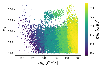
(b)

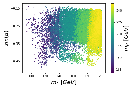
(c)

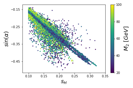
(d)

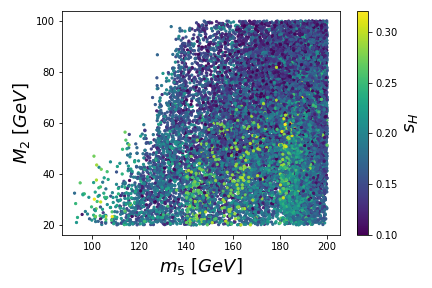
(e)

Figure 3: Regions of the parameter space that can be probed with a significance $\geq$ 3$\sigma$ at the HL-LHC, with $\int{\mathcal{L}}dt$ = 3000 $fb^{-1}$ without including any systematics.

• The predicted diphoton signals are expected to be significant in the region with $m_{H}$ approximately in the range 160 - 250 $GeV$, as seen from Figure 3(a).

• The same Figure also shows that the signal is favoured mostly for $m_{5}\leq m_{3}$. Even in the limited number of cases where the order is reversed, the splitting is mostly within 10-30 $GeV$. This serves to suppress the decay $H\rightarrow H^{+}_{3}W^{-}$, thus enhancing the diphoton decay branching ratio.

• As is also seen in Figure 3(b), $m_{5}\leq 200$ GeV favours the signal. This is also because the loop contributions are enhanced for low masses of the doubly charged scalar. $H^{+}_{3}$ also contributes significantly whenever the corresponding trilinear coupling is substantial.

• A substantial part of the the low $m_{5}$ region, yielding an appreciable signal strength, also corresponds to a relatively large $s_{H}$ (read the triplet contribution to the W/Z mass). This happens even when $H_{5}^{\pm\pm}$ decays exclusively to $W^{\pm}W^{\pm}$. The enhancement in $s_{H}$ happens due to the fact that the low mass $H_{5}^{\pm\pm}$ has a suppressed branching ratio to $W^{\pm}W^{\pm}$ and therefore the LHC bounds are more relaxed. Low $m_{H}$ too favours this, where the enhanced production rates due to large $s_{H}$ and hence large $k_{F}$ leads to fermionic signals which are liable to be swamped by backgrounds.

• Our favoured regions, indicated in the Figures, correspond to $Y_{ll}$, the $\Delta L=2$ Yukawa couplings being $\leq 10^{-6}$. For bigger $Y_{ll}$, the absence of same-sign dilepton signal puts stringent lower limits on $m_{5}$ [10], which causes suppression of the loop amplitudes leading to the diphoton signal.

• As all the panels in Fig 3 indicate, the signal is favoured for relatively low $m_{5}$ which is still allowed by all LHC-based studies reported so far. In this sense, the diphoton signals predicted by us can prove important in probing the low-$m_{5}$ regions in the GM parameter space, especially for $m_{5}\leq 200$ GeV, where the searches based on $H_{5}^{\pm\pm}$ production does not work so well. This is true even for diphotons seen with $\int\mathcal{L}dt=300\leavevmode\nobreak\ fb^{-1}$.

• Figures (3(c)-3(d)) show the signal regions in terms of $\sin\alpha$ as defined by equation (2.16), which is a measure of the doublet content of $H$, a features that decides its production rate in the gluon fusion channel. We find that the diphoton signal undergoes enhancement for large $|\sin\alpha|$, precisely due to the reason mentioned above.

• It is also seen from Figure 3(c) that for small $m_{H}$, a wide range of $m_{5}$ allows the signal to be substantial, while this privilege is exclusive to parameter regions with large $m_{5}$ when $m_{H}$ is high.

• Figure 3(e) shows that one can expect substantial signal strength even for small $M_{2}$, when $s_{H}$ is on the high side. This is because a high $s_{H}$ corresponds to a high $|sin\alpha|$ as evident in fig 3(d) which enhances the doublet component in $H$ and consequently its production rate via gluon fusion.

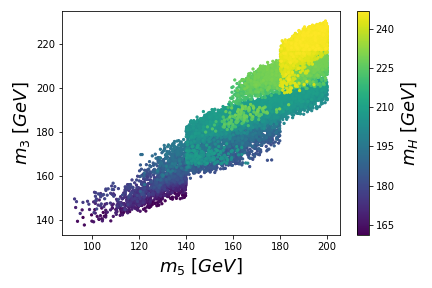
(a)

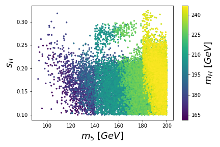
(b)

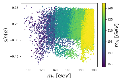
(a)

(b)

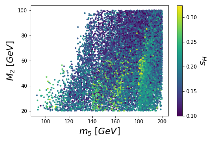
(a)

Figure 6: Regions of the parameter space that can be probed with a significance $\geq$ 3$\sigma$ at the HL-LHC, with $\int{\mathcal{L}}dt$ = 3000 $fb^{-1}$ in presence of 10% systematics.

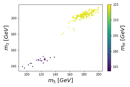
(a)

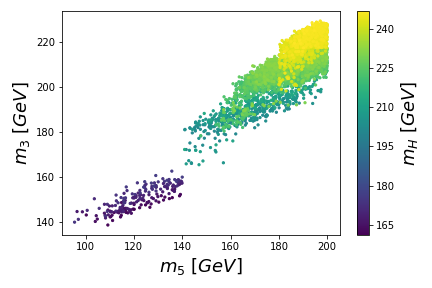
(b)

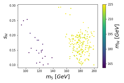
(c)

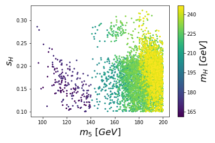
(d)

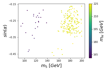
(e)

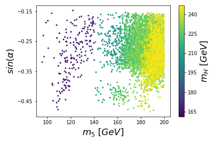
(f)

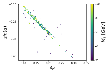
(g)

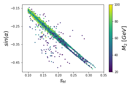
(h)

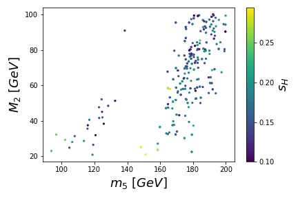
(i)

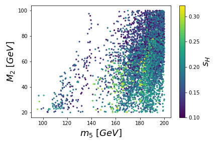
(j)

Figure 7: Left column: Same as in Fig 6 but with $\int{\mathcal{L}}dt$ = 300 $fb^{-1}$. Right column: Regions that can be probed at 2$\sigma$ level in presence of 10% systematics with $\int{\mathcal{L}}dt$ = 300 $fb^{-1}$.

We also show in Figure (4(a)-6(a)) the results of including 10% overall systematic error, following the prescription outlined in the previous subsection. A comparison between Figures 3 and 6 reveals that , no notable difference occurs due to the inclusion of this amount of sytematics.

Since the potential coverage of the GM parameter space via diphotons turns out rather optimistic, one might like to see how much can be achieved even before the HL-LHC begins its operation. With this in view, we also present in Fig 7 regions of parameter space which can be probed via diphotons with $\int{\mathcal{L}}dt$ = 300 $fb^{-1}$. This shows that the applicability of the diphoton signal become already noteworthy before Run-3 ends and certainly in the early phase of HL-LHC. For comparison, we also present in the same figure regions that can be probed at the 2$\sigma$ level with the same luminosity.

6 Summary and conclusions

We have identified the diphoton decay channel of the custodial SU(2) singlet scalar $H$ in the GM scenario as constituting a viable signal at the LHC. The main reasons for this enhancement are (a) contributions of the doubly-and singly-charged scalar loops, (b) suppression of the destructively interfering fermion loops, (c) enhancement of the relevant trilinear scalar couplings in certain regions of the parameter space, and (d) suppression of the tree-level fermion and gauge boson pair decays due to the dominant $SU(2)_{L}$ triplet composition of $H$ as compared to $h$. The two-photon final state, with invariant mass peaking at $m_{H}$, thus constitutes an independent search channel for the GM model, whose importance in multichannel analyses hardly needs to be emphasized for a scenario with several free parameters.

The major backgrounds come from SM contributions to $\gamma\gamma,j\gamma$ and $jj$ production, all of which have been taken into account in our simulation. The parameter space for the GM model has been scanned over, ensuring consistency with data from the 125-GeV scalar, general constraints from extended scalar sector searches, as also theoretical limits and indirect and precision electroweak constraints.

The signal significance has been computed using the profile likelihood ratio method. It is found that the regions most amenable to detection at the LHC are those corresponding to $m_{H}$ in the approximate range 160-180 and 220-240 GeV. We have identified the regions in the parameter space, for which the diphoton signal may have at least $3\sigma$ significance, with integrated luminosity of 3000 $fb^{-1}$ as well as 300 $fb^{-1}$. These results show that the diphoton channel constitutes a valuable component of the search strategy, along with those centered around doubly charged scalar production, even before the HL-LHC becomes operational and rather significantly with higher luminosities.

7 Acknowledgement

The work of R.G is supported by a fellowship awarded by University Grants Commission, India. The authors acknowledge the support provided by the Kepler Computing facility, maintained by the Department of Physical Sciences, IISER Kolkata, for various computational needs. We also thank Debabrata Bhowmik, Suman Dasgupta, Shubham Dutta, Deep Ghosh, Jayita Lahiri, Jyotiska Panda, Sirshendu Samanta, Tousik Samui, Ritesh K Singh and Amir Subba for helpful discussions.

References

- [1] S. L. Glashow, Nucl. Phys. 22, (1961) 579-588
- [2] J. Goldstone, A. Salam and S. Weinberg, Phys. Rev. 127, 965-970 (1962)
- [3] A. Salam, Conf. Proc. C 680519, 367-377 (1968)
- [4] S. Weinberg, Phys. Rev. Lett. 19, 1264-1266 (1967)
- [5] S. L. Glashow and S. Weinberg, Phys. Rev. D 15, 1958 (1977)
- [6] E. A. Paschos, Phys. Rev. D 15, 1966 (1977)
- [7] G. C. Branco, P. M. Ferreira, L. Lavoura, M. N. Rebelo, M. Sher and J. P. Silva, Phys. Rept. 516, 1-102 (2012) [arXiv:1106.0034 [hep-ph]].
- [8] P. H. Gu, H. Zhang and S. Zhou, Phys. Rev. D 74, 076002 (2006) [arXiv:hep-ph/0606302 [hep-ph]].
- [9] E. Ma and U. Sarkar, Phys. Rev. Lett. 80, 5716-5719 (1998).
- [10] R. Primulando, J. Julio and P. Uttayarat, JHEP 08, 024 (2019) [arXiv:1903.02493 [hep-ph]].
- [11] R. Ghosh, B. Mukhopadhyaya and U. Sarkar, J. Phys. G 50, 075003 (2023) [arXiv:2205.05041 [hep-ph]].
- [12] H. Georgi and M. Machacek, Nucl. Phys. B 262 (1985), 463
- [13] M. S. Chanowitz and M. Golden, Phys. Lett. B 165 (1985), 105
- [14] J. F. Gunion, R. Vega and J. Wudka, Phys. Rev. D 43 (1991), 2322
- [15] R. Ghosh and B. Mukhopadhyaya, Phys. Rev. D 107, 035031 (2023) [arXiv:2212.11688 [hep-ph]].
- [16] N. Ghosh, S. Ghosh and I. Saha, Phys. Rev. D 101, 015029 (2020) [arXiv:1908.00396 [hep-ph]].
- [17] C. W. Chiang, S. Kanemura and K. Yagyu, Phys. Rev. D 93, 055002 (2016) [arXiv:1510.06297 [hep-ph]].
- [18] C. W. Chiang and K. Yagyu, JHEP 01, 026 (2013) [arXiv:1211.2658 [hep-ph]].
- [19] B. Mukhopadhyaya, Phys. Lett. B 252, 123-126 (1990)
- [20] R. Godbole, B. Mukhopadhyaya and M. Nowakowski, Phys. Lett. B 352, 388-393 (1995) [arXiv:hep-ph/9411324 [hep-ph]].
- [21] D. K. Ghosh, R. M. Godbole and B. Mukhopadhyaya, Phys. Rev. D 55, 3150-3155 (1997) [arXiv:hep-ph/9605407 [hep-ph]].
- [22] K. m. Cheung, R. J. N. Phillips and A. Pilaftsis, Phys. Rev. D 51, 4731-4737 (1995) [arXiv:hep-ph/9411333 [hep-ph]].
- [23] T. K. Chen, C. W. Chiang, C. T. Huang and B. Q. Lu, Phys. Rev. D 106, 055019 (2022) [arXiv:2205.02064 [hep-ph]].
- [24] G. Aad et al. [ATLAS and CMS], Phys. Rev. Lett. 114, 191803 (2015) [arXiv:1503.07589 [hep-ex]].
- [25] A. M. Sirunyan et al. [CMS], Phys. Lett. B 805, 135425 (2020) [arXiv:2002.06398 [hep-ex]].
- [26] A. M. Sirunyan et al. [CMS], JHEP 07, 027 (2021) [arXiv:2103.06956 [hep-ex]].
- [27] K. Hartling, K. Kumar and H. E. Logan, Phys. Rev. D 91, 015013 (2015) [arXiv:1410.5538 [hep-ph]]
- [28] G. Aad et al. [ATLAS], JHEP 06, 146 (2021) [arXiv:2101.11961 [hep-ex]]
- [29] G. Aad et al. [ATLAS], Phys. Lett. B 822, 136651 (2021) [arXiv:2102.13405 [hep-ex]]
- [30] H. Bahl, T. Biekötter, S. Heinemeyer, C. Li, S. Paasch, G. Weiglein and J. Wittbrodt, Comput. Phys. Commun. 291, 108803 (2023) [arXiv:2210.09332 [hep-ph]]
- [31] M. Aaboud et al. [ATLAS], Eur. Phys. J. C 79, 58 (2019) [arXiv:1808.01899 [hep-ex]].
- [32] A. Ismail, H. E. Logan and Y. Wu, [arXiv:2003.02272 [hep-ph]].
- [33] Z. Bairi and A. Ahriche, Phys. Rev. D 108, 5 (2023) [arXiv:2207.00142 [hep-ph]].
- [34] T. K. Chen, C. W. Chiang, S. Heinemeyer and G. Weiglein, Phys. Rev. D 109, 075043 (2024) [arXiv:2312.13239 [hep-ph]]
- [35] A. Ahriche, [arXiv:2312.10484 [hep-ph]]
- [36] J. F. Gunion, R. Vega, and J. Wudka Phys. Rev. D 42 (1990), 1673
- [37] C. H. de Lima and H. E. Logan, Phys. Rev. D 106 (2022) [arXiv:2209.08393 [hep-ph]]
- [38] K. Hartling, K. Kumar and H. E. Logan, Phys. Rev. D 90, 015007 (2014) [arXiv:1404.2640v3 [hep-ph]]
- [39] M. E. Peskin and T. Takeuchi, Phys. Rev. Lett. 65, 964-967 (1990)
- [40] M. E. Peskin and T. Takeuchi, Phys. Rev. D 46, 381-409 (1992)
- [41] C. Degrande, K. Hartling and H. E. Logan, Phys. Rev. D 96, (2017) [erratum: Phys. Rev. D 98, (2018)] [arXiv:1708.08753 [hep-ph]]
- [42] P. Bechtle, O. Brein, S. Heinemeyer, G. Weiglein and K. E. Williams, Comput. Phys. Commun. 181, 138-167 (2010) [arXiv:0811.4169 [hep-ph]].
- [43] P. Bechtle, O. Brein, S. Heinemeyer, G. Weiglein and K. E. Williams, Comput. Phys. Commun. 182, 2605-2631 (2011) [arXiv:1102.1898 [hep-ph]].
- [44] P. Bechtle, O. Brein, S. Heinemeyer, O. Stal, T. Stefaniak, G. Weiglein and K. Williams, [arXiv:1301.2345 [hep-ph]].
- [45] P. Bechtle, O. Brein, S. Heinemeyer, O. Stål, T. Stefaniak, G. Weiglein and K. E. Williams, Eur. Phys. J. C 74, 2693 (2014) [arXiv:1311.0055 [hep-ph]].
- [46] P. Bechtle, S. Heinemeyer, O. Stal, T. Stefaniak and G. Weiglein, Eur. Phys. J. C 75, 421 (2015) [arXiv:1507.06706 [hep-ph]].
- [47] P. Bechtle, S. Heinemeyer, O. Stål, T. Stefaniak and G. Weiglein, Eur. Phys. J. C 74, 2711 (2014) [arXiv:1305.1933 [hep-ph]].
- [48] P. Bechtle, S. Heinemeyer, O. Stål, T. Stefaniak and G. Weiglein, JHEP 11, 039 (2014) [arXiv:1403.1582 [hep-ph]].
- [49] M. Aaboud et al. [ATLAS], JHEP 09, 139 (2018) [arXiv:1807.07915 [hep-ex]]
- [50] A. Tumasyan et al. [CMS], JHEP 07, 073 (2023) [arXiv:2208.02717 [hep-ex]]
- [51] HEPData
- [52] G. Aad et al. [ATLAS], Phys. Lett. B 822, 136651 (2021) [arXiv:2102.13405 [hep-ex]].
- [53] G. Aad et al. [ATLAS] Phys. Rev. D 85, 2012
- [54] S. Chatrchyan et al. [CMS], Eur. Phys. J. C 72, 2189 (2012) [arXiv:1207.2666 [hep-ex]]
- [55] S. P. Jones, M. Kerner and G. Luisoni, Phys. Rev. Lett. 120, 162001 (2018) [erratum: Phys. Rev. Lett. 128, 059901 (2022)] [arXiv:1802.00349 [hep-ph]].
- [56] J. Alwall, R. Frederix, S. Frixione, V. Hirschi, F. Maltoni, O. Mattelaer, H. S. Shao, T. Stelzer, P. Torrielli and M. Zaro, JHEP 07, 079 (2014) [arXiv:1405.0301 [hep-ph]]
- [57] A. Alloul, N. D. Christensen, C. Degrande, C. Duhr and B. Fuks, Comput. Phys. Commun. 185, 2250-2300 (2014) [arXiv:1310.1921 [hep-ph]].
- [58] R. Frederix, S. Frixione, V. Hirschi, D. Pagani, H. S. Shao and M. Zaro, JHEP 04, 076 (2017) [arXiv:1612.06548 [hep-ph]].
- [59] S. Carrazza, S. Forte and J. Rojo, [arXiv:1311.5887 [hep-ph]].
- [60] D. Bhowmik, J. Lahiri, S. Bhattacharya, B. Mukhopadhyaya and R. K. Singh, Eur. Phys. J. C 82, 914 (2022) [arXiv:2012.07822 [hep-ph]].
- [61] J. de Favereau et al. [DELPHES 3], JHEP 02, 057 (2014) [arXiv:1307.6346 [hep-ex]].
- [62] M. Cacciari, G. P. Salam and G. Soyez, JHEP 04, 063 (2008) [arXiv:0802.1189 [hep-ph]].
- [63] M. Cacciari, G. P. Salam and G. Soyez, Eur. Phys. J. C 72, 1896 (2012) [arXiv:1111.6097 [hep-ph]].
- [64] G. Cowan, K. Cranmer, E. Gross and O. Vitells, Eur. Phys. J. C 71, 1554 (2011) [erratum: Eur. Phys. J. C 73, 2501 (2013)] [arXiv:1007.1727 [physics.data-an]].