Quantum Dynamics with Stochastic Non-Hermitian Hamiltonians

Abstract

We study the quantum dynamics generated by a non-Hermitian Hamiltonian subject to stochastic perturbations in its anti-Hermitian part, describing fluctuating gains and losses. The master equation governing the noise-average dynamics describes a new form of dephasing. We characterize the resulting state evolution and analyze its purity. The novel properties of such dynamics are illustrated in a stochastic dissipative qubit. Our analytical results show that adding noise allows for a rich control of the dynamics, with a greater diversity of steady states and the possibility of state purification.

Quantum systems are always in contact with an environment. For this reason, any realistic description of quantum dynamics should include the effects of such coupling. The theory of open quantum systems (OQS) offers a wide range of approaches to this end Breuer and Petruccione (2007); Rivas and Huelga (2012). Two prominent approaches involve non-Hermitian (NH) Ashida et al. (2020); Plenio and Knight (1998); Moiseyev (2011) and stochastic Budini (2001); Chenu et al. (2017); Kiely (2021) Hamiltonians. NH Hamiltonians are generally associated with effective descriptions that account only for a subset of the total number of degrees of freedom of a quantum mechanical system. They can be obtained unraveling the Gorini-Kossakowski-Sudarshan-Lindblad (GKSL) equation Gorini et al. (1976); Lindblad (1976) and post-selecting the trajectories with no quantum jumps Ashida et al. (2020); Roccati et al. (2022), or using projector techniques, as often done in quantum optics, nuclear physics, and molecular quantum chemistry Plenio and Knight (1998); Moiseyev (2011); Feshbach (1958, 1962); Cohen‐Tannoudji et al. (1998). Recently, non-Hermitian Hamiltonians have regained interest because they display novel physical phenomena and topological phases Shen et al. (2018); Gong et al. (2018); Kawabata et al. (2018); Yao and Wang (2018); Takata and Notomi (2018); Yang et al. (2018); Guo et al. (2023) and provide understanding of the quantum Zeno effect Dubey et al. (2023); Snizhko et al. (2020).

NH Hamiltonians generally exhibit complex energy eigenvalues in which the imaginary part describes the lifetime of a state Gamow (1928); Cohen‐Tannoudji et al. (1998). Time evolution ceases then to be trace-preserving due to the leakage of probability density between the subspace under consideration and that associated with the remaining degrees of freedom. The evolution can be made trace-preserving (TP) by renormalizing the density matrix at all times, which renders the evolution nonlinear in the state Carmichael (2008); Brody and Graefe (2012); Alipour et al. (2020); Geller (2023); Rembieliński and Caban (2021). TP nonlinear dynamics has been realized experimentally by post-selection of any dissipative evolution, i.e., discarding the trajectories with quantum jumps Naghiloo et al. (2019); Chen et al. (2021). In this setting, the renormalization of the trace comes naturally as a restriction to the subset of trajectories with no quantum jumps. Furthermore, it allows us to study a plethora of dissipation-induced phenomena Abbasi et al. (2022); Erdamar et al. (2024); Harrington et al. (2022); Chen et al. (2022); Wang et al. (2023).

Stochastic Hamiltonians allow for a treatment of OQS in which the information of the environment is included through the noise statistics and the coupling to the noise Van Kampen (2011); Budini (2001); Kiely (2021). These appear naturally in the stochastic Schrödinger equations obtained by unraveling the GKSL equation in quantum trajectories Wiseman (1996); Wiseman and Milburn (2009); Carmichael (2008). Stochastic Hamiltonians can be used to engineer many-body and long-range interactions Chenu et al. (2017), and their behavior beyond the noise average relates to quantum information scrambling Martinez-Azcona et al. (2023).

Non-Hermitian Hamiltonians are typically studied in a deterministic setting. In this Letter, we go beyond this paradigm by studying the dynamics of NH Hamiltonians subject to classical noise, focusing on the effect of noise in the anti-Hermitian part of the Hamiltonian. Stochastic non-Hermitian Hamiltonians appear, e.g., in homodyne detection of the degenerate parametric oscillator Carmichael (1991). The stability of exceptional points under noise has also been investigated Wiersig (2020). Here, we consider the stochastic dynamics generated by a fluctuating non-Hermitian operator and derive an exact nonlinear master equation for the noise-averaged state dynamics, which recovers noise-induced quantum jumps. In general, this master equation is not of GKSL form and exhibits novel features. We derive an exact equation of motion for the purity and characterize the dynamics. Specifically, we identify the stable steady states in terms of the eigenvalues and eigenstates of the Liouvillian and show that they live in the subspace spanned by the eigenvectors whose eigenvalues’ real part is the largest. We illustrate these regimes by studying the dynamics in a stochastic dissipative qubit Naghiloo et al. (2019). Our analytical results provide the possible steady states, the spectral properties governing the dynamics, and the evolution of the purity.

Dynamics under anti-Hermitian fluctuations. We consider a system with Hermitian Hamiltonian $\hat{H}_{0}$ that is subject to classical noise coupled to the anti-Hermitian operators $i\hat{L}$, i.e.,

$$\hat{H}_{t}=\hat{H}_{0}-i(1+\sqrt{2\gamma}\xi_{t})\hat{L}.$$ (1)

This describes fluctuations around the mean in the Hermitian operator $\hat{L}=\hat{L}^{\dagger}$, with standard deviation $\sqrt{2\gamma}$. The classical noise is taken as Gaussian real white noise for simplicity, characterized by $\mathbb{E}(\xi_{t})=0$ and $\mathbb{E}(\xi_{t}\xi_{t^{\prime}})=\delta(t-t^{\prime})$, where $\mathbb{E}(\bullet)$ denotes the classical stochastic average. The (unnormalized) system density matrix for a single trajectory $\tilde{\varrho}_{t}$ evolves, over a small time increment, as $\tilde{\varrho}_{t+\mathrm{d}t}=\hat{U}_{\mathrm{d}t}\tilde{\varrho}_{t}\hat{U}^{\dagger}_{\mathrm{d}t}$, where the propagator $\hat{U}_{\mathrm{d}t}=\exp(-i\hat{H}_{0}\mathrm{d}t-\hat{L}\mathrm{d}t-\sqrt{2\gamma}\hat{L}\mathrm{d}W_{t})$ depends on the Wiener process $\mathrm{d}W_{t}=\xi_{t}\mathrm{d}t$. For Gaussian white noise, the latter obeys Itō’s rules Gardiner (1985): $\mathrm{d}W_{t}^{2}=\mathrm{d}t$ and $(\mathrm{d}W_{t})^{n}=0,\;\forall\;n>2$. Expanding the exponential dictating the evolution of the density matrix with these rules, we find a stochastic differential equation (SDE) for its evolution,

$$\mathrm{d}\tilde{\varrho}_{t}= \left(-i[\hat{H}_{0},\tilde{\varrho}_{t}]-\{\hat{L},\tilde{\varrho}_{t}\}+\gamma\{\hat{L},\{\hat{L},\tilde{\varrho}_{t}\}\}\right)\mathrm{d}t$$

$$-\sqrt{2\gamma}\{\hat{L},\tilde{\varrho}_{t}\}\mathrm{d}W_{t}.$$ (2)

We denote $\tilde{\rho}\equiv\mathbb{E}(\tilde{\varrho})$ the noise-averaged density matrix and use the tilde $\tilde{\bullet}$ to highlight that it is not normalized. Trace preservation can be imposed either by (i) renormalizing all single-trajectories and then average over the noise Carmichael (2008); Wiseman and Milburn (2009); Dubey et al. (2023); Benoist et al. (2021), or (ii) first averaging over the noise, and only then imposing trace preservation. These two approaches will generally yield different dynamics. We focus on the latter to capture the evolution of ensembles of trajectories and defer the former for future work.

The average over the noise of the unnormalized evolution reads

$$\frac{\mathrm{d}\tilde{\rho}_{t}}{\mathrm{d}t}=-i[\hat{H}_{0},\tilde{\rho}_{t}]-\{\hat{L},\tilde{\rho}_{t}\}+\gamma\{\hat{L},\{\hat{L},\tilde{\rho}_{t}\}\}\equiv\tilde{\mathcal{L}}[\tilde{\rho}_{t}]$$ (3)

for the noise-averaged density matrix, where $\tilde{\mathcal{L}}[\bullet]$ denotes the non-trace-preserving Liouvillian superoperator. This master equation can be formally solved as $\tilde{\rho}_{t}=e^{\tilde{\mathcal{L}}t}[\hat{\rho}_{0}]$. Imposing trace preservation at the average level yields the nonlinear master equation

$$\frac{\mathrm{d}\hat{\rho}_{t}}{\mathrm{d}t}= \;\tilde{\mathcal{L}}[\hat{\rho}_{t}]-\mathrm{Tr}(\tilde{\mathcal{L}}[\hat{\rho}_{t}])\hat{\rho}_{t},$$ (4)

$$= -i[\hat{H}_{0},\hat{\rho}_{t}]-\{\hat{L},\hat{\rho}_{t}\}+\gamma\{\hat{L},\{\hat{L},\hat{\rho}_{t}\}\}$$

$$+2\mathrm{Tr}(\hat{L}\hat{\rho}_{t})\hat{\rho}_{t}-4\gamma\mathrm{Tr}(\hat{L}^{2}\hat{\rho}_{t})\hat{\rho}_{t},$$

the solution of which is simply given by normalizing the non-trace-preserving (nTP) evolution, i.e., $\hat{\rho}_{t}\equiv\frac{\tilde{\rho}_{t}}{\mathrm{Tr}(\tilde{\rho}_{t})}=e^{\tilde{\mathcal{L}}t}[\hat{\rho}_{0}]/\mathrm{Tr}(e^{\tilde{\mathcal{L}}t}[\hat{\rho}_{0}]).$ Since the NH Hamiltonian is stochastic, the evolution leads to quantum jumps—terms of the form $\gamma\hat{L}\hat{\rho}_{t}\hat{L}$. Note that this master equation is not of the GKSL form; rather, it describes a new form of dephasing in which the jump operators act on the density matrix through a double anticommutator and do not conserve the norm of the state. A more general form is detailed in App. F. Similar equations, with a double anticommutator but with a minus sign, appear when studying the adjoint Liouvillian with fermionic jump operators and evolving operator Liu et al. (2023); Clark et al. (2010).

Note that, in general, the unnormalized evolution (3) can be trace-decreasing (TD), trace-preserving (TP), or trace-increasing (TI). While TD dynamics can easily be interpreted through post-selection, TI evolutions are conceptually challenging, even if sometimes deemed non-physical Nielsen and Chuang (2010) they can describe a biased ensemble of trajectories Garrahan and Lesanovsky (2010). Note that the present TI dynamics can always be made TD or TP by a gauge transformation in the master equation, namely, using an imaginary offset $-ia$ in (1) (cf. App. A).

We now characterize the dynamics generated by (4) in terms of the purity evolution and the stable steady states in the general setup before illustrating them in a stochastic dissipative qubit.

Purity dynamics. The purity $P_{t}=\mathrm{Tr}(\hat{\rho}_{t}^{2})$ evolves according to the differential equation

$$\partial_{t}P_{t}= -4\mathrm{Tr}(\hat{L}\hat{\rho}_{t}^{2})+4\gamma\left(\mathrm{Tr}(\hat{L}^{2}\hat{\rho}_{t}^{2})+\mathrm{Tr}(\hat{L}\hat{\rho}_{t}\hat{L}\hat{\rho}_{t})\right)$$

$$+4\mathrm{Tr}(\hat{L}\hat{\rho}_{t})P_{t}-8\gamma\mathrm{Tr}(\hat{L}^{2}\hat{\rho}_{t})P_{t}.$$ (5)

Evaluating this expression at $t=0$ yields the decoherence time $1/\tau_{P}\equiv\partial_{t}P_{t}|_{t=0}$. Whenever the state is pure, $\hat{\rho}_{t}=\ket{\Psi_{t}}\bra{\Psi_{t}}$, the terms coming from the deterministic anti-Hermitian part cancel out and the purity evolution $\partial_{t}P_{t}=-4\gamma{\rm Var}_{\Psi}(\hat{L})$ is dictated by the variance ${\rm Var}_{\Psi}(\hat{L})=\braket{\Psi_{t}}{\hat{L}^{2}}{\Psi_{t}}-\braket{\Psi_{t}}{\hat{L}}{\Psi_{t}}^{2}$. Thus, initial pure states exhibit a purity decay unless they are eigenstates of $\hat{L}$, in which case the purity remains constant at first order in $t$ ($\tau_{P}\rightarrow\infty$). This result is identical to the decoherence time of pure states in a dephasing channel and quantum Brownian motion Zurek (2003); Breuer and Petruccione (2007); Beau et al. (2017). Interestingly, this expression contains out-of-time-order terms reminiscent of OTOC’s Martinez-Azcona et al. (2023) and generalizes the known evolution for NH Hamiltonians Brody and Graefe (2012).

Long time dynamics: Stable steady states. To characterize the long-time dynamics, we use the right and left eigendecompositions of the non-trace-preserving Liouvillian superoperator, $\tilde{\mathcal{L}}[\tilde{\rho}_{\nu}]=\lambda_{\nu}\tilde{\rho}_{\nu}$ and $\tilde{\mathcal{L}}^{\dagger}[\tilde{\rho}_{\nu}^{\textsc{(l)}}]=\lambda_{\nu}^{*}\tilde{\rho}_{\nu}^{\textsc{(l)}}$, respectively. We define the eigenoperator basis as $\hat{\sigma}_{\nu}=\hat{\rho}_{\nu}/\mathrm{Tr}(\hat{\rho}_{\nu})$ if the operator has non-zero trace and as $\hat{\sigma}_{\nu}=\hat{\rho}_{\nu}$ if the operator is traceless. Furthermore, the eigenstate is physical when it is trace one, $\mathrm{Tr}(\sigma_{\nu})=1$, and positive semidefinite $\hat{\sigma}_{\nu}\geq 0$. The basis is ordered such that the physical states appear first $\nu<N_{\textsc{p}}$, the traceful states appear second $\nu<N_{\textsc{t}}$, and the traceless states come last. In each of the subsets, the states are further ordered by decreasing $\mathrm{Re}(\lambda_{\nu})$. Assuming the Liouvillian $\tilde{\mathcal{L}}$ to be diagonalizable, the evolution of the density matrix in this operator basis follows as

$$\!\!\!\hat{\rho}_{t} =\frac{\sum_{\nu=0}^{N^{2}-1}c_{\nu}e^{\lambda_{\nu}t}\hat{\sigma}_{\nu}}{\sum_{\mu=0}^{N_{\textsc{t}}-1}c_{\mu}e^{\lambda_{\mu}t}}\stackrel{{\scriptstyle t\rightarrow\infty}}{{\sim}}\hat{\sigma}_{0}{+}e^{-\Delta t}\sum_{\nu\in\mathbb{M}_{2}}\frac{c_{\nu}e^{i\omega_{\nu}t}}{c_{0}}\hat{\sigma}_{\nu},$$ (6)

where the coefficients are $c_{\nu}=\mathrm{Tr}(\hat{\sigma}_{\nu}^{\textsc{(l)}}\hat{\rho}_{0})/{\rm Tr}(\hat{\sigma}_{\nu}^{\textsc{(l)}}\hat{\sigma}_{\nu})$. All the physical states ($\hat{\sigma}_{\nu}$ with $\nu<N_{\textsc{p}}$) are steady states. However, only those whose eigenvalues have the largest real part $\hat{\sigma}_{0}$ are stable under all perturbations .

At long times, the stable steady state $\hat{\sigma}_{0}$ is the eigenvector associated with the eigenvalue with the largest real part over which there is an initial support, i.e., $\mathrm{Re}(\lambda_{0})=\max_{\nu}\mathrm{Re}(\lambda_{\nu})$ such that $c_{0}\neq 0$. The corrections to this state are suppressed at a rate dictated by the dissipative gap $\Delta=\mathrm{Re}(\lambda_{0}-\lambda_{1})$. They can oscillate with a frequency $\omega_{\nu}=\mathrm{Im}(\lambda_{\nu})$, depending on the presence or absence of complex eigenvalues in the set of states with the second largest real part, denoted by $\mathbb{M}_{2}$.

The long-time limit above assumes that the largest eigenvalue is real and non-degenerate. In a more general case, denoting $\mathbb{M}_{1}$ the set of states with the largest real part among those on which the initial state has nonzero support, the steady state follows as $\hat{\rho}^{\textsc{s}}=\frac{\sum_{\nu\in\mathbb{M}_{1}}^{N^{2}-1}c_{\nu}e^{i\omega_{\nu}t}\hat{\sigma}_{\nu}}{\sum_{\mu\in\mathbb{M}_{1}}^{N_{\textsc{t}}-1}c_{\mu}e^{i\omega_{\mu}t}}$.

Illustration: The stochastic dissipative qubit. Many of the exciting phenomena displayed by non-Hermitian Hamiltonians can be experimentally observed in a dissipative qubit Naghiloo et al. (2019); Chen et al. (2021); Abbasi et al. (2022); Erdamar et al. (2024); Harrington et al. (2022); Chen et al. (2022); Wang et al. (2023). The setting corresponds to the Lindblad evolution of a 3-level system $\{\ket{g},\ket{e},\ket{f}\}$, where all quantum jumps to $\ket{g}$ are discarded. This post-selection process leads to the effectively non-Hermitian Hamiltonian $\hat{H}=J\hat{\sigma}_{x}-i\Gamma\hat{\Pi}$, where $J$ is the hopping between $\ket{e}$ and $\ket{f}$, $\Gamma$ is the loss rate from $\ket{e}$ to $\ket{g}$ and $\hat{\Pi}=\ket{e}\bra{e}$ denotes the projector over state $\ket{e}$. The (shifted) spectrum $\varepsilon_{\pm}+i\frac{\Gamma}{2}=\pm\sqrt{J^{2}-\frac{\Gamma^{2}}{4}}$ is real for $J\geq\frac{\Gamma}{2}$, and imaginary for $J<\frac{\Gamma}{2}$. These two regimes respectively correspond to (passive) $\mathcal{PT}$ unbroken and broken symmetry phases Bender and Boettcher (1998).

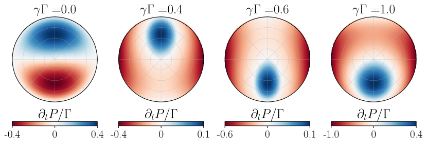
Figure 1: Purity evolution for different strengths of the noise as given by (9) in a cross-section of the Bloch sphere.

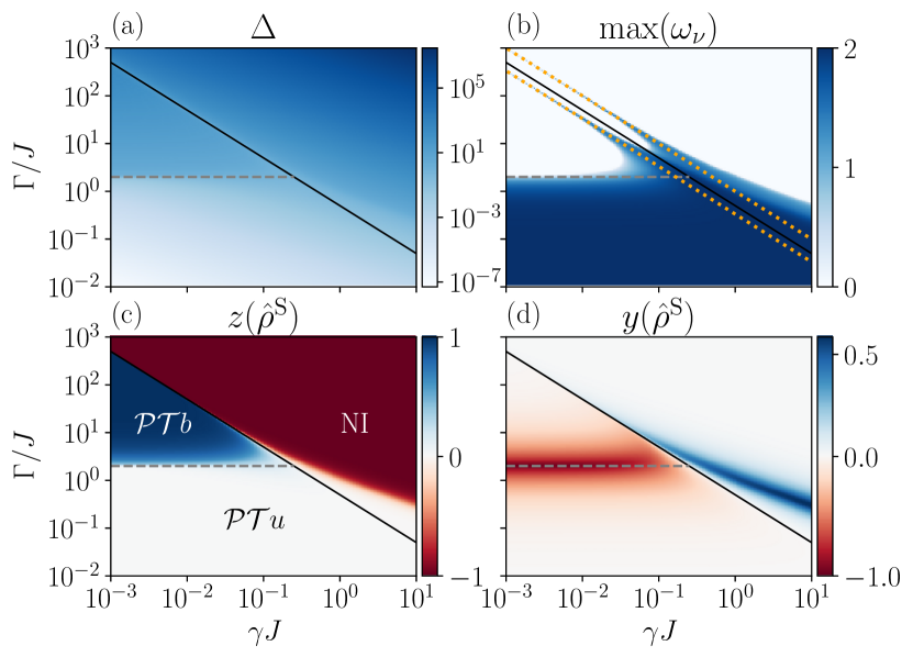
Figure 2: Spectral and steady-state phase diagrams: (a) dissipative gap $\Delta$, (b) maximum imaginary part of the eigenvalues $\omega_{\nu}$, (c) $z$, and (d) $y$ components of the Bloch vector for the stable steady state. The relevant parameters are the strength of the noise $\gamma$ and the decay rate $\Gamma$. The transition to the noise-induced phase is at $\gamma^{*}=1/(2\Gamma)$ (black). The transition from $\mathcal{PT}$ broken to the $\mathcal{PT}$ unbroken phase happens at $\Gamma/J=2$ (gray dashed). In (b) the power laws $\gamma=1/(3\Gamma)$ and $\gamma=1/\Gamma$ are also shown (orange dotted).

In this work, we are interested in the effect of noise in the anti-Hermitian part of the Hamiltonian. We thus consider a Stochastic Dissipative Qubit (SDQ) with time-dependent Hamiltonian

$$\hat{H}^{\textsc{sdq}}_{t}=J\hat{\sigma}_{x}-i\Gamma(1+\sqrt{2\gamma}\xi_{t})\hat{\Pi},$$ (7)

which physically corresponds to considering Gaussian fluctuations in the decay parameter $\Gamma$, with strength $\gamma$. The master equation (4) for this system reads

$$\partial_{t}\hat{\rho}_{t} =-iJ[\hat{\sigma}_{x},\hat{\rho}_{t}]-(\Gamma-\gamma\Gamma^{2})\{\hat{\Pi},\hat{\rho}_{t}\}+2\gamma\Gamma^{2}\hat{\Pi}\hat{\rho}_{t}\hat{\Pi}$$

$$\quad+(2\Gamma-4\gamma\Gamma^{2})\mathrm{Tr}(\hat{\Pi}\hat{\rho}_{t})\hat{\rho}_{t}.$$ (8)

Note that the trace of the unnormalized Liouvillian acting on any state reads $\mathrm{Tr}(\tilde{\mathcal{L}}[\hat{\rho}])=(4\gamma\Gamma^{2}-2\Gamma)\mathrm{Tr}(\hat{\Pi}\hat{\rho})$. As $\mathrm{Tr}(\hat{\Pi}\hat{\rho})\geq 0$, the dynamics is trace-decreasing when $4\gamma\Gamma^{2}-2\Gamma<0$ and trace-increasing when $4\gamma\Gamma^{2}-2\Gamma>0$. Therefore, the dynamics exhibits a transition from TD to TI at $\gamma^{*}=\frac{1}{2\Gamma}$. At this critical value, the nonlinear term vanishes: the dynamics is Completely Positive and Trace Preserving (CPTP), and its generator admits the standard GKSL form, with jump operator $\hat{\Pi}$ and rate $\Gamma$. When the Hamiltonian is Hermitian ($\Gamma=0$), the dynamics is trivially unitary. The noise can be used to tune the success rate, i.e. the number of trajectories with no jumps. For TD dynamics, this success rate corresponds to the trace $\mathrm{Tr}(\tilde{\rho}_{t})\propto\exp((4\gamma\Gamma^{2}-2\Gamma)t)$. If the noise increases this decay is slower, thus, a stronger noise $\gamma$ can be used to mitigate the decay of the success rate, especially near the critical value $\gamma^{*}$.

Every state of a qubit can be expressed in the Bloch sphere as $\hat{\rho}_{t}=\frac{1}{2}(\mathbb{1}+\mathbf{r}_{t}\cdot\hat{\boldsymbol{\sigma}})$ Nielsen and Chuang (2010). Expressing the Bloch vector $\mathbf{r}_{t}=(x_{t},y_{t},z_{t})$ in spherical coordinates $(r_{t},\theta_{t},\phi_{t})$, the purity (5) evolves for any state $\hat{\rho}_{t}$ as

$$\!\!\!\partial_{t}P_{t}=\Gamma r_{t}\left[(2\gamma\Gamma-1)(r_{t}^{2}-1)\cos\theta_{t}-\gamma\Gamma r_{t}\sin^{2}\theta_{t}\right].$$ (9)

Note that this expression shows a change in behavior at the TD-TI transition $\Gamma\gamma=\frac{1}{2}$. When $\Gamma\gamma<\frac{1}{2}$, the purifying states are in the north hemisphere of the Bloch ball, while for $\Gamma\gamma>\frac{1}{2}$, these states are shifted to the southern hemisphere, see Fig. 1.

We now investigate the spectral properties of the SDQ Liouvillian (8). The phase diagrams in Fig. 2 have three distinct phases: at weak noise $\gamma$, the notions of $\mathcal{PT}$ broken $\Gamma/J>2$ and unbroken $\Gamma/J<2$ symmetry of the NH Hamiltonian govern the dynamics, while at large noise strength, we see a transition to the TI dynamics at $\gamma^{*}$. We refer to these phases as $\mathcal{PT}$ broken ($\mathcal{PT}$b), $\mathcal{PT}$ unbroken ($\mathcal{PT}$u) and Noise Induced (NI). Figure 2(a) shows the dissipative gap $\Delta$ as a function of the noise strength $\gamma$ and the decay rate $\Gamma$. In the $\mathcal{PT}$u phase, the dissipative gap is very small, and thus the convergence to the stable steady state is very slow. In the $\mathcal{PT}$b phase the gap is larger, therefore the steady state is reached faster than in the $\mathcal{PT}$u phase. In the NI phase, the gap is very large, ensuring fast convergence to the stable steady state [cf. Eq. (6)]. Note that the gap is always smaller around the transition to the NI phase, which implies that the GKSL dynamics have slower convergence to the stable steady state. Fig. 2(b) shows the maximum imaginary part of the eigenvalues of the Lindbladian, which dictate the oscillatory behavior of the dynamics. Deep in the $\mathcal{PT}$b and NI phases, the imaginary part vanishes, implying that the dynamics is not oscillatory. However, it is nonzero in the $\mathcal{PT}$u phase. This fact, along with the very small dissipative gap, shows what features of the $\mathcal{PT}$u phase survive the application of classical noise.

We now characterize the non-degenerate stable steady state $\hat{\rho}^{\textsc{s}}$. Figure 2(c) shows the $z$ component of the Bloch vector of $\hat{\rho}^{\textsc{s}}$, which reads $z(\hat{\rho}^{\textsc{s}})=-\frac{\lambda_{0}(\lambda_{0}-A)}{4+\lambda_{0}(\lambda_{0}-A)}$ (cf. App. B), where $\lambda_{0}$ denotes the eigenvalue with the largest real part and the constant $A=\frac{\Gamma}{J}(\gamma\Gamma-1)$. In the $\mathcal{PT}$u phase, the $z$ component is small, and the steady state is close to the completely mixed state. Thus, when a very small noise is added to the $\mathcal{PT}$ symmetric NH Hamiltonian, the time evolution leads to a highly mixed state at very long times. In the $\mathcal{PT}$b phase, $z$ is close to unity—so the stable steady state is close to $\ket{f}$, as losses induced by $\Gamma$ remove all population in the $\ket{e}$ state. In the NI phase, the steady state is $\ket{e}$—the state that originally leaked to the ground state. This can be interpreted as a noise-induced transition to stability Horsthemke and Lafever (2006) of the originally unstable state, a feature shared by other noisy dynamics Martinez-Azcona et al. (2023). The $y$ Bloch coordinate phase diagram in Fig. 2(d) shows that the transition from the mixed state to the $\ket{f}$ ($\ket{e}$) state happens by acquiring a negative (positive) value of the $y$ coordinate in the Bloch sphere. The analytic expression for this quantity is $y(\hat{\rho}^{\textsc{s}})=\frac{2\lambda_{0}}{4+\lambda_{0}(\lambda_{0}-A)}$ (cf. App. B).

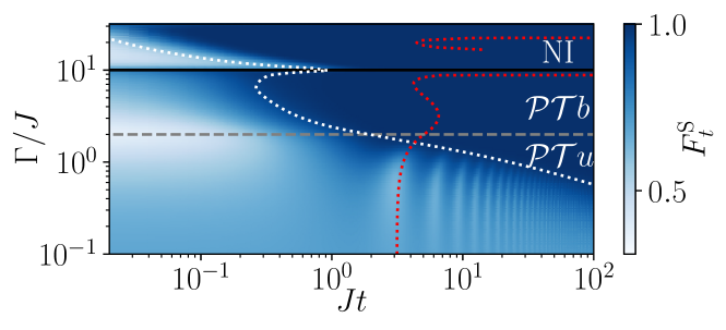
Figure 3: Fidelity between the time-evolved state and the stable steady state as a function of the loss parameter $\Gamma$ and time for noise strength $\gamma J=0.05$. $\mathcal{PT}$u to $\mathcal{PT}$b phase transition (gray dashed) and $\mathcal{PT}$b to NI phase transition (black). Time-scales of the dissipative gap $\Delta^{-1}$ (white dotted) and oscillatory dynamics $2\pi/\omega$ (red dotted).

Let us now turn to the dynamics generated by the master equation (8). The dynamics can be solved numerically in two complementary ways (cf. App. C, D). We characterize the distinguishability between the evolving and stable steady states using the Uhlmann fidelity $F^{\textsc{s}}_{t}=F(\hat{\rho}_{t},\hat{\rho}^{\textsc{s}})$ Uhlmann (1976); Bures (1969), which admits a compact form in a qubit system Jozsa (1994); Hübner (1992) (cf. App. E). Figure 3 shows the evolution of the fidelity as a function of time and the decay parameter $\Gamma$ for a small noise, $\gamma J=0.05$. This value ensures that the three different phases are manifested: (i) for $\Gamma/J<2$, the system is in the $\mathcal{PT}$u phase, and the fidelity to the steady state exhibits the anticipated oscillatory behavior until it vanishes at a time close to the inverse dissipative gap $t\sim\Delta^{-1}$ (white dotted line). The period of these oscillations is perfectly characterized by $2\pi/\omega$ where $\omega=\max_{\nu}\mathrm{Im}(\lambda_{\nu})$, as highlighted by the red dotted line. Note that this oscillatory frequency is affected by the increase of $\Gamma$ as we approach the $\mathcal{PT}$ phase transition, as also observed experimentally in the dissipative qubit Naghiloo et al. (2019). (ii) For $2<\Gamma/J<\frac{1}{2J\gamma}$, the system is in the $\mathcal{PT}$b phase, with a larger dissipative gap [cf. Fig. 2(a)], and thus a faster convergence to the steady state. Interestingly, the oscillatory timescale can be finite outside of the $\mathcal{PT}$u phase as $\omega$ does not vanish identically. In particular, it shows minima at $\Gamma=\frac{1}{3\gamma}$ and $\Gamma=\frac{1}{\gamma}$, as observed in Fig. 2(b). Exactly at the transition $\Gamma=\frac{1}{2\gamma}$, the dynamics is CPTP, and its convergence is slower, as explained by the smaller gap at the transition line. (iii) For $\Gamma>\frac{1}{2\gamma}$, the system is in the NI phase and exhibits the fastest convergence to the steady state. Experimentally, the decay rate is $\Gamma=6.7\;\mu\mathrm{s}^{-1}$ Naghiloo et al. (2019), which upper bounds the noise strength $\gamma<\gamma^{*}\approx 0.074\;\mu\mathrm{s}$ given that no NI phase was observed.

Conclusions. We have considered the time evolution governed by a fluctuating non-Hermitian Hamiltonian describing a quantum mechanical system subject to stochastic gain and loss. The resulting noise-averaged dynamics is described by a novel kind of master equation beyond the GKSL form. We characterized the purity dynamics and found that the stable steady states live in the Liouvillian eigenspace whose eigenvalues have the largest real part. The salient features of such dynamics are manifested in a stochastic dissipative qubit. The addition of noise allows for control over the steady states and the rate of convergence. We find three main dynamical phases: the $\mathcal{PT}$ unbroken and broken regimes, complemented with a noise-induced phase. Our results are amenable to current experimental platforms realizing non-Hermitian evolution. Our findings suggest that engineering fluctuating operators associated with gain and loss may open new avenues for quantum state preparation Verstraete et al. (2009). Our results may also be applied to understand the stability of imaginary time evolution Motta et al. (2020) against classical noise.

Acknowledgements— We thank Oskar Prosniak, Kohei Kawabata, and Martin Plenio for their insightful discussions and Shiue-Yuan Shiau for comments on the manuscript. This research was funded by the Luxembourg National Research Fund (FNR, Attract grant 17132054 and grant 17132054). The work at Los Alamos was supported by the U.S. Department of Energy.

Appendix A Gauge transformations of the nonlinear master equation

We discuss below how trace-increasing dynamics can be changed, such as to conserve or reduce the state trace. For this, we explicitly distinguish the stochastic $\hat{L}_{\textsc{s}}$ and deterministic $\hat{L}_{\textsc{d}}$ parts of the anti-Hermitian part of the Hamiltonian, and add an imaginary deterministic shift $a\in\mathbb{R}$. Namely, we consider

$$\hat{H}_{t}^{\prime}=\hat{H}_{0}-i(\hat{L}_{\textsc{d}}+a\,\hat{\mathbb{1}})-i\sqrt{2\gamma}\xi_{t}\hat{L}_{\textsc{s}},$$ (10)

which generates the nonlinear master equation

$$\partial_{t}\hat{\rho}_{t}= -i[\hat{H}_{0},\hat{\rho}_{t}]-\{\hat{L}_{\textsc{d}}+a\,\hat{\mathbb{1}},\hat{\rho}_{t}\}+\gamma\{\hat{L}_{\textsc{s}},\{\hat{L}_{\textsc{s}},\hat{\rho}_{t}\}\}$$

$$+2\mathrm{Tr}\big{(}(\hat{L}_{\textsc{d}}+a\,\hat{\mathbb{1}})\hat{\rho}_{t}\big{)}\hat{\rho}_{t}-4\gamma\mathrm{Tr}(\hat{L}_{\textsc{s}}^{2}\hat{\rho}_{t})\hat{\rho}_{t}.$$ (11)

Systems with any shift $a$ have the same dynamics, since the terms $-\{a\,\hat{\mathbb{1}},\hat{\rho}_{t}\}$ and $+2\mathrm{Tr}(a\hat{\rho}_{t})\hat{\rho}_{t}$ exactly cancel each other. This provides a non-Hermitian generalization of the well-known fact that shifting the Hamiltonian by a constant $\hat{H}+a\mathbb{1}$ has no consequence on the dynamics. Thus, a complex zero of energy also has no dynamical effect, provided that the trace of the density matrix is renormalized. It follows that the dynamics can be made TD or even TP with a suitable choice of $a$, namely

$$4\gamma\mathrm{Tr}(\hat{L}^{2}_{\textsc{s}}\hat{\rho}_{t})-2\mathrm{Tr}(\hat{L}_{\textsc{d}}\hat{\rho}_{t})-a\leq 0,$$ (12)

where ‘$<$’ corresponds to a TD map and ‘$=$’ to TP dynamics.

For the SDQ considered in the main text, $\hat{L}_{\textsc{d}}=\hat{L}_{\textsc{s}}=\Gamma\hat{\Pi}$, so the shift has to obey the condition

$$a\geq(4\gamma\Gamma^{2}-2\Gamma)\mathrm{Tr}(\hat{\Pi}\hat{\rho}),$$ (13)

for any $\hat{\rho}$. Since the expectation value has the property $\mathrm{Tr}(\hat{\Pi}\hat{\rho})=\rho_{ee}\leq 1$, a looser but state-independent condition on the shift reads

$$a\geq 4\gamma\Gamma^{2}-2\Gamma=BJ.$$ (14)

Alternatively, consider a gauge transformation that shifts the stochastic component by a constant $b\in\mathbb{R}$

$$\hat{H}_{t}^{\prime}=\hat{H}_{0}-i\hat{L}^{\prime}_{\textsc{d}}-i\sqrt{2\gamma}\xi_{t}(\hat{L}_{\textsc{s}}+b\hat{\mathbb{1}}),$$ (15)

which generates the nonlinear master equation

$$\partial_{t}\hat{\rho}_{t}= -i[\hat{H}_{0},\hat{\rho}_{t}]-\{\hat{L}^{\prime}_{\textsc{d}}-4\gamma b\hat{L}_{\textsc{s}},\hat{\rho}_{t}\}+\gamma\{\hat{L}_{\textsc{s}},\{\hat{L}_{\textsc{s}},\hat{\rho}_{t}\}\}$$

$$+2\mathrm{Tr}((\hat{L}^{\prime}_{\textsc{d}}-4\gamma b\hat{L}_{\textsc{s}})\hat{\rho}_{t})\hat{\rho}_{t}-4\gamma\mathrm{Tr}(\hat{L}^{2}_{\textsc{s}}\hat{\rho}_{t})\hat{\rho}_{t}.$$ (16)

It follows that the transformation

$$\begin{cases}\hat{L}_{\textsc{s}}\rightarrow\hat{L}_{\textsc{s}}+b\,\hat{\mathbb{1}},\\ \hat{L}_{\textsc{d}}\rightarrow\hat{L}_{\textsc{d}}+4\gamma b\,\hat{L}_{\textsc{s}},\end{cases}$$ (17)

also leaves the nonlinear master equation invariant. This transformation, similar to the GKSL case Breuer and Petruccione (2007), allows choosing jump operators $\hat{L}_{\textsc{s}}$ that are traceless.

Appendix B Liouvillian spectrum of the Stochastic Dissipative Qubit

The master equations given in the main text can be formulated in Liouville superspace. To this end, the density operator is written as a vector $|\tilde{\rho})$ of the form

$$\tilde{\rho}=\sum_{n,m}\tilde{\rho}_{nm}\ket{n}\bra{m}\;\mapsto\;|\tilde{\rho})=\sum_{n,m}\tilde{\rho}_{nm}\ket{n}\otimes\ket{m}^{*};$$ (18)

we refer the reader to Gyamfi (2020) for a detailed description of this procedure. Superoperators are mapped to operators on the superspace following the Choi-Jamiołkowski isomorphism Choi (1975); Jamiołkowski (1972)

$${\hat{X}}\tilde{\rho}{\hat{Y}}\;\mapsto\;({\hat{X}}\otimes{\hat{Y}}^{\intercal})|\tilde{\rho}),$$ (19)

where $\otimes$ denotes the Kronecker product and $\bullet^{\intercal}$ the transpose.

Vectorization requires fixing the inner product to be taken between operators; in the above procedure, the inner product is chosen as the standard Hilbert-Schmidt inner product $(X|Y)=\mathrm{Tr}(\hat{X}^{\dagger}\hat{Y})$, which for vectorized operators conveniently reduces to the standard euclidean inner product for vectors, $(X|Y)=\sum_{m,n}X_{mn}^{*}Y_{mn}$.

The non-trace-preserving state dynamics is then dictated by $\frac{\mathrm{d}}{\mathrm{d}t}|\tilde{\rho})=\tilde{\mathcal{L}}|\tilde{\rho})$ with the vectorized Liouvillian superoperator in (3) given by

$$\begin{split}\tilde{\mathcal{L}}=&-i(\hat{H}_{0}\otimes\hat{\mathbb{1}}-\hat{\mathbb{1}}\otimes\hat{H}_{0}^{\intercal})-(\hat{L}\otimes\hat{\mathbb{1}}+\hat{\mathbb{1}}\otimes\hat{L}^{\intercal})\\ &+\gamma(\hat{L}^{2}\otimes\hat{\mathbb{1}}+\hat{\mathbb{1}}\otimes(\hat{L}^{2})^{\intercal}+2\hat{L}\otimes\hat{L}^{\intercal}).\end{split}$$ (20)

Similarly, the Liouvillian for the SDQ (8) is given in matrix form by

$$\tilde{\mathcal{L}}=J\left(\begin{array}[]{cccc}0&i&-i&0\\ i&A&0&-i\\ -i&0&A&i\\ 0&-i&i&B\end{array}\right),$$ (21)

where we have defined the constants $A=\frac{\Gamma}{J}(\gamma\Gamma-1)$ and $B=2\frac{\Gamma}{J}(2\gamma\Gamma-1)$. The characteristic polynomial of the Liouvillian thus reads

$$(A-\Lambda)f(\Lambda)=0,$$ (22)

with the cubic polynomial $f(\Lambda)=\Lambda^{3}-\Lambda^{2}(A+B)+\Lambda(4+AB)-2B$. To find its roots, we first shift the variable, using $z=\Lambda-(A+B)/3$ and get a depressed cubic, i.e. a cubic equation without quadratic term

$$f(z)=z^{3}+3Cz+D=0,$$ (23)

with the constants $C=-\big{(}\frac{A+B}{3}\big{)}^{2}+\frac{4+AB}{3}$ and $D=\frac{A+B}{3}(4+AB)-2B-2\big{(}\frac{A+B}{3}\big{)}^{3}$. We then use Cardan’s trick Nickalls (1993), also known as Vieta’s substitution, that is, set $z=U+\frac{a}{U}$, choosing $a$ to remove the terms in $U$ and $1/U$, i.e., $a=-C$. This leads to a quadratic equation in $U^{3}$,

$$(U^{3})^{2}+DU^{3}-C^{3}=0,$$ (24)

with solutions $U_{m,\pm}=e^{mi\frac{2\pi}{3}}\big{[}-\frac{D}{2}\pm\sqrt{\big{(}\frac{D}{2}\big{)}^{2}+C^{3}}\big{]}^{1/3}$, with $m=(0,\pm 1)$. The Liouvillian eigenvalues follow as

$$\Lambda_{m,\pm}=J\left(U_{m,\pm}-\frac{C}{U_{m,\pm}}+\frac{A+B}{3}\right).$$ (25)

Note that we seem to have obtained 6 solutions from a cubic equation. However, three pairs of solutions are the same. To show this, let $V=-\frac{D}{2}\pm\sqrt{\frac{D^{2}}{4}+C^{3}}\equiv U_{m,\pm}^{3}$ denote any nonzero root of the quadratic equation (24). If $V$ is a root then $\frac{-C^{3}}{V}$ is also a root; this implies that if we change $+\rightarrow-$ in $\Lambda_{m,\pm}$ we exchange the terms $U_{m,\pm}$ with the term $-\frac{C}{U_{m,\pm}}$. So it is enough to consider the eigenvalues $\Lambda_{m,+}$.

We denote the eigenvalues $\{\lambda_{0}\equiv\Lambda_{0,+},\lambda_{1}\equiv\Lambda_{1,+},\lambda_{2}\equiv\Lambda_{-1,+},\lambda_{3}=AJ\}$ that diagonalize the Liouvillian (21),

$$\tilde{\mathcal{L}}=\sum_{\nu=0}^{3}\lambda_{\nu}|B_{\nu})(B_{\nu}|.$$ (26)

In the domain of interest, with $\gamma$ and $\Gamma$ positive, $\lambda_{0}$ is the eigenvalue with the maximum real part. This feature is verified for a wide range of parameters in Fig. 4, where the maximum difference of the real part of eigenvalues $\lambda_{\nu}$ for $\nu\geq 1$ and $\lambda_{0}$ is always shown to be negative. The full spectrum can be checked for many different parameters in Fig. 5. This plot allows us to see the large dissipative gap and no oscillatory behavior in the NI phase (a3, a4, b4), as well as the non-zero imaginary components and a small gap in the $\mathcal{PT}$u phase (c1-3), and the intermediate gap and no oscillations in the $\mathcal{PT}$b phase (a1), as well as the transitions between them

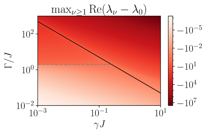
Figure 4: Maximum difference of the real part of $\lambda_{\nu},\nu\geq 1$ with $\lambda_{0}$. The difference is always negative for the displayed range of parameters, therefore $\lambda_{0}$ is always the eigenvalue with the largest real part. The transitions between the $\mathcal{PT}$u, $\mathcal{PT}$b, and NI phases are shown in the dashed and solid line as in Fig. 2 of the main text.

Figure 5: Spectrum of the SDQ Liouvillian for different locations in the phase diagram of the system. The parameters span the different phases: (a1) $\mathcal{PT}$ broken, (c1-3) $\mathcal{PT}$ unbroken, and (a3, a4, b4) Noise Induced; as well as the transitions between them: (b1,2) $\mathcal{PT}$ breaking transition, (a2,b3) TD-TI transition and (c4) transition from mixed state to $\ket{e}$ state. Note that the $x$-axis has been rescaled by $\Gamma/J$.

The eigenvector $|B_{0})=(b_{0}^{(0)},b_{1}^{(0)},b_{2}^{(0)},b_{3}^{(0)})^{\intercal}$ associated to the eigenvalue $\lambda_{0}$ is given by the solution of the system of equations

$$\begin{cases}+i(b^{(0)}_{1}-b^{(0)}_{2})=\lambda_{0}b^{(0)}_{0},\\ +i(b^{(0)}_{0}-b^{(0)}_{3})=(\lambda_{0}-A)b^{(0)}_{1},\\ -i(b^{(0)}_{0}-b^{(0)}_{3})=(\lambda_{0}-A)b^{(0)}_{2},\\ -i(b^{(0)}_{1}-b^{(0)}_{2})=(\lambda_{0}-B)b^{(0)}_{3}.\\ \end{cases}$$ (27)

By substitutions, given that $\lambda_{0}$ is the largest eigenvalue, in particular $\lambda_{0}>A$, we find

$$b^{(0)}_{3}=b^{(0)}_{0}\left(1+\lambda_{0}\frac{\lambda_{0}-A}{2}\right)$$ (28)

and $b^{(0)}_{1}=-b^{(0)}_{2}=-ib^{(0)}_{0}\lambda_{0}/2$. We choose $b^{(0)}_{0}$ such as to normalize the eigenvector for real $\lambda_{0}$, yielding the eigenvector associated to the stable steady state

$$|B_{0})=\frac{1}{2+\lambda_{0}\frac{\lambda_{0}-A}{2}}\left(\begin{array}[]{c}1\\ -\frac{i}{2}\lambda_{0}\\ \frac{i}{2}\lambda_{0}\\ 1+\lambda_{0}\frac{\lambda_{0}-A}{2}\end{array}\right).$$ (29)

Appendix C Bloch sphere dynamics for the Stochastic Dissipative Qubit

Any density matrix of a qubit $\hat{\rho}$ is completely characterized by its Bloch coordinates $\mathbf{r}=(x,y,z)$ from the decomposition

$$\hat{\rho}=\frac{1}{2}(\hat{\mathbb{1}}+\mathbf{r}\cdot\hat{\boldsymbol{\sigma}}),$$ (30)

where $\hat{\boldsymbol{\sigma}}$ is a vector containing the Pauli matrices obeying the standard commutation $[\hat{\sigma}_{n},\hat{\sigma}_{m}]=2i\epsilon_{nml}\hat{\sigma}_{l}$, and anticommutation $\{\hat{\sigma}_{n},\hat{\sigma}_{m}\}=2\delta_{nm}\hat{\mathbb{1}}$ relations.

For the SDQ, the master equation (4) in the main text dictates the evolution of these coordinates according to the coupled differential equations

$$\begin{cases}\dot{x}=-(\gamma\Gamma^{2}+z\Gamma(1-2\gamma\Gamma))x,\\ \dot{y}=-2Jz-(\gamma\Gamma^{2}+z\Gamma(1-2\gamma\Gamma))y,\\ \dot{z}=2Jy-\Gamma(1-2\gamma\Gamma)(z^{2}-1).\end{cases}$$ (31)

The streamlines of this vector field, as well as the analytical steady state $|B_{0})$ (29) are compared in Fig. 6. We see perfect agreement between the analytical steady state (red diamond) and the evolution of the streamlines showing convergence to it.

The behavior discussed in the main text is also apparent from these coordinates: (i) the $\mathcal{PT}$b phase has a steady state in the north pole, very close to the $\ket{f}$ state [cf. Fig. 6(a1)]; (ii) the $\mathcal{PT}$u phase [cf. Fig. 6(c1-3)] has a steady state close to the maximally mixed state in the center of the sphere, with a small $y$ component, as observed in Fig. 2(d) of the main text and (iii) the NI phase [cf. Fig. 6(a3-4, b4)] has a steady state very close to the $\ket{e}$ state in the south pole of the sphere.

The transition between the different phases also exhibits an interesting behavior: In the $\mathcal{PT}$u to $\mathcal{PT}$b phase transition (cf. Fig. 6 (b1-2)), we see a convergence to a state close to $\ket{-y}=\frac{\ket{f}-i\ket{e}}{\sqrt{2}}$, interestingly, the color scale shows that the speed of this convergence is larger the dissipative gap or the oscillatory timescale; the transition from TD to TI dynamics is also interesting (cf. Fig. 6 (a2, b3)), in this transition the dynamics is CPTP, and the steady state is the maximally mixed state in the center of the Bloch ball, to which the convergence shows almost no oscillations in (a2) and an oscillatory behavior in (b3), see Fig. 5 to understand this. Lastly, the transition from $\mathcal{PT}$u to the NI phases (cf. Fig. 6 (c4)) shows an oscillatory convergence to the steady state, which has a positive component of $y$, as already known from Fig. 2 (d).

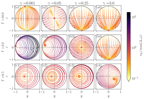
Figure 6: Streamlines of the vector fields in the cross-section of the Bloch sphere with $x=0$. The parameters span the different phases: (a1) $\mathcal{PT}$ broken, (c1-3)$\mathcal{PT}$ unbroken, and (a3, a4, b4) Noise Induced; as well as the transitions between them: (b1,2) $\mathcal{PT}$ breaking transition, (a2,b3) TD-TI transition and (c4) transition from mixed state to $\ket{e}$ state. The analytical steady state (29) is shown as the red diamond. The color and linewidth represent the Euclidean speed $v_{E}=\sqrt{(\dot{y})^{2}+(\dot{z})^{2}}$, divided by the maximum of the two main frequency units: the dissipative gap $\Delta$ and the maximum imaginary part of the eigenvalues $\omega=\max_{\nu}(\mathrm{Im}(\lambda_{\nu}))$.

Appendix D Comparison of different numerical approaches

We now compare two different numerical resolutions of the SDQ dynamics. The first is to numerically integrate the nonlinear system of differential equations (31)—we do so by a standard 4th-order Runge-Kutta (RK4) method. The second approach is to get the time evolution of the density matrix from the formal solution of the master equation, i.e. $|\tilde{\rho}_{t})=e^{\tilde{\mathcal{L}}t}|\rho_{0})$, where the equation is vectorized to compute the map $e^{\tilde{\mathcal{L}}t}[\bullet]$ simply through matrix exponentiation. Additionally, this method requires normalization of the state $|\rho_{t})=|\tilde{\rho}_{t})/\mathrm{Tr}(\tilde{\rho}_{t})$, where $\mathrm{Tr}(\tilde{\rho}_{t})=(\mathbb{1}|\tilde{\rho}_{t})=\tilde{\rho}_{ee}+\tilde{\rho}_{ff}$ and $\tilde{\rho}_{ee}=\bra{e}\tilde{\rho}_{t}\ket{e}$. To avoid computing a matrix exponential for each time $t$, we Trotterize the evolution as $e^{\tilde{\mathcal{L}}t}=\prod_{n=1}^{N_{\textsc{t}}}e^{\tilde{\mathcal{L}}\Delta_{\textsc{t}}}$, subdividing the evolution in $N_{\textsc{t}}$ steps of length $\Delta_{\textsc{t}}=t_{\rm end}/N_{\textsc{t}}$.

These two approaches are compared in Fig. 7 to compute the purity, showing a perfect agreement. Additionally, the first-order evolution of the purity obtained from $\partial_{t}P$ in (9) also agrees with the simulated evolution.

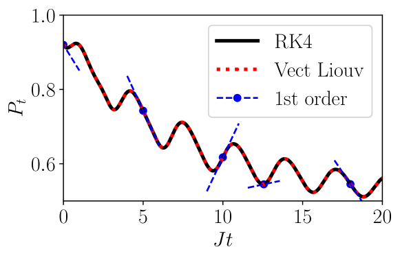
Figure 7: Purity computed from 4th-order Runge Kutta (black line) and using the vectorized Liouvillian (red dotted line). The first-order Taylor approximation, determined from the $\partial_{t}P$ formula (blue dashed line), matches the two approaches. The parameters for the simulation are $\gamma=0.5,\;\Gamma=0.5$ and the initial state has Bloch components $\mathbf{r}=(0.2,\;0.8,\;0.4)$. The absolute value of the difference between the two solutions is of order $10^{-11}$ with a timestep $J\Delta_{\textsc{t}}=0.004$.

Appendix E Uhlmann fidelity for a qubit

The fidelity between two pure states $\ket{\psi}$ and $\ket{\phi}$ measures how distinguishable the two states are, and is given by $F(\psi,\phi)=|\braket{\psi}{\phi}|^{2}=\mathrm{Tr}(\ket{\psi}\braket{\psi}{\phi}\bra{\phi})$ Nielsen and Chuang (2010). The generalization to any two mixed states $\hat{\rho},\;\hat{\sigma}$ requires the introduction of the Uhlmann fidelity Uhlmann (1976); Bures (1969) as

$$F(\hat{\rho},\hat{\sigma})=\Big{(}\mathrm{Tr}\sqrt{\sqrt{\hat{\rho}}\hat{\sigma}\sqrt{\hat{\rho}}}\Big{)}^{2}.$$ (32)

This expression is cumbersome to compute due to the matrix square roots, which in particular require dealing with a non-vectorized density matrix. For a two-dimensional Hilbert space, there is a simpler expression for the Uhlmann fidelity given by Jozsa (1994); Hübner (1992)

$$F(\hat{\rho},\hat{\sigma})=\mathrm{Tr}(\hat{\rho}\hat{\sigma})+2\sqrt{\det{\hat{\rho}}\det{\hat{\sigma}}}.$$ (33)

This expression was used in Fig. 3 to compute the distinguishability between the instantaneous state and the stable steady state.

Appendix F Standard form of the master equation

We here look for the general structure of master equations describing open systems with balanced gain and loss, specifically, for the generator of the dynamics of an unnormalized density matrix $\tilde{\rho}$

$$\frac{d}{dt}\tilde{\rho}=\tilde{\mathcal{L}}[\tilde{\rho}],$$ (34)

where $\tilde{\mathcal{L}}$ need not be trace-preserving. Balanced gain and loss is satisfied provided that the normalized density matrix $\hat{\rho}$ evolves according to

$$\frac{d}{dt}\hat{\rho}=\tilde{\mathcal{L}}[\hat{\rho}]-{\rm Tr}\big{(}\tilde{\mathcal{L}}[\hat{\rho}]\big{)}\hat{\rho},$$ (35)

making the equation of motion manifestly nonlinear. To determine the structure of $\tilde{\mathcal{L}}$, one can introduce an orthonormal basis of $N$-dimensional operators $\hat{F}_{i}=1,\dots,N^{2}$ such that ${\rm Tr}(\hat{F}_{i}^{\dagger}\hat{F}_{j})=\delta_{ij}$, with $N$ the dimension of the Hilbert space. It is convenient to choose $\hat{F}_{N^{2}}=\hat{\mathbb{1}}/\sqrt{N}$ so that the $\hat{F}_{i}$ are traceless for $i=1,\dots,N^{2}-1$. The Liouvillian $\tilde{\mathcal{L}}$ can be determined analogously to the procedure used to establish the structure of Markovian semigroups and the Lindblad master equation Gorini et al. (1976); Breuer and Petruccione (2007), in our case leading to

$$\tilde{\mathcal{L}}[\tilde{\rho}]=-i[\hat{H},\tilde{\rho}]+\{\hat{G},\tilde{\rho}\}+\sum_{ij=1}^{N^{2}}a_{ij}\hat{F}_{i}\tilde{\rho}\hat{F}_{j}^{\dagger},$$ (36)

where the Hermitian operator $\hat{H}=i(\hat{F}-\hat{F}^{\dagger})/2$ and the operator

$$\hat{G}=\frac{1}{2N}a_{N^{2}N^{2}}\hat{\mathbb{1}}+\frac{1}{2}(\hat{F}^{\dagger}+\hat{F}),$$ (37)

are defined in terms of

$$\hat{F}=\frac{1}{\sqrt{N}}\sum_{i=1}^{N^{2}}a_{iN^{2}}\hat{F}_{i},$$ (38)

for some positive expansion coefficients $a_{ij}$ ($i,j=1,\dots,N^{2}$). The standard Lindblad equation follows from imposing trace preservation in (36) Gorini et al. (1976); Breuer and Petruccione (2007), which leads to

$$\hat{G}=-\frac{1}{2}\sum_{ij=1}^{N^{2}}a_{ij}\hat{F}_{j}^{\dagger}\hat{F}_{i}.$$ (39)

However, by relaxing this condition, the general structure of $\tilde{\mathcal{L}}[\hat{\rho}]$ is considered. The rate of norm change in this case is

$$\frac{d}{dt}{\rm Tr}(\tilde{\rho})=2{\rm Tr}(\hat{G}\tilde{\rho})+\sum_{ij=1}^{N^{2}}a_{ij}{\rm Tr}(\hat{F}_{j}^{\dagger}\hat{F}_{i}\tilde{\rho}).$$ (40)

It follows that the general structure of the nonlinear master equation for open systems with balanced gain and loss reads

$$\frac{d}{dt}\hat{\rho} = -i[\hat{H},\hat{\rho}]+\{\hat{G},\hat{\rho}\}+\sum_{ij=1}^{N^{2}}a_{ij}\hat{F}_{i}\hat{\rho}\hat{F}_{j}^{\dagger}$$

$$-\Big{(}2{\rm Tr}(\hat{G}\hat{\rho})+\sum_{ij=1}^{N^{2}}a_{ij}{\rm Tr}(\hat{F}_{j}^{\dagger}\hat{F}_{i}\hat{\rho})\Big{)}\hat{\rho}.$$

This master equation can be brought to a diagonal form by considering the unitary transformation $[\hat{u}\hat{a}\hat{u}^{\dagger}]_{k\ell}=\gamma_{k}\delta_{k\ell}$ and writing $\hat{F}_{i}=\sum_{k=1}^{N^{2}}u_{ki}\hat{A}_{k}$ in terms of the new set of operators $\{\hat{A}_{k}\}$, to find

$$\frac{d}{dt}\hat{\rho} = -i[\hat{H},\hat{\rho}]+\{\hat{G},\hat{\rho}\}+\sum_{ij=1}^{N^{2}}\gamma_{k}\hat{A}_{k}\hat{\rho}\hat{A}_{k}^{\dagger}$$

$$-\Big{(}2{\rm Tr}[\hat{G}\hat{\rho}]+\sum_{k=1}^{N^{2}}\gamma_{k}{\rm Tr}[\hat{A}_{k}^{\dagger}\hat{A}_{k}\hat{\rho}]\Big{)}\hat{\rho},$$

with

$$\hat{G}=\frac{1}{2N}a_{N^{2}N^{2}}\hat{\mathbb{1}}+\frac{1}{2\sqrt{N}}\gamma_{N^{2}}(\hat{A}_{N^{2}}+\hat{A}_{N^{2}}^{\dagger}).$$ (43)

References

- Breuer and Petruccione (2007) H.-P. Breuer and F. Petruccione, The Theory of Open Quantum Systems (Oxford University Press, Oxford, 2007).
- Rivas and Huelga (2012) A. Rivas and S. F. Huelga, Open Quantum Systems (Springer, Berlin, Heidelberg, 2012).
- Ashida et al. (2020) Y. Ashida, Z. Gong, and M. Ueda, Adv. Phys. 69, 249 (2020).
- Plenio and Knight (1998) M. B. Plenio and P. L. Knight, Rev. Mod. Phys. 70, 101 (1998).
- Moiseyev (2011) N. Moiseyev, Non-Hermitian Quantum Mechanics (Cambridge University Press, Cambridge, 2011).
- Budini (2001) A. A. Budini, Phys. Rev. A 64, 052110 (2001).
- Chenu et al. (2017) A. Chenu, M. Beau, J. Cao, and A. del Campo, Phys. Rev. Lett. 118, 140403 (2017).
- Kiely (2021) A. Kiely, Europhys. Lett. 134, 10001 (2021).
- Gorini et al. (1976) V. Gorini, A. Kossakowski, and E. C. G. Sudarshan, J. Math. Phys. 17, 821 (1976).
- Lindblad (1976) G. Lindblad, Commun. Math. Phys. 48, 119 (1976).
- Roccati et al. (2022) F. Roccati, G. M. Palma, F. Ciccarello, and F. Bagarello, Open Systems & Information Dynamics 29, 2250004 (2022).
- Feshbach (1958) H. Feshbach, Annals of Physics 5, 357–390 (1958).
- Feshbach (1962) H. Feshbach, Annals of Physics 19, 287–313 (1962).
- Cohen‐Tannoudji et al. (1998) C. Cohen‐Tannoudji, J. Dupont‐Roc, and G. Grynberg, Atom—Photon Interactions: Basic Process and Appilcations (Wiley, 1998).
- Shen et al. (2018) H. Shen, B. Zhen, and L. Fu, Phys. Rev. Lett. 120, 146402 (2018).
- Gong et al. (2018) Z. Gong, Y. Ashida, K. Kawabata, K. Takasan, S. Higashikawa, and M. Ueda, Phys. Rev. X 8, 031079 (2018).
- Kawabata et al. (2018) K. Kawabata, Y. Ashida, H. Katsura, and M. Ueda, Phys. Rev. B 98, 085116 (2018).
- Yao and Wang (2018) S. Yao and Z. Wang, Phys. Rev. Lett. 121, 086803 (2018).
- Takata and Notomi (2018) K. Takata and M. Notomi, Phys. Rev. Lett. 121, 213902 (2018).
- Yang et al. (2018) H. Yang, C. Wang, T. Yu, Y. Cao, and P. Yan, Phys. Rev. Lett. 121, 197201 (2018).
- Guo et al. (2023) T. Guo, K. Kawabata, R. Nakai, and S. Ryu, Phys. Rev. B 108, 075108 (2023).
- Dubey et al. (2023) V. Dubey, R. Chetrite, and A. Dhar, J. Phys. A: Mathematical and Theoretical 56, 154001 (2023).
- Snizhko et al. (2020) K. Snizhko, P. Kumar, and A. Romito, Phys. Rev. Res. 2, 033512 (2020).
- Gamow (1928) G. Gamow, Zeitschrift für Physik 51, 204–212 (1928).
- Carmichael (2008) H. J. Carmichael, Statistical Methods in Quantum Optics 2 (Springer, Berlin, 2008).
- Brody and Graefe (2012) D. C. Brody and E.-M. Graefe, Phys. Rev. Lett. 109, 230405 (2012).
- Alipour et al. (2020) S. Alipour, A. Chenu, A. T. Rezakhani, and A. del Campo, Quantum 4, 336 (2020).
- Geller (2023) M. R. Geller, Advanced Quantum Technologies 6, 2200156 (2023).
- Rembieliński and Caban (2021) J. Rembieliński and P. Caban, Quantum 5, 420 (2021).
- Naghiloo et al. (2019) M. Naghiloo, M. Abbasi, Y. N. Joglekar, and K. W. Murch, Nat. Phys. 15, 1232 (2019).
- Chen et al. (2021) W. Chen, M. Abbasi, Y. N. Joglekar, and K. W. Murch, Phys. Rev. Lett. 127, 140504 (2021).
- Abbasi et al. (2022) M. Abbasi, W. Chen, M. Naghiloo, Y. N. Joglekar, and K. W. Murch, Phys. Rev. Lett. 128, 160401 (2022).
- Erdamar et al. (2024) S. Erdamar, M. Abbasi, B. Ha, W. Chen, J. Muldoon, Y. Joglekar, and K. W. Murch, Phys. Rev. Res. 6, L022013 (2024).
- Harrington et al. (2022) P. M. Harrington, E. J. Mueller, and K. W. Murch, Nature Rev. Phys. 4, 660–671 (2022).
- Chen et al. (2022) W. Chen, M. Abbasi, B. Ha, S. Erdamar, Y. N. Joglekar, and K. W. Murch, Phys. Rev. Lett. 128, 110402 (2022).
- Wang et al. (2023) Y. Wang, K. Snizhko, A. Romito, Y. Gefen, and K. Murch, Phys. Rev. A 108, 013712 (2023).
- Van Kampen (2011) N. Van Kampen, Stochastic Processes in Physics and Chemistry, North-Holland Personal Library (Elsevier Science, 2011).
- Wiseman (1996) H. M. Wiseman, Quantum Semiclass. Opt. 8, 205 (1996).
- Wiseman and Milburn (2009) H. M. Wiseman and G. J. Milburn, Quantum Measurement and Control (Cambridge University Press, Cambridge, 2009).
- Martinez-Azcona et al. (2023) P. Martinez-Azcona, A. Kundu, A. del Campo, and A. Chenu, Phys. Rev. Lett. 131, 160202 (2023).
- Carmichael (1991) H. Carmichael, An Open Systems Approach to Quantum Optics (Springer, Berlin, 1991).
- Wiersig (2020) J. Wiersig, Phys. Rev. A 101, 053846 (2020).
- Gardiner (1985) C. W. Gardiner, Handbook of stochastic methods, Vol. 3 (springer Berlin, 1985).
- Benoist et al. (2021) T. Benoist, C. Bernardin, R. Chetrite, R. Chhaibi, J. Najnudel, and C. Pellegrini, Communications in Mathematical Physics 387, 1821–1867 (2021).
- Liu et al. (2023) C. Liu, H. Tang, and H. Zhai, Phys. Rev. Res. 5, 033085 (2023).
- Clark et al. (2010) S. R. Clark, J. Prior, M. J. Hartmann, D. Jaksch, and M. B. Plenio, New J. of Phys. 12, 025005 (2010).
- Nielsen and Chuang (2010) M. A. Nielsen and I. L. Chuang, Quantum Computation and Quantum Information (2010) iSBN: 9780511976667.
- Garrahan and Lesanovsky (2010) J. P. Garrahan and I. Lesanovsky, Phys. Rev. Lett. 104, 160601 (2010).
- Zurek (2003) W. H. Zurek, Rev. Mod. Phys. 75, 715 (2003).
- Beau et al. (2017) M. Beau, J. Kiukas, I. L. Egusquiza, and A. del Campo, Phys. Rev. Lett. 119, 130401 (2017).
- Note (1) The stability and restrictions imposed by complete positivity will be studied in a follow-up article (in preparation).
- Bender and Boettcher (1998) C. M. Bender and S. Boettcher, Phys. Rev. Lett. 80, 5243 (1998).
- Horsthemke and Lafever (2006) W. Horsthemke and R. Lafever, Noise-Induced Transitions, Springer Series in Synergetics, Vol. 15 (Springer Berlin Heidelberg, 2006).
- Uhlmann (1976) A. Uhlmann, Rep. Math. Phys. 9, 273 (1976).
- Bures (1969) D. Bures, Trans. Am. Math. Soc. 135, 199 (1969).
- Jozsa (1994) R. Jozsa, J. Mod. Opt. 41, 2315 (1994).
- Hübner (1992) M. Hübner, Phys. Lett. A 163, 239 (1992).
- Verstraete et al. (2009) F. Verstraete, M. M. Wolf, and J. Ignacio Cirac, Nature Physics 5, 633 (2009).
- Motta et al. (2020) M. Motta, C. Sun, A. T. K. Tan, M. J. O’Rourke, E. Ye, A. J. Minnich, F. G. S. L. Brandão, and G. K.-L. Chan, Nature Physics 16, 205 (2020).
- Gyamfi (2020) J. A. Gyamfi, European J. of Phys. 41, 063002 (2020).
- Choi (1975) M.-D. Choi, Linear Algebra and its Applications 10, 285 (1975).
- Jamiołkowski (1972) A. Jamiołkowski, Reports on Math. Phys. 3, 275 (1972).
- Nickalls (1993) R. Nickalls, The Math. Gazette 77, 354–359 (1993).