Fine-Tuning Large Language Models with
User-Level Differential Privacy
Abstract
We investigate practical and scalable algorithms for training large language models (LLMs) with user-level differential privacy (DP) in order to provably safeguard all the examples contributed by each user. We study two variants of DP-SGD with: (1) example-level sampling (ELS) and per-example gradient clipping, and (2) user-level sampling (ULS) and per-user gradient clipping. We derive a novel user-level DP accountant that allows us to compute provably tight privacy guarantees for ELS. Using this, we show that while ELS can outperform ULS in specific settings, ULS generally yields better results when each user has a diverse collection of examples. We validate our findings through experiments in synthetic mean estimation and LLM fine-tuning tasks under fixed compute budgets. We find that ULS is significantly better in settings where either (1) strong privacy guarantees are required, or (2) the compute budget is large. Notably, our focus on LLM-compatible training algorithms allows us to scale to models with hundreds of millions of parameters and datasets with hundreds of thousands of users.
1 Introduction
Fully realizing the promise of large language models (LLMs) in a variety of domains often requires fine-tuning them on domain-specific data [1, 2, 3]. In settings such as AI agents [4], email assistants [5], and smartphone keyboards [6], the respective in-domain data of agent-user interactions, emails, and texts are highly sensitive. Without appropriate safeguards, using such data comes with major privacy risks, especially since LLMs have been repeatedly shown to leak their training data [7, 8].
Differential privacy (DP) [9] is a promising approach to mitigating these privacy concerns: it gives rigorous guarantees on privacy leakage and can effectively eliminate data leakage from LLMs [10]. DP is most commonly used to protect individual examples in the dataset. This is referred to as example-level or item-level DP. However, in the context of fine-tuning with user data, each user might contribute multiple correlated examples with similarities in language use, vocabulary, and contexts. Thus, example-level DP can fail to adequately protect a user’s privacy from, for instance, membership inference attacks at the user-level [11, 12]. However, DP can also be instantiated at the user level to safeguard all the data contributed by a user and provably mitigate such concerns. In this work, we are interested in scalable and practical approaches to fine-tuning LLMs with user-level DP.
Many prior works on learning with user-level DP are theoretical [13, 14, 15, 16]. These works aim for optimal convergence rates and rely on subroutines such as robust aggregation and outlier removal. Scaling such algorithms to LLM training with high-dimensional models in clusters of accelerators remains challenging. Meanwhile, prior empirical work on user-level DP has focused on federated learning [17, 18, 6] for training small models on edge devices. Their design decisions are driven by the limited communication bandwidth and memory of smartphones [19]. By contrast, efficiently training LLMs in a datacenter requires carefully batched operations to maximize accelerator throughput. Concurrently with our work, Chua et al. [20] studied the empirical performance of user-level DP methods for datacenter training. While their approach and findings are broadly similar to ours, we give a detailed discussion of the differences between these works in Section 7.
A significant hurdle to the usage of DP at LLM-scale is its added computational cost [21]. There is a delicate trade-off in privacy, utility, and computational efficiency of DP algorithms. In this work, we explore these trade-offs at a range of fixed compute budgets, which, in the context of LLMs, are often determined a priori based on system constraints such as accelerator availability.
Setting.
We focus on two variants of DP-SGD that scale to LLM settings. In the first method, we apply DP-SGD [22] with example-level sampling and per-example gradient clipping. We refer to this as DP-SGD-ELS, and abbreviate as ELS. We apply ELS to a dataset formed by pooling together at most examples from each user and translate this example-level DP guarantee to the user-level. A similar user-to-example reduction was used in the theoretical work of Ghazi et al. [15], although their algorithm runs in super-polynomial time in the worst case and is not scalable to LLMs.
In the second method, we apply DP-SGD with user-level sampling and per-user gradient clipping. We refer to this as DP-SGD-ULS, and abbreviate as ULS. In ULS, we compute gradients averaged over examples from each sampled user, and apply DP-SGD to these “user-level” gradients. This approach underlies most prior theoretical work on user-level DP [e.g. 13, 14, 16] and the empirical work on federated learning (where it is known as DP-FedSGD [17]). Efficiently implementing ULS at LLM scales requires carefully sharding per-user gradient computations across user-partitioned data.
We focus on two primary questions in this work. First, both ELS and ULS crucially rely on group size parameters and , governing how many examples from each user are used within the algorithm’s computations. We give theoretically and empirically justified heuristics for how to set these parameters in practical settings, for varying privacy and compute budgets. The second question is, given optimal (or near-optimal) configuration of these two methods, which one should a practitioner use when fine-tuning LLMs with user-level DP?
Contributions.
Our work provides both theoretical and empirical insights into scalable methods for training LLMs with user-level DP. First, we develop novel DP accounting techniques that allow us to provide user-level DP bounds for DP-SGD-ELS. Our techniques are provably tight, and significantly outperform generic example-to-user reductions (e.g. [23]). Our key result is a tight analysis of the group privacy loss of iterated compositions of a sub-sampled Gaussian mechanism. We use these DP bounds to provide theoretical insight into the worst-case relative performance of ELS and ULS.
Second, we provide detailed empirical comparisons of the two methods in fixed-compute settings. We use a synthetic mean estimation task to show that when configured correctly, ULS often outperforms ELS, and the magnitude of improvement is largest when users have high variance across their gradients. We corroborate these findings in realistic fine-tuning tasks on a 350 million parameter transformer model. Throughout, we give best practices and empirically useful heuristics for configuring group sizes for a compute budget. We demonstrate that by using LLM-tailored dataset pipelines and algorithm implementations, we can scale ELS and ULS to models with hundreds of millions of parameters and datasets with hundreds of thousands of users. To the best of our knowledge, this constitutes the largest scale of empirical research on user-level DP to date.
2 Algorithms and Optimal User-Level Privacy Accounting
We first introduce the notion of user-level DP. To define -DP, we use the -hockey-stick divergence between distributions and its symmetrized version :
Let be a randomized algorithm that takes in a dataset and returns a distribution . We say that satisfies -DP under a symmetric adjacency relation “” if
| (1) |
Barthe and Olmedo [24] showed that this -DP definition is equivalent to the more canonical definition of Dwork et al. [25]. We use this DP definition because as noted by [26], it is more convenient for proofs such as those in Appendix A that work closely with privacy loss distributions.
We now consider user-partitioned datasets. Each dataset is a multiset, i.e., each datapoint is associated with a finite multiplicity. Let be some index set of users, such that each is associated to some non-empty, finite dataset . A user partitioned dataset is a tuple where , , and the full dataset is the multiset sum of the user datasets. We define if or for some user . We say that satisfies user-level DP if satisfies (1) w.r.t. the user-level adjacency relation . When each user has a single example, this recovers the add-or-remove notion of example-level DP.
Algorithms for training with user-level DP.
We describe two generalizations of DP-SGD to the setting of user-level DP. The first, DP-SGD with example-level sampling (DP-SGD-ELS, abbreviated ELS) first selects a subset of the data to train on. Rather than training on the full dataset , we train on a subset to which each user contributes at most examples. We then perform DP-SGD on , with example-level sampling and gradient clipping. Below, we show how to translate the obtained example-level DP bound to a user-level DP bound.
The second algorithm, DP-SGD with user-level sampling (DP-SGD-ULS, abbreviated ULS), computes averaged gradients over of each sampled user’s examples. It clips these user gradients, rather than example gradients. The DP-FedSGD algorithm for federated learning [17] is a special case of DP-SGD-ULS. DP-SGD-ULS can also be viewed as a variant of user-level DP algorithms proposed in [13, 14, 16], one that uses direct averaging to compute user-level gradients, rather than robust mean estimation.
We present ELS and ULS in Algorithms 1 and 2. They share common inputs: initial model , loss function , user-level dataset , learning rate , clip norm , and number of iterations . While we present an SGD model update in both, any first-order optimization technique can be applied, including momentum and learning rate adaptivity.
User-level DP accountants.
The previous state-of-the-art accounting results for Algorithm 1 used black-box user-to-example reductions based on group privacy [23]. As a result, prior work [e.g. 13] suggests that Algorithm 1 will be worse than Algorithm 2 as the formal from group privacy grows quickly with . We instead tailor the reduction to DP-SGD. By leveraging the Mixture-of-Gaussians (MoG) mechanisms [27], we derive the optimal user-level DP accounting for ELS.
Theorem 1 (Informal version of Theorem 3).
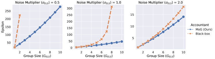
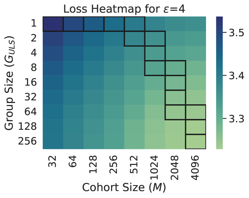
The function in Theorem 1 is easily computable using open-source DP accounting libraries (see Appendix A.1 for a code sample). We use this in Fig. 1 to empirically compare the computed by Theorem 1 to the given by black-box reductions. Our accountant gives near-linear scaling of in in settings whereas generic user-to-example reductions give exponential scaling in . The optimality of our accountant is important for comparing ELS to ULS: if ELS is outperformed by ULS at some fixed user-level -DP guarantee, it is not because of slack in privacy accounting.
Since Algorithm 2 applies a straightforward subsampled Gaussian mechanism, its formal privacy guarantees are well understood and easy to compute [e.g. 28]. In order to directly compare ELS and ULS, we will use the following result, which follows directly from Theorem 1 by setting .
Theorem 2.
For all , Algorithm 2 satisfies user-level DP with
| (3) |
For any , there is a setting where Algorithm 2 does not satisfy user-level DP.
Comparisons under fixed compute budgets. Both Algorithm 1 and 2 are potentially reasonable choices for fine-tuning LLMs with user-level DP. However, the algorithms vary greatly in how they process data, and finding parameters that maximize utility for a given privacy-level may lead to spurious comparisons. Therefore, we focus on their relative performance under a fixed compute budget. This is motivated by practical considerations: the massive size of LLMs often requires tailoring training pipelines to the compute budget, leading to the burgeoning field of scaling laws [29, 30].
For simplicity, we assume the computation cost is equal to the total number of gradient computations. We do not consider the cost of gradient averaging, clipping, and noise generation, nor the cost of communication, though these can affect runtime. The expected per-iteration compute of ELS equals its expected batch size , while that of ULS equals , where is the expected user cohort size (see Algorithm 2).111For ULS, this is only an upper bound as some users may have fewer than examples. Under a compute budget of gradients per iteration, we would thus aim for an expected user cohort size of . DP accounting of ELS and ULS leverages amplification-by-sampling, but we use use shuffling and deterministic in our experiments222As discussed by Ponomareva et al. [31], this practice introduces a possible gap between the reported bounds and the actual level of DP provided by the algorithm as implemented, though it is relatively common practice in the DP literature to date. Recent work of Chua et al. [32] shows there is in fact an actual and unfavorable gap (shuffling can give worse privacy than Poisson sampling), and so while this practice remains reasonable for comparing algorithms, it should not be used to report DP guarantees on actual privacy-sensitive datasets..
3 Understanding ELS and ULS with Lipschitz Losses
We compare ELS and ULS in a simplified setting with Lipschitz losses using their signal-to-noise ratio, i.e., the noise variance per example gradient. This quantity is often heuristically used to tune DP-SGD hyperparameters (e.g. batch size), as it empirically correlates well with learning utility [31, 33].
Consider Algorithms 1 and 2 operating on a user-partitioned dataset , where each user has examples. To meet a compute budget of iterations with gradients per iteration (in expectation), we choose the sampling ratio for ELS and for ULS. The practitioner is free to tune the group sizes . We analyze the impact of this choice.
Suppose the loss is Lipschitz for each . Let be the smallest constants such that
| (4) |
for all . Thus, and respectively bound the norms of the per-example and per-user gradients.333 Note that and are data-dependent. It is a common (albeit non-private) practice to tune the clip norm on the dataset. The problem of privately choosing a clip norm is beyond the scope of this work. We always have by the triangle inequality. For simplicity of analysis, we set the clip norm to and for ELS and ULS respectively, so the operation in Algorithms 1 and 2 is a no-op. Then, the gradient estimates produced by ELS and ULS at step are:
| (5) | ||||
| (6) |
Here, the noise multipliers and are determined by fixing a desired user-level DP guarantee and a number of training steps . Specifically, using Theorems 1 and 2 respectively, we set
These noise multipliers are computable using open-source libraries, see Appendix A.1. If we compare the per-batch noise variances and of updates (5) and (6) respectively, we have,
| (7) |
While (7) is not entirely predictive of the relative performance of ELS and ULS (since they sample data differently), it is a useful way to compare the methods. The ratio of to is quite similar to the notion of gradient diversity [34]. In general, (7) shows that when is sufficiently small when compared to , ULS adds noise with smaller variance than ELS.
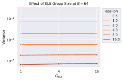
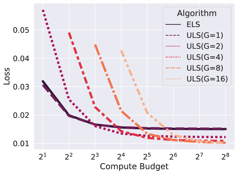
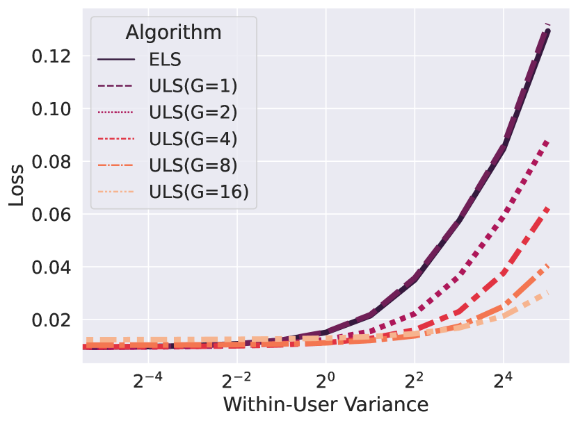
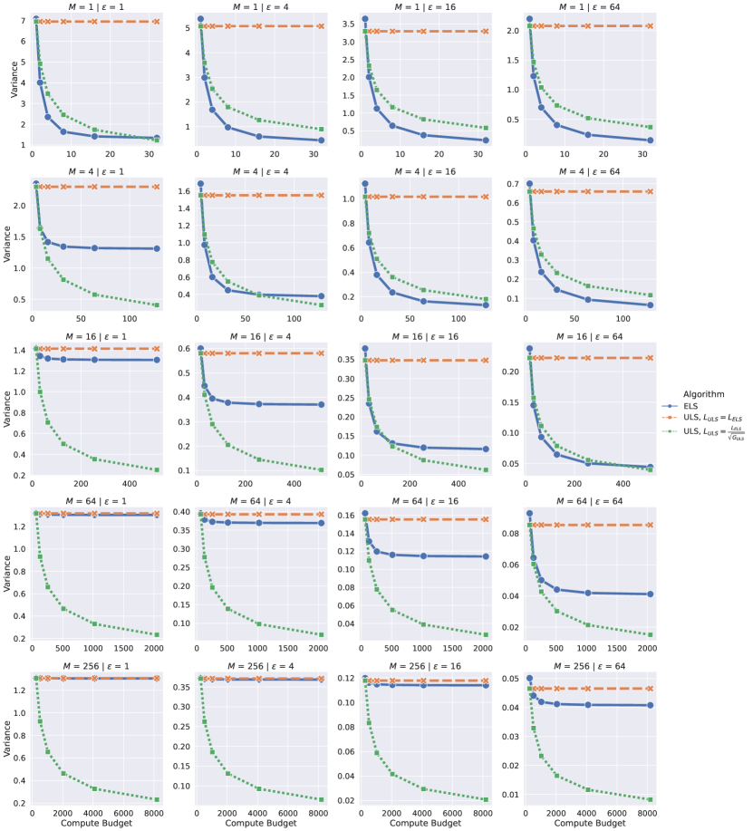
To illustrate this, we plot and in Fig. 2. Fig. 2(a) shows that has almost no effect on the variance . In Fig. 2(b), we see that ULS has smaller variance when (specifically, , that is comparing the blue and green lines) and either is small, or the compute budget is large (and so is large) . Appendix B contains details and more results.
Comparison under maximal group sizes. We now focus on the setting in which where is the maximum user-dataset size. This represents the operating point at which per-example and per-user sampling are maximally different. By construction, in this setting . We conjecture that when , . This is worst-case for ULS, as it means that all gradients within a user point in the same direction. This conjecture is empirically supported by Figures 2 and 9, by comparing variance at the largest compute budget for ELS and ULS with .
Conjecture 1.
Let , and . For all , and , .
While this conjecture is challenging to prove for -DP, we show a weaker version of the conjecture holds for “one-sided” -RDP where is an integer. Recall that for , the -Rényi divergence between distributions is defined by .
Lemma 1.
Let and . For integers , :
To see how Lemma 1 relates to 1, note that the RHS is approximately the Rényi-DP parameter of one iteration of ULS with noise multiplier and the LHS is the Rényi-DP parameter of one iteration of ELS with noise multiplier . Since Rényi divergence is decreasing in the noise multiplier, this implies that there is some such that , so ELS requires a noise multiplier less than times that of ULS to obtain the same Rényi divergence bound. We give the proof in Appendix C. Intuitively, only takes on its extreme values while is more well-concentrated around . Privacy is approximately a convex function of sensitivity, so the latter is better for privacy by Jensen’s inequality.
4 Synthetic Example: Mean Estimation
To better understand the behavior of ELS and ULS, we evaluate them on a mean estimation task with a square distance loss. By focusing on this simple setting, we can thoroughly explore the factors that influence their relative performance, including dataset characteristics, compute budget, privacy budget, and algorithm hyperparameters. In contrast to Section 3, the loss is not Lipschitz.
We first sample a population mean , for . For each of users, we sample a user mean , and user data where . We refer to as the “within-user variance”. Our goal is to estimate under -DP using ELS or ULS. To normalize compute, we set the cohort size in ULS as . We fix and . We use default values of , a per-iterate compute budget of , and , but vary each separately to study how they affect the performance of ELS and ULS. While we vary in all experiments, we find use throughout (as it uniformly gives the best performance for ELS). For each experiment setting, we sweep over learning rate and clip norm, and report the mean loss for the best setting across random trials.
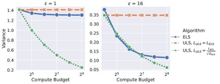
We visualize our results in Fig. 3. We find that ULS with is comparable to if not better than ELS across all settings. We also see that ULS benefits from larger values of when one of the following occurs: (the within-user variance) is large, the compute budget (dictated by the batch size ) is large, or when is small. In these regimes, ULS improves significantly on ELS. We note that the notion that larger values of can improve performance of ULS is corroborated theoretically for Lipschitz losses in Section 3.
5 Language Model Experimental Setup
While Section 3 exhibits conditions under which ULS outperforms ELS for user-level DP training, it is unclear whether this translates into benefits in realistic language model tasks. To investigate this, we apply both to language model fine-tuning, across a variety of privacy and compute budgets.
Model. We use a 350 million parameter decoder-only transformer model, with a WordPiece tokenizer, implemented in Praxis [35]. We use a sequence length of 128, and train via a causal language modeling loss (i.e., next token prediction with cross-entropy loss).
Datasets. For fine-tuning, we use the Stack Overflow and CC-News datasets. Stack Overflow consists of questions and answers from the eponymous social media site, and is directly partitioned into users [36]. The train split has 135,818,730 examples partitioned across 342,477 users. CC-News consists of English language articles on the web. We partition it according to the base domain of each article’s URL. This results in 708,241 examples partitioned across 8,759 users.
For pre-training, we use a modified version of the C4 dataset [37]. Because LLMs can memorize training data [7], we attempt to minimize overlap between C4 and the fine-tuning datasets in order to more accurately reflect the advantages of DP finetuning. As noted by Kurakin et al. [38], overlap between pre-training and fine-tuning may cause us to under-estimate how much DP fine-tuning can improve downstream performance. To remove overlap, we use a two-step filtering scheme: First, we use the NearDup method [39] to identify and remove approximate duplicates between C4 and the fine-tuning datasets. Second, we filter the URLs in what remains, removing all examples associated to stackoverflow.com or URLs contained in CC-News. We refer to the result as C4–. For details, see Appendix D.
Training. We perform non-private pre-training of our transformer model on the C4– dataset. We train for 400,000 steps, using a batch size of 512. We use the Adafactor optimizer [40] with a cosine learning rate decay schedule. We tune the learning rate tuned based on C4 validation set performance. For fine-tuning, we use a dataset-dependent number of steps: 10,000 for Stack Overflow, and 2000 for CC-News. For both ELS and ULS, we use Adafactor with a constant learning rate to perform model updates. We tune the learning rate and clip norm throughout. To decouple the two, we use the normalized clipping scheme proposed by De et al. [21].
DP accounting and sampling. We vary and set , where is the number of examples in the dataset (before any subsampling, as in ELS), following [31, Sec. 5.3.2]. Thus, for Stack Overflow we set , and for CC-News444For CC-News accounting, we make the assumption that there are more users than are actually present in the dataset, due to the smaller number of users. We revisit this choice later on. we set . We compute the noise multiplier assuming amplification via sub-sampling (at the example level for ELS, and at the user level for ULS). For efficiency reasons, in practice we sample by shuffling. For Algorithm 1, we shuffle the dataset and sample batches of a fixed size in shuffled order. For Algorithm 2, we shuffle the set of users and sample user cohorts of a fixed size in shuffled order.
Software and compute resources. We define our model in Praxis [35]. For ELS, we use tf.data pipelines to create and iterate over datasets, and implement Algorithm 1 in JAX. For ULS, we use Dataset Grouper [41] to create and efficiently iterate over users in our datasets. ULS is implemented as a parallelized compute process in FAX [42], enabling linear scaling with respect to compute resources. All experiments were run in PAX [43]. We used TPU v3 pod slices, in , , and topologies for our small, medium, and large compute budget experiments.
6 Language Model Results
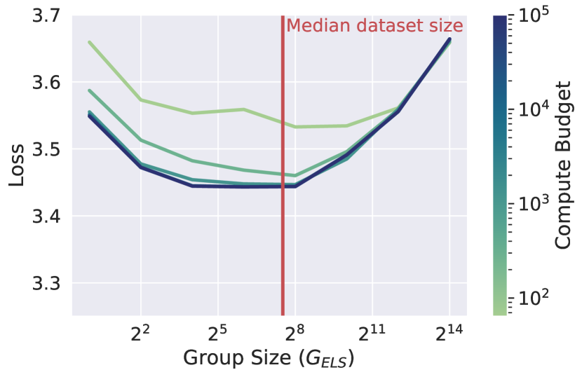
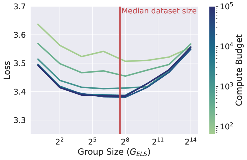
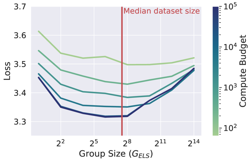
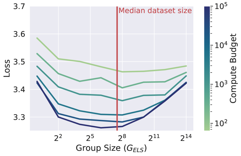
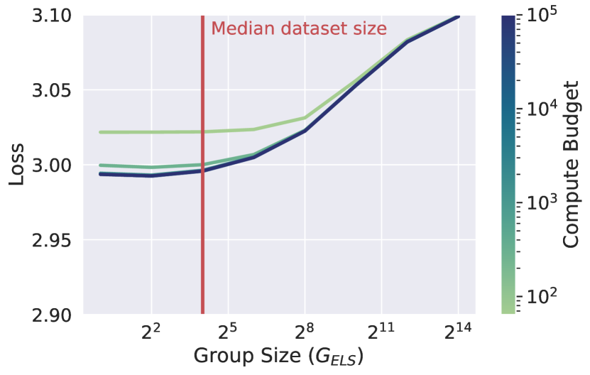
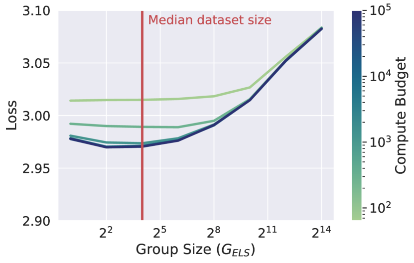
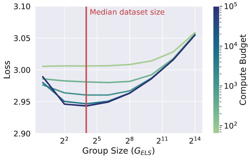
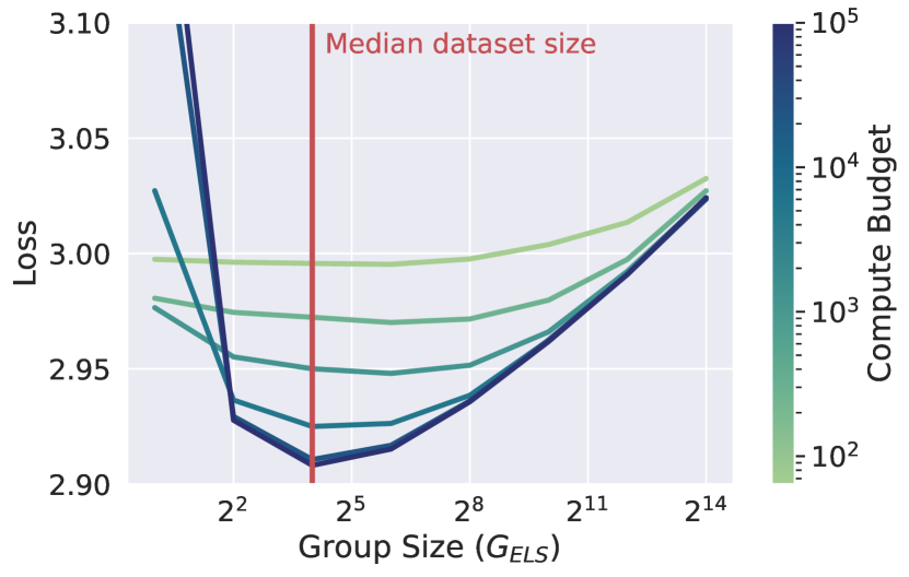
Tuning DP-SGD-ELS. In Algorithm 1, the group size involves a fundamental trade-off: If is small, then the resulting training dataset will be smaller and less diverse, as many clients may have more than examples. However, if is large, then we have to increase the noise multiplier to protect the privacy of users who contribute that many examples, even if most users have fewer than examples. Intuitively, the optimal setting of (in the sense of validation performance subject to a fixed privacy budget) would balance these two competing factors.
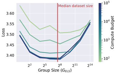
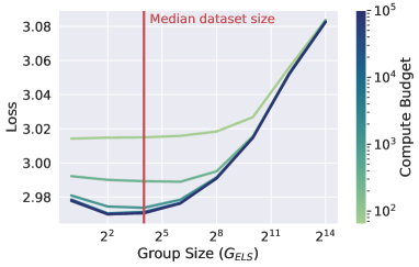
To determine how to tune , we fine-tune via ELS, varying the compute budget and group size , for a variety of . The results for are in Figure 4. We observe a dataset-dependent range of group sizes that work well across compute budgets and . Setting to and works well for Stack Overflow and CC-News, respectively. This coincides almost exactly with the median dataset size across all users. As we show in Appendix E, similar group sizes work across values of . Throughout the remainder, we use this median heuristic to set . This quantity can be approximated well using private median algorithms (see [44], for example).
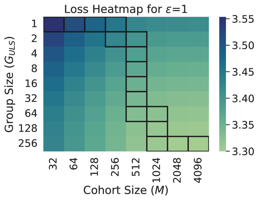
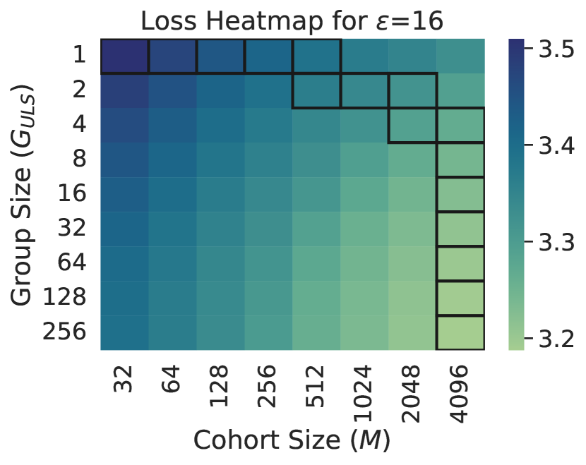
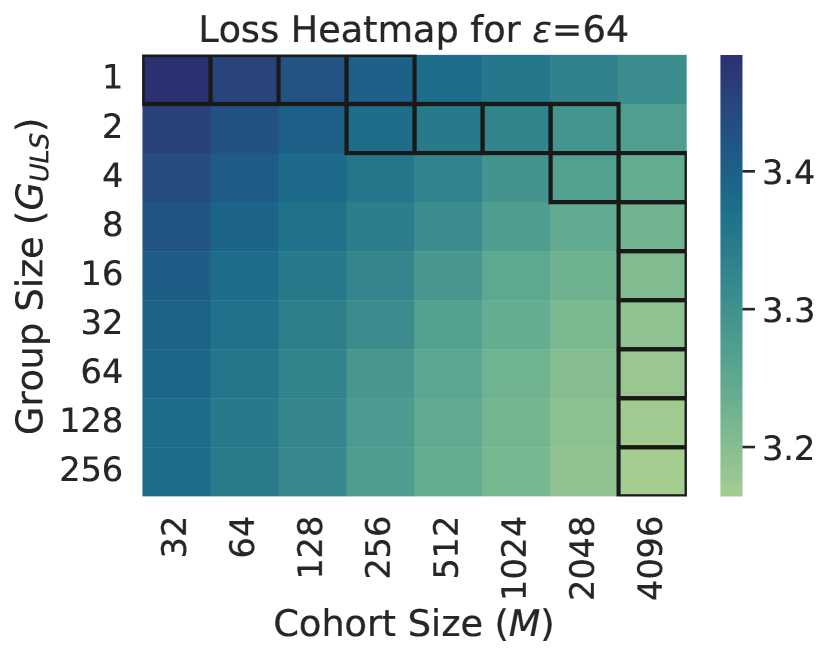
Tuning DP-SGD-ULS. Tuning DP-SGD-ULS requires tuning the group size . Recall that for a compute budget , where is the cohort size. It is a priori unclear how to set these factors for a given compute budget. To understand this, we fine-tune while varying the cohort size , group size , and privacy level . In all experiments, we have some compute budget , and want to figure out how to allocate the compute budget across and so as to minimize validation loss after fine-tuning with privacy budget .
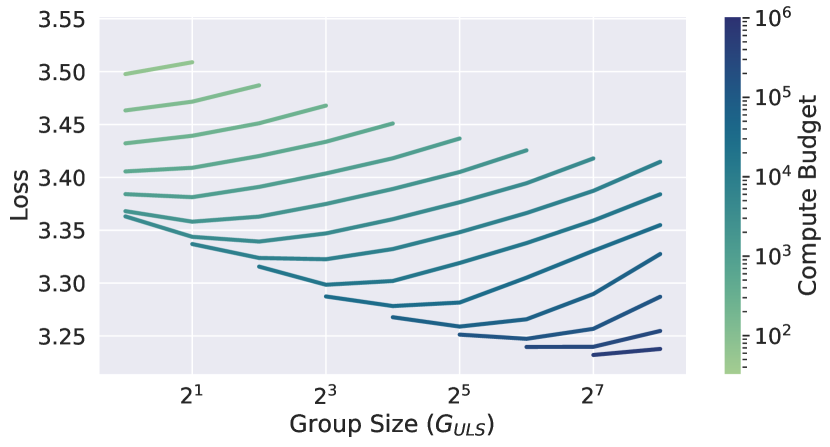
The results for Stack Overflow with are in Figures 5(a) and 5(b). For a given compute budget , it is clearly better to increase up to a limit (in this case 512) before increasing the beyond . For all compute budgets we used, the compute-optimal setting of is always at least an order of magnitude smaller than . By contrast, in federated learning, communication bottlenecks necessitate the use of larger . For example, prior (federated) experiments on Stack Overflow [45, 46, 47, 48] set and , which is far from optimal in our setting; In data-center settings, we get lower loss for approximately the same compute budget by instead setting , .
Recall that by (6), the noise variance is proportional to , where is a the per-user gradient Lipschitz constant, and is the noise multiplier. Increasing reduces by a dataset-dependent factor, while increasing decreases . While is easily computable via (3), can be estimated as follows. Sample a set of users. For each , sample a subset of their dataset of size (at most) , and compute where is the pre-trained model. We estimate ; while (4) suggests using , works well in practice.
We now use the following heuristic for choosing and for a desired compute budget . Start with initial such that . For simplicity, let these all be powers of 2. We compare and . That is, we see whether doubling or will reduce stochastic variance more, and then double whichever reduces variance more. We repeat until . As we show in Appendix F, this strategy is close to optimal in our empirical study. In the rest of our experiments, we set and according to this strategy.
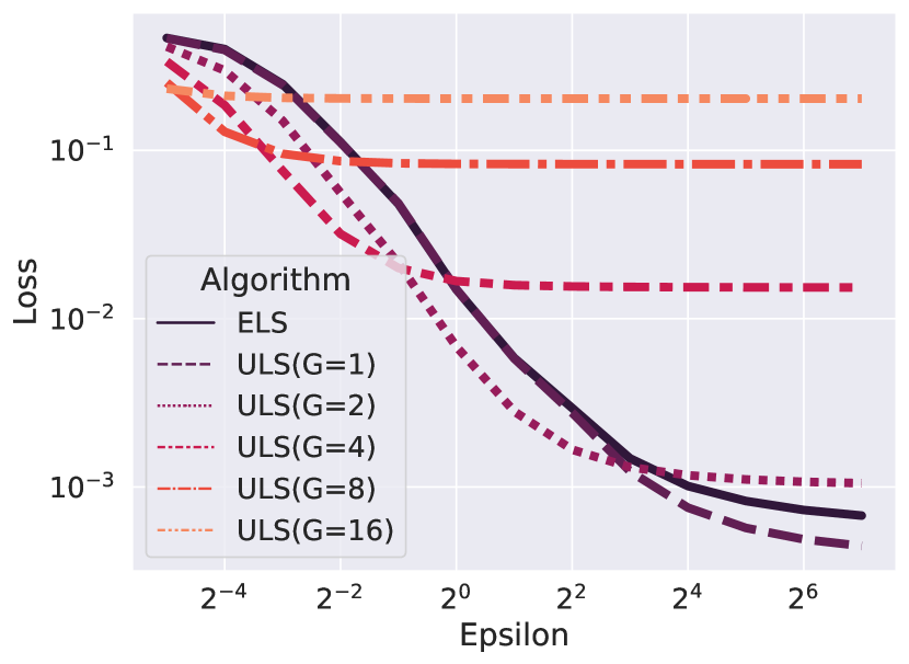
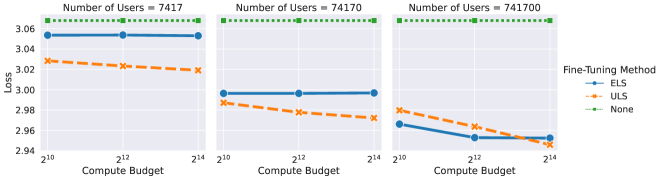
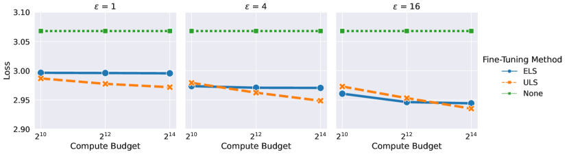
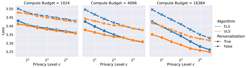
Privacy-utility-compute trade-offs. We now apply ELS and ULS for a variety of compute budgets and values, using the heuristics above to select . We fine-tune on Stack Overflow and CC-News, and compute the test loss on the final iterate. In Figures 6 and 7, we plot privacy-loss trade-offs for three distinct compute budgets. We also compare with using no fine-tuning whatsoever, that is, simply evaluating on the pre-trained checkpoint.
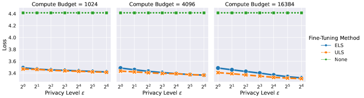
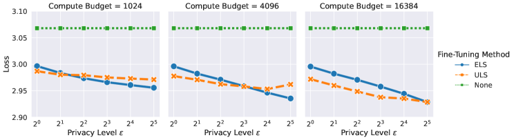
For Stack Overflow, ULS performs at least as well as ELS in all settings. The magnitude of the improvement is largest for small and large compute budgets, aligning with what we observed for simpler settings in Sections 3 and 4. For CC-News, ULS outperforms ELS in many settings, especially when the compute budget is large or is small. For both datasets, ULS improves more with increased compute budgets: if we fix a privacy level , the loss for ULS drops more significantly as the compute budget increases than for ELS. We demonstrate this in greater detail in Section G.1. Notably, fine-tuning with user-level DP provides significant wins over simply using the pre-trained checkpoint in all settings.
Impact of dataset size. We investigate, for a fixed compute budget, how ELS and ULS compare as we vary the number of users. To test this, we use CC-News. We fix all other factors, but vary the number of users only in the privacy accounting. Recall from Section 5 that our results above on CC-News assume there are more users than are actually present, for the accounting. We perform the same experiments, but instead assume there are and more users in the dataset in the accounting. The results for are in Figure 8. Throughout, the loss of ULS decreases more as compute budget increases, but the loss of ELS decreases more as the number of users increases.
Model personalization. In some settings, we may wish to personalize the model after fine-tuning on user data. We measure the ability of the fine-tuned models to personalize to downstream user data. We find that both algorithms seem to benefit comparably from personalization, which does not change the general trade-offs discussed above. For details and results, see Appendix G.2.
7 Related Work
7.1 Comparison to Chua et al. [20]
Concurrently with our work, Chua et al. [20] studied the same algorithms for fine-tuning LLMs with user-level differential privacy. As in our work, they empirically compare the effectiveness of ELS and ULS in datacenter settings. In comparison to our work, [20] focuses on LoRA fine-tuning, compares ELS and ULS to the algorithm of [16], studies the sensitivity of the algorithms to clipping norms, and empirically analyzes various data selection strategies within users. On the other hand, our work expands upon the work of [20] in a few key ways. First, our new accounting techniques enable fairer comparisons between ELS and ULS. Second, the largest dataset [20] uses has 240,173 examples partitioned across approximately 18,000 users, while our experiments encompass a dataset (Stack Overflow) with 135,818,730 examples partitioned across 342,477 users. Third, our comparisons between ELS and ULS normalize on total compute budget, giving us a principled way to compare ELS and ULS as the compute budget changes, which can significantly impact their relative comparison. Last, we provide explicit methodology for selecting the group size in both ELS and ULS, and give extensive empirical evidence for the utility of these methods.
7.2 Theoretical Advances in User-Level DP
Here, we survey the existing theoretical work on user-level DP in various settings.
Reductions to example-level DP. Ghazi et al. [49, 15] give user-level DP bounds by running example-level DP algorithms on subsets of data where the algorithm is stable to deletions ([49] only handles output perturbation while [15] can handle any arbitrary algorithm). This involves a brute-force-search for a stable subset of the data (together with a propose-test-release loop), which can be super-polynomial in the number of examples, and is thus computationally intractable. We note that the user-level DP bounds of [15] rely on generic group privacy reductions [23]. In contrast, we give tight accounting for deriving user-level DP guarantees from example-level DP guarantees in the specific setting of DP-SGD-ELS, enabling us to scale this method to practical LLM settings.
We also note that prior works [50, 51] have also reduced learning with user-level DP to the example-level DP setting where each example is associated with a weight, and the weights are computed to maximize the final utility. On the other hand, we fix a number of examples per user globally and randomly select samples; this can be viewed as assigning a binary per-example weights. It is unclear how to adapt the analytical approaches of [50, 51] to LLMs as we do not have access to utility bounds.
Approaches based on clipping user-level gradients. Several prior approaches rely on bounding user contributions by clipping user-level gradients and combining them with (different choices of) robust mean estimation algorithms [13, 14, 16, 21]. This line of work aims for better rates of convergence under the weaker assumptions. On the other hand, we empirically evaluate practical algorithms derived from these approaches by using user-level gradient clipping but replacing the inefficient robust aggregation approaches with a simple unweighted average (which is efficiently implementable on hardware accelerators).
Simpler theoretical settings. Related work also considers user-level DP in stylized problems such as learning discrete distributions [52] and histograms [53]. Mean estimation under user-level DP was also considered in [54, 55, 56]. This subroutine was also the key building block of the theoretical works [13, 14, 16] in their learning bounds under user-level DP. Continual mean estimation [57] and continual counting [58] have also been considered under user-level DP.
Other related work. Fang and Yi [59] give an approach to privacy amplification from sampling users in a graph structure.
7.3 Federated Learning and User-Level DP
As we noted in the main paper, empirical advances in user-level DP have been driven primarily by research in federated learning, starting with [60, 17, 61, 62]. Specifically, McMahan et al. [17] propose DP-FedSGD (resp. DP-FedAvg) which clips user-level gradients (resp. pseudo-gradients generated by multiple local gradient steps). Note that DP-FedSGD coincides with DP-SGD-ULS that we analyze. This user-level gradient clipping approach can be generalized beyond DP-SGD to algorithms that add noise that is correlated across iterations [46]; these algorithms have been deployed in industrial systems to provide formal user-level DP guarantees [6].
Kato et al. [62] give user-level DP algorithms in a cross-silo federated learning setting. Here, a user’s data might be split across multiple data silos and each silo might contain multiple datapoints from a single user. Their approach combines DP-SGD-ELS with FedAvg, where they use generic group privacy reductions to promote example-level DP guarantees to the user-level.
Several follow-up works have leveraged algorithms similar to DP-SGD-ULS in other settings such as contextual bandits [63], meta-learning [64, 65], and embedding learning [66] as well as applications such as medical image analysis [67], speech recognition [68] and releasing mobility reports (i.e. aggregate location statistics) [69].
8 Discussion
Our work highlights two general findings. First, by introducing tight group-level accounting, we can make ELS a practical method for user-level DP that is scalable to LLM settings and serves as a useful baseline for subsequent research. Second, despite this improvement in accounting, across a wide variety of settings (synthetic and realistic) ULS often outperforms ELS. While we are able to scale ULS to models with hundreds of millions of parameters, ULS uses user-level sampling that is distinct from most LLM training algorithms. Future work is needed to determine which algorithms best balance scalability and performance when training with formal user-level DP guarantees.
Limitations. Despite theoretical advancements in understanding ELS and ULS, we do not have a general theorem comparing their utility across different settings. We also do not provide theoretical comparisons in the absence of Lipschitz loss functions. Empirically, both ELS and ULS depend crucially on group sizes and . While we provide practical heuristics that work well across experiments (Section 6), it is not obvious that these will carry over to all settings of interest. Additionally, due to compute constraints, our work focused on exploring a breadth of hyperparameter configurations rather than on maximally scaling up model size. Determining the model scaling behavior of ELS and ULS is an important topic for future work.
References
- Scao and Rush [2021] Teven Le Scao and Alexander M Rush. How many data points is a prompt worth? arXiv preprint arXiv:2103.08493, 2021.
- Lester et al. [2021] Brian Lester, Rami Al-Rfou, and Noah Constant. The power of scale for parameter-efficient 384 prompt tuning. arXiv preprint arXiv:2104.08691, 282, 2021.
- Bhatia et al. [2023] Kush Bhatia, Avanika Narayan, Christopher M De Sa, and Christopher Ré. Tart: A plug-and-play transformer module for task-agnostic reasoning. Advances in Neural Information Processing Systems, 36:9751–9788, 2023.
- Xi et al. [2023] Zhiheng Xi, Wenxiang Chen, Xin Guo, Wei He, Yiwen Ding, Boyang Hong, Ming Zhang, Junzhe Wang, Senjie Jin, Enyu Zhou, et al. The rise and potential of large language model based agents: A survey. arXiv preprint arXiv:2309.07864, 2023.
- Chen et al. [2019] Mia Xu Chen, Benjamin N Lee, Gagan Bansal, Yuan Cao, Shuyuan Zhang, Justin Lu, Jackie Tsay, Yinan Wang, Andrew M Dai, Zhifeng Chen, et al. Gmail Smart Compose: Real-Time Assisted Writing. In KDD, pages 2287–2295, 2019.
- Xu et al. [2023a] Zheng Xu, Yanxiang Zhang, Galen Andrew, Christopher Choquette, Peter Kairouz, Brendan Mcmahan, Jesse Rosenstock, and Yuanbo Zhang. Federated learning of gboard language models with differential privacy. In Proceedings of the 61st Annual Meeting of the Association for Computational Linguistics (Volume 5: Industry Track), pages 629–639, 2023a.
- Carlini et al. [2021] Nicholas Carlini, Florian Tramer, Eric Wallace, Matthew Jagielski, Ariel Herbert-Voss, Katherine Lee, Adam Roberts, Tom Brown, Dawn Song, Ulfar Erlingsson, et al. Extracting training data from large language models. In 30th USENIX Security Symposium (USENIX Security 21), pages 2633–2650, 2021.
- Carlini et al. [2023] Nicholas Carlini, Daphne Ippolito, Matthew Jagielski, Katherine Lee, Florian Tramer, and Chiyuan Zhang. Quantifying memorization across neural language models. In The Eleventh International Conference on Learning Representations, 2023. URL https://openreview.net/forum?id=TatRHT_1cK.
- Dwork et al. [2006a] Cynthia Dwork, Frank McSherry, Kobbi Nissim, and Adam Smith. Calibrating Noise to Sensitivity in Private Data Analysis. In Proc. of the Third Conf. on Theory of Cryptography (TCC), pages 265–284, 2006a.
- Carlini et al. [2019] Nicholas Carlini, Chang Liu, Úlfar Erlingsson, Jernej Kos, and Dawn Song. The Secret Sharer: Evaluating and Testing Unintended Memorization in Neural Networks. In USENIX Security, pages 267–284, 2019.
- Song and Shmatikov [2019] Congzheng Song and Vitaly Shmatikov. Auditing data provenance in text-generation models. In Proceedings of the 25th ACM SIGKDD International Conference on Knowledge Discovery & Data Mining, 2019.
- Kandpal et al. [2023] Nikhil Kandpal, Krishna Pillutla, Alina Oprea, Peter Kairouz, Christopher A Choquette-Choo, and Zheng Xu. User inference attacks on large language models. arXiv preprint arXiv:2310.09266, 2023.
- Levy et al. [2021] Daniel Levy, Ziteng Sun, Kareem Amin, Satyen Kale, Alex Kulesza, Mehryar Mohri, and Ananda Theertha Suresh. Learning with User-Level privacy. Advances in Neural Information Processing Systems, 34:12466–12479, 2021.
- Bassily and Sun [2023] Raef Bassily and Ziteng Sun. User-level Private Stochastic Convex Optimization with Optimal Rates. In International Conference on Machine Learning, pages 1838–1851. PMLR, 2023.
- Ghazi et al. [2023a] Badih Ghazi, Pritish Kamath, Ravi Kumar, Pasin Manurangsi, Raghu Meka, and Chiyuan Zhang. User-Level Differential Privacy With Few Examples Per User. Advances in Neural Information Processing Systems, 36, 2023a.
- Asi and Liu [2024] Hilal Asi and Daogao Liu. User-level Differentially Private Stochastic Convex Optimization: Efficient Algorithms with Optimal Rates. In International Conference on Artificial Intelligence and Statistics, pages 4240–4248. PMLR, 2024.
- McMahan et al. [2018] H. Brendan McMahan, Daniel Ramage, Kunal Talwar, and Li Zhang. Learning differentially private recurrent language models. In International Conference on Learning Representations, 2018. URL https://openreview.net/forum?id=BJ0hF1Z0b.
- Wei et al. [2021] Kang Wei, Jun Li, Ming Ding, Chuan Ma, Hang Su, Bo Zhang, and H Vincent Poor. User-Level Privacy-Preserving Federated Learning: Analysis and Performance Optimization. IEEE Transactions on Mobile Computing, 21(9):3388–3401, 2021.
- Kairouz et al. [2021a] Peter Kairouz, H Brendan McMahan, Brendan Avent, Aurélien Bellet, Mehdi Bennis, Arjun Nitin Bhagoji, Kallista Bonawitz, Zachary Charles, Graham Cormode, Rachel Cummings, et al. Advances and open problems in federated learning. Foundations and trends® in machine learning, 14(1–2):1–210, 2021a.
- Chua et al. [2024a] Lynn Chua, Badih Ghazi, Yangsibo Huang, Pritish Kamath, Ravi Kumar, Daogao Liu, Pasin Manurangsi, Amer Sinha, and Chiyuan Zhang. Mind the privacy unit! user-level differential privacy for language model fine-tuning, 2024a. URL https://arxiv.org/abs/2406.14322.
- De et al. [2022] Soham De, Leonard Berrada, Jamie Hayes, Samuel L Smith, and Borja Balle. Unlocking high-accuracy differentially private image classification through scale. arXiv preprint arXiv:2204.13650, 2022.
- Abadi et al. [2016] Martin Abadi, Andy Chu, Ian Goodfellow, H. Brendan McMahan, Ilya Mironov, Kunal Talwar, and Li Zhang. Deep Learning with Differential Privacy. In Proceedings of the ACM SIGSAC Conference on Computer and Communications Security, 2016.
- Vadhan [2017] Salil Vadhan. The complexity of differential privacy. Tutorials on the Foundations of Cryptography: Dedicated to Oded Goldreich, pages 347–450, 2017.
- Barthe and Olmedo [2013] Gilles Barthe and Federico Olmedo. Beyond differential privacy: Composition theorems and relational logic for f-divergences between probabilistic programs. In Fedor V. Fomin, Rūsiņš Freivalds, Marta Kwiatkowska, and David Peleg, editors, Automata, Languages, and Programming, pages 49–60, Berlin, Heidelberg, 2013. Springer Berlin Heidelberg. ISBN 978-3-642-39212-2.
- Dwork et al. [2006b] Cynthia Dwork, Krishnaram Kenthapadi, Frank McSherry, Ilya Mironov, and Moni Naor. Our data, ourselves: Privacy via distributed noise generation. In Serge Vaudenay, editor, Advances in Cryptology - EUROCRYPT 2006, pages 486–503, Berlin, Heidelberg, 2006b. Springer Berlin Heidelberg. ISBN 978-3-540-34547-3.
- Balle et al. [2018] Borja Balle, Gilles Barthe, and Marco Gaboardi. Privacy amplification by subsampling: tight analyses via couplings and divergences. In Proceedings of the 32nd International Conference on Neural Information Processing Systems, NIPS’18, page 6280–6290, Red Hook, NY, USA, 2018. Curran Associates Inc.
- Choquette-Choo et al. [2023a] Christopher A Choquette-Choo, Arun Ganesh, Thomas Steinke, and Abhradeep Guha Thakurta. Privacy amplification for matrix mechanisms. In The Twelfth International Conference on Learning Representations, 2023a.
- Koskela et al. [2021] Antti Koskela, Joonas Jalko, Lukas Prediger, and Antti Honkela. Tight differential privacy for discrete-valued mechanisms and for the subsampled gaussian mechanism using FFT. In A Banerjee and K Fukumizu, editors, 24th International Conference on Artificial Intelligence and Statistics (AISTATS), Proceedings of Machine Learning Research, United States, 2021. Microtome Publishing. 24th International Conference on Artificial Intelligence and Statistics (AISTATS) ; Conference date: 13-04-2021 Through 15-04-2021.
- Kaplan et al. [2020] Jared Kaplan, Sam McCandlish, Tom Henighan, Tom B Brown, Benjamin Chess, Rewon Child, Scott Gray, Alec Radford, Jeffrey Wu, and Dario Amodei. Scaling laws for neural language models. arXiv preprint arXiv:2001.08361, 2020.
- Hoffmann et al. [2022] Jordan Hoffmann, Sebastian Borgeaud, Arthur Mensch, Elena Buchatskaya, Trevor Cai, Eliza Rutherford, Diego de Las Casas, Lisa Anne Hendricks, Johannes Welbl, Aidan Clark, et al. Training compute-optimal large language models. arXiv preprint arXiv:2203.15556, 2022.
- Ponomareva et al. [2023] Natalia Ponomareva, Hussein Hazimeh, Alex Kurakin, Zheng Xu, Carson Denison, H. Brendan McMahan, Sergei Vassilvitskii, Steve Chien, and Abhradeep Guha Thakurta. How to DP-fy ML: A Practical Guide to Machine Learning with Differential Privacy. Journal of Artificial Intelligence Research, 77:1113–1201, July 2023. ISSN 1076-9757. doi: 10.1613/jair.1.14649. URL http://dx.doi.org/10.1613/jair.1.14649.
- Chua et al. [2024b] Lynn Chua, Badih Ghazi, Pritish Kamath, Ravi Kumar, Pasin Manurangsi, Amer Sinha, and Chiyuan Zhang. How private are dp-sgd implementations?, 2024b. URL https://arxiv.org/abs/2403.17673.
- Sander et al. [2023] Tom Sander, Pierre Stock, and Alexandre Sablayrolles. TAN Without a Burn: Scaling Laws of DP-SGD. In ICML, pages 29937–29949. PMLR, 2023.
- Yin et al. [2018] Dong Yin, Ashwin Pananjady, Max Lam, Dimitris Papailiopoulos, Kannan Ramchandran, and Peter Bartlett. Gradient diversity: a key ingredient for scalable distributed learning. In International Conference on Artificial Intelligence and Statistics, pages 1998–2007. PMLR, 2018.
- [35] Praxis. https://github.com/google/praxis. Accessed: 2024-05-20.
- Authors [2019] The TensorFlow Federated Authors. TensorFlow Federated Stack Overflow dataset, 2019. URL https://www.tensorflow.org/federated/api_docs/python/tff/simulation/datasets/stackoverflow/load_data.
- Raffel et al. [2020] Colin Raffel, Noam Shazeer, Adam Roberts, Katherine Lee, Sharan Narang, Michael Matena, Yanqi Zhou, Wei Li, and Peter J Liu. Exploring the limits of transfer learning with a unified text-to-text transformer. Journal of machine learning research, 21(140):1–67, 2020.
- Kurakin et al. [2023] Alexey Kurakin, Natalia Ponomareva, Umar Syed, Liam MacDermed, and Andreas Terzis. Harnessing large-language models to generate private synthetic text. arXiv preprint arXiv:2306.01684, 2023.
- Lee et al. [2022] Katherine Lee, Daphne Ippolito, Andrew Nystrom, Chiyuan Zhang, Douglas Eck, Chris Callison-Burch, and Nicholas Carlini. Deduplicating training data makes language models better. In Proceedings of the 60th Annual Meeting of the Association for Computational Linguistics (Volume 1: Long Papers), pages 8424–8445, 2022.
- Shazeer and Stern [2018] Noam Shazeer and Mitchell Stern. Adafactor: Adaptive learning rates with sublinear memory cost. In International Conference on Machine Learning, pages 4596–4604. PMLR, 2018.
- Charles et al. [2023] Zachary Charles, Nicole Mitchell, Krishna Pillutla, Michael Reneer, and Zachary Garrett. Towards federated foundation models: Scalable dataset pipelines for group-structured learning. Advances in Neural Information Processing Systems, 36, 2023.
- Rush et al. [2024] Keith Rush, Zachary Charles, and Zachary Garrett. FAX: Scalable and differentiable federated primitives in jax. arXiv preprint arXiv:2403.07128, 2024.
- [43] Paxml. https://github.com/google/paxml. Accessed: 2024-05-20.
- Tzamos et al. [2020] Christos Tzamos, Emmanouil-Vasileios Vlatakis-Gkaragkounis, and Ilias Zadik. Optimal private median estimation under minimal distributional assumptions. Advances in Neural Information Processing Systems, 33:3301–3311, 2020.
- Denisov et al. [2022] Sergey Denisov, H Brendan McMahan, John Rush, Adam Smith, and Abhradeep Guha Thakurta. Improved differential privacy for SGD via optimal private linear operators on adaptive streams. Advances in Neural Information Processing Systems, 35:5910–5924, 2022.
- Kairouz et al. [2021b] Peter Kairouz, Brendan Mcmahan, Shuang Song, Om Thakkar, Abhradeep Thakurta, and Zheng Xu. Practical and Private (Deep) Learning Without Sampling or Shuffling. In ICML, volume 139, pages 5213–5225, 2021b.
- Choquette-Choo et al. [2023b] Christopher A Choquette-Choo, Hugh Brendan Mcmahan, J Keith Rush, and Abhradeep Guha Thakurta. Multi-epoch matrix factorization mechanisms for private machine learning. In International Conference on Machine Learning, pages 5924–5963. PMLR, 2023b.
- Choquette-Choo et al. [2024a] Christopher A Choquette-Choo, Arun Ganesh, Ryan McKenna, H Brendan McMahan, John Rush, Abhradeep Guha Thakurta, and Zheng Xu. (amplified) banded matrix factorization: A unified approach to private training. Advances in Neural Information Processing Systems, 36, 2024a.
- Ghazi et al. [2023b] Badih Ghazi, Pritish Kamath, Ravi Kumar, Pasin Manurangsi, Raghu Meka, and Chiyuan Zhang. On User-level Private Convex Optimization. In ICML, pages 11283–11299. PMLR, 2023b.
- Amin et al. [2019] Kareem Amin, Alex Kulesza, Andres Munoz, and Sergei Vassilvtiskii. Bounding User Contributions: A Bias-Variance Trade-off in Differential Privacy. In ICML, pages 263–271. PMLR, 2019.
- Epasto et al. [2020] Alessandro Epasto, Mohammad Mahdian, Jieming Mao, Vahab Mirrokni, and Lijie Ren. Smoothly Bounding User Contributions in Differential Privacy. NeurIPS, 33:13999–14010, 2020.
- Liu et al. [2020] Yuhan Liu, Ananda Theertha Suresh, Felix Xinnan X Yu, Sanjiv Kumar, and Michael Riley. Learning discrete distributions: user vs item-level privacy. NeurIPS, 33:20965–20976, 2020.
- Liu et al. [2023] Yuhan Liu, Ananda Theertha Suresh, Wennan Zhu, Peter Kairouz, and Marco Gruteser. Algorithms for bounding contribution for histogram estimation under user-level privacy. In ICML, pages 21969–21996, 2023.
- Girgis et al. [2022] Antonious M Girgis, Deepesh Data, and Suhas Diggavi. Distributed User-Level Private Mean Estimation. In IEEE International Symposium on Information Theory, pages 2196–2201. IEEE, 2022.
- Narayanan et al. [2022] Shyam Narayanan, Vahab Mirrokni, and Hossein Esfandiari. Tight and Robust Private Mean Estimation with Few Users. In ICML, pages 16383–16412, 2022.
- Cummings et al. [2022] Rachel Cummings, Vitaly Feldman, Audra McMillan, and Kunal Talwar. Mean Estimation with User-level Privacy under Data Heterogeneity. NeurIPS, 35:29139–29151, 2022.
- George et al. [2024] Anand Jerry George, Lekshmi Ramesh, Aditya Vikram Singh, and Himanshu Tyagi. Continual Mean Estimation Under User-Level Privacy. IEEE Journal on Selected Areas in Information Theory, 2024.
- Dong et al. [2023] Wei Dong, Qiyao Luo, and Ke Yi. Continual Observation under User-level Differential Privacy. In IEEE Symposium on Security and Privacy, pages 2190–2207. IEEE, 2023.
- Fang and Yi [2024] Juanru Fang and Ke Yi. Privacy Amplification by Sampling under User-level Differential Privacy. Proceedings of the ACM on Management of Data, 2(1):1–26, 2024.
- Geyer et al. [2017] Robin C Geyer, Tassilo Klein, and Moin Nabi. Differentially private federated learning: A client level perspective. arXiv preprint arXiv:1712.07557, 2017.
- Agarwal et al. [2018] Naman Agarwal, Ananda Theertha Suresh, Felix Xinnan X Yu, Sanjiv Kumar, and Brendan McMahan. cpSGD: Communication-efficient and differentially-private distributed SGD. NeurIPS, 31, 2018.
- Kato et al. [2023] Fumiyuki Kato, Li Xiong, Shun Takagi, Yang Cao, and Masatoshi Yoshikawa. ULDP-FL: Federated learning with across silo user-level differential privacy. arXiv preprint arXiv:2308.12210, 2023.
- Huang et al. [2023] Ruiquan Huang, Huanyu Zhang, Luca Melis, Milan Shen, Meisam Hejazinia, and Jing Yang. Federated Linear Contextual Bandits with User-level Differential Privacy. In ICML, pages 14060–14095, 2023.
- Li et al. [2020] Jeffrey Li, Mikhail Khodak, Sebastian Caldas, and Ameet Talwalkar. Differentially private meta-learning. In International Conference on Learning Representations, 2020. URL https://openreview.net/forum?id=rJgqMRVYvr.
- Zhou and Bassily [2022] Xinyu Zhou and Raef Bassily. Task-level Differentially Private Meta Learning. In NeurIPS, 2022.
- Xu et al. [2023b] Zheng Xu, Maxwell Collins, Yuxiao Wang, Liviu Panait, Sewoong Oh, Sean Augenstein, Ting Liu, Florian Schroff, and H Brendan McMahan. Learning to generate image embeddings with user-level differential privacy. In Proceedings of the IEEE/CVF Conference on Computer Vision and Pattern Recognition, pages 7969–7980, 2023b.
- Adnan et al. [2022] Mohammed Adnan, Shivam Kalra, Jesse C Cresswell, Graham W Taylor, and Hamid R Tizhoosh. Federated learning and differential privacy for medical image analysis. Scientific reports, 12(1):1953, 2022.
- Pelikan et al. [2023] Martin Pelikan, Sheikh Shams Azam, Vitaly Feldman, Jan Silovsky, Kunal Talwar, Tatiana Likhomanenko, et al. Federated learning with differential privacy for end-to-end speech recognition. arXiv preprint arXiv:2310.00098, 2023.
- Kapp et al. [2023] Alexandra Kapp, Saskia Nuñez von Voigt, Helena Mihaljević, and Florian Tschorsch. Towards mobility reports with user-level privacy. Journal of Location Based Services, 17(2):95–121, 2023.
- Li et al. [2022] Guoyao Li, Shahbaz Rezaei, and Xin Liu. User-Level Membership Inference Attack against Metric Embedding Learning. In ICLR 2022 Workshop on PAIR2Struct: Privacy, Accountability, Interpretability, Robustness, Reasoning on Structured Data, 2022.
- Miao et al. [2021] Yuantian Miao, Minhui Xue, Chao Chen, Lei Pan, Jun Zhang, Benjamin Zi Hao Zhao, Dali Kaafar, and Yang Xiang. The Audio Auditor: User-Level Membership Inference in Internet of Things Voice Services. In Privacy Enhancing Technologies Symposium (PETS), 2021.
- Chen et al. [2023] Min Chen, Zhikun Zhang, Tianhao Wang, Michael Backes, and Yang Zhang. FACE-AUDITOR: Data auditing in facial recognition systems. In 32nd USENIX Security Symposium (USENIX Security 23), pages 7195–7212, Anaheim, CA, August 2023. USENIX Association. ISBN 978-1-939133-37-3. URL https://www.usenix.org/conference/usenixsecurity23/presentation/chen-min.
- Wang et al. [2019] Zhibo Wang, Mengkai Song, Zhifei Zhang, Yang Song, Qian Wang, and Hairong Qi. Beyond Inferring Class Representatives: User-Level Privacy Leakage From Federated Learning. In IEEE INFOCOM 2019 - IEEE Conference on Computer Communications, page 2512–2520, 2019.
- Song et al. [2020] Mengkai Song, Zhibo Wang, Zhifei Zhang, Yang Song, Qian Wang, Ju Ren, and Hairong Qi. Analyzing User-Level Privacy Attack Against Federated Learning. IEEE Journal on Selected Areas in Communications, 38(10):2430–2444, 2020.
- Jagielski et al. [2020] Matthew Jagielski, Jonathan Ullman, and Alina Oprea. Auditing differentially private machine learning: How private is private SGD? Advances in Neural Information Processing Systems, 33:22205–22216, 2020.
- Pillutla et al. [2023] Krishna Pillutla, Galen Andrew, Peter Kairouz, H Brendan McMahan, Alina Oprea, and Sewoong Oh. Unleashing the Power of Randomization in Auditing Differentially Private ML. NeurIPS, 36, 2023.
- Steinke et al. [2023] Thomas Steinke, Milad Nasr, and Matthew Jagielski. Privacy Auditing with One (1) Training Run. In NeurIPS, 2023.
- Andrew et al. [2024] Galen Andrew, Peter Kairouz, Sewoong Oh, Alina Oprea, H Brendan McMahan, and Vinith Suriyakumar. One-shot Empirical Privacy Estimation for Federated Learning. 2024.
- Choquette-Choo et al. [2024b] Christopher A. Choquette-Choo, Arun Ganesh, Thomas Steinke, and Abhradeep Guha Thakurta. Privacy amplification for matrix mechanisms. In The Twelfth International Conference on Learning Representations, 2024b. URL https://openreview.net/forum?id=xUzWmFdglP.
- Zhu et al. [2022] Yuqing Zhu, Jinshuo Dong, and Yu-Xiang Wang. Optimal accounting of differential privacy via characteristic function. In Gustau Camps-Valls, Francisco J. R. Ruiz, and Isabel Valera, editors, Proceedings of The 25th International Conference on Artificial Intelligence and Statistics, volume 151 of Proceedings of Machine Learning Research, pages 4782–4817. PMLR, 28–30 Mar 2022. URL https://proceedings.mlr.press/v151/zhu22c.html.
- Doroshenko et al. [2022] Vadym Doroshenko, Badih Ghazi, Pritish Kamath, Ravi Kumar, and Pasin Manurangsi. Connect the dots: Tighter discrete approximations of privacy loss distributions. Proceedings on Privacy Enhancing Technologies, 2022:552–570, 10 2022. doi: 10.56553/popets-2022-0122.
- DP Team [2022] DP Team. Google’s differential privacy libraries., 2022. https://github.com/google/differential-privacy.
- McMahan et al. [2017] Brendan McMahan, Eider Moore, Daniel Ramage, Seth Hampson, and Blaise Aguera y Arcas. Communication-efficient learning of deep networks from decentralized data. In Artificial intelligence and statistics, pages 1273–1282. PMLR, 2017.
.1 User-level Privacy Attacks
The work on user-level DP is motivated in part due to the various privacy attacks conducted at the user level. For instance, an adversary might be able to infer whether a user’s data was used to train a model [11], even if the adversary does not have access to the exact training samples of the user [12]. Further, [12] demonstrate that example-level DP is not effective in mitigating such user inference attacks, especially at low false positive rates.
Such attacks have been designed not only for LLMs [12] but also for embedding learning for vision [70], speech recognition for IoT devices [71], facial recognition systems [72]. In federated learning, Wang et al. [73] and Song et al. [74] study the risk to user-level privacy from a malicious server. Such privacy attacks can also be used to audit user-level DP [75, 76, 77] and estimate user-level privacy [78]. User-level DP provides formal upper bounds on the success rates of all such user-level privacy attacks and the algorithms we study are broadly applicable in all of these settings.
Appendix A Tight Accounting for DP-SGD-ELS
Notation. Given a distribution over a space and , let denote the product distribution on .
In this section, we show the following tight accounting statement for Algorithm 1:
Theorem 3.
Let be iterations of DP-SGD-ELS using noise multiplier , loss function , group size , and Poisson sampling with probability . That is, is the distribution of models produced by applying DP-SGD-ELS to a dataset . Let and be two datasets such that where . Then for all :
Furthermore, this is tight, i.e. there exists a loss function and datasets such that:
Since we cap the number of examples any user can contribute to the dataset in Algorithm 1, this implies Theorem 1. To prove this, we use the following lemma from [79], derived using an analysis based on Mixture-of-Gaussians mechanisms:
Lemma 2 (Lemma 4.5 of [79]).
Let be a random variable on , and be a random variable on such that is stochastically dominated by (that is, there is a coupling of and such that under this coupling, with probability 1). Then for all :
We will also use the following “quasi-convexity” property of DP:
Lemma 3.
Let be probabilities summing to 1. Given distributions , let and . Then for any :
Proof.
We have:
is the observation that i.e. “the max of sums is less than the sum of maxes” and holds because the are non-negative and sum to 1. ∎
Finally, we will use the following observation about bijections and hockey-stick divergences:
Observation 1.
Let be any bijection, and for distribution let denote the distribution given by . Then for any :
Proof.
This follows by applying the post-processing property of DP, which says for any function
The observation follows by applying the post-processing property to and . ∎
Proof of Theorem 3.
Since is a bijection (we treat the initialization as public), we can assume through the proof that DP-SGD-ELS instead outputs the tuple . For simplicity of presentation, we will assume is -Lipschitz and thus that is a no-op.
The tightness of this results follows from considering a one-dimensional 1-Lipschitz loss function such that that for all , and for all , . Letting , the distribution of each is exactly for and for .
For the upper bound, we will show
The analogous bound on (and thus the desired bound on ) follows by Lemma 28 of [80].
By adaptive composition of privacy loss distributions (see e.g. Theorem 2.4 of [81]), it suffices to show given any fixed , if are the distribution of conditioned on using and respectively, then for all we have:
Recall that is the set of examples sampled in iteration , and let denote the distributions of respectively conditioned on the event . The distribution of is the same for and , so by Lemma 3 for all :
hence it suffices to show for any fixed and all :
Now let where . We define analogously. The correspondence
is a bijection on , so . We can exactly write the distributions of :
By triangle inequality and -Lipschitzness of , . Furthermore, is distributed according to , and so is stochastically dominated by . By Lemma 2 we now have for all :
which completes the proof. ∎
A.1 Implementation in dp_accounting
A.1.1 Computing and
The following code snippet using the dp_accounting library [82] and scipy methods can be used to compute as a function of (or vice-versa) for DP-SGD-ELS (Algorithm 1) according to Theorem 1, for a given number of steps , example sampling probability , noise multiplier , and group size :
def get_group_level_event(T, p, sigma, K):
    sensitivities = range(K+1)
    probs = [scipy.stats.binom.pmf(x, K, p) for x in sensitivities]
    single_round_event = dp_accounting.dp_event.MixtureOfGaussiansDpEvent(
      sigma, sensitivities, probs
    )
    dp_sgd_event = dp_accounting.dp_event.SelfComposedDpEvent(
      single_round_event, T
    )
    return dp_sgd_event

event = get_group_level_event(T, p, sigma, K)
accountant = dp_accounting.pld.PLDAccountant()
accountant.compose(dp_sgd_event)

# Compute epsilon given delta
print(accountant.get_epsilon(delta))

# Compute delta given epsilon
print(accountant.get_delta(epsilon))
A.1.2 Computing
To figure out the minimum needed to achieve a target -DP guarantee for DP-SGD-ELS (Algorithm 1), we can use dp_accounting’s calibrate_dp_mechanism:
def get_group_level_sigma(T, p, epsilon, delta, K)
    sigma_to_event = lambda sigma: get_group_level_event(T, p, sigma, K)
    return dp_accounting.calibrate_dp_mechanism(
        dp_accounting.pld.PLDAccountant,
        sigma_to_event,
        epsilon,
        delta
    )
Appendix B Comparing Variances of ELS and ULS
Recall that in the setting of Section 3, the stochastic gradients produced by ELS and ULS in an iteration are respectively given by
where denotes the per-iterate (expected) compute budget of both methods, and is the (expected) cohort size of ULS. Further recall that in this setting, there are users, each of which have examples.
For any specific instatiation of this setting, we can use the DP accounting tools from Appendix A to explicitly compute and .
We do so in the following setting. We fix users, each with examples. We set (though the choice here has almost no impact on the noise variance). We vary the cohort size , and set to normalize compute between ELS and ULS. We fix and vary in the desired -DP guarantee, and compute the corresponding noise multipliers via DP accountants.
To compute variance, the only remaining relevant quantities are and . We fix , and vary . Intuitively, the ratio of these two tells us how diverse the gradients across a user are. We consider two settings. In the first, the gradients across a user in ULS are minimally diverse, so that for all group sizes . In the second, the gradients are maximally diverse, so that
This setting occurs, for example, if all gradients computed at each user for ULS are orthogonal with length . For varying and , we then compare three variances: the variance of , and the variance of for each setting of .
The results are given in Fig. 9. While the results vary across settings, we see a few robust findings. First, when , the variance of ELS is lower in nearly all settings. When , the variance of ULS is often (but not always) lower than that of ELS. We see that ULS especially tends to incur lower variance when either (1) is small or (2) when the compute budget is sufficiently large.
Appendix C Proof of Lemma 1
Proof.
Let . By linearity of expectation, we have
This last step follows from the fact that for and , . For , we define random variables , and can write . Let . Then we have:
| (by Jensen’s inequality) | |||
| (by the law of total expectation) | |||
∎
Appendix D Datasets
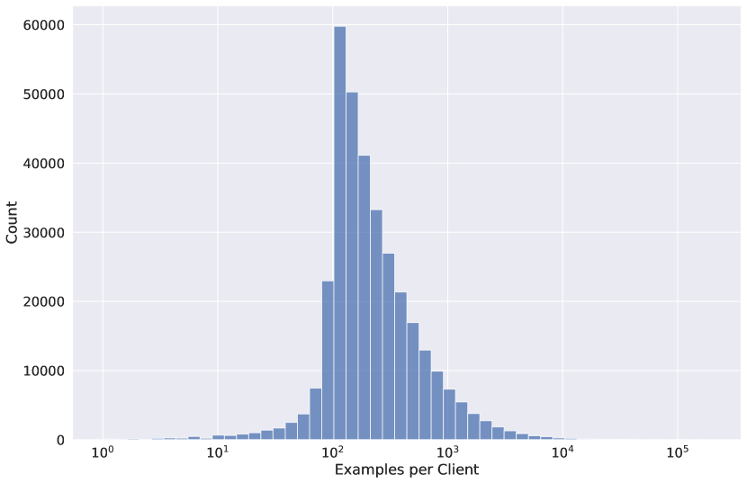
We use two user-partitioned datasets, Stack Overflow and CC-News, for fine-tuning and evaluation. The Stack Overflow dataset [36], consists of questions and answers from stackoverflow.com, and is naturally partitioned by user on the platform. The dataset contains three splits: train (examples before 2018-01-01 UTC), test (examples after 2018-01-01 UTC) and validation (examples from held-out users across time). For our experiments, we use the train split for fine-tuning and the test split for evaluation. Fig. 10 depicts the distribution of user dataset size in the train split. Stack Overflow evaluation metrics reported throughout the main paper are measured on the full test split. In Section G.2, we also include an ablation on model personalization using Stack Overflow test. Personalization is done by using half of each test user’s examples for further fine-tuning and evaluating each personalized model on the reserved half of each test user’s examples.
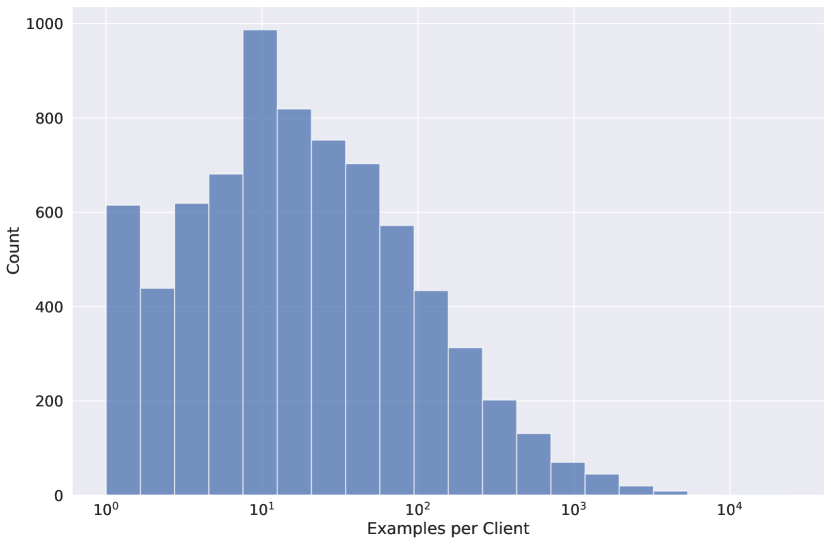
CC-News consists of English-language articles on the web, a subset of the Colossal Clean Crawled Corpus (C4) dataset. For CC-News, we leverage Dataset Grouper to obtain user-level partitioning by base domain of each article’s URL [41]. We reserve a portion of each user’s data in CC-News for evaluation and train on the remainder. In order to do so, we remove all users with only a single example. Eval user datasets are then formed by taking the first 10% of the data of each user, but only up to a maximum of 32 examples. The remaining 90% of user data is allocated for training. Fig. 10 shows the distribution of examples per user in the CC-News training dataset, after the held-out portion of examples are removed. Dataset statistics for Stack Overflow and CC-News are reported in Table 1.
| Dataset | Split | Dataset-level Statistics | User-level Statistics (# examples / user) | |||
| # Examples | # Users | Min | Median | Max | ||
| Stack Overflow | Train | 135.8 M | 342.5 K | 1 | 183 | 194.2 K |
| Test | 16.6 M | 204.1 K | 1 | 43.2 K | 29 | |
| CC-News | Train | 661.6 K | 7.4 K | 1 | 16 | 24.4 K |
| Test | 45.3 K | 7.4 K | 1 | 2 | 32 | |
To create a pre-training dataset with minimal privacy leakage, we start with the C4 dataset [37] and apply de-duplication techniques. First, we apply the approximate duplicate detection method NearDup proposed by Lee et al. [39] to filter out near-duplicates between C4 and the union of Stack Overflow and CC-News. To further remove potential overlap, we filter out all examples associated with stackoverflow.com or any URL in CC-News. This yields the C4– dataset, which we use for pre-training. Statistics of example counts at each stage of the filtering pipeline are reported in Table 2.
| Dataset | Split | # Examples | # Ex, de-duplicated | # Ex, de-duplicated and URL-filtered |
|---|---|---|---|---|
| C4 | Train | 364.6 M | 345.6 M | 325.9 M |
Appendix E Configuring DP-SGD-ELS
In Algorithm 1, governs an important trade-off. Smaller values mean that ELS trains on a small fraction of the dataset, while larger values means that users with more examples are potentially over-represented in sampling. To understand this, we fine-tune on both datasets using ELS, for varying compute budget and group size. The results for Stack Overflow and CC-News are given in Figures 11 and 12. While behavior for boundary values can be quite complicated and dependent on , setting to the median dataset size works well throughout.
Appendix F Configuring DP-SGD-ULS
In Section 6 we discussed the problem of how to set the group size parameter for ULS. We expand on our discussion, and give a heuristic for selecting for a given compute budget. Recall that in Section 3, we showed that the variance of the additive noise in Algorithm 2, which we denote , satisfies , where denotes proportionality, is the maximum per-user gradient norm, and is the noise multiplier. We use as a proxy for downstream performance.
As discussed in Section 3, the quantity is a function of , which we denote . To see this, note that each user-level gradient is an average over (at most) example gradients. If, for example, every user has completely orthonormal example gradients, then . The exact dependence of on is data-dependent, but can be estimated as a function of by computing the norm of user-level gradients across the dataset. We do this as follows. We first sample some set of users. For each user , we randomly select a subset of its dataset of size (at most) . For each such user, we then compute
where is the pre-trained model. Let be some statistical estimator on sets of nonnegative real numbers. We can then approximate
| (8) |
As we discuss in Section 6, we let denote the median, rather than a maximum suggested by (4). The noise multiplier is independent of , but depends on the sampling probability in Algorithm 2. In settings with a fixed cohort size , this means that is a function of , which we denote . We can compute this function via (3) using DP accounting libraries.
Fixing all other parameters of interest (including the desired privacy level ), the variance of the noise added in ULS effectively satisfies the following:
| (9) |
Now, say we have a desire compute budget . To configure ULS, we must select a group size and cohort size such that . By (9), we would like to solve:
| (10) |
While we can compute and at individual points, directly optimizing (10) is challenging. Therefore, we consider a conceptually simpler problem: Suppose we are given some and , such that . If we instead wanted to utilize a compute budget of , should we use the operating point or the operating point ? This can be answered by computing the following quantities:
| (11) |
Intuitively, these represent how much we shrink the objective in (10) by doubling or , respectively. If , then we should double , and otherwise we should double . We formalize this iterative strategy in Algorithm 3, and refer to it as the “Estimate-and-Double” algorithm.
F.1 Validating Algorithm 3
To determine the efficacy of Algorithm 3, we compute the loss of ULS when fine-tuning on Stack Overflow and CC-News, for a variety of group sizes and cohort sizes . We vary these over:
| (12) |

The results for Stack Overflow are given in Fig. 13. We note that the anti-diagonals of the heatmaps represent a fixed compute budget. Using this information, we can now see how close the strategy in Algorithm 3 compares to the optimal setting of and for a given compute budget (over the aforementioned powers of 2 we sweep over). Note that specifically, we initialize with .
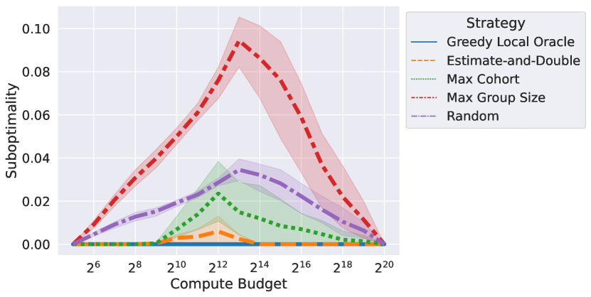
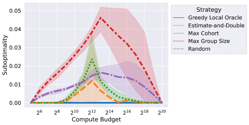
To get a better sense of this, we compute, for compute budgets , the difference in loss between the optimal setting of and , and the following strategies:
-
•
Greedy Local Oracle: Given , this strategy has access to an oracle that can compute the fine-tuning loss when setting , and when setting . It then doubles whichever parameter results in a lower loss. Note that while this is not computationally tractable, it serves as a useful lower bound on the effectiveness of any local strategy.
-
•
Estimate-and-Double: This is the strategy described by Algorithm 3, starting with . We estimate by sampling 128 users at random.
-
•
Random: Given a compute budget , this selects a random from (12) such that .
-
•
Max Cohort: This picks from (12) with a maximum value of such that .
-
•
Max Group Size: This picks from (12) with a maximum value of such that .
The results are given in Figures 14 and 15. Note that suboptimality here refers to the difference in loss between DP-SGD-ULS, when configured using one of the strategies above, versus when it is configured optimally. We see that Algorithm 3 does well across compute budgets and , for both datasets, and performs as well as the oracle strategy for most compute budgets.
Appendix G Additional Experimental Results
G.1 Compute-Loss Trade-offs

In Figures 16 and 17, we present the same information as in Figures 6 and 7 in Section 6, but we instead consider the privacy-compute trade-offs for varying privacy levels . We find that ULS is more capable of improving its performance with increased compute budgets. In light of our analysis above, this makes intuitive sense: ELS can only use increased compute budgets to reduce its noise multiplier , which has diminishing returns. However, ULS can allocate increased compute budgets to reduce its clip norm and its noise multiplier , trading them off as benefits saturate. We see the same effect in Fig. 2.
G.2 Personalizing Fine-Tuned Models
We take models trained via ELS and ULS, and further personalize them to user data. In general, we are interested in whether the two algorithms exhibit different personalization behavior. A priori, this is plausible, as algorithms that operate at a user-level (including FedAvg [83]) can often exhibit improved personalization performance, even on LLM training tasks [41].
To test this, we take our fine-tuned models, and further personalize them on each individual test user’s dataset. We compare models fine-tuned via ELS and ULS on the Stack Overflow dataset, and evaluate their personalization ability on the test users, comparing their performance with and without personalization. We do so by taking the Stack Overflow ELS and ULS checkpoints, and further fine-tuning on individual test user datasets. We perform four local epochs of SGD, with a tuned learning rate, on half of each test users’ examples. We then evaluate the personalized models on the reserved half of each test users’ examples. We record the performance of each model, with and without personalization, on the reserved half of the test users’ examples. The results are in Figure 18.
We see that for both algorithms, personalization seems to incur a uniform reduction in loss. However, the gap between using and not using personalization seems to be roughly the same for both model checkpoints. Personalization does not seem to change the fundamental shape of the trade-off curves. In particular, ULS with personalization seems to outperform or match ELS for the same privacy levels and compute budgets as without personalization.