SvANet: A Scale-variant Attention-based Network for Small Medical Object Segmentation

Abstract

Early detection and accurate diagnosis can predict the risk of malignant disease transformation, thereby increasing the probability of effective treatment. A mild syndrome with small infected regions is an ominous warning and is foremost in the early diagnosis of diseases. Deep learning algorithms, such as convolutional neural networks (CNNs), have been used to segment natural or medical objects, showing promising results. However, analyzing medical objects of small areas in images remains a challenge due to information losses and compression defects caused by convolution and pooling operations in CNNs. These losses and defects become increasingly significant as the network deepens, particularly for small medical objects. To address these challenges, we propose a novel scale-variant attention-based network (SvANet) for accurate small-scale object segmentation in medical images. The SvANet consists of Monte Carlo attention, scale-variant attention, and vision transformer, which incorporates cross-scale features and alleviates compression artifacts for enhancing the discrimination of small medical objects. Quantitative experimental results demonstrate the superior performance of SvANet, achieving 96.12%, 96.11%, 89.79%, 84.15%, 80.25%, 73.05%, and 72.58% in mean Dice coefficient for segmenting kidney tumors, skin lesions, hepatic tumors, polyps, surgical excision cells, retinal vasculatures, and sperms, which occupy less than 1% of the image areas in KiTS23, ISIC 2018, ATLAS, PolypGen, TissueNet, FIVES, and SpermHealth datasets, respectively.

I Introduction

It is essential to detect and diagnose diseases or conditions at their earliest stages, often prior to the manifestation of symptoms. Early detection can aid in the discovery of potential diseases, such as precancerous stages, leading to higher survival rates of patients [1, 2, 3, 4]. For instance, Sung et al. [5] found that the five-year survival rate for melanoma could reach 99% if diagnosed and treated early, compared to only 27% if detected in the late stage. In the early stages of diseases like glaucoma [1], skin cancer [2], colorectal cancer [3], hepatocellular carcinoma [6], renal cancer [4], etc., the affected areas are comparatively small and difficult to detect. The morphometrics of these affected areas is believed to reflect the risk (e.g., cancer precursors) and progression of diseases [1, 2, 3, 6, 4, 7]. Accurately delineating the boundaries of lesions is crucial for their complete resection. Cell-level imaging analysis is also a cutting-edge field with various clinical applications, such as tumor resection analysis [7] and in vitro fertilization [8]. However, examining cells can be challenging due to differences in size, morphology, and density, especially on a small scale.

Figure 1: Architecture of the scale-variant attention-based network (SvANet). Monte Carlo attention (MCAttn) and MCAttn-based bottleneck (MCBottleneck) modules, positioned in the top-left dashed boxes, learn global and local features, respectively. Cross-scale guidance and scale-variant attention (SvAttn) techniques, shown in the top-middle dashed boxes, integrate low-level and high-level feature maps. Convolution with vision transformer by assembling tensors (AssemFormer), located in top-right dashed boxes, synergistically correlates local and global features, combining the strengths of convolutional neural networks and vision transformers.

Various methodologies, including biomarkers, screening programs, medical imaging, genomics, and epidemiology, are commonly used for early disease detection and diagnosis. Recently, deep learning algorithms have demonstrated significant potential in enhancing diagnostic efficiency by reducing costs and interpreting images from various imaging modalities, such as ophthalmoscopy (Oph), dermatoscopy (Derm), colonoscopy (COL), magnetic resonance imaging (MRI), computerized tomography (CT), whole slide imaging (WSI), microscopy (Microsc), electron microscopy (EM), and X-ray [9, 10, 11, 12, 13, 14, 15, 16]. Compared to experienced medical specialists, deep learning algorithms have achieved better or comparable results in medical image segmentation. However, these methods often neglect the small-sized medical objects.

Medical objects that occupy less than 10% of the area pose a significant challenge in medical imaging due to their subtle texture and morphology. Detecting the malignant potential of polyp lesions smaller than 10 mm, for example, is a challenging task [3]. In reality, a large number of images from various modalities contain numerous lesions that occupy less than 10% of the total image area [1, 2, 3, 6, 4, 7], as detailed in Tab. I.

Deep learning algorithms, which employ convolution and pooling, can result in the loss of details for small objects, leading to noticeable compression artifacts. Therefore, it is paramount to develop practical methods for detecting small medical objects. To address the issue of diminished image resolution and information loss, four main strategies have been developed. These strategies include upscaling input data [17], expanding network variants [9, 10, 11, 14, 12, 13, 15, 16], tuning loss functions [18, 19, 15], and post-processing [15]. Most recently, the vision transformer (ViT) has been introduced to process sequences of image patches to learn the inter-patch representations, which has shown noticeable potential in aggregating and preserving the features of small objects [16].

This study presents SvANet, a novel scale-variant attention-based architecture designed to segment medical objects. The primary goal of SvANet is to mitigate disease progression and enable timely interventions. The key contributions of this study are highlighted below:

• We propose SvANet, a new network that utilizes two novel attention mechanisms and a vision transformer to identify small medical objects. To the best of our knowledge, this is the first study to systematically analyze small medical objects across various medical image modalities (i.e., Oph, Derm, COL, MRI, CT, WSI, and Microsc) and diverse object types (i.e., retinal vessels, skin lesions, polyps, livers, kidneys, tumors, tissue cells, and sperms).

• We introduce the Monte Carlo attention (MCAttn) module, which generates attention maps at different scales in a single stage by using agnostic pooling output sizes. MCAttn learns the object relations and spatial information of small medical objects with consideration of both their position and morphology.

• We develop the scale-variant attention (SvAttn) method, which captures the positional and morphological essence of small medical objects by generating attention maps based on the progressively compressed feature maps.

• To further enhance the recognition of small-scale medical objects, we present AssemFormer, a method that combines convolution with a vision transformer by assembling tensors. This approach enables the incorporation of both local spatial hierarchies and inter-patch representations, providing a comprehensive understanding of the image data.

• Equipped with these novel designs, SvANet achieved top-level performance in ultra-small and small medical object segmentation on seven benchmark datasets, outperforming seven state-of-the-art methods. For instance, SvANet achieved the highest mDice of 89.79% and the lowest MAE of 1.6×10^-3 in distinguishing livers and liver tumors that cover less than 1% regions in abdominal slices.

II Related Work

II-A Medical Object Segmentation

Surface structures, shapes, and sizes are critical in characterizing medical objects. The morphometrics are collected by various devices from different patients, making them complex and challenging to analyze. In recent years, deep learning techniques in computer vision have obtained promising performance for medical image segmentation. One widely adopted structure for analyzing medical images is the encoder-decoder-based construction, introduced by Long et al. in 2015 [20]. This approach involves extracting derived features from an encoder and using a decoder to generate the final segmentation mask. Building upon the encoder-decoder structure, Ronneberger et al. [9] introduced “U-shaped” architectures, which connect the limbs by using convolution (UNet) to disseminate information for segmenting tumor cells or general objects. To further enhance the fusion of multi-scale features in analyzing medical images across CT, MRI, and EM modalities, Zhou et al. [10] introduced UNet++, an extension of UNet that incorporates densely connected links.

To improve the performance of encoder-decoder architectures in perceiving medical images, advanced techniques have been suggested. These techniques consists of attention mecahnisms [21], multi network branches [15], contrastive learning [19], and feature interactions [15, 21]. For example, Fan et al. [11] suggested a parallel reverse attention network (PraNet) by integrating an up-sampled feature generated by the medium decoder to discern clearer boundaries of polyps in colonoscopy images. Pan et al. [15] introduced a three-branches “U-shaped” framework to ameliorate feature interactions by post-processing outputs from three branches with the watershed algorithm for examining nuclei. In the study of CT scans of the pancreas, Miao et al. [19] boosted the multi-branch architecture by facilitating contrastive learning and a consistency loss function. When assessing polyps from six unique medical centers, Jha et al. [21] integrated transformer with residual connections of convolution to propagate information from the encoder to the decoder. Despite the promising results achieved by the research above in medical image recognition, one aspect overlooked is the size of medical objects, particularly small-scale objects.

II-B Small Medical Object Segmentation

The convolution and pooling operations in deep learning algorithms compress input data, thus damaging the morphological characteristics of medical objects. To mitigate information loss when reducing image resolution, one common method is to upscale the input images for generating high-resolution feature maps of small objects [17]. However, this method can be time-consuming during training and testing due to the need for image augmentation and feature dimension enlargement. Another promising method is to expand network variants by incorporating techniques such as atrous convolution [22], skip connections [9, 10], feature pyramids [23, 14, 24], multicolumns [25, 14, 13, 15], or attention mechanisms [11, 14, 12, 13, 15, 16], which captures cross-scale features and contributes to magnify small objects. For example, Zhao et al. [23] introduced the pyramid scene parsing network (PSPNet), which employs pyramid pooling and concatenates up-sampled features from multiple scales to improve context feature learning. Lou et al. [12] proposed a context axial reverse attention network (CaraNet) to detect small polyps and brain tumors with less than 5% size ratios. However, CaraNet lacks sufficient interpretability regarding its practicality for segmenting small medical objects, appearing more as a general design suited to the segmentation task.

Designing new loss functions is another practical way to boost small object identification. Guo et al. [18] proposed a loss function that adopts the boundary pixel’s neighbors to enhance the small object segmentation. Besides, Pan et al. [15] combined six different loss functions for nuclei diagnosis. However, the disadvantage of replacing the loss function is that it may not be semantically understandable [18, 19] or it can increase the computational complexity [15]. Post-processing, such as the watershed algorithm [15], can also be employed to enhance small object segmentation. However, post-processing is a distinct step from the segmentation model, and the network cannot adjust its weights to the post-processing results.

Previously, object sizes were quantified by object category [18, 26], number of pixels [17], or size ratio[12] in the images. However, the size of the same object can vary based on the distance between the object and the camera, and computer vision algorithms often resize the entire input image, resulting in changes in pixel numbers. Thus, relying solely on the object category or number of pixels cannot accurately describe the size. This study categorizes medical objects with an area ratio below 1% as ultra-small scale and those below 10% as small scale, which provides a more precise and contextually relevant measure of object size tailored explicitly for medical imaging.

II-C Attention Mechanisms

The attention mechanism is extensively employed in semantic segmentation to prioritize salient features. Various approaches have been proposed to incorporate attention in different ways. Hu et al. [27] applied the squeeze-excitation (SE) method to generate channel attention for learning semantic representations. Zhou et al. [13] employed channel attention to capturing boundary-aware features for enhancing polyp segmentation. To further extract spatial information, Woo et al. [28] combined channel attention with spatial attention in the convolution block attention module (CBAM). Hou et al. [29] further advanced CBAM by introducing coordinate attention (CoorAttn), which utilizes channel-wise average pooling to generate attention maps. Reverse attention is another practical method to mine boundary cues. PraNet [11] extracted fine-grained details by removing the estimated polyps regions using boundary information. Lou et al. [12] enhanced PraNet by decomposing attention maps along height and width axes. Moreover, self-attention is an effective attention scheme to obtain dependencies and relationships within input data. He et al. [30] proposed a fully-transformer-based network that amalgamated spatial pyramid theory and vision transformer to identify skin lesions. However, the vanilla vision transformer lacks inherent bias and is susceptible to perturbations [31]. Zhang et al. [14] and Pan et al. [15] employed self-attention to improve the feature correlations in their CNN-based network for polyps and nuclei examination, respectively. To obtain long-range information when segmenting cell nuclei, Hörst et al. [32] replaced the CNN encoder with a transformer block in the UNet architecture in their CellViT model.

III Methodology

III-A Overall Framework

This section introduces the scale-variant attention-based network (SvANet), specifically designed to segment small medical objects. The SvANet model, schematically depicted in Fig. 1, comprises four main components: Monte Carlo attention in Sec. III-B, cross-scale guidance in Sec. III-C, scale-variant attention in Sec. III-D, and the convolution with vision transformer in Sec. III-E.

Human eyes examine objects by altering the shape of crystalline lenses, thereby creating a detailed visual construction of the object’s characteristics. When viewing an object at various distances, changes in the lens enhance the capture of object details (as per SvAttn and AssemFormer) and changes in location behaviors (as per cross-scale guidance and SvAttn). Drawing inspiration from this phenomenon, we present SvANet by integrating MCAttn, cross-scale guidance, SvAttn, and AssemFormer to mitigate compression defects and enhance the analysis of small medical objects.

To improve the identification of small medical objects and maintain the plug-and-play design of the encoder division, a Monte Carlo attention (MCAttn) based bottleneck (MCBottleneck) is integrated into each encoder stage, depicted by the blue arrows and the blue dashed block in Fig. 1. Preserving the features of tiny medical objects, such as sperms and retinal vessels, becomes challenging after multiple pooling or strided convolution operations. In this study, cross-scale feature maps are applied to guide the latter stages in learning features of small medical objects, represented by the orange arrows in Fig. 1. To improve the identification of object features and their correlations, the correlated features are further processed by convolutions integrated with transformers (i.e., green blocks in Fig. 1). To better comprehend the role of MCAttn, cross-scale guidance, and SvAttn in small medical object segmentation, we examined the feature maps as presented by Fig. 2 and Fig. 3. Due to page limitations, we selected FIVES, ISIC 2018, KiTS23, and SpermHealth as example datasets in Fig. 2 and Fig. 3. To simplicity, we chose to present the outputs from MCBottleneck in stage four and two cross-scale guidance in Fig. 2 and Fig. 3.

Additionally, in Fig. 1, each Conv3×3↓2, represented by black blocks, contains a single 3×3 convolution with a stride of 2 (strided convolution). Every TConv3×3↓2, denoted by grey blocks, consists of three convolution units: a 1×1 convolution, a 3×3 transposed strided convolution, and a 1×1 convolution. Besides, each MCBottleneck consists of a 3×3 convolution, a 1×1 convolution, and an MCAttn module (see Sec. III-B), followed by a 1×1 convolution and an AssemFormer block (see Sec. III-E). The MCBottleneck serves as a compression point in the network, narrowing the tensor channels before expanding them to extract salient features by compressing the input information, resembling a “bottleneck” in information theory. To expand the receptive field and capture features at multiple scales, atrous spatial pyramid pooling (ASPP) [22] is integrated after the final stage of our model.

III-B Monte Carlo Attention

Inspired by this phenomenon, the Monte Carlo attention (MCAttn) module uses a random-sampling-based pooling operation to generate scale-agnostic attention maps. This enables the network to capture relevant information across different scales, enhancing its ability to identify small medical objects.

Figure 2: Output feature maps from MCBottleneck without or with an attention mechanism. (a) Input image, (b) ground truth, and feature map generated (c) without using attention mechanism and with using (d) SE, (e) CBAM, (f) CoordAttn, and (g) Monte Carlo attention (MCAttn). Example images in odd and even rows include ultra-small and small medical objects, respectively.

In Fig. 1, the MCAttn, as presented by the purple block, generates attention maps by randomly selecting a 1×1 attention map from three scales: 3×3, 2×2, and 1×1 (pooled tensors). In conventional methods such as squeeze-excitation (SE), global-average pooling is used to acquire a 1×1 output tensor, which helps calibrate the inter-dependencies between channels [27]. However, this approach has limited capacity to exploit cross-scale correlations. To address this limitation, MCAttn calculates the attention maps from features across three scales, thereby enhancing long-range semantic interdependences. Given an input tensor, $x$, the output attention map of MCAttn, denoted as $\mathcal{A}_{\text{m}}(x)$, is computed as follows:

$$\mathcal{A}_{\text{m}}(x)=\sum_{i=1}^{n}P_{1}(x,i)f(x,i)$$ (1)

where $i$ denotes the output size of the attention map, and $f(x,i)$ represents the average pooling function. The association probability $P_{1}(x,i)$ satisfies the conditions $\sum_{i=1}^{n}P_{1}(x,i)=1$ and $\prod_{i=1}^{n}P_{1}(x,i)=0$, ensuring the generation of agnostic and generalizable attention maps. $n$ represents the number of output pooled tensors and is set to 3 in this study.

The Monte Carlo sampling method described in Eq. 1 allows for the random selection of association probabilities, enabling the extraction of both local information (e.g., angle, edge, and color) and context information (e.g., whole image texture, spatial correlation, and color distribution). In Fig. 2c, the second to the fourth rows and the final row illustrate that MCBottleneck, without using a attention mechanism, struggles to detect the retinas and nevi and often overlooks several sperms. Conversely, when attention mechanisms like SE, CBAM, and CoordAttn are used, localization of densely occupied regions (e.g., optic disc, kidneys, and sperms) is enhanced compared to when no attention mechanism is used. However, sparse regions, such as retinal vasculatures and nevus centres, are often underlooked, especially the ultral-small ones, as shown in Fig. 2c-f. Instead, using MCAttn in MCBottleneck, as depicted in Fig. 2cg, enhances the discernibility of the morphology and precise location of both ultra-small and small medical objects compared to when MCAttn is not used. For instance, in Fig. 2, moving downwards, MCBottleneck coupled with MCAttn emphasizes more apparent retinal vessels for glaucoma, sharper boundaries of nevi, and more perceptible morphology of kidneys, cysts, and sperms. MCAttn also accentuates other medical objects of interest, such as retinas, nevi, kidneys, and sperms, as shown in Fig. 2g.

III-C Cross-scale Feature Guidance

The information content decreases significantly as the size of the medical object reduces, owing to compression artifacts in neural networks. This study introduces a cross-scale guidance module to leverage the higher-resolution features from earlier model stages. Assume that $t$ is the target stage, the output $y_{t}$ can be computed as follows:

$$y_{t}=\sum_{s=1}^{t-1}g(x_{s},t)$$ (2)

where ${x_{s}}$ represents the input tensor in stage $s=1,2,...,t-1$ and the transformation $g(x_{s},t)$ involves $(t-s)\ 3\times 3$ strided convolutions. The function is depicted by the orange arrows and the top-middle orange blocks in Fig. 1.

As illustrated in Fig. 3cd or ef, the highlighted region expands as the input stage increases for the same target stage, $t=4$. This expansion occurs due to an increased total number of strided convolution operations performed on the data.

III-D Scale-variant Attention

The concept of cross-scale feature guidance is based on convolution operations, which have inherent limitations in processing global feature representations. While global pooling operations can facilitate learning context representations, it is restricted to handling features in a uniform scale manner. Given a subregion $x_{j}$ of an input tensor $x$, the output of vanilla global attention, denoted as $\mathcal{A}(x)$, is calculated as follows:

$$\mathcal{A}(x)=\frac{1}{\sigma(x)}\sum_{j=1}^{n}x_{j}$$ (3)

where $x_{j}$ represents the $r^{2}$ neighbourhood centered at the $j^{\text{th}}$ subregion of $x$. Here, $n$ denotes the total number of subregions, and $\sigma(x)$ represents the scalar function that normalizes the result. For vanilla global attention, the default values are set such that $r=1$ and $n=\sigma(x)=H_{x}\times W_{x}$.

Figure 3: Output feature maps from cross-scale guidance without or with scale-variant attention (SvAttn). (a) Input image and (b) ground truth. The feature maps are generated without using SvAttn in (c) $s=1,t=4$ and (d) $s=3,t=4$, and with using SvAttn in (e) $s=1,t=4$ and (f) $s=3,t=4$. Example images in odd and even rows include ultra-small and small medical objects, respectively.

Conventional global attention, as described in Eq. 3, fails to capture relationships across subregions and is limited to computing a single-scale size of the feature. To overcome this scale limitation while maintaining long-range correlations, we introduce scale-variant attention (SvAttn), which processes global dependencies across diverse scales, as depicted by the yellow block in Fig. 1. In SvAttn, multi-scale attention maps are calculated across input stages $s=1,2,...,t-1$. Assuming that the group-wise correspondence among input tensors is controlled by a probability $P_{2}(x)$, the output attention map of SvAttn is defined as:

$$\mathcal{A}_{t}({\bf x})=\frac{1}{\sigma({\bf x})}\sum_{j=1}^{n}\sum_{s=1}^{t-1}P_{2}(x_{s,j})x_{s,j}$$ (4)

where $x_{s,j}$ denotes the $j^{\text{th}}$ subregion of the input tensor at the $s^{\text{th}}$ stage, $t$ is the target stage, and ${\bf x}=[x_{1},x_{2},...,x_{t-1}]^{-1}$ represents the vector of input tensors across various stages. Besides, the correspondence probability $P_{2}(x)$ satisfies the conditions $\sum_{s=1}^{t-1}P_{2}(x_{s},j)=1$ and $\prod_{s=1}^{t-1}P_{2}(x_{s},j)=0$, thereby ensuring a weighted sum of attention maps across different scales. The scalar function $\sigma({\bf x})$ is defined by:

$$\sigma({\bf x})=n=\frac{H\lor W}{2^{t+1}}$$ (5)

where H and W are the height and width of the input image, respectively.

In conjunction with Eq. 2 and Eq. 4, the output tensor $y_{t}^{{}^{\prime}}$ of cross-scale guidance using SvAttn can be defined as follows:

$$y_{t}^{{}^{\prime}}=\mathcal{A}_{t}({\bf x})y_{t}$$ (6)

As indicated by Eq. 4, the subregions located at the same proportional scaling position across stages are dynamic. This variability enables the cross-scale guidance module to effectively discern the relationships between the high-level and low-level features. Consequently, SvAttn enhances the network’s capability to recognize downsized small medical objects throughout a sequence of stages. As illustrated in Fig. 3ce and df, for the same source and target stages, the features captured using SvAttn are more detailed and comprehensive for both ultra-small and small medical objects compared to those obtained without using SvAttn. For example, from top to bottom, there is a more precise delineation of networked retinal vessels, more discernible morphology of nevi, more pronounced instance boundaries of organs such as kidneys, and finer details in sperm morphology. In contrast, without using SvAttn, critical features such as retinal vessels of glaucoma in the first and second rows, the nevus in the third row, and the kidneys and cyst in the sixth rows were overlooked. It is noteworthy that ultral-small objects are harder to perceive compared to small objects without using SvAttn. For example, moving downwards from the odd rows of Fig. 3cd, no retinal vessel were discovered, a relatively small nevus region was highlighted, and the left kidney was missed.

III-E Convolution with Vision Transformer

The proposed convolution with vision transformer by assembling tensors, termed AssemFormer, is illustrated in top-right dased green boxes in Fig. 1. Inspired by [33, 16], AssemFormer incorporates a 3×3 convolution and a 1×1 convolution, followed by two transformer blocks and two convolution operations. AssemFormer bridges convolution and transformer operations by stacking and unstacking feature maps. Equipped with this design, AssemFormer tackles the issue of lacking inductive biases for the vanilla transformer.

The functionalities of convolution and transformer operations differ. Convolution operations focus on learning local and general features, such as corners, edges, angles, and colors of medical objects. In contrast, the transformer module extracts global information, including morphology, depth, and color distribution of medical objects, utilizing multi-head self-attention (MHSA). In addition, the transformer module also learns positional associations of medical objects, such as the relationships between a tumor and the kidney, a kidney and the abdomen, and a tumor and the abdomen within an MRI slice image. The vision transformer algorithm employs a sequence of MHSA and multilayer perceptron (MLP) blocks, each followed by layer normalization [31]. The self-attention mechanism [34] is formulated as follows:

$$\mathcal{A}_{\text{ViT}}(\mathbb{q},\mathbb{k},\mathbb{v})=\text{softmax}(\frac{\mathbb{q}\mathbb{k}^{T}}{\sqrt{D_{\text{h}}}})\mathbb{v}$$ (7)

where $\mathbb{q}$, $\mathbb{k}$, and $\mathbb{v}$ are the query, key, and value vectors of an input sequence $\mathbb{z}\in\mathbb{R}^{N\times D}$. $N$ denotes the number of patches, and $D$ represents the patch size. Given $m$ self-attention operations, $D_{\text{h}}$, the dimension of $\mathbb{q}$ and $\mathbb{k}$, is defined as $D/m$.

Furthermore, a skip connection and concatenation are incorporated to mitigate the information loss concerning small medical objects. Leveraging the convolution-transformer hybrid structure, the AssemFormer block can simultaneously learn the local and global representations of an input medical image. According to the ablation study presented in the fifth and sixth rows of Tab. IV, the AssemFormer significantly improves the segmentation performance of SvANet.

IV Experimental Results

IV-A Evaluation Protocol

IV-A1 Dataset

To validate the effectiveness of SvANet, we conducted tests alongside seven state-of-the-art (SOTA) models for small medical object segmentation across seven benchmark datasets: FIVES [1], ISIC 2018 [2], PolypGen [3], ATLAS [6], KiTS23 [4], TissueNet [7], and SpermHealth.

The FIVES dataset comprises 800 fundus photographs taken with ophthalmoscopes featuring age-related macular degeneration, diabetic retinopathy, glaucoma, and health fundus types. The ISIC 2018 dataset includes skin lesion images collected by dermatoscopes, encompassing both healthy and unhealthy skin areas. PolypGen, sourced from six different hospitals using colonoscopes, focuses exclusively on polyps. The ATLAS dataset consists of 90 MRI scans of livers, detailing two types of medical objects: the liver and tumor. KiTS23 has 599 CT scans of kidneys, categorized into three semantic classes (i.e., kidney, tumor, and cyst). For experimental comparisons, the ATLAS and KiTS23 datasets were sliced into sequences of 2-D images. In addition, TissueNet includes images of cells from the pancreas, breast, tonsil, colon, lymph, lung, esophagus, skin, and spleen, derived from humans, mice, and macaques, collected using cell imaging platforms such as CODEX and CyCIF, with annotations for whole cells and their nuclei.

SpermHealth is a customized dataset from the Prince of Wales Hospital in Hong Kong consisting of low-resolution sperm images (640×480, 96 DPI) extracted from microscope-captured videos. These images have been meticulously annotated into normal and abnormal categories by experienced fertility doctors. Further details of the datasets used in the tests are presented in Tab. I.

TABLE I: Dataset details: medical objects within each dataset are categorized by area ratios: below 1% (ultra-small), below 10% (small), and below 100% (all).

		Number of		Number of object
	Image	image		ultra
Dataset	capture	(train + test)	Object area ratio	small	small	all
FIVES [1]	Oph	600 + 200	0.351% $\sim$ 52.020%	4	145	798
ISIC 2018 [2]	Derm	2594 + 100	0.288% $\sim$ 98.575%	52	1084	2694
PolypGen [3]	COL	1230 + 307	0.003% $\sim$ 85.850%	81	895	1411
ATLAS [6]	MRI	997 + 249	0.001% $\sim$ 25.826%	274	1084	1464
KiTS23 [4]	CT	1703 + 426	0.001% $\sim$ 13.790%	665	1533	1539
TissueNet [7]	WSI	2580 + 1324	0.002% $\sim$ 9.836%	9096	9437	9437
SpermHealth	Microsc	118 + 30	0.042% $\sim$ 0.651%	1456	1456	1456

IV-A2 Implementation Details and Evaluation Metric

In this study, the mini-batch size was set to 4. Data augmentation strategies applied to pre-process the input images included random horizontal flips, random cropping to a resolution of 512×512, Gaussian blur, distortion, and rotation. The AdamW optimizer [35] and a cross-entropy loss function were utilized, with the learning rate decaying from 5×10^-5 to 1×10^-6 following a cosine schedule [36]. The total training process spanned 100 epochs. The results were calculated by averaging the outcomes from three times of training and testing cycles.

The experiments were conducted on an RTX 4090 GPU with an AMD Ryzen 9 7950X CPU. The metrics used to assess the performance of semantic segmentation include the mean Dice coefficient (mDice), mean intersection over union (mIoU), mean absolute error (MAE), sensitivity, and F2 score.

IV-B Results for Datasets with Diverse Object Sizes

The experimental results for the FIVES, ISIC 2018, PolypGen, ATLAS, KiTS23, and TissueNet datasets are summarized in Tab. II. These results demonstrate that SvANet outperforms other SOTA methods across all metrics for ultra-small and small medical object segmentation across six datasets tested.

As presented in Tab. II, SvANet outperformed other SOTA methods across three object scales in the FIVES, ISIC 2018, and ATLAS datasets, excluding sensitivity of 93.54% & 87.13% in ISIC 2018 & ATLAS datasets and MAE of 5.35×10^-4 & 0.66×10^-4 in FIVES & ATLAS datasets for the “all” object scale, as summarized in Tab. II. Additionally, SvANet surpasses other methods with increments in the mDice of +2.95% & +5.23%, mIoU of +2.36% & +5.78%, sensitivity of +0.19% & +5.03%, and F2 score of +1.28% & +5.15% for differentiating ultra-small and small retinal vessels in the FIVES dataset. However, the MAE is comparatively high ($>$75×10^-4) in ultra-small retinal vasculature segmentation across all tested models, potentially due to the minimal number (4) ultra-small objects providing insufficient learnable features for deep learning algorithms. In ISIC 2018 and ATLAS datasets, SvANet excelled in segmenting ultra-small objects (i.e., skin lesions, livers, and hepatic tumors) with mDice of 96.11% & 89.79%, mIoU of 92.76% & 86.06%, sensitivity of 98.35% & 86.68%, and F2 score of 97.42% & 87.71%. These results suggest significant potential for SvANet in diagnosing dermatological skin lesions and hepatic tumors in MRI scans, particularly for objects with an area ratio smaller than 1% or 10%. Thus, SvANet can ameliorate therapeutic approaches such as excision therapy, laser therapy, electrosurgery, and radiotherapy for treating these conditions.

Figure 4: Segmentation mDice across different area ratios of medical objects in (a) FIVES, (b) ISIC 2018, (c) PolypGen, (d) ATLAS, (e) KiTS23, and (f) TissueNet datasets. The legends used in these subfigures are consistent with those detailed in the final panel (f).

Furthermore, the segmentation results for the PolypGen and KiTS23 datasets demonstrate that SvANet delivers superior performance than other SOTA methods across three object scales. Specifically, SvANet achieved the highest mDice of 84.15% & 96.12%, 91.17% & 94.01%, and 93.16% & 94.54% for ultra-small, small, and all medical object scales in PolypGen and KiTS23 datasets, respectively. Moreover, SvANet delivered up to 14.83% & 1.22%, 6.23% & 2.80%, and 6.93% & 2.70% increments in F2 score over other tested methods for ultra-small, small, and all object scales in PolypGen and KiTS23 datasets, separately. The F2 score, the harmonic mean of sensitivity and precision, underscores the robustness of SvANet in medical object segmentation. SvANet also recorded the lowest MAE, 1.01×10^-4 & 0.02×10^-4, 0.66×10^-4 & 0.07×10^-4, and 0.81×10^-4 & 0.08×10^-4 across three object scales for PolypGen and KiTS23 datasets, indicating a high level of precision in the pixel-level recognition of polyps, kidneys, renal tumors, and cysts.

TABLE II: Quantitative results in FIVES, ISIC 2018, PolypGen, ATLAS, KITS23, and TissueNet datasets, divided by area ratios of medical objects: below 1% (ultra-small), below 10% (small), and below 100% (all). The best results are underlined in bold.

		mDice			mIoU			MAE (×10-4)			Sensitivity			F2 score
		ultra			ultra			ultra			ultra			ultra
	Methods	small	small	all	small	small	all	small	small	all	small	small	all	small	small	all
FIVES	UNet (MICCAI’15) [9]	67.49	72.99	71.12	62.54	65.04	63.10	84.65	14.64	6.22	63.86	71.48	70.13	65.06	72.02	70.42
	UNet++ (TMI’19) [10]	70.10	74.46	70.72	65.06	66.37	62.68	80.64	14.46	5.92	67.02	73.05	69.50	68.08	73.58	69.90
	HRNet (TPAMI’20) [25]	69.46	79.16	75.66	64.67	70.83	67.04	88.84	15.38	5.51	68.33	78.30	74.09	68.68	78.60	74.67
	PraNet (MICCAI’20) [11]	64.47	71.46	68.57	59.42	63.08	60.14	79.64	14.78	5.45	61.20	67.88	65.61	62.27	69.11	66.58
	HSNet (CBM’22) [14]	51.55	54.32	51.60	50.37	50.63	48.15	83.00	15.67	4.54	51.56	53.85	51.93	51.55	53.95	51.66
	CFANet (PR’23) [13]	69.35	76.64	72.23	63.16	68.60	65.27	80.18	15.16	4.92	64.86	75.67	73.79	66.29	75.99	72.75
	TransNetR (MIDL’24) [21]	67.87	80.68	78.60	63.59	72.55	69.66	83.54	14.44	5.68	66.90	78.83	77.24	67.26	79.45	77.60
	SvANet (Ours)	73.05	85.91	86.29	67.03	78.33	78.39	76.82	14.42	5.35	68.52	83.86	85.15	69.96	84.60	85.46
ISIC 2018	UNet (MICCAI’15) [9]	87.22	89.82	91.10	81.14	82.75	83.93	62.99	11.28	6.91	97.49	93.75	90.64	91.92	92.05	90.82
	UNet++ (TMI’19) [10]	81.10	88.80	90.73	72.61	81.20	83.30	93.65	12.59	7.35	98.29	93.64	91.06	89.12	91.54	90.92
	HRNet (TPAMI’20) [25]	88.32	89.83	91.84	81.11	82.67	85.13	43.62	11.53	6.44	97.94	95.23	92.02	93.47	92.87	91.95
	PraNet (MICCAI’20) [11]	95.04	90.66	93.03	90.96	83.90	87.14	15.01	10.46	5.55	97.01	95.56	93.64	96.16	93.44	93.39
	HSNet (CBM’22) [14]	93.33	90.02	92.41	88.24	83.00	86.09	20.62	11.22	6.04	95.77	94.66	92.99	94.75	92.63	92.75
	CFANet (PR’23) [13]	94.50	90.62	92.76	90.17	83.91	86.66	17.82	10.69	5.79	97.99	95.70	93.51	96.47	93.44	93.20
	TransNetR (MIDL’24) [21]	88.73	90.43	92.35	82.07	83.56	85.99	42.82	10.69	6.01	96.67	95.21	92.38	92.92	93.14	92.36
	SvANet (Ours)	96.11	91.63	93.24	92.76	85.36	87.50	11.90	9.18	5.35	98.35	95.71	93.54	97.42	93.96	93.42
PolypGen	UNet (MICCAI’15) [9]	73.40	84.81	87.14	70.96	76.50	78.85	2.94	1.13	1.45	79.18	84.09	84.06	75.58	84.36	85.19
	UNet++ (TMI’19) [10]	74.87	85.79	88.43	71.86	77.67	80.60	2.81	1.07	1.33	82.84	85.44	85.85	77.89	85.58	86.82
	HRNet (TPAMI’20) [25]	70.58	85.34	89.32	68.88	77.10	81.85	5.72	1.14	1.26	76.36	85.77	87.38	71.93	85.58	88.12
	PraNet (MICCAI’20) [11]	81.11	90.69	92.60	76.41	84.22	86.83	1.34	0.68	0.88	86.99	89.03	90.71	83.97	89.67	91.44
	HSNet (CBM’22) [14]	80.41	89.35	92.18	75.88	82.33	86.16	1.24	0.78	0.93	84.39	87.93	90.50	82.47	88.48	91.15
	CFANet (PR’23) [13]	79.44	90.65	92.71	75.08	84.16	87.00	1.75	0.70	0.86	87.76	88.79	90.70	83.16	89.51	91.47
	TransNetR (MIDL’24) [21]	79.51	90.67	92.49	75.16	84.19	86.65	1.80	0.70	0.89	88.08	90.04	90.68	83.29	90.29	91.37
	SvANet (Ours)	84.15	91.17	93.16	78.95	84.90	87.71	1.01	0.66	0.81	89.21	90.21	91.47	86.76	90.59	92.12
ATLAS	UNet (MICCAI’15) [9]	82.09	83.55	85.45	79.89	76.60	77.89	0.41	0.75	0.88	81.98	81.24	83.40	81.95	82.05	84.12
	UNet++ (TMI’19) [10]	81.70	83.91	84.75	79.58	76.98	77.33	0.47	0.73	0.84	82.59	82.33	83.00	82.17	82.86	83.57
	HRNet (TPAMI’20) [25]	85.86	84.98	86.66	82.56	78.53	79.68	0.26	0.56	0.65	84.74	83.70	85.12	85.14	84.09	85.59
	PraNet (MICCAI’20) [11]	86.04	86.70	88.02	82.69	80.00	81.12	0.30	0.63	0.76	85.39	85.22	86.80	85.62	85.77	87.25
	HSNet (CBM’22) [14]	86.27	85.83	87.64	82.97	79.03	80.47	0.22	0.62	0.77	84.14	83.80	85.37	84.85	84.48	86.15
	CFANet (PR’23) [13]	86.24	87.04	88.25	82.96	80.52	81.46	0.26	0.57	0.70	84.89	85.51	86.44	85.34	86.03	87.06
	TransNetR (MIDL’24) [21]	86.28	86.53	88.69	82.93	80.37	82.05	0.27	0.51	0.66	85.29	85.42	87.15	85.61	85.75	87.68
	SvANet (Ours)	89.79	87.60	89.14	86.06	81.29	82.56	0.16	0.51	0.66	86.68	85.86	87.13	87.71	86.43	87.82
KiTS23	UNet (MICCAI’15) [9]	95.28	91.27	91.94	93.42	87.58	88.30	0.03	0.07	0.09	96.21	91.08	91.54	95.76	91.11	91.65
	UNet++ (TMI’19) [10]	95.38	93.94	93.73	93.50	89.14	89.86	0.04	0.08	0.09	96.40	92.79	93.28	95.90	92.89	93.45
	HRNet (TPAMI’20) [25]	96.00	93.48	93.98	94.25	89.72	90.35	0.02	0.07	0.09	96.16	93.08	93.52	96.09	93.21	93.67
	PraNet (MICCAI’20) [11]	95.58	92.84	93.39	93.67	88.71	89.34	0.03	0.08	0.10	96.25	92.38	92.84	95.95	92.53	93.03
	HSNet (CBM’22) [14]	94.95	91.45	92.07	92.79	86.92	87.68	0.03	0.09	0.11	95.53	90.79	91.39	95.28	91.00	91.61
	CFANet (PR’23) [13]	95.33	93.66	94.14	93.57	89.80	90.39	0.02	0.07	0.09	96.10	93.15	93.60	95.76	93.32	93.78
	TransNetR (MIDL’24) [21]	95.82	93.12	93.76	94.20	89.51	90.31	0.02	0.07	0.08	96.65	92.79	93.42	96.30	92.88	93.52
	SvANet (Ours)	96.12	94.01	94.54	94.51	90.38	91.05	0.02	0.07	0.08	96.81	93.70	94.20	96.50	93.80	94.31
TissueNet	UNet (MICCAI’15) [9]	65.89	86.36		56.03	76.99		28.26	3.34		80.69	86.29		71.29	86.32
	UNet++ (TMI’19) [10]	64.43	85.89		52.73	76.25		41.76	3.39		78.36	85.89		67.19	85.88
	HRNet (TPAMI’20) [25]	64.66	86.99		54.96	77.84		31.61	3.35		78.18	86.92		69.15	86.94
	PraNet (MICCAI’20) [11]	60.30	85.96		50.81	76.36		47.43	3.37		77.41	85.98		64.84	85.97
	HSNet (CBM’22) [14]	57.07	75.10		50.74	61.78		20.25	3.96		63.09	74.69		59.38	74.76
	CFANet (PR’23) [13]	71.75	87.48		62.00	78.59		16.15	3.31		80.20	87.43		75.39	87.45
	TransNetR (MIDL’24) [21]	65.74	86.85		56.07	77.69		24.28	3.34		61.70	86.94		71.46	86.90
	SvANet (Ours)	80.25	88.05		71.60	79.45		7.22	3.28		83.36	88.07		82.00	88.06

TABLE III: Quantitative results in the SpermHealth dataset. All sperms in this dataset occupy less than 1% of images’ area. The best results are underlined in bold.

	Methods	mDice	mIoU	MAE*	Sensitivity	F2 score
SpermHealth	UNet (MICCAI’15) [9]	58.47	50.18	13.54	57.52	57.65
	UNet++ (TMI’19) [10]	57.94	49.58	15.09	56.15	56.63
	PraNet (MICCAI’20) [11]	60.56	50.82	16.59	57.51	58.61
	HRNet (TPAMI’20) [25]	64.25	54.01	14.65	62.68	63.23
	HSNet (CBM’22) [14]	35.92	35.28	64.80	35.74	35.77
	CFANet (PR’23) [13]	60.58	50.88	20.01	59.13	59.63
	TransNetR (MIDL’24) [21]	70.28	59.19	14.66	69.70	69.89
	SvANet (Ours)	72.58	61.44	13.06	72.50	72.51
*MAE unit: ×10-4

In the TissueNet dataset, which includes only ultra-small and small cells, Tab. II reveals that the SvANet leads in segmentation performance, achieving 80.25% & 88.05% in mDice, 71.60% & 79.45% in mIoU, 7.22×10^-4 & 3.28×10^-4 in MAE, 83.36% & 88.07% in sensitivity, and 82.00% & 88.06% in F2 score, across ultra-small and small medical object scales, respectively. Notably, SvANet performance is essentially distinguished in the segmentation of ultra-small tissue cells, surpassing other SOTA models by at least 9.60% in mIoU, 8.50% in mDice, and 6.61% in F2 score. This superior performance contrasts with improvements of less than 5% observed in the five other datasets, as shown in Tab. II, which may be attributed to the relatively large number of ultra-small objects in TissuNet (i.e., 9096 cells, approximately ten times more objects than other datasets).

Furthermore, the mDice results trends for all tested methods across ultra-small, small, and all medical object segmentation in FIVES, ISIC 2018, PolypGen, ATLAS, KiTS23, and TissueNet datasets are illustrated in Fig. 4. This figure highlights the SvANet, represented by the red line, consistently leads across diverse object scales and datasets. In the FIVES dataset, as shown in Fig. 4a, only SvANet exhibits an increasing mDice as object scale increases, while other methods’ mDice initially increases and then decreases. The subbranches of retinal vessels are relatively thin and the number of vessels increases as the occupied area expands. Therefore, the subbranches become more difficult to be discriminated, decreasing mDice as the object scale range expands from $\leq$10% to $\leq$100%.

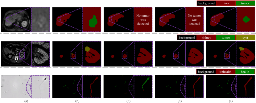
Figure 5: Examples of segmentation results in the ATLAS, KiTS23, and SpermHealth datasets in different rows for error analysis. Examples contain ultra-small objects (i.e., tumor, cyst, and sperm), small objects (i.e., kidney), and objects with $>$10% area ratio (i.e., liver). (a) Input image, (b) Ground truth, and prediction results of (c) HRNet, (d) TransNetR, and (e) SvAttn (ours).

However, SvANet maintains a growing trend without decline, demonstrating its effectiveness in recognizing retinal vasculatures, which is crucial for diagnosing blindness-causing diseases. Besides, in ISIC 2018 and KiTS23 datasets, SvANet and over half of other methods exhibit a mDice trend resembling an “L” shape, as depicted in Fig. 4be. Fewer ultra-small objects in these datasets introduce significant variability, likely contributing to this “L” trend. In the PolypGen, ATLAS, and TissueNet datasets, there is a consistent increase in mDice trends, as shown in Fig. 4cdf. Notably, no change is observed in TissueNet between the small and all object scales, as both categories contain identical medical images. Closer inspection of the Fig. 4d and Tab. II reveals that SvANet is the only method that achieved a “V” trend in the ATLAS dataset, with the best mDice of 89.79% for segmenting ultra-small compared to small and all sizes of livers and tumors, underscoring SvANet’s capability to effectively discriminate ultra-small medical objects. Additionally, SvANet consistently displays narrow error bars (shown as color bands) across three object scales, indicating its robustness in accurately recognizing medical objects.

IV-C Results for the Dataset for Only Ultra-small Objects

To further evaluate the performance of SvANet in distinguishing ultra-small medical objects, experiments were conducted on the SpermHealth dataset, which exclusively has sperms with an area ratio of less than 1%. As shown in Tab. III, SvANet secured top performance in sperm segmentation within the SpermHealth dataset, achieving 72.58% in mDice, 61.44% in mIoU, 13.06×10^-4 in MAE, 72.50% in sensitivity, and 72.51% F2 score. SvANet’s performance in sperm segmentation notably exceeded that of other models, surpassing them by up to 36.66% in mDice, 26.16% in mIoU, 36.76% in sensitivity, and 36.74% in F2 score. Besides, the performance metrics (mDice, mIoU, sensitivity, and F2 score) gained in the SpermHealth dataset are significantly lower than those observed in ISIC 2018, PolypGen, ATLAS, and KiTS23 for all tested models, with a gap of $>$10%, because all sperms have an area lower than 1%, presenting limited learnable features and posing more significant challenges for differentiation.

TABLE IV: Ablation study results in the SpermHealth dataset on the ultra-small category. The best results are underlined in bold.

Ablation settings
		Cross-scale
MCBottleneck	MCAttn	guidance	SvAttn	AssemFormer	mDice	Sensitivity	p-value
					71.10	70.08	-
✓					71.25	70.48	0.042
✓	✓				71.77	70.70	0.033
✓	✓	✓			72.18	71.33	0.019
✓	✓	✓	✓		72.42	71.84	0.013
✓	✓	✓	✓	✓	72.58	72.51	0.001

TABLE V: Comparison of MCAttn with other advanced attention methods. The best results are underlined in bold.

	# Parameters
Attention module	/Million	mDice	Sensitivity	p-value
-	-	71.81	70.37	-
SE [27]	2.77	71.19	71.39	0.048
CBAM [28]	0.70	70.98	69.96	0.041
CoorAttn [29]	0.10	71.43	70.14	0.049
MCAttn (ours)	2.77	72.58	72.51	0.022

IV-D Ablation Studies

IV-D1 Main Components Ablation

Ablation studies were conducted and discussed in this section to investigate the influence of each module of SvANet. The results of ablation studies for the MCBottleneck, MCAttn, cross-scale guidance, SvAttn, and AssemFormer modules are presented in Tab. IV. As indicated in the first and second columns of Tab. IV, the inclusion of MCBottleneck and MCAttn results in improvements of +0.15% & +0.52% mDice and +0.40% & +0.22% sensitivity, respectively, suggesting that both modules significantly contribute to enhancing the diagnosis and accuracy of positive cases. Furthermore, when equipped with cross-scale guidance and SvAttn, SvANet achieves an additional +0.41% & +0.24% in mDice and +0.53% & +0.51% in sensitivity. The ablation of AssemFormer leads to an increase of +0.16% in mDice and +0.67% in sensitivity. The p-value for mDice is below 0.05, confirming the result reliability. In summary, MCAttn and cross-scale guidance are critical modules for enhancing prediction accuracy, while AssemFormer and MCBottleneck are vital in improving the accuracy of positive diagnostics in medical object segmentation.

IV-D2 MCAttn vs. Other Advanced Attention Methods

To assess the impact of different attention mechanisms within the MCBottleneck, three advanced attention modules, including squeeze-excitation (SE), convolution block attention module (CBAM), and coordinate attention (CoorAttn), were utilized as the control group. According to the results shown in Tab. V, MCAttn achieved performance improvements of over +1.15% in mDice and +1.12% sensitivity compared to these alternatives. Notably, the control group’s attention methods resulted in reduced performance, with decreases of up to -0.83% in mDice and -0.41% in sensitivity, underscoring the superior efficacy of MCAttn in enhancing medical image segmentation within a bottleneck structure. The p-value for mDice is below 0.05, affirming the reliability of the result.

IV-E Negative Case Studies

Examples of visualization results for ultra-small and small medical objects using the top three performance methods, HRNet, TransNetR, and SvANet in the ATLAS, KiTS23, and SpermHealth dataset are presented in Fig. 5. As indicated by the first two rows in Fig. 5, it is possible to overlook overlapped medical objects, particularly the ultra-small ones. For example, both HRNet and TransNetR failed to identify an ultra-small tumor inside the liver and missed an ultra-small cyst at the edge of the kidney. Although HRNet and TransNetR identified the kidney with a complete boundary, they incorrectly emphasized holes that are not part of the kidney in the example image. However, SvANet accurately differentiated between organs and their infected regions. Besides, SvANet reflected the morphological details of the liver, hepatic tumor, kidney, and cyst in the example image, aligning closely with the ground truth annotations. The lower-right image in Fig. 5 shows that SvANet precisely located all sperms’ positions and effectively recognized the region of the broken-line tail of an abnormal sperm. Conversely, tested methods like HRNet struggled to distinguish the broken-line shape. Moreover, TransNetR misclassified an unhealthy sperm head as healthy, as indicated by a green subregion in Fig. 5d. These visualization results align with the findings discussed in Sec. IV-B and Sec. IV-C, suggesting that SvANet holds significant potential for application in general small medical object recognition across various medical imaging modalities.

V Conclusion

This paper introduces SvANet, a novel network to improve the segmentation of small medical objects, aiding in the detection of life-threatening diseases and supporting in vitro fertilization. The experimental outcomes demonstrate that the SvANet is highly effective in distinguishing medical objects of various sizes. SvANet consistently outperformed other SOTA methods, achieving 96.12%, 96.11%, 89.79%, 84.15%, 80.25%, 73.05%, and 72.58% in mDice for segmenting objects with less than 1% image area across multiple datasets, including KiTS23, ISIC 2018, ATLAS, PolypGen, TissueNet, FIVES, and SpermHealth. Additionally, the visualization results confirm that SvANet accurately identifies the locations and morphologies of all medical objects, demonstrating its exceptional capability in the segmentation of small medical objects. These findings underscore the potential of SvANet as a significant advancement in medical imaging.

Supplement

This section discusses auxiliary but noteworthy settings and circumstances related to this work. Additional experiments presented herein aim to clearly demonstrate the advancements offered by our models.

Area Computation

The same instance across different images is treated as an independent object because several datasets do not have instance labels during inference. For a fair comparison, each object instance is counted once per image. Area computation results indicate that 18% of retinal vasculatures in FIVES [1], 40% of skin lesions in ISIC 2018 [2], 63% of polyps in PolypGen [3], 74% of hepatic tumors and livers in ATLAS [6], 99% of kidneys and corresponding neopasms in KiTS23 [4], and 100% tissue cells in TissueNet [7]. The area calculation codes are publically available at https://github.com/anthonyweidai/circle_extractor.

Network Instantiation

The input medical image is initially processed through a stem module, which consists of a strided convolution that reduces the resolutions of the image by half. The output resolutions at the end of the five stages are 1/2, 1/4, 1/8, 1/16, and 1/32. The output channels of the bottom row blocks are 64, 64, 128, 256, and 512, respectively.

Inference Time

This section quantifies the inference characteristics of the tested networks, including the number of parameters (# Parameters), multiply-accumulate operations (MACs), and inferencing speed. The number of classes was set to eight, and other configurations were consistent with those described in Sec. IV-A2. The inference speed results, averaged over 1000 runs, are presented in Tab. VI. Tab. VI illustrates that SvANet achieved a real-time analysis of medical images with 46.91 frames per second (FPS), which is twice as fast as UNet and 19% faster than TransNetR. This performance level is suitable for self-examination and clinical diagnostic applications.

TABLE VI: Model size and inference time comparison.

	# Parameters	MACs	Speed
Methods	/Million	/Billion	/FPS
UNet (MICCAI’15) [9]	34.53	200.75	22.76
UNet++ (TMI’19) [10]	9.16	107.09	43.69
PraNet (MICCAI’20) [11]	30.34	25.65	68.16
HRNet (TPAMI’20) [25]	63.60	65.80	78.95
HSNet (CBM’22) [14]	37.17	25.09	71.40
CFANet (PR’23) [13]	25.71	115.63	60.89
TransNetR (MIDL’24) [21]	27.27	44.71	39.39
SvANet (Ours)	177.64	312.76	46.91

AssemFormer Module Understanding

To better understand AssemFormer’s capabilities, we visualized the feature maps generated by AssemFormer, as shown in Fig. 6. In Fig. 6, progressing from left to right, the AssemFormer increasingly highlights smaller areas that more accurately align with the ground truth, especially notable in scenarios with fewer medical objects. For instance, the first row of Fig. 2 demonstrates how the thin lines of retinal vasculature and light reflections are initially emphasized, becoming progressively thicker. Subsequently, these lines become shorter and more focused on a smaller region corresponding to the optic disc location, as depicted in the second first of Fig. 2ef. Large-scale distortions, such as noise or compression defects, play a role in this observed trend where the concentration of feature maps intensifies with a deeper layer. The pattern of increased feature map concentration is consistent across the segmentation of various medical objects, including skin lesions, polyps, hepatic tumors, livers, kidneys, tissue cells, and sperms.

The multi-head self-attention mechanism of AssemFormer, described in Eq. 7, facilitates patch interactions and enriches the context information. In contrast to Fig. 2, from left to right, the feature maps evolve from AssemFormer from coarse to fine representations. As illustrated in Fig. 2f, the AssemFormer enhances the visibility and precise localization of small medical objects such as glaucoma, nevus, polyp, hepatic tumor, kidney, tissue cell, and sperm, highlighting their morphological details and exact positions.

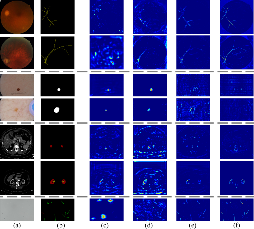
Figure 6: Visualization of output feature maps from AssemFormer. Columns (a) and (b) display the original images and their corresponding ground truth annotations, respectively. Columns (c), (d), and (f) illustrate the output feature maps from AssemFormer at stages 1, 2, 3, and 4 across seven benchmark datasets.

Robustness analysis

To quantify the robustness and adaptability of SvANet vs. other SOTA methods, receiver operating characteristic (ROC) curves of tested methods in the SpermHealth dataset are employed and illustrated in Fig. 7. The ROC curve of SvANet, represented by the red line in Fig. 7, blends nearest towards the top-left corner, with the highest area under the curve (AUC) of 0.9905, surpassing other SOTA methods by up to AUC of +0.0995. Besides, the ROC curve of HSNet is close to the lower-right corner and under all other curves, with the lowest AUC of 0.8910. The ROC and AUC results of HSNet are consistent with Tab. III, demonstrating that HSNet struggled to recognize sperms.

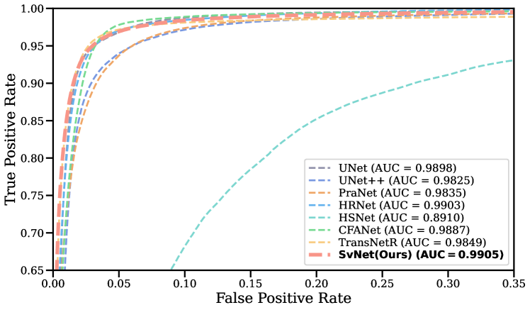
Figure 7: Receiver operating characteristic (ROC) curves for tested models in the SpermHealth dataset.

Full Negative Case Studies

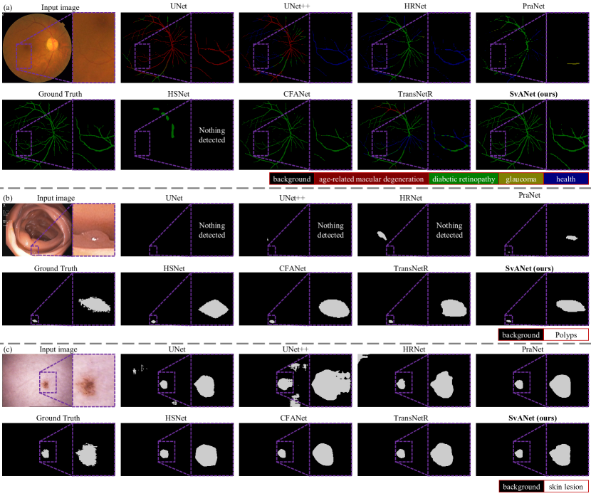
Figure 8: Examples of segmentation results for error analysis from the (a) FIVES, (b) PolypGen, and (c) ISIC 2018 datasets.

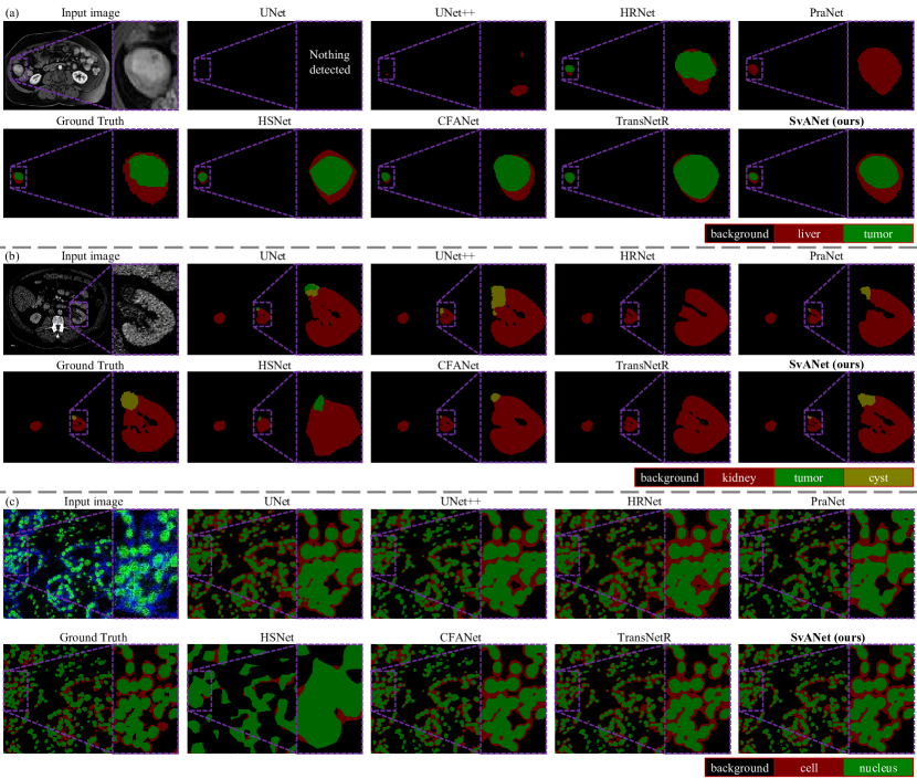
Figure 9: Examples of segmentation results for error analysis from the (a) ATLAS, (b) KiTS23, and (c) TissueNet datasets.

Examples of visualization results of small medical objects in the FIVES, PolypGen, ISIC 2018, ATLAS, KiTS23, and TissueNet datasets are presented in Fig. 8 and Fig. 9. As shown in Fig. 8a, UNet misclassified diabetic retinopathy (green region) as age-related macular degeneration (red region), UNet++, HRNet, & TransNetR misclassified diabetic retinopathy as health retinal vessels (blue region), and PraNet misclassified diabetic retinopathy as glaucoma (yellow region). Besides, HSNet could not detect retinal vasculature in the zoomed-in region. Moreover, none of SOTA methods in the control group can recover retinal vessels on the bottom of the zoomed-in region. Conversely, SvANet not only correctly classified diabetic retinopathy but also effectively detected the retinal vessels’ position and shape.

For the polyps diagnosis as presented in Fig. 8b, SOTA methods such as PraNet either detected a smaller polyp area than the ground truth, or other methods, including HSNet, CFANet, and TransNetR, regarded a larger region than the ground truth. Additionally, UNet, UNet++, and HRNet cannot detect the polyp in the example image. Besides, the detected regions from methods in the control group are far different from the ground truth. However, SvANet not only recognized an area close to the ground truth but also kept similar shapes as ground truth annotations. For the skin lesion examination illustrated in Fig. 8c, methods in the control group caught a larger region that covered the ground truth annotations, bringing the problem that the boundary of skin lesion was underrated. In contrast, SvANet distinguished a skin lesion of a similar size as the ground truth and uncovered its sawtooth-shaped boundary.

For the MRI and CT image modalities analysis, as shown in Fig. 9ab, it is possible to overlook the overlapped medical objects. For instance, UNet++ and PraNet did not discover a tumor in the liver, and HRNet and TransNetR missed a cyst at the edge of the kidney. Besides, UNet and HSNet wrongly recognized a cyst as a tumor. Although the organ region (e.g., liver and kidney) detected by SOTA methods in the control group could be complete, the illness regions, such as the tumor and cyst, were either larger than the ground truth (hepatic tumor) or smaller than the ground truth (cyst) in the example image. However, SvANet correctly sorted out organs and their infected regions. Moreover, SvANet reflected the morphology details of the liver, hepatic tumor, kidney, and cyst in the example image, which are similar to the ground truth annotations.

For tissue cell recognition in the TissueNet dataset, as shown in Fig. 9c, TransNetR and SvANet detailly divided cell boundaries, and they successfully labeled the cells and nuclei regions, as close as resembling the ground truth. In contrast, other SOTA methods struggled to categorize cells and nuclei, and these methods struggled to differentiate cell boundaries, resulting in merging several cells into one.

The visualization results demonstrate SvANet’s capability to differentiate small medical objects across multiple image modalities and object types, consistent with the quantitative results as Sec. IV-B. Thus, SvANet holds tremendous potential for application in the analysis of small medical objects for disease diagnostics, surgeries, etc.

Extracurricular Ablation

The configurations of training and testing are the same as that in Sec. IV-D unless specified.

Place of MCAttn

The ablation study presented in Tab. VII demonstrates that using MCAttn exclusively within MCBottleneck delivered at least +0.26% in mDice and +1.06% in sensitivity compared to its application in AssemFormer.

TABLE VII: Impact of the attention modules in MCBottleNeck and AssemFormer. Configurations include (0): None, (1): Squeeze-excitation, and (2) MCAttn. The best results are underlined in bold.

Attention of	Attention of AssemFormer
MCB*	inside MCB	outside MCB	mDice	Sensitivity
(0)	(0)	(0)	71.81	70.37
(1)	(1)	(1)	69.99	68.19
(2)	(2)	(2)	70.54	69.45
(2)	(1)	(2)	72.57	71.25
(2)	(0)	(2)	70.92	68.97
(2)	(0)	(1)	72.32	71.45
(2)	(0)	(0)	72.58	72.51
(2)	(1)	(0)	71.49	70.43
(2)	(2)	(0)	71.82	70.53
*MCB: MCBottleneck

The Number of Pooled Tensors for MCAttn

The selection of the size and number of pooled tensors for MCAttn is crucial for expanding network variants. We tested combinations (1, 2), (1, 2, 3), (2, 3), and (1, 2, 3, 4). The results, shown in the first, second, and fourth rows of Tab. VIII, reveal that the (1, 2, 3) combination of pooled tensors outperformed (1, 2) and (1, 2, 3, 4) combinations, with improvements exceeding 2.86% & 1.19% in mDice and 4.01% & 1.66%, respectively. Further analysis, as indicated in the second and third rows of Tab. VIII, highlights the necessity of a pool size of 1, leading to an increase of 0.82% in mDice and +2.27% in sensitivity. These findings emphasize the importance of maintaining an optimal level of variation in the network. An insufficient number of pooled tensors can limit performance, whereas an excessive number can introduce too much stochasticity. Thus, striking the right balance is critical for maximizing the effectivness of MCAttn within the model.

TABLE VIII: Size combinations of pooled feature maps in MCAttn (Unit: %). The best results are underlined in bold.

Pooled tensor sizes	mDice	Sensitivity
(1, 2)	69.72	68.50
(1, 2, 3)	72.58	72.51
(2, 3)	71.76	70.24
(1, 2, 3, 4)	71.39	70.85

Place of AssemFormer

Given that AssemFormer operates both inside and outside the MCBottleneck, it is essential to explore its impact in these settings. As indicated in Tab. IX, positioning AssemFormer only inside or outside MCBottleneck leads to reductions in performance, with drops ranging from 1.25% $\sim$ 1.30% in mDice and 1.60% $\sim$ 1.86% in sensitivity. Conversely, employing AssemFormer in both locations yields improvements of 0.16% in mDice and 0.67% in sensitivity, enhancing sperms diagnosis. Such results suggest the importance of consistent tensor operations before and after concatenation for cross-scale guidance, as depicted in Fig. 1, ensuring that tensors are processed in the same latent space.

TABLE IX: Impact of the AssemFormer module located inside and outside the MCBottleneck. The best results are underlined in bold.

AssemFormer
Inside MCB*	Outside MCB	mDice	Sensitivity
		72.42	71.84
✓		71.17	69.98
	✓	71.12	70.34
✓	✓	72.58	72.51
*MCB: MCBottleneck

Concatenation or Addition after MCBottleneck

As shown in Fig. 1, post-MCBottleneck concatenation operations can be replaced by using either direct links or addition operations. Nevertheless, the ablation results detailed in Tab. X demonstrate that concatenation for post-MCBottleneck is more effective. Specifically, concatenation delivered improvements of 3.42% & 1.43% in mDice and 6.07% & 3.12% in sensitivity, compared to direct links and addition operations, separately. The findings underscore the importance of preserving feature characteristics and depth information in outputs from the MCBottleneck and cross-scale guidance.

TABLE X: Comparison of concatenation versus addition operations after MCBottleneck. The best results are underlined in bold.

	# Parameters
Settings	/Million	mDice	Sensitivity
-	-	69.16	66.44
Addition	12.17	71.15	69.39
Cancatenation	38.41	72.58	72.51

References

- [1] K. Jin, X. Huang, J. Zhou, Y. Li, Y. Yan, Y. Sun, Q. Zhang, Y. Wang, and J. Ye, “FIVES: A fundus image dataset for artificial intelligence based vessel segmentation,” Scientific Data, vol. 9, no. 1, p. 475, 2022.
- [2] N. Codella, V. Rotemberg, P. Tschandl, M. E. Celebi, S. Dusza, D. Gutman, B. Helba, A. Kalloo, K. Liopyris, M. Marchetti et al., “Skin lesion analysis toward melanoma detection 2018: A challenge hosted by the international skin imaging collaboration (ISIC),” arXiv preprint arXiv:1902.03368, 2019.
- [3] S. Ali, D. Jha, N. Ghatwary, S. Realdon, R. Cannizzaro, O. E. Salem, D. Lamarque, C. Daul, M. A. Riegler, K. V. Anonsen et al., “A multi-centre polyp detection and segmentation dataset for generalisability assessment,” Scientific Data, vol. 10, no. 1, p. 75, 2023.
- [4] N. Heller, F. Isensee, D. Trofimova et al., “The KiTS21 challenge: Automatic segmentation of kidneys, renal tumors, and renal cysts in corticomedullary-phase CT,” 2023.
- [5] H. Sung, J. Ferlay, R. L. Siegel, M. Laversanne, I. Soerjomataram, A. Jemal, and F. Bray, “Global cancer statistics 2020: Globocan estimates of incidence and mortality worldwide for 36 cancers in 185 countries,” CA: A Cancer Journal for Clinicians, vol. 71, no. 3, pp. 209–249, 2021.
- [6] F. Quinton, R. Popoff, B. Presles, S. Leclerc, F. Meriaudeau, G. Nodari, O. Lopez, J. Pellegrinelli, O. Chevallier, D. Ginhac et al., “A tumour and liver automatic segmentation (ATLAS) dataset on contrast-enhanced magnetic resonance imaging for hepatocellular carcinoma,” Data, vol. 8, no. 5, p. 79, 2023.
- [7] N. F. Greenwald, G. Miller, E. Moen, A. Kong, A. Kagel, T. Dougherty, C. C. Fullaway, B. J. McIntosh, K. X. Leow, M. S. Schwartz et al., “Whole-cell segmentation of tissue images with human-level performance using large-scale data annotation and deep learning,” Nature Biotechnology, vol. 40, no. 4, pp. 555–565, 2022.
- [8] C. Dai, Z. Zhang, J. Huang, X. Wang, C. Ru, H. Pu, S. Xie, J. Zhang, S. Moskovtsev, C. Librach et al., “Automated non-invasive measurement of single sperm’s motility and morphology,” IEEE Transactions on Medical Imaging, vol. 37, no. 10, pp. 2257–2265, 2018.
- [9] O. Ronneberger, P. Fischer, and T. Brox, “U-Net: Convolutional networks for biomedical image segmentation,” in International Conference on Medical Image Computing and Computer Assisted Intervention. Springer, 2015, pp. 234–241.
- [10] Z. Zhou, M. M. R. Siddiquee, N. Tajbakhsh, and J. Liang, “UNet++: Redesigning skip connections to exploit multiscale features in image segmentation,” IEEE Transactions on Medical Imaging, vol. 39, no. 6, pp. 1856–1867, 2019.
- [11] D.-P. Fan, G.-P. Ji, T. Zhou, G. Chen, H. Fu, J. Shen, and L. Shao, “PraNet: Parallel reverse attention network for polyp segmentation,” in International Conference on Medical Image Computing and Computer Assisted Intervention. Springer, 2020, pp. 263–273.
- [12] A. Lou, S. Guan, and M. Loew, “CaraNet: Context axial reverse attention network for segmentation of small medical objects,” Journal of Medical Imaging, vol. 10, no. 1, p. 014005, 2023.
- [13] T. Zhou, Y. Zhou, K. He, C. Gong, J. Yang, H. Fu, and D. Shen, “Cross-level feature aggregation network for polyp segmentation,” Pattern Recognition, vol. 140, p. 109555, 2023.
- [14] W. Zhang, C. Fu, Y. Zheng, F. Zhang, Y. Zhao, and C.-W. Sham, “Hsnet: A hybrid semantic network for polyp segmentation,” Computers in Biology and Medicine, vol. 150, p. 106173, 2022.
- [15] X. Pan, J. Cheng, F. Hou, R. Lan, C. Lu, L. Li, Z. Feng, H. Wang, C. Liang, Z. Liu et al., “SMILE: Cost-sensitive multi-task learning for nuclear segmentation and classification with imbalanced annotations,” Medical Image Analysis, vol. 88, p. 102867, 2023.
- [16] W. Dai, R. Liu, T. Wu, M. Wang, J. Yin, and J. Liu, “Deeply supervised skin lesions diagnosis with stage and branch attention,” IEEE Journal of Biomedical and Health Informatics, vol. 28, no. 2, pp. 719–729, 2024.
- [17] J. Ding, N. Xue, G.-S. Xia, X. Bai, W. Yang, M. Y. Yang, S. Belongie, J. Luo, M. Datcu, M. Pelillo et al., “Object detection in aerial images: A large-scale benchmark and challenges,” IEEE Transactions on Pattern Analysis and Machine Intelligence, vol. 44, no. 11, pp. 7778–7796, 2021.
- [18] D. Guo, L. Zhu, Y. Lu, H. Yu, and S. Wang, “Small object sensitive segmentation of urban street scene with spatial adjacency between object classes,” IEEE Transactions on Image Processing, vol. 28, no. 6, pp. 2643–2653, 2018.
- [19] J. Miao, S.-P. Zhou, G.-Q. Zhou, K.-N. Wang, M. Yang, S. Zhou, and Y. Chen, “SC-SSL: Self-correcting collaborative and contrastive co-training model for semi-supervised medical image segmentation,” IEEE Transactions on Medical Imaging, 2023.
- [20] J. Long, E. Shelhamer, and T. Darrell, “Fully convolutional networks for semantic segmentation,” in Proceedings of the IEEE Conference on Computer Vision and Pattern Recognition, 2015, pp. 3431–3440.
- [21] D. Jha, N. K. Tomar, V. Sharma, and U. Bagci, “Transnetr: Transformer-based residual network for polyp segmentation with multi-center out-of-distribution testing,” in Medical Imaging with Deep Learning. PMLR, 2024, pp. 1372–1384.
- [22] L.-C. Chen, Y. Zhu, G. Papandreou, F. Schroff, and H. Adam, “Encoder-decoder with atrous separable convolution for semantic image segmentation,” in Proceedings of the European Conference on Computer Vision, 2018, pp. 801–818.
- [23] H. Zhao, J. Shi, X. Qi, X. Wang, and J. Jia, “Pyramid scene parsing network,” in Proceedings of the IEEE Conference on Computer Vision and Pattern Recognition, 2017, pp. 2881–2890.
- [24] Y. Mei, Y. Fan, Y. Zhang, J. Yu, Y. Zhou, D. Liu, Y. Fu, T. S. Huang, and H. Shi, “Pyramid attention network for image restoration,” International Journal of Computer Vision, vol. 131, no. 12, pp. 3207–3225, 2023.
- [25] J. Wang, K. Sun, T. Cheng, B. Jiang, C. Deng, Y. Zhao, D. Liu, Y. Mu, M. Tan, X. Wang et al., “Deep high-resolution representation learning for visual recognition,” IEEE Transactions on Pattern Analysis and Machine Intelligence, vol. 43, no. 10, pp. 3349–3364, 2020.
- [26] S. Sang, Y. Zhou, M. T. Islam, and L. Xing, “Small-object sensitive segmentation using across feature map attention,” IEEE Transactions on Pattern Analysis and Machine Intelligence, vol. 45, no. 5, pp. 6289–6306, 2022.
- [27] J. Hu, L. Shen, and G. Sun, “Squeeze-and-excitation networks,” in Proceedings of the IEEE Conference on Computer Vision and Pattern Recognition, 2018, pp. 7132–7141.
- [28] S. Woo, J. Park, J.-Y. Lee, and I. S. Kweon, “CBAM: Convolutional block attention module,” in Proceedings of the European Conference on Computer Vision, 2018, pp. 3–19.
- [29] Q. Hou, D. Zhou, and J. Feng, “Coordinate attention for efficient mobile network design,” in Proceedings of the IEEE/CVF Conference on Computer Vision and Pattern Recognition, 2021, pp. 13 713–13 722.
- [30] X. He, E.-L. Tan, H. Bi, X. Zhang, S. Zhao, and B. Lei, “Fully transformer network for skin lesion analysis,” Medical Image Analysis, vol. 77, p. 102357, 2022.
- [31] A. Dosovitskiy, L. Beyer, A. Kolesnikov, D. Weissenborn, X. Zhai, T. Unterthiner, M. Dehghani, M. Minderer, G. Heigold, S. Gelly et al., “An image is worth 16x16 words: Transformers for image recognition at scale,” in International Conference on Learning Representations, 2020.
- [32] F. Hörst, M. Rempe, L. Heine, C. Seibold, J. Keyl, G. Baldini, S. Ugurel, J. Siveke, B. Grünwald, J. Egger et al., “CellViT: Vision transformers for precise cell segmentation and classification,” Medical Image Analysis, vol. 94, p. 103143, 2024.
- [33] S. Mehta and M. Rastegari, “Mobilevit: Light-weight, general-purpose, and mobile-friendly vision transformer,” in International Conference on Learning Representations, 2021.
- [34] A. Vaswani, N. Shazeer, N. Parmar, J. Uszkoreit, L. Jones, A. N. Gomez, Ł. Kaiser, and I. Polosukhin, “Attention is all you need,” Advances in Neural Information Processing Systems, vol. 30, 2017.
- [35] I. Loshchilov and F. Hutter, “Decoupled weight decay regularization,” arXiv preprint:1711.05101, 2017.
- [36] Loshchilov, Ilya and Hutter, Frank, “SGDR: Stochastic gradient descent with warm restarts,” in International Conference on Learning Representations, 2016, pp. 1–16.