Split Conformal Prediction under Data Contamination

Abstract

Conformal prediction is a non-parametric technique for constructing prediction intervals or sets from arbitrary predictive models under the assumption that the data is exchangeable. It is popular as it comes with theoretical guarantees on the marginal coverage of the prediction sets and the split conformal prediction variant has a very low computational cost compared to model training. We study the robustness of split conformal prediction in a data contamination setting, where we assume a small fraction of the calibration scores are drawn from a different distribution than the bulk. We quantify the impact of the corrupted data on the coverage and efficiency of the constructed sets when evaluated on clean test points, and verify our results with numerical experiments. Moreover, we propose an adjustment in the classification setting which we call Contamination Robust Conformal Prediction, and verify the efficacy of our approach using both synthetic and real datasets.

1 Introduction

Conformal prediction for uncertainty quantification (Gammerman et al., 1998; Vovk et al., 2005) has seen a surge of popularity in recent years, with prominent applications in machine learning algorithms for regression and classification; see Balasubramanian et al. (2014) and Angelopoulos and Bates (2021). Recent applications include graph neural networks (for example Clarkson (2023); Zargarbashi et al. (2023)) and time series forecasting, see for example Stankeviciute et al. (2021). Conformal prediction is a family of algorithms that generate finite sample valid prediction intervals or sets from an arbitrary black-box machine learning model. Conformal prediction may be thought of as a wrapper around a fitted model that uses a set of exchangeable held-out data to calibrate prediction sets. The possibly most wide-spread method, split-conformal (explained in more detail in Section 2), also requires trivial computational overhead when compared to model fitting.

One aspect that has not received much attention to date is applying conformal prediction to data containing outliers. Although conformal prediction yields intervals with finite sample guarantees when the model is correctly specified, if outliers are not corrected, the conformal prediction intervals may not provide the coverage that the user expects. This paper addresses this issue. Our setting is that of a Huber-type mixture model (Huber (1964, 1965)) of independent observations which are assumed to come from a distribution $\pi_{1}$, but are actually contaminated by a small number of observations which have distribution $\pi_{2}$. An observation from $\pi_{1}$ is called clean. A typical research question is then to predict the clean response, see for example Chen et al. (2022) ; more background on robust statistics can be found for example in Huber and Ronchetti (2011).

Intuitively, if one knew which component of the mixture each data point was sampled from, one could simply calibrate the prediction set using only samples from the same mixture as the test point as these data points are exchangeable. We instead assume that it is unknown which data points are clean, and study the impact of contamination on the coverage and width of the constructed sets. In particular, we provide lower and upper bounds on the coverage under the assumption that the new data point is clean. We provide a general robustness result regarding the construction of conformal prediction sets. Under the additional assumption that the contaminating distribution stochastically dominates the clean distribution, as may be the case in a regression setting, we derive an over-coverage guarantee, and we give a companion result for the situation that the clean distribution stochastically dominates the contaminating distribution.

Moreover, in a classification setting, we devise a remedy for adjusting the prediction sets to obtain improved coverage guarantees. We call this method Contamination Robust Conformal Prediction, abbreviated CRCP. Both on synthetic data and on a benchmark data containing real-world label noise, namely the CIFAR-10N data set by Wei et al. (2022), we find that while standard conformal prediction can give considerable over-coverage, CRCP not only ameliorates this issue but also produces considerably narrower prediction intervals.

The paper is structured as follows. Section 2 gives background on split conformal prediction under the assumption that the calibration and the test data are exchangeable. In Section 3, split conformal prediction under data contamination is introduced; it gives theoretical results for coverage and robustness, and refined results under stochastic dominance assumptions. In Section 4, CRCP as a remedy for adjusting over-coverage in a classification setting is devised. Experiments are shown in Section 5, with Subsection 5.1 illustrating CRCP on synthetic datasets and Subsection 5.2 comparing CRCP and standard conformal prediction on the CIFAR-10N dataset from Wei et al. (2022). A detailed discussion of related results, which draws on results which are derived in this paper, is postponed to the concluding Section 6. A technical proof as well as experimental details are found in the Appendix. The code to reproduce the results presented in this paper is available at https://github.com/jase-clarkson/cp_under_data_contamination.

2 Split Conformal Prediction for Exchangeable Data

Here we lay out notation and briefly describe the split conformal prediction procedure in the exchangeable setting; see Angelopoulos and Bates (2021) for an excellent extensive introduction. Suppose we have access to a pre-fitted model $\hat{f}:\mathcal{X}\rightarrow\mathcal{Y}$, and a set of calibration data points $Z_{i}=(X_{i},Y_{i})$, $i=1,\dots,n$ that were not used to fit the model. The goal is to construct a $(1-\alpha)$-probability prediction set for a test datapoint $Z_{n+1}=(X_{n+1},Y_{n+1})$, where $\alpha$ is a user-specified desired level of coverage. Conformal prediction uses a score function $S:\mathcal{X}\times\mathcal{Y}\rightarrow\mathbb{R}$, which measures the agreement between the model predictions and the targets. We assume without loss of generality that the score function is negatively oriented; a smaller score indicates a better fit. In this sense the score function is essentially a loss function. The pre-fitted model is only needed to obtain the scores; once the scores are available, the pre-fitted model no longer plays any role.

The split conformal prediction procedure proceeds as follows; one first computes the score for each calibration data-point $S_{i}=S(X_{i},Y_{i})$. For a desired coverage of at least $1-\alpha$, the crucial step is to then estimate the prediction set boundary $\hat{q}$ as

$$\hat{q}=Q_{1-\alpha}\left(\sum_{i=1}^{n}\delta_{S_{i}}+\delta_{+\infty}\right),$$ (1)

where for a probability measure $\mu$ on $\mathbb{R}$, $Q_{1-\alpha}(\mu)=\inf\{x:\mu((-\infty,x])\geq 1-\alpha\}$; here $\delta_{x}$ is the delta-measure, representing point mass at $x$. The quantity $\hat{q}$ in (1) can be seen as an empirical $p$-value; the procedure is equivalent to taking the $i$th order statistic of the scores $\{S_{1},\ldots,S_{n}\}$, given by $\hat{q}=S_{(i)}$, where $i=\lceil(1-\alpha)(n+1)\rceil$ (ties are broken at random by adding a small independent uniform random variable). Here we recall that the order statistics of $S_{1},\ldots,S_{n}$ are $S_{(1)}\leq S_{(2)}\leq\cdots\leq S_{(n)}$. Finally, a prediction set is constructed as

$$\widehat{C}_{n}\left(X_{n+1}\right)=\left\{y\in\mathcal{Y}:S\left(X_{n+1},y\right)\leq\hat{q}\right\}.$$ (2)

If the calibration and test data are exchangeable, then we have the coverage guarantee

$$1-\alpha\leq\mathbb{P}\left(Y_{n+1}\in\widehat{C}_{n}\left(X_{n+1}\right)\right)\leq 1-\alpha+\frac{1}{n+1}.$$ (3)

Here the probability is taken over all data $(X_{i},Y_{i}),i=1,\ldots,n+1$. It is important to note that the coverage guarantee provided by conformal prediction is only marginal; for example, if $T_{n+1}$ is a random quantity such that $X_{n+1}$ and $T_{n+1}$ are dependent, then the coverage guarantee (3) does not include a guarantee for $\mathbb{P}\left(Y_{n+1}\in\widehat{C}_{n}\left(X_{n+1}\right)|{T}_{n+1}=x\right).$ We will revisit this point in the following section when discussing data contamination.

3 Split Conformal Prediction under Data Contamination

A standard model for data contamination is the Huber $\epsilon$-contamination model (Huber, 1964, 1965), as follows. Let $\epsilon\in[0,1)$. Suppose that the calibration data are sampled i.i.d from a mixture model

$$Z_{i}=(X_{i},Y_{i})\sim(1-\epsilon)\pi_{1}+\epsilon\pi_{2},$$ (4)

where $\pi_{1},\pi_{2}$ are two distribution functions over $\mathcal{X}\times\mathcal{Y}$. This model can be interpreted as a small fraction $\epsilon$ of the scores being outliers with a different distribution from the bulk. Under this model, the scores $S(X_{i},Y_{i})$ of the data are also distributed as a mixture, $S_{i}=S(X_{i},Y_{i})\sim\tilde{{\Pi}},$ where $\tilde{\Pi}$ has cumulative distribution function (cdf ) $\tilde{F}=(1-\epsilon)F_{1}+\epsilon F_{2}$ with $F_{1},F_{2}$ cumulative distribution functions over the scores computed from each mixture component. We let ${\Pi}_{j}$ denote the distribution of the scores $S(X_{i},Y_{\color[rgb]{0,0,0}i})$ when $(X_{i},Y_{i})\sim\pi_{j}$, for $j=1,2$. In this setup, the contamination occurs independently of the previous observations.

We denote the quantile in Equation (1) estimated over the corrupted calibration data as $\tilde{q}$. By de Finetti’s Theorem, mixture models are exchangeable and so conformal prediction provides coverage on future test points; however this coverage is marginal, and in particular only holds for future test points sampled from the contaminated mixture distribution so that we only have $\mathbb{P}(\tilde{S}_{n+1}\leq\tilde{q})\geq 1-\alpha$ for $\tilde{S}_{n+1}\sim\tilde{\Pi}$. In this paper, we are interested in the setting where the test point is assumed to be “clean”, i.e. that $S_{n+1}\sim\Pi_{1}$. We shall provide bounds on the coverage over future clean test points

$$\mathbb{P}\left(Y_{n+1}\in\widehat{C}_{n}\left(X_{n+1}\right)|Z_{n+1}\sim\pi_{1}\right)=\mathbb{P}\left(S_{n+1}\leq\tilde{q}|S_{n+1}\sim{\Pi_{1}}\right)=:\mathbb{P}_{1}(S_{n+1}\leq\tilde{q}).$$ (5)

Here $\mathbb{P}_{1}\neq P_{1}$ is an abbreviation for the probability which takes the randomness in $\tilde{q}$ into account but conditions on the observation $S_{n+1}$ being clean. As the random quantile $\tilde{q}$ was estimated using contaminated data, the coverage guarantee given in Equation (3) no longer holds.

We provide bounds on the coverage obtained under the corruption model (4). We then study the average change in prediction set size as a result of data contamination, and provide some remarks on when one might expect over- or under-coverage, illustrated by a regression example. The last part of this section studies classification under label noise.

Our results employ the following distances. For two distributions $Q_{1}$ and $Q_{2}$ on $\mathbb{R}$ with cdf’s $G_{1}$ and $G_{2}$ the Kolmogorov-Smirnov distance between $Q_{1}$ and $Q_{2}$ is

$$d_{KS}(Q_{1},Q_{2})=\sup_{x}|G_{1}(x)-G_{2}(x)|.$$ (6)

With $G_{1}$ and $G_{2}$ having inverses $G_{1}^{-1}$ and $G_{2}^{-1}$, the Wasserstein-$p$ distance between $Q_{1}$ and $Q_{2}$ is

$$W_{p}(Q_{1},Q_{2})=\left(\int_{0}^{1}|G_{1}^{-1}(q)-G_{2}^{-1}(q)|^{p}dq\right)^{\frac{1}{p}}\mbox{ and }W_{1}(Q_{1},Q_{2})=\int_{0}^{1}|G_{1}(q)-G_{2}(q)|dq.$$ (7)

3.1 Coverage

Lemma 3.1 captures the intuition that the difference in coverage increases with the contamination fraction $\epsilon$ and the magnitude of the contaminations, measured by $d_{KS}(F_{1},F_{2})$.

Lemma 3.1.

Under the mixture model, (4) when $(X_{n+1},Y_{n+1})\sim\pi_{1}$, we have

$$(1-\alpha)-\epsilon\,{{\mathbb{E}}}[F_{2}(\tilde{q})-F_{1}(\tilde{q})]\leq\mathbb{P}_{1}\left(Y_{n+1}\in\widehat{C}_{n}(X_{n+1})\right)\leq(1-\alpha)+\frac{1}{n+1}+\epsilon\,{{\mathbb{E}}}[F_{1}(\tilde{q})-F_{2}(\tilde{q})]$$ (8)

and $(1-\alpha)-\epsilon\,d_{KS}(\Pi_{1},\Pi_{2})\leq\mathbb{P}_{1}\left(Y_{n+1}\in\widehat{C}_{n}(X_{n+1})\right)\leq(1-\alpha)+\frac{1}{n+1}+\epsilon\,d_{KS}(\Pi_{1},\Pi_{2}).$

Proof 3.2.

Let $\tilde{S}_{n+1}$ be sampled from the mixture distribution $\tilde{S}_{n+1}\sim\tilde{P}$. We first derive the claimed lower bounds. By the lower bound given in Equation (3) applied to the mixed data, we have

$$\mathbb{P}(\tilde{S}_{n+1}\leq\tilde{q})\geq 1-\alpha.$$ (9)

Let $P$ be the distribution of the random quantity $\tilde{q}$. Then conditioning yields

$$\mathbb{P}(\tilde{S}_{n+1}\leq\tilde{q}) =\int_{\mathbb{R}}\mathbb{P}(\tilde{S}_{n+1}\leq\tilde{q}|\tilde{q}=q)dP(q)=\int_{\mathbb{R}}\{(1-\epsilon)F_{1}(q)+\epsilon F_{2}(q)\}dP(q),$$ (10)

where the last step in (10) follows from the independence of $S_{n+1}$ and $(S_{1},\ldots,S_{n})$. Substituting (10) into (9) and re-arranging gives $\int_{\mathbb{R}}F_{1}(q)dP(q)\geq(1-\alpha)-\epsilon\int_{\mathbb{R}}\{F_{2}(q)-F_{1}(q)\}dP(q)$. Finally, un-doing the conditioning gives

$$\int_{\mathbb{R}}F_{1}(q)dP(q)=\int_{\mathbb{R}}\mathbb{P}(S_{n+1}\leq q)dP(q) =\int_{\mathbb{R}}\mathbb{P}(S_{n+1}\leq\tilde{q}|\tilde{q}=q)dP(q)=\mathbb{P}_{1}(S_{n+1}\leq\tilde{q}),$$

with $\mathbb{P}_{1}$ as in Equation (5), proving the lower bound in (8). The lower bound in Kolmogorov-Smirnov distance follows directly from (6) applied to the lower bound in the inequality (8). The upper bounds are proved in an analogous fashion, applied to the upper bound in (3).

3.2 Robustness

Next we compare the expected size of prediction sets constructed using a clean calibration set drawn from $F_{1}$, and a corrupted sample drawn from the mixture. Here we exploit that $\tilde{q}$ is a random quantile which can be analysed using tools from order statistics. Suppose that $S_{1},\dots,S_{n}$ are i.i.d. absolutely continuous random variables with distribution function $F$ and density $f$. Let $S_{(i)}$ be the $i^{th}$ order statistic of this sample. Then, using Arnold et al. (2008), p.108,

$$\mathbb{E}[S_{(i)}]=\frac{1}{B(i,n-i+1)}\int_{\mathbb{R}}x(F(x))^{i-1}(1-F(x))^{n-i}f(x)dx,$$ (11)

where $B(\alpha,\beta)=\frac{\Gamma(\alpha)\Gamma(\beta)}{\Gamma(\alpha+\beta)}$ is the beta function. Moreover, $F(S_{(i)})=:U_{(i)}$ is beta distributed with pdf

$$\frac{1}{B(i,n-i+1)}x^{i-1}(1-x)^{n-i}.$$ (12)

In the following Lemma, we use the model (4) and the Wasserstein-$p$ distance $W_{p}$ from (7).

Lemma 3.3.

Let $S_{1},\dots,S_{n}$ be conformal scores sampled i.i.d. from ${\Pi_{1}}$, and let $\tilde{S}_{1},\dots,\tilde{S}_{n}$ be sampled i.i.d. from ${\tilde{\Pi}}$. We assume that these scores are absolutely continuous random variables. Define $i=\lceil(1-\alpha)(n+1)\rceil$ and let $S_{(i)},\tilde{S}_{(i)}$ be the $i^{th}$ order statistics of the first and second samples respectively. Then for any $p,q$ such that $\frac{1}{p}+\frac{1}{q}=1$, we have

$$\left|\mathbb{E}[\tilde{S}_{(i)}]-\mathbb{E}[S_{(i)}]\right|\leq C(n,i)W_{q}({\tilde{\Pi},\Pi_{1}}),$$ (13)

where $C(n,i)=\sup_{t\in[0,1]}\frac{t^{i-1}(1-t)^{n-i}}{B(i,n-i+1)}=\frac{1}{B(i,n-i+1)}\left(\frac{i-1}{n-1}\right)^{i-1}\left(\frac{n-i}{n-1}\right)^{n-i}.$ In particular, when $p=\infty$, $q=1$ we have that $\left|\mathbb{E}[\tilde{S}_{(i)}]-\mathbb{E}[S_{(i)}]\right|\leq\epsilon C(n,i)W_{1}({\Pi_{1},\Pi_{2}}).$

Proof 3.4.

Making the substitution $x=F^{-1}(u)$ in (11) and employing (12) we have

$$\mathbb{E}[S_{(i)}]=\int^{1}_{0}F^{-1}(u)\frac{u^{i-1}(1-u)^{n-i}}{B(i,n-i+1)}du\quad\text{ and }\quad\mathbb{E}[\tilde{S}_{(i)}]=\int^{1}_{0}\tilde{F}^{-1}(u)\frac{u^{i-1}(1-u)^{n-i}}{B(i,n-i+1)}du.$$

Therefore the expected difference between the corrupted and clean order statistics is

$$\left|\mathbb{E}[\tilde{S}_{(i)}]-\mathbb{E}[S_{(i)}]\right| \leq\int_{0}^{1}\left|(\tilde{F}^{-1}(u)-F_{1}^{-1}(u))\frac{u^{i-1}(1-u)^{n-i}}{B(i,n-i+1)}\right|du$$

$$\leq{(C(n,i)^{p})}^{\frac{1}{p}}\left(\int_{0}^{1}\left(\tilde{F}^{-1}(u)-F_{1}^{-1}(u)\right)^{q}du\right)^{\frac{1}{q}}=C(n,i)W_{q}({\tilde{\Pi},\Pi_{1}})$$ (14)

where the inequality in (14) follows from Hölder’s inequality. If $p=\infty$, $q=1$ then, using (7), we have $W_{1}({\tilde{\Pi},\Pi_{1}})={\int_{0}^{1}|\tilde{F}(x)-F_{1}(x)|dx}=\epsilon\,W_{1}({\Pi_{1},\Pi_{2}}).$

Lemma 3.3 thus gives a quantitative version of the intuition that when the mixture distributions are close, then so will be the quantiles of their scores. It is these quantiles which are used to obtain prediction intervals; if the quantiles are close then their corresponding prediction intervals will be close as well. In this sense Lemma 3.3 gives a robustness guarantee.

The assumption in Lemma 3.3 that the scores are absolutely continuous is mild; as ties are broken at random when they exist by adding a small random variable having a continuous uniform distribution which renders the thus adjusted scores to be absolutely continuous while retaining exchangeability.

3.3 Theoretical Guarantees under Stochastic Dominance

In the previous subsection we derived bounds on the coverage and robustness of the prediction sets constructed using contaminated data. We now introduce some conditions under which the Huber model (4) will always lead to over-(or under-)coverage under $S_{n+1}\sim\Pi_{1}$. In the following we will use a notion of stochastic ordering between random variables known as first-order stochastic dominance. For two real-valued variables $X_{1}\sim{\Pi_{1}},X_{2}\sim{\Pi_{2}}$, with corresponding cdf ’s $F_{1}$ and $F_{2}$, we say $X_{2}$ first order stochastically dominates $X_{1}$ if $1-F_{1}(x)\leq 1-F_{2}(x)\text{ for all }x\in{{\mathbb{R}}}.$ In particular, we then have $F_{1}(x)\geq F_{2}(x)$ for all $x\in\mathbb{R}$. We write ${\Pi_{1}}\leq_{s.d}{\Pi_{2}}$ to denote that $X_{2}\sim{\Pi_{2}}$ first order stochastically dominantes $X_{1}\sim{\Pi_{1}}$.

Over-coverage

The lower bound in (8) shows that if $\Pi_{1}\leq_{s.d}\Pi_{2}$ , then ${{\mathbb{E}}}[F_{2}(\tilde{q})-F_{1}(\tilde{q})]\leq 0$ and

$${{\mathbb{P}}}_{1}(S_{n+1}\leq\tilde{q})\geq 1-\alpha-\epsilon\,{{\mathbb{E}}}[F_{2}(\tilde{q})-F_{1}(\tilde{q})]\geq 1-\alpha.$$

In this case, conformal prediction still provides (conservative) coverage, but prediction set sizes may be inflated. We note that if $\Pi_{1}\leq_{s.d}\Pi_{2}$ then we also have that $\Pi_{1}\leq_{s.d}\tilde{\Pi}$, as

$$\tilde{F}(x)\leq F_{1}(x) \iff(1-\epsilon)F_{1}(x)+\epsilon F_{2}(x)\leq F_{1}(x)\iff F_{2}(x)\leq F_{1}(x).$$ (15)

Under-Coverage

If instead the contaminating distribution $\Pi_{2}$ stochastically dominates the clean distribution $\Pi_{1}$, Inequality (8) in Lemma 3.1 implies that for a $1-\alpha$ upper coverage bound we need a slightly stronger condition than $\Pi_{2}\leq_{s.d}\Pi_{1}$, namely that

$$F_{1}(x)-F_{2}(x)\leq-\frac{1}{\epsilon(n+1)}\quad\text{for all }x\in{{\mathbb{R}}}.$$ (16)

In this case by (8) we have

$${{\mathbb{P}}}_{1}(S_{n+1}\leq\tilde{q}) \leq(1-\alpha)+\frac{1}{n+1}+\epsilon\,{{\mathbb{E}}}[F_{2}(\tilde{q})-F_{1}(\tilde{q})]\leq(1-\alpha)+\frac{1}{n+1}-\frac{\epsilon}{\epsilon(n+1)}=1-\alpha.$$

Example 3.5 (A Regression Example).

Consider the regression model

$$Y =f(X)+E,\text{ with }E\sim(1-\epsilon)\,\mathcal{N}(0,\sigma_{1}^{2})+\epsilon\,\mathcal{N}(0,\sigma_{2}^{2}),$$ (17)

where $\mathcal{N}(\mu,\sigma^{2})$ denotes a normally distribution random variable with mean $\mu$ and variance $\sigma^{2}$, and $f:\mathcal{X}\rightarrow{{\mathbb{R}}}$ is a measurable regression function. Assume that a forecaster has access to the oracle model, i.e. $\hat{f}=f$, and uses the absolute residual score function $S(X,Y)=|Y-\hat{f}(X)|$. Then the scores from each mixture component are distributed as a half normal distribution, which has cdf

$$F_{i}(x)=\operatorname{erf}\left(\frac{x}{\sqrt{2}\sigma_{i}}\right),\quad x\geq 0$$ (18)

for $i=1,2$. The error function $\operatorname{erf}$ is increasing and so the clean distribution dominates the mixture (and hence coverage is maintained) if $\sigma_{1}\leq\sigma_{2}$.

Although one may expect that $\sigma_{1}>\sigma_{2}$ would imply under-coverage, this is not the case. In particular, if $\sigma_{1}>\sigma_{2}$, then for $x>0$,

$$F_{1}(x)-F_{2}(x) =\frac{2}{\pi}\int^{\frac{x}{\sqrt{2}\sigma_{1}}}_{\frac{x}{\sqrt{2}\sigma_{2}}}e^{-t^{2}}dt\leq-\frac{2}{\pi}e^{-\frac{x^{2}}{2\sigma_{1}^{2}}}\frac{x}{\sqrt{2}}\left(\frac{1}{\sigma_{2}}-\frac{1}{\sigma_{1}}\right)=-\frac{\sqrt{2}x}{\pi}\left(\frac{1}{\sigma_{2}}-\frac{1}{\sigma_{1}}\right){e^{-\frac{x^{2}}{2\sigma_{1}^{2}}}}.$$

By comparing this with (16) we find that for undercoverage we require that for all $x\geq 0$,

$$\frac{\sqrt{2}x}{\pi}\left(\frac{1}{\sigma_{2}}-\frac{1}{\sigma_{1}}\right){e^{-\frac{x^{2}}{2\sigma_{1}^{2}}}}\geq\frac{1}{\epsilon(n+1)}.$$ (19)

As $x>0$ can be chosen to violate this inequality, we thus see that $\sigma_{1}>\sigma_{2}$ is not sufficient for to guarantee under-coverage.

To demonstrate the sensitivity of coverage to the noise parameters $\sigma_{2}$ and $\epsilon$ we perform the following experiment using the model (17) with $f(X)=\beta^{T}X$ and $\sigma_{1}=1$, while varying $\epsilon$ and $\sigma_{2}$. For the experiment we choose the parameter vector $\beta\in{{\mathbb{R}}}^{p}$ as a standard multivariate Gaussian vector and keep this $\beta$ fixed. For each choice of $\sigma_{2}$ and $\epsilon$, we draw 1000 samples from this model for training and test. We fit a linear regression model on the training set and use the fitted model to calibrate conformal prediction with the absolute residual score function. We then draw 1000 clean samples for testing (i.e. with $\epsilon=0$ in (17)), construct prediction sets for each point and record the mean coverage. We repeat this experiment 100 times for a range of choices of $\epsilon$ and $\sigma_{2}$ and plot the mean and standard deviation of the coverage over these repetitions in Figure 1. In the left panel we see the transition between over- and under-coverage around $\sigma_{1}=\sigma_{2}=1.0$.

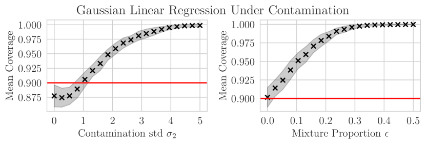
Figure 1: The mean and standard deviation of the coverage obtained over 100 repetitions of the regression experiment while varying $\epsilon$ and $\sigma_{2}$. The mean coverage is marked by crosses, and shaded regions show one standard deviation of the coverage. The straight line (in red) indicates the desired coverage level $0.9$. In the left panel we vary the standard deviation of the corruption $\sigma_{2}$ from 0 to 5, keeping $\epsilon=0.2$. In the right panel we vary the mixing proportion $\epsilon$ from $0$ to $0.5$, keeping $\sigma_{2}=3.0$.

Discussion

We note that the condition for over-coverage given in Equation (15) is weaker than the condition for under-coverage given in Equation (18); over-coverage requires only that $\Pi_{1}\leq_{s.d}\Pi_{2}$, whereas under-coverage requires a stronger condition where a margin of dominance is needed that depends on both the sample size and the mixture proportion. This finding suggests that conformal prediction possesses some inbuilt robustness to large outliers, in that it will continue to provide coverage (albeit with inflated prediction set sizes) for any level of corruption, but there is no such guarantee when the outliers are small.

In contrast to regression problems, in classification problems there is no natural ordering which could give rise to stochastic dominance arguments. In the next subsection we cover a model for classification under label noise in detail.

3.4 Classification under Label Noise

Suppose now the prediction set is constructed for a classification problem such that the targets take a discrete set of values $\mathcal{Y}=[K]$, where $[K]=\{1,\dots,K\}$. We write the generative model for the calibration data as $X_{i}\sim F_{X}$, and $Y_{i}\sim F_{Y|X}$, and assume that labels are corrupted with probability $\epsilon\in(0,\frac{1}{2})$, independently of the conditional distribution $X|Y$; we denote a sample from the corrupting distribution as ${Y}_{i}^{c}$. Then the observed class label $\tilde{Y}$ equals a draw $Y_{i}$ from $F_{Y|X}$ with probability $1-\epsilon$, and $\tilde{Y}_{i}$ equals a draw ${Y_{i}}^{c}$ from the corrupting distribution with probability $\epsilon$. It is possible that by chance the random draw $Y_{i}$ would take on the same value as the random draw ${Y_{i}}^{c}$. Let $P_{i}=\Pi_{1}(i)={{\mathbb{P}}}(Y=i),$ and $\tilde{P}_{i}=\tilde{P}_{i}(\epsilon)=\tilde{\Pi}(i)={{\mathbb{P}}}(\tilde{Y}=i),$ for $i\in[K]$, be the marginal label probabilities. Let $P\in{{\mathbb{R}}}^{K\times K}$ be the matrix with entries $P_{ji}=P_{ji}(\epsilon)={{\mathbb{P}}}(Y=j|\tilde{Y}=i)$ for $i,j\in[K]$; we assume that $P$ is invertible. Similarly we set $\tilde{P}_{ij}=\tilde{P}_{ij}(\epsilon)={{\mathbb{P}}}(\tilde{Y}=i|Y=j)$ so that by Bayes’ rule,

$$\tilde{P}_{i}P_{ji}=\tilde{P}_{ij}P_{j}.$$ (20)

In what follows we suppress the argument $\epsilon$ for easier notation. Finally, we define

$$F_{1}(q;i,j) ={{\mathbb{P}}}(S(X,i)\leq q|Y=j)\text{ and }\tilde{F}(q;i,j)={{\mathbb{P}}}(S(X,i)\leq q|\tilde{Y}=j)$$

for $q\in{{\mathbb{R}}}$, $i,j\in[K]$ as the cdfs of the conditional distribution of the score assigned to label $i$ given that the true or observed noisy label is equal to $j$. Then we have the following result.

Proposition 3.6.

Suppose that

$$\max_{c:c\neq i}\,{{\mathbb{P}}}(S(X,c)\leq q|Y=i)\leq{{\mathbb{P}}}(S(X,i)\leq q|Y=i)\text{ for all }q\in{{\mathbb{R}}},\;i\in[K].$$ (21)

Then ${{\mathbb{P}}}_{1}(Y_{n+1}\in\widehat{C}_{n}(X_{n+1)})\geq 1-\alpha.$

Condition (21) is natural; for $\epsilon=0$ then (21) is satisfied if $S(x,c)\geq S(x,i)$ when $i$ is the true label for $x$ and $c$ is any other label. This is guaranteed through assuming that the score is negatively oriented.

Proof 3.7.

In view of Lemma 3.1 it suffices to show that ${{\mathbb{E}}}[F_{2}(\tilde{q})-F_{1}(\tilde{q})]{\geq}0.$ Now,

$$F_{1}(q)=\sum_{i}P_{i}{{\mathbb{P}}}(S(X,i)\leq q|Y=i)=\sum_{i=1}^{K}P_{i}F_{1}(q,i,i)$$

and similarly $\tilde{F}(q)=\sum_{i}\tilde{P}_{i}{{\mathbb{P}}}(S(X,i)\leq q|\tilde{Y}=i)=\sum_{i=1}^{K}\tilde{P}_{i}\tilde{F}(q,i,i).$ Moreover as we assume ${Y}^{c}\perp X|Y$, given $Y=j$, knowing ${Y}^{c}$ does not contain any additional information on $S(X,i)$ and hence we have ${{\mathbb{P}}}(S(X,i)\leq q\,|\,\tilde{Y}=i,Y=j)={{\mathbb{P}}}(S(X,i)\leq q|Y=j),$ giving

$$\tilde{F}(q,i,i)=\sum_{j=1}^{K}{{\mathbb{P}}}(Y=j|\tilde{Y}=i){{\mathbb{P}}}(S(X,i)\leq q\,|\,\tilde{Y}=i,Y=j)=\sum_{j=1}^{K}P_{ji}F_{1}(q,i,j).$$ (22)

and, using (20), we obtain $\tilde{P}_{i}\tilde{F}(q,i,i)=\sum_{j=1}^{K}{P}_{j}\tilde{P}_{ij}F_{1}(q;i,j).$ Thus, we have

$$F_{1}(q)-\tilde{F}(q) =\sum_{i=1}^{K}\left(P_{i}F_{1}(q;i,i)-\tilde{P}_{i}\tilde{F}(q;i,i)\right)$$

$$=\sum_{i=1}^{K}P_{i}F_{1}(q;i,i)-\sum_{j=1}^{K}\left(P_{j}\tilde{P}_{jj}F_{1}(q;j,j)+\sum_{{i:}i\neq j}P_{j}\tilde{P}_{ij}F_{1}(q;i,j)\right)$$

$$=\sum_{i=1}^{K}P_{i}(1-\tilde{P}_{ii})F_{1}(q;i,i)-\sum_{j=1}^{K}\sum_{i:i\neq j}P_{j}\tilde{P}_{ij}F_{1}(q;i,j).$$

As $\sum_{i:i\neq j}\tilde{P}_{ij}=1-\tilde{P}_{jj}$ it follows that $F_{1}(q)-\tilde{F}(q)\geq\sum_{i=1}^{K}P_{i}(1-\tilde{P}_{ii})\left(F_{1}(q;i,i)-\max_{{c:}c\neq i}F_{1}(q;c,i))\right)$ which is $\geq 0$ due to Assumption (21).

As we assume that the score function is negatively oriented, condition (21) states that the true label is assigned the highest probability under the fitted classifier, which suggests that for classification, the model needs to be well estimated to be robust to label noise.

Example 3.8 (Uniform Noise).

As a classification example, assume that the corrupting noise chooses one of the $K$ labels uniformly at random, regardless of the true label, so that ${{Y}}^{c}$ follows the uniform distribution on $[K]$, and assume that $P_{j}=\frac{1}{K}$ also, so that the only difference between $Y$ and $Y^{c}$ is that $Y$ contains signal on $X$ whereas $Y^{c}$ does not. Then ${{\mathbb{P}}}(\tilde{Y}=i)=\frac{1}{K}$ and with Bayes rule (20),

$${P}_{ji}={{\mathbb{P}}}(Y=j|\tilde{Y}=i)=\frac{{{\mathbb{P}}}(Y=j,\tilde{Y}=i)}{{{\mathbb{P}}}(\tilde{Y}=i)}=\frac{\epsilon}{K}+(1-\epsilon){\bf 1}(i=j).$$ (23)

The matrix $P$ is symmetric; ${P}=(1-\epsilon)I+\frac{\epsilon}{K}\mathbf{1}\mathbf{1}^{T},$ where $\mathbf{1}\in{{\mathbb{R}}}^{K}$ is the vector of all ones, and $I\in{{\mathbb{R}}}^{K\times K}$ is the identity matrix. By the Sherman-Morrison formula, we have

$${P}^{-1} =\frac{1}{1-\epsilon}I-\frac{\frac{\epsilon}{K(1-\epsilon)^{2}}\mathbf{1}\mathbf{1}^{T}}{1+\frac{K\epsilon}{K(1-\epsilon)}}=\frac{1}{1-\epsilon}I-\frac{\epsilon}{K(1-\epsilon)}\mathbf{1}\mathbf{1}^{T}.$$ (24)

4 Contamination Robust Conformal Prediction

It is a natural question whether in the case of over-coverage, the amount of over-coverage can be assessed. In the following, we abbreviate

$$g(q)=F_{1}(q)-\tilde{F}(q).$$

With $S_{(i)}$ the $i^{th}$ order statistic of the scores in the calibration data with $i=\lceil(1-\alpha)(n+1)\rceil$, as for (1), we can re-write the lower bound of Inequality (8) as

$${{\mathbb{P}}}_{1}(Y_{n+1}\in\widehat{C}_{n}(X_{n+1}))\geq 1-\alpha+\mathbb{E}[g(S_{(i)})].$$

where the expectation is taken over the calibration data. In general $\mathbb{E}[g(S_{(i)})]$ is not available; in the model (4), by construction $|g(x)|\leq\epsilon$ and under stochastic dominance, if $\Pi_{2}$ first order stochastically dominates $\Pi_{1}$, we have $0\leq g(x)\leq\epsilon.$

In the situation of classification under label noise, so that the assumptions for Proposition 3.6 are satisfied, we next show that under some extra conditions it is possible to estimate $g(S_{(i)})$, and use this estimate to adjust the nominal level to construct tighter prediction sets. The key insight is that, if we assume the corruption applied to the targets is independent of $X|Y$, we can write $F_{1}(q)$ in terms of the mixture density $\tilde{F}$, which allows us to utilise the contaminated samples to estimate $g(S_{(i)})$.

We start with the observation that viewing (22) as a matrix equation, we can obtain an expression for $F_{1}(q;i,i)$ in terms of the inverse of $P$. To this end, we define the matrices $F_{1}(q),\tilde{F}(q)\in{{\mathbb{R}}}^{K\times K}$, where $(F_{1}(q))_{i,j}=F_{1}(q;i,j)$ and $(\tilde{F}(q))_{i,j}=\tilde{F}(q;i,j)$. Similarly to Equation (22) we have

$$\tilde{F}(q,i,j)=\sum_{k=1}^{K}{{\mathbb{P}}}(Y=k|\tilde{Y}=j){{\mathbb{P}}}(S(X,i)\leq q\,|\,\tilde{Y}=j,Y=k)=\sum_{k=1}^{K}P_{kj}F_{1}(q,i,k)$$ (25)

so that $\tilde{F}(q)=F_{1}(q)P.$ If $P$ is invertible, we can write $F_{1}(q)=\tilde{F}(q)P^{-1}$ and read off that

$$F_{1}(q;i,i)=\sum_{j}P^{-1}_{ji}\tilde{F}(q;i,j).$$ (26)

Using Equation (26), we can now write $g(q)$ as

$$g(q) =\sum_{i=1}^{K}\left(P_{i}F_{1}(q;i,i)-\tilde{P}_{i}\tilde{F}(q;i,i)\right)=\sum_{i=1}^{K}\sum_{j=1}^{K}\left(P_{i}P^{-1}_{ji}\tilde{F}(q;i,j)-\sum_{i=1}^{K}\tilde{P}_{i}\tilde{F}(q;i,i)\right).$$ (27)

If $P_{i}$, $\tilde{P}_{i}$ and $P^{-1}$ are known, (27) suggests that it may be possible to estimate $g(q)$ using a plug in estimate of $\tilde{F}$. In particular, we define

$$\tilde{F}_{n}(q,i,j)=\frac{\sum_{\ell=1}^{n}{\bf{1}}(S(X_{\ell},i)\leq q){\bf{1}}(y_{\ell}=j)}{\sum_{\ell=1}^{n}{\bf{1}}(y_{\ell}=j)}$$ (28)

as the empirical conditional cdf computed using the observed but contaminated data points drawn from $\tilde{F}$; here $0/0:=0$. Then we can construct an estimator of $g(q)$ as

$$\hat{g}_{n}(q)=\sum_{i=1}^{K}\sum_{j=1}^{K}\left(P_{i}P^{-1}_{ji}\tilde{F}_{n}(q,i,j)-\sum_{i=1}^{K}\tilde{P}_{i}\tilde{F}_{n}(q,i,i)\right).$$ (29)

Then (29) is a consistent estimator of $g(q)$ as $n$, the number of calibration data points, tends to infinity; see for example Stute (1986). This suggests the following approach: rather than choosing $i=\lceil(1-\alpha)(n+1)\rceil$, we take $i$ to be the smallest $i\in[n]$ such that

$$\frac{i}{n+1}\geq 1-\alpha-\hat{g}_{n}(S_{(i)})$$

if such a choice of $i$ exists. Repeating the steps of the proof of Lemma 3.1, we have that the coverage of this approach is lower bounded as

$${{\mathbb{P}}}_{1}(Y_{n+1}\in\widehat{C}_{n}(X_{n+1}))\geq 1-\alpha+\mathbb{E}[g(S_{(i)})-\hat{g}_{n}(S_{(i)})].$$

As $n\rightarrow\infty$, we have that $\mathbb{E}[g(S_{(i)})-\hat{g}_{n}(S_{(i)})]\rightarrow 0$ and we recover the desired coverage guarantee.

The calibration set is finite however, and an appealing property of conformal prediction is that the coverage guarantee holds in finite samples. Hence we derive a procedure which does not rely on taking a limit. To this end, we seek an upper bound $C{=C(n{,\epsilon})}$ such that

$$\mathbb{E}[\hat{g}{{}_{n}}(S_{(i)})-g(S_{(i)})]\leq C.$$

Using this upper bound, we now take $i$ to be the smallest $i\in[n]$ such that

$$\frac{i}{n+1}\geq 1-\alpha-\hat{g}{{}_{n}}(S_{(i)})+C.$$ (30)

This choice of $i$ (if it exists) provides a coverage guarantee of

$${{\mathbb{P}}}_{1}(Y_{n+1}\in\widehat{C}_{n}(X_{n+1})) \geq 1-\alpha+\mathbb{E}[g(S_{(i)})-\hat{g}_{n}(S_{(i)})]-C\geq 1-\alpha$$

by the definition of $C$. We call this method Contamination Robust Conformal Prediction, or CRCP for short. The next result gives a theoretical upper bound ${\color[rgb]{0,0,0}B=B}(n,\epsilon)$ for $\mathbb{E}[{|}\hat{g}(S_{(i)})-g(S_{(i)}){|}]$. The notation for this result is introduced in Section 3.4.

Theorem 4.1.

Set $w^{(1)}_{i}=P_{i,i}^{-1}P_{i}-\tilde{P}_{i}$ and $w^{(2)}_{ij}=P_{i}P^{-1}_{ji}$, and abbreviate $b(n,j)=(1-\tilde{P}_{j})^{n}+\sqrt{\frac{\pi}{n\tilde{P}_{j}}}$. Then we have that

$$\mathbb{E}[|\hat{g}(S_{(i)})-g(S_{(i)})|]\leq{\color[rgb]{0,0,0}B(n,\epsilon):=}\sum_{i=1}^{K}\left(|w_{i}^{(1)}|b(n,i)+\sum_{i\neq j}|w_{ij}^{(2)}|b(n,j)\right).$$ (31)

We note that in the bound $B(n,\epsilon)$ in (31), the quantities $w_{i}^{(1)}$ and $w_{ij}^{(2)}$ may depend on $\epsilon$, but they do not depend on $n$ and the quantity $b(n,j)$ will tend to 0 as $n\rightarrow\infty$ as long as $K$ is fixed. Hence the bound will tend to 0 with increasing $n$, so that for any fixed $\alpha$, for large enough $n$ it will be possible to find $i=i(n)<n+1$ such that the inequality (30) holds. Moreover, if $\epsilon=0$ then $P$ is the $K\times K$ identity matrix and $\tilde{P}_{i}=P_{i}$, so that both $w_{i}^{(1)}$ and $w_{ij}^{(2)},i\neq j$, equal zero; in this sense the bound (31) is sharp.

It is assumed here the noise level $\epsilon$ is known. This assumption is not very realistic, but in some real data applications it may be possible to give an upper bound on the level of contamination. In the next example the bound $B(n,\epsilon)$ increases monotonically in $\epsilon$ and hence can be used as worst-case bound when a bound on $\epsilon$ is available.

Before proving Theorem 4.1, we provide an illustrative example.

Example 4.2.

In the uniform noise model from Example 3.8, with (23), we have

$$\left|w_{i}^{(1)}\right|=\left|\frac{1}{1-\epsilon}\left(1-\frac{\epsilon}{K}\right)\frac{1}{K}-\frac{1}{K}\right|=\frac{\epsilon(K-1)}{K^{2}(1-\epsilon)}$$

and for $i\neq j,$ $\left|w_{ij}^{(2)}\right|=\frac{\epsilon}{K^{2}(1-\epsilon)}$. Moreover, $\tilde{P}_{j}=\frac{1}{K}$ so that $b(n,j)=\left(1-\frac{1}{K}\right)^{n}+\sqrt{\frac{\pi K}{n}}$. Thus, the bound in (31) tends to 0 monotonically when $n\rightarrow\infty$ and decreases monotonically to 0 when $\epsilon\rightarrow 0$.

The key idea of the proof of Theorem 4.1 is to use the Dvoretzky–Kiefer–Wolfowitz (DKW) inequality, in the form derived in Massart (1990), to control the randomness in the approximation of the cdf $\tilde{F}$ by the empirical cdf $\tilde{F}_{n}$.

We prove Theorem 4.1 in a number of steps. Recalling (28), with $n_{j}=\sum_{\ell=1}^{n}{\bf{1}}(y_{\ell}=j)$ we have $\tilde{F}_{n}(q,i,j)=\frac{1}{n_{j}}\sum_{\ell=1}^{n}{\bf{1}}(S(X_{\ell},i)\leq q){\bf{1}}(y_{\ell}=j).$ We want to compare this to ${{\mathbb{P}}}(S(X,i)\leq q|\tilde{Y}=j)=\frac{{{\mathbb{P}}}(S(X,i)\leq q;\tilde{Y}=j)}{{{\mathbb{P}}}(\tilde{Y}=j)}.$ For ${\bf y}=(y_{1},\ldots,y_{n})$ let $A_{j}=A_{j}({\bf y})=\{\ell:y_{\ell}=j\}$. Then as long as $A_{j}\neq\emptyset$,

$$\tilde{F}_{n}(q,i,j)=\frac{1}{|A_{j}|}\sum_{\ell\in A_{j}}{\bf{1}}(S(X_{\ell},i)\leq q).$$

First we bound $d_{n}(q,i,j)=\tilde{F}_{n}(q,i,j)-\tilde{F}(q,i,j)$ using a technical Lemma.

Lemma 4.3.

For any $i,j\in[K]$, we have that

$${{\mathbb{E}}}\left[\sup_{q}|d_{n}(q,i,j)|\right] \leq \sqrt{\frac{\pi}{n\tilde{P}_{j}}}+(1-\tilde{P}_{j})^{n}.$$ (32)

Proof 4.4.

We have

$$d_{n}(q,i,j) = \sum_{A}{\mathbf{1}}(A_{j}=A)\left\{\frac{1}{|A|}\sum_{\ell\in A}{\bf{1}}(S(X_{\ell},i)\leq q)-{{\mathbb{P}}}(S(X,i)\leq q|\tilde{Y}=j)\right\}$$ (33)

$$= \sum_{A\neq\emptyset}{\mathbf{1}}(A_{j}=A)\left\{\frac{1}{|A|}\sum_{\ell\in A}{\bf{1}}(S(X_{\ell},i)\leq q)-{{\mathbb{P}}}(S(X,i)\leq q|\tilde{Y}=j)\right\}$$

$$\qquad-{\bf 1}(A_{j}=\emptyset){{\mathbb{P}}}(S(X,i)\leq q|\tilde{Y}=j).$$

Taking expectations and supremum,

$${{\mathbb{E}}}\sup_{q}|d_{n}(q,i,j)|$$

$$\leq \sum_{A\neq\emptyset}{{\mathbb{P}}}(A_{j}=A){{\mathbb{E}}}\left[\sup_{q}\left|\frac{1}{|A|}\sum_{\ell\in A}{\bf{1}}(S(X_{\ell},i)\leq q)-{{\mathbb{P}}}(S(X,i)\leq q|\tilde{Y}=j)\right|\,\,\Bigg{|}A_{j}=A\right]$$

$$+{{\mathbb{P}}}(A_{j}=\emptyset).$$

Now if $A_{j}=A$ then $\ell\in A$ if and only if $\tilde{Y}_{\ell}=j$. Hence using the independence of the observations,

$${\bf 1}(\ell\in A){{\mathbb{P}}}(S(X_{\ell},i)\leq q|A_{j}=A)={{\mathbb{P}}}(S(X_{\ell},i)\leq q|\tilde{Y}_{\ell}=j).$$

The refined DKW inequality by Massart (1990) yields that for any fixed set $A\neq\emptyset$,

$${{\mathbb{E}}}\left[\sup_{q}\left|\frac{1}{|A|}\sum_{\ell\in A}{\bf{1}}(S(X_{\ell},i)\leq q)-{{\mathbb{P}}}(S(X,i)\leq q|\tilde{Y}=j)\right|\,\,\Bigg{|}A_{j}=A\right]$$

$$=\int_{0}^{\infty}{{\mathbb{P}}}\left(\sup_{q}\left|\frac{1}{|A|}\sum_{\ell\in A}{\bf{1}}(S(X_{\ell},i)\leq q)-{{\mathbb{P}}}(S(X,i)\leq q|\tilde{Y}=j)\right|>\delta\Bigg{|}A_{j}=A\right)d\delta$$

$$\leq 2\int_{0}^{\infty}e^{-2|A|\delta^{2}}d\delta=\sqrt{\frac{\pi}{2|A|}}.$$ (35)

Due to the observations $\tilde{Y}_{i},i=1,\ldots,n$ being i.i.d., the probability of a set $A$ occurring depends only on its size, and $|A_{j}|=|A_{j}(\tilde{Y}_{i},i=1,\ldots,n)|=|\{\ell:\tilde{Y}_{\ell}=j\}|\sim Bin(n,\tilde{P}_{j})$. Applying the inequality (35) to (4.4) and unconditioning gives

$${{\mathbb{E}}}\sup_{q}|d_{n}(q,i,j)| \leq \sum_{A\neq\emptyset}\sqrt{\frac{\pi}{2}}{{\mathbb{P}}}(A_{j}=A)\frac{1}{\sqrt{|A|}}+{{\mathbb{P}}}(A_{j}=\emptyset)$$ (36)

$$= \sqrt{\frac{\pi}{2}}\sum_{k=1}^{n}{n\choose k}\frac{1}{\sqrt{k}}\tilde{P}_{j}^{k}(1-\tilde{P}_{j})^{n-k}+{{\mathbb{P}}}(A_{j}=\emptyset)$$

$$= \sqrt{\frac{\pi}{2}}n\tilde{P}_{j}\sum_{\ell=0}^{n-1}{{n-1}\choose\ell}\frac{1}{{(\ell+1)^{3/2}}}\tilde{P}_{j}^{\ell}(1-\tilde{P}_{j})^{n-1-\ell}+{{\mathbb{P}}}(A_{j}=\emptyset)$$

$$= \sqrt{\frac{\pi}{2}}n\tilde{P}_{j}{{\mathbb{E}}}[(1+B)^{-\frac{3}{2}}]+{{\mathbb{P}}}(A_{j}=\emptyset)$$

where $B\sim Bin(n-1,\tilde{P}_{j})$. In Appendix A.1 we prove that

$${{\mathbb{E}}}[(1+B)^{-\frac{3}{2}}]\leq\sqrt{2}(n\tilde{P}_{j})^{-\frac{3}{2}}.$$ (37)

For the last summand in (36), as $|A_{j}|\sim Bin(n,\tilde{P}_{j})$ and so

$${{\mathbb{P}}}(A_{j}=\emptyset)=(1-\tilde{P}_{j})^{n}.$$ (38)

Combining (38) with (37) we thus obtain ${{\mathbb{E}}}\sup_{q}|d{{}_{n}}(q,i,j)|\leq\sqrt{\frac{\pi}{n\tilde{P}_{j}}}+(1-\tilde{P}_{j})^{n}$ as claimed.

Now we proceed to the proof of Theorem 4.1.

Proof 4.5.

Using the representation in Equation (27)

$$\hat{g}(q)-g(q) =\sum_{i=1}^{K}\sum_{j=1}^{K}P_{i}P^{-1}_{ji}d(q,i,j)-\sum_{i=1}^{K}\tilde{P}_{i}d(q,i,i)$$

$$=\sum_{i=1}^{K}P_{i,i}^{-1}P_{i}d(q,i,i)+\sum_{i=1}^{K}\sum_{j\neq i}^{K}P_{i}P^{-1}_{ji}d(q,i,j)-\sum_{i=1}^{K}\tilde{P}_{i}d(q,i,i)$$

$$=\sum_{i=1}^{K}\left(P_{i,i}^{-1}P_{i}-\tilde{P}_{i}\right)d(q,i,i)+\sum_{i=1}^{K}\sum_{j\neq i}^{K}P_{i}P^{-1}_{ji}d(q,i,j).$$ (39)

Let $w^{(1)}_{i}=P_{i,i}^{-1}P_{i}-\tilde{P}_{i}$ and $w^{(2)}_{i,j}=P_{i}P^{-1}_{ji}$. Then,

$$|\hat{g}(q)-g(q)|\leq\sum_{i=1}^{K}|w^{(1)}_{i}||d(q,i,i)|+\sum_{i=1}\sum_{j\neq i}|w^{(2)}_{ij}||d(q,i,j)|.$$

Now let $b(n,j)=(1-\tilde{P}_{j})^{n}+\sqrt{\frac{\pi}{n\tilde{P}_{j}}}$. Then with Lemma (4.3) we have

$$\mathbb{E}\left[|\hat{g}(S_{(i)})-g(S_{(i)})|\right]\leq{{\mathbb{E}}}\left[\sup_{q}|\hat{g}(q)-g(q)|\right]\leq\sum_{i=1}^{K}\left(|w_{i}^{(1)}|b(n,i)+\sum_{i\neq j}|w_{ij}^{(2)}|b(n,j)\right)$$

as required.

A similar approach is possible for regression, when the data take values in a compact interval, using binning of the data, and bounding the approximation. This is left for future work.

5 Experiments

5.1 Synthetic Data

Here we apply CRCP to classification on two synthetic datasets with label noise. The first is a Gaussian logistic regression model which we refer to as Logistic; we sample the features from a $p$-dimensional multivariate normal $X_{i}\sim\mathcal{N}(0,I)$ and then draw the label $Y_{i}$ from the distribution ${{\mathbb{P}}}(Y_{i}=k|X_{i}=x_{i})=\frac{e^{-x_{i}^{T}w_{k}}}{\sum_{j=1}^{K}e^{-x_{i}^{T}w_{j}}},\;\;k\in[K]$ where $w_{k}\in{{\mathbb{R}}}^{p}$ are also independent $\mathcal{N}(0,I)$ random vectors; we set $p=10$ and $K=5$.

For the second dataset, which we refer to as Hypercube, we use the make_classification function implemented in the scikit-learn python library (Pedregosa et al., 2011); clusters of points are generated about the vertices of a 5 dimensional hypercube with side lengths $2$ (one for each of the $K=5$ classes), where each cluster is distributed as a standard $5-$dimensional Gaussian centred at each vertex of the hypercube. The task is to predict which cluster each point belongs to based on its coordinates. Each feature vector is made up of $5$ informative features for each class, namely its coordinates, and we add 5 noise features to each vector $X_{i}$, for a total of $p=10$ features.

For each dataset we perform the following procedure; we sample $10,000$ datapoints from the model for each of training, calibration and testing, and apply the uniform label noise model similar to the one described in Example 3.8. In both of these models the marginal label probabilities are known (namely we have $P_{i}=\frac{1}{K}$ for all $i\in[K]$), and we set $P_{ji}={{\mathbb{P}}}(Y=j|\tilde{Y}=i)=\frac{\epsilon}{K}+{\bf 1}(i=j)(1-\epsilon)$ as in (23). We then use Bayes’ rule to find $\hat{P}_{i}$. Here we take the noise parameter $\epsilon=0.2$ and apply this contamination model to the training and calibration data. We fit a classifier on the training data, then use the fitted classifier to calibrate the conformal quantile for $\alpha=0.1$ using the Adaptive Prediction Set (APS) (Romano et al., 2020) score function with both standard conformal prediction (which we refer to as CP) and the Contamination Robust Conformal Prediction (CRCP) method introduced in Section 4. Finally, we construct prediction sets for the test data (which does not contain corrupted labels), and record the empirical coverage and average prediction set size for each of the two methods. Here, as shown in Example 4.2, the bound $B(n,\epsilon)$ in (31) decreases monotonically when $\epsilon$ decreases, and hence can be seen as a worst-case bound if it is known that the noise level in the data does not exceed $\epsilon$. More details of the experimental setup are found in Appendix A.2.

We perform each experiment for four different classification models, namely logistic regression (LR), gradient boosted trees (GBT), random forest (RF) and a multi-layer neural network (MLP). We perform 25 repetitions of each experiment, and report the mean and standard deviation of these quantities across repetitions in Table 1. We see that CRCP consistently produced prediction sets with coverage close to the desired level of $90\%$, whereas standard conformal prediction grossly over-covered the clean labels. Moreover CRCP gave prediction intervals which are narrower, and hence more precise, than the ones obtained via standard conformal prediction, even when adding two standard deviations.

Dataset	Model	CP		CRCP
		Coverage	Size	Coverage	Size
Logistic	GBT	0.968 ± 0.005	2.998 ± 0.120	0.915 ± 0.005	2.228 ± 0.174
	LR	0.977 ± 0.005	2.833 ± 0.120	0.915 ± 0.006	2.002 ± 0.163
	MLP	0.974 ± 0.005	2.910 ± 0.135	0.916 ± 0.005	2.062 ± 0.194
	RF	0.964 ± 0.006	3.119 ± 0.131	0.916 ± 0.006	2.346 ± 0.203
Hypercube	GBT	0.983 ± 0.003	2.854 ± 0.051	0.915 ± 0.005	1.738 ± 0.089
	LR	0.951 ± 0.008	3.495 ± 0.149	0.917 ± 0.005	3.050 ± 0.247
	MLP	0.989 ± 0.002	2.707 ± 0.051	0.915 ± 0.005	1.493 ± 0.067
	RF	0.982 ± 0.003	2.833 ± 0.065	0.915 ± 0.005	1.687 ± 0.097

Table 1: Coverage and width of prediction intervals, $\pm$ 1 standard deviation, in the classification experiment aiming for 90% coverage, for standard conformal prediction (CP) and for Contamination Robust Conformal Prediction (CRCP).

Ablation Study

To better understand the dependence of CRCP on the contamination strength we perform on ablation study on the noise parameter $\epsilon$. Using the Logistic dataset with the logistic regression LR model, we re-run the experiment but vary the parameter $\epsilon$ in the range $[0,0.4]$, and plot the mean and standard deviation of the empirical coverage and size of the prediction sets in Figure 2. While coverage and interval size increases with increased contamination, the deviation in coverage and the increase in size are much lower in CRCP compared to CP. We also see that CRCP always maintains at least $90\%$ coverage, which supports our bound in Theorem 4.1.

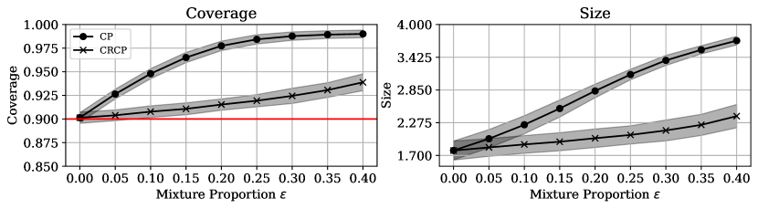
Figure 2: Coverage and size for standard conformal prediction (CP) and Contamination Robust Conformal Prediction (CRCP) in the logistic regression example with the LR model, and varying $\epsilon$. The red line in the left panel indicates the target 90% coverage and the shaded regions indicate one standard deviation.

5.2 Real Data with Label Noise

Here we illustrate CRCP on the contaminated CIFAR-10 dataset known as CIFAR-10N introduced in Wei et al. (2022). For this dataset, 3 independent workers were asked to assign labels to CIFAR-10 datasets collected from Amazon Mechanical Turk; for details see Wei et al. (2022). The CIFAR-10 dataset contains 60,000 colour images in 10 classes (such as airplane, automobile, bird), with 6,000 images per class. There are 50,000 training images and 10,000 test images. There are six sets of labels provided for each training image representing different noise patterns:

• Clean: This is the CIFAR-10 H dataset from Peterson et al. (2019) which is assumed to have a noise rate of 0 %.

• Aggr: In this dataset the label is assigned by majority voting, and picked randomly from the three submitted labels when there is no majority. These labels have a noise rate of 9.03%.

• R1: The assigned noisy label is the first submitted label for each image. These labels have a noise rate of 17.23%.

• R2: The assigned noisy label is the second submitted label for each image. These labels have a noise rate of 18.12%.

• R3: The assigned noisy label is the third submitted label for each image. These labels have a noise rate of 17.64%.

• Worst: If there are any wrongly annotated labels then the worst label is randomly selected from the wrong labels. These labels have a noise rate of 40.21%.

For each dataset we use the estimates for $P_{i}$ and $\tilde{P}_{i}$, for $i=1,\ldots,K$, as well as the matrix $P$, obtained in Wei et al. (2022) and based on empirical frequencies (using the notation from Section 3.4). In this example it is assumed that CIFAR-10H is the ground truth, so that the empirical distributions of the clean labels are available, and the matrix $P$ can be estimated.

In a more general context, the empirical frequencies of $\tilde{P}_{i}$ are directly available from the observations. The estimation of the matrix $P$ can be carried out for example as in Zhu et al. (2022). Estimating the distribution for the true labels may be not as straightforward. It is possible that this distribution is known from previous studies, or one may be able to assume that the true and the corrupted labels have the same marginal distribution, with the difference between the two distributions being that the true labels are related to the features of the data, whereas the corrupted labels are not related to the features.

We split the 50,000 images that have noisy, human-annotated labels into 20,000 images for training, 10,000 for validation, and 20,000 for calibration. For each of the six different label noise settings, we fine-tune a pre-trained ResNet-18 (He et al., 2016) model using the training and validation sets (see Appendix A.2 for details). For each repetition we subsample 10,000 calibration data from the remaining 20,000 images with human-annotated labels to calibrate the conformal prediction procedures, and subsample 5,000 test data from the provided set of 10,000 images which were not humanly annotated to evaluate the constructed prediction sets. Similar to the synthetic experiments, we perform 25 repetitions of this experiment with different seeds, and display the results in Table 2.

At a desired coverage of 90%, for the clean data both CP and CRCP achieve within two standard deviations of the desired coverage. For noisy data, though, with increasing noise ratio the standard CP obtains considerable over-coverage, while CRCP stays within two standard deviations of the desired noise level even for dataset with the highest noise level. Moreover the prediction intervals obtained by CRCP are considerably narrower, and hence more precise, than those obtained by CP.

Noise Type	CP		CRCP
	Coverage	Size	Coverage	Size
Clean	0.900 ± 0.005	1.507 ± 0.019	0.909 ± 0.005	1.507 ± 0.019
Aggr	0.940 ± 0.003	2.003 ± 0.027	0.899 ± 0.005	1.550 ± 0.019
R1	0.973 ± 0.002	2.997 ± 0.053	0.902 ± 0.005	1.672 ± 0.022
R2	0.977 ± 0.002	3.177 ± 0.066	0.903 ± 0.006	1.658 ± 0.021
R3	0.973 ± 0.002	3.042 ± 0.079	0.898 ± 0.006	1.636 ± 0.027
Worst	0.990 ± 0.001	5.473 ± 0.078	0.917 ± 0.009	2.189 ± 0.093

Table 2: Coverage and width of prediction intervals, $\pm$ 1 standard deviation, for prediction intervals aiming for 90% coverage, for standard conformal prediction (CP) and for Contamination Robust Conformal Prediction (CRCP) on the CIFAR-10N dataset. CRCP gives prediction intervals which are very close to the desired 90% coverage across all noise levels, and does not over-cover too much even in the noiseless case, while CP intervals show considerable over-coverage on all but the noiseless data. Moreover the CRCP intervals are narrower than the CP intervals.

6 Discussion

We start this section by discussing two papers that are closely related to this work, before positioning our work in the wider literature.

Non-Exchangeable Conformal Prediction

In recent work, Barber et al. (2023) extended conformal prediction to the non-exchangeable setting using a data re-weighting approach. They suppose that a data-independent weight $w_{i}\in[0,1]$ is applied to each score, and construct prediction sets using a weighted quantile $\widehat{C}_{n}\left(X_{n+1}\right)=\left\{y\in\mathcal{Y}:S\left(X_{n+1},y\right)\leq\mathrm{Q}_{1-\alpha}\left(\sum_{i=1}^{n}w_{i}\cdot\delta_{S_{i}}+w_{n+1}\cdot\delta_{+\infty}\right)\right\}.$ They show that, for calibration data that is independent, the prediction sets constructed using the weighted approach have the following coverage guarantee

$$\mathbb{P}\left(Y_{n+1}\in\widehat{C}_{n}\left(X_{n+1}\right)\right)\geq(1-\alpha)-\frac{\sum_{i=1}^{n}w_{i}\cdot\mathrm{d}_{TV}\left(S_{i},S_{n+1}\right)}{1+\sum_{i=1}^{n}w_{i}};$$ (40)

see Theorem 2 and Appendix A of Barber et al. (2023). Here, $d_{TV}$ denotes total variation distance; for two distributions $Q_{1}$ and $Q_{2}$ on $\mathbb{R}$ equipped with its Borel $\sigma$-field $\mathcal{B}$, $d_{TV}(Q_{1},Q_{2})=\sup_{A\in\mathcal{B}}|Q_{1}(A)-Q_{2}(A)|.$ In particular if the data is exchangeable and all the weights $w_{i}=1$ (as in standard conformal prediction) then (40) recovers the usual coverage guarantee.

The theory of non-exchangeable conformal prediction can be used to derive bounds on coverage in terms of the total-variation distance $d_{TV}$ in the contamination model introduced in Section 3, as follows. For the contamination model in Section 3 with $\Pi=(1-\epsilon)\Pi_{1}+\epsilon\Pi_{2}$ let $d_{\rm{diff}}=d_{TV}(\Pi_{1},\Pi_{2})$, and let $N$ be the number of corrupted points that appear in the calibration set, which is distributed as a $Bin(n,\epsilon)$ random variable, with mean $n\epsilon$. By Equation (40) with unit weights we have ${{\mathbb{P}}}(Y_{n+1}\in\widehat{C}_{n}(X_{n+1})|N=k)\geq 1-\alpha-\frac{2k}{n+1}d_{\rm{diff}}$ and so

$${{\mathbb{P}}}(Y_{n+1}\in\widehat{C}_{n}(X_{n+1})) =\sum_{k=0}^{n}{{\mathbb{P}}}(Y_{n+1}\in\widehat{C}_{n}(X_{n+1})|N=k){{\mathbb{P}}}(N=k)$$

$$\geq 1-\alpha-\frac{2}{n+1}d_{\rm{diff}}\sum_{k=0}^{n}k{{\mathbb{P}}}(N=k)=1-\alpha-\frac{2n\epsilon}{n+1}d_{\rm{diff}}\geq 1-\alpha-2\epsilon d_{\rm{diff}}.$$

A similar argument would give a matching upper bound. In comparison, our bounds in (3.1) use the weaker Kolmogorov-Smirnov ($d_{KS}$) distance. Not only is $d_{KS}\leq d_{TV}$, but it is also easier to compute; an extended discussion can be found in Adell and Jodrá (2006).

Appendix C in Barber et al. (2023) also provides a lower bound for the coverage probability which is comparable to the lower bound in Lemma 3.1; in the Huber contamination setting, the bound in Barber et al. (2023) improves on the lower bound in Lemma 3.1 when $d_{KS}(\Pi_{1},\Pi_{2})$ is large or, similarly, when ${{\mathbb{E}}}[F_{1}(\tilde{q})-F_{2}(\tilde{q})]$ is large, where large means larger than $\alpha/(1-\alpha)$.

Conformal Prediction under Label Noise

Einbinder et al. (2022) study the robustness of split conformal prediction in a related setting where it is assumed that the entire calibration set is observed under label noise. In the regression setting, this means noisy observations $S_{i}^{noisy}$ of the true scores $S_{i}$ are observed as $S^{noisy}_{i}=S_{i}+Z$ where $Z$ is a random variable. In contrast, our models as detailed in Section 3 consider the classical Huber contamination model in which some data are clean and only a fraction of the data are corrupted. As only continuously observed label noise is considered in Einbinder et al. (2022) they conclude that for regression, in all but pathological cases conformal prediction continues to provide coverage. They provide results similar to those introduced in Subsection 3.3, although they only consider the case where conformal prediction still provides (conservative) coverage and do not provide estimates for the coverage probabilities or efficiency.

Wider Related Works

Many works have addressed conformal prediction under different types of distribution shift including covariate shift (Tibshirani et al., 2019) and various different online or adversarial settings (Gibbs and Candes, 2021; Zaffran et al., 2022; Gibbs and Candès, 2022; Bastani et al., 2022). Our outlier setting can be seen as a specific case of distribution shift where the quantile is calibrated over a different distribution to the test data, and hence methodology from this literature could be used to address data corruption if it is known which of the observations are corrupted (an assumption which we do not make in this paper). A related approach is that of Cauchois et al. (2024), who study the distribution shift setting; here they propose to first estimate the magnitude of distribution shift between calibration and test data before utilising this estimate to adjust a conformal prediction procedure. While we assume that data corruptions are sampled from some unknown but fixed distribution, Gendler et al. (2022) consider the setting where the data is perturbed adversarially, and apply a randomized-smoothing approach to estimate an adjustment to recover coverage guarantees. In Angelopoulos et al. (2023), conformal prediction is extended to control the expectation of monotone loss functions, with one of the examples being transductive learning with a special type of distributional shift, namely that the conditional distribution of $Y$ given $X$ remains the same in training and test domain. In this case the distributional shift reduces to a covariate shift, which can be tackled using a weighted procedure.

There are also related papers on group conditional coverage: if the group membership of each sample is known, this problem can be tackled by configuring different thresholds for the different groups (Jung et al., 2022; Gibbs et al., 2023). In our setting, there would be two groups: clean or contaminated. However, we assume that the group membership is not known.

Future Work

This paper has illustrated that conformal prediction may be misleading when the data follow a Huber-type contamination model. In the classification setting we were able to offer a remedy under additional assumptions , via Theorem 4.1. The proof relies heavily on the discrete nature of the problem, which gives rise to a binomial distribution; it is not immediately obvious how to generalise it to continuous settings. Yet, similar remedies may be possible in other settings, such as that of functional regression. Exploring these settings will be part of future work.

Acknowledgements.

The authors would like to thank Aleksandar Bojchevski, Tom Rainforth and Aaditya Ramdas for helpful discussions, and the anonymous reviewers for their insightful comments. G.R. acknowledges support from EPSRC grants EP/T018445/1, EP/W037211/1, EP/V056883/1, and EP/R018472/1. W.X. acknowledges support from EPSRC grant EP/T018445/1; he is also supported by the DFG (German Research Foundation) – EXC number 2064/1 – Project number 390727645.

Appendix A

A.1 Proof of the Bound (37)

We start by applying the Cauchy Schwarz inequality to obtain

$${{\mathbb{E}}}[(1+B)^{-\frac{3}{2}}]={{\mathbb{E}}}\left[\frac{1}{B+1}\sqrt{\frac{1}{B+1}}\right]\leq\sqrt{{{\mathbb{E}}}\left[\frac{1}{(B+1)^{2}}\right]{{\mathbb{E}}}\left[\frac{1}{B+1}\right].}$$

To bound ${{\mathbb{E}}}[(1+B)^{-2}]$, we use the notion of size bias distributions; a random variable $X^{s}$ has the size bias distribution of a nonnegative rv $X$ if and only if ${{\mathbb{E}}}Xf(X)={{\mathbb{E}}}X\,{{\mathbb{E}}}f(X^{s})$ for all measureable functions $f$. Using the notion of size biasing one can show that if $X_{n}\sim Bin(n,p),$ then $1+X_{n-1}$ has the $X_{n}$-size bias distribution (see, for example Arratia et al. (2019)). So $1+B$ has the $X_{n}$-size bias distribution with $p=\tilde{P}_{j}$. Moreover, $1/(1+x)^{2}\leq 2/(2+x)^{2}$ and

$${{\mathbb{E}}}(1+B)^{-2}\leq 2\,{{\mathbb{E}}}(2+B)^{-2} =\frac{2}{np}{{\mathbb{E}}}\frac{X_{n}}{(1+X_{n})^{2}}<\frac{2}{np}{{\mathbb{E}}}\left\{\frac{1}{(1+X_{n})}\right\}=\frac{2}{np}\frac{1}{(n+1)p}{{\mathbb{P}}}(X_{n}\geq 1)$$

where we used size biasing twice, once with $f(x)=\frac{1}{1+x}$ and the second time with $f(x)=\frac{1}{x}1(x\geq 1).$ Using that ${{\mathbb{E}}}\left[\frac{1}{B+1}\right]\leq\frac{1}{n\tilde{P}_{i}}$(see Storey et al. (2003), Lemma 3), gives ${{\mathbb{E}}}[(1+B)^{-\frac{3}{2}}]\leq\sqrt{2}(n\tilde{P}_{j})^{-\frac{3}{2}},$ yielding (37). $\hfill\Box$

A.2 Experimental Details for Section 5

For both the synthetic and CIFAR-10N experiments we used the implementation of the APS scoring function provided by the authors of the original paper (Romano et al., 2020). The experiments were run on a single machine with an AMD Ryzen 7 3700X 8-Core Processor and an NVIDIA GeForce RTX 2060 SUPER GPU. The total running time to reproduce all the synthetic experiments in the paper is around 8 hours, and for the CIFAR-10N it is about 2 hours in total on this hardware.

For the synthetic data experiments, the classifiers were implemented using the scikit-learn (Pedregosa et al., 2011) library and were trained using their default hyper-parameters.

For the CIFAR-10N experiments, we used the ResNet-18 model available in the torchvision library which is pretrained on the ImageNet database (available at https://pytorch.org/vision/main/models/generated/torchvision.models.resnet18.html), and replaced the final layer to match the number of classes, which is 10 in our case. We initialise the weights to those of a ResNet-18 pre-trained on the Imagenet dataset (also available in the torchvision library) and trained each model for 30 epochs using the Adam (Kingma and Ba, 2015) optimiser, using a batch size of $128$ and an initial learning rate of $1e^{-3}$, which is decayed by a factor of $10$ any time the training loss does not decrease for 3 epochs. We evaluate the validation loss every epoch, and pick the model with the lowest validation loss overall.

References

- Adell and Jodrá (2006) José A Adell and Pedro Jodrá. Exact Kolmogorov and total variation distances between some familiar discrete distributions. Journal of Inequalities and Applications, 2006:1–8, 2006.
- Angelopoulos and Bates (2021) Anastasios N Angelopoulos and Stephen Bates. A gentle introduction to conformal prediction and distribution-free uncertainty quantification. arXiv preprint arXiv:2107.07511, 2021.
- Angelopoulos et al. (2023) Anastasios Nikolas Angelopoulos, Stephen Bates, Adam Fisch, Lihua Lei, and Tal Schuster. Conformal risk control. In The Twelfth International Conference on Learning Representations, 2023.
- Arnold et al. (2008) Barry C. Arnold, N. Balakrishnan, and H. N. Nagaraja. A First Course in Order Statistics. Society for Industrial and Applied Mathematics, 2008.
- Arratia et al. (2019) Richard Arratia, Larry Goldstein, and Fred Kochman. Size bias for one and all. Probability Surveys, 16:1–61, 2019.
- Balasubramanian et al. (2014) Vineeth Balasubramanian, Shen-Shyang Ho, and Vladimir Vovk. Conformal Prediction for Reliable Machine Learning: Theory, Adaptations and Applications. Newnes, 2014.
- Barber et al. (2023) Rina Foygel Barber, Emmanuel J Candes, Aaditya Ramdas, and Ryan J Tibshirani. Conformal prediction beyond exchangeability. The Annals of Statistics, 51(2):816–845, 2023.
- Bastani et al. (2022) Osbert Bastani, Varun Gupta, Christopher Jung, Georgy Noarov, Ramya Ramalingam, and Aaron Roth. Practical adversarial multivalid conformal prediction. In Advances in Neural Information Processing Systems, 2022.
- Cauchois et al. (2024) Maxime Cauchois, Suyash Gupta, Alnur Ali, and John C Duchi. Robust validation: Confident predictions even when distributions shift. Journal of the American Statistical Association, pages 1–66, 2024.
- Chen et al. (2022) Sitan Chen, Frederic Koehler, Ankur Moitra, and Morris Yau. Online and distribution-free robustness: Regression and contextual bandits with huber contamination. In 2021 IEEE 62nd Annual Symposium on Foundations of Computer Science (FOCS), pages 684–695. IEEE, 2022.
- Clarkson (2023) Jase Clarkson. Distribution free prediction sets for node classification. In International Conference on Machine Learning, pages 6268–6278. PMLR, 2023.
- Einbinder et al. (2022) Bat-Sheva Einbinder, Stephen Bates, Anastasios N Angelopoulos, Asaf Gendler, and Yaniv Romano. Conformal prediction is robust to label noise. arXiv preprint arXiv:2209.14295, 2022.
- Gammerman et al. (1998) Alex Gammerman, Volodya Vovk, and Vladimir Vapnik. Learning by transduction. In 14th Conference on Uncertainty in Artificial Intelligence, 1998.
- Gendler et al. (2022) Asaf Gendler, Tsui-Wei Weng, Luca Daniel, and Yaniv Romano. Adversarially robust conformal prediction. In International Conference on Learning Representations, 2022.
- Gibbs and Candes (2021) Isaac Gibbs and Emmanuel Candes. Adaptive conformal inference under distribution shift. Advances in Neural Information Processing Systems, 34:1660–1672, 2021.
- Gibbs and Candès (2022) Isaac Gibbs and Emmanuel Candès. Conformal inference for online prediction with arbitrary distribution shifts. arXiv preprint arXiv:2208.08401, 2022.
- Gibbs et al. (2023) Isaac Gibbs, John J Cherian, and Emmanuel J Candès. Conformal prediction with conditional guarantees. arXiv preprint arXiv:2305.12616, 2023.
- He et al. (2016) Kaiming He, Xiangyu Zhang, Shaoqing Ren, and Jian Sun. Deep residual learning for image recognition. In Proceedings of the IEEE conference on computer vision and pattern recognition, pages 770–778, 2016.
- Huber (1964) Peter J Huber. Robust estimation of a location parameter. The Annals of Mathematical Statistics, pages 73–101, 1964.
- Huber (1965) Peter J Huber. A robust version of the probability ratio test. The Annals of Mathematical Statistics, pages 1753–1758, 1965.
- Huber and Ronchetti (2011) Peter J Huber and Elvezio M Ronchetti. Robust Satistics. John Wiley & Sons, 2011.
- Jung et al. (2022) Christopher Jung, Georgy Noarov, Ramya Ramalingam, and Aaron Roth. Batch multivalid conformal prediction. In International Conference on Learning Representations, 2022.
- Kingma and Ba (2015) Diederik P. Kingma and Jimmy Ba. Adam: A method for stochastic optimization. In Yoshua Bengio and Yann LeCun, editors, 3rd International Conference on Learning Representations, ICLR 2015, San Diego, CA, USA, May 7-9, 2015, Conference Track Proceedings, 2015.
- Massart (1990) P. Massart. The tight constant in the Dvoretzky-Kiefer-Wolfowitz Inequality. The Annals of Probability, 18(3):1269 – 1283, 1990.
- Pedregosa et al. (2011) F. Pedregosa, G. Varoquaux, A. Gramfort, V. Michel, B. Thirion, O. Grisel, M. Blondel, P. Prettenhofer, R. Weiss, V. Dubourg, J. Vanderplas, A. Passos, D. Cournapeau, M. Brucher, M. Perrot, and E. Duchesnay. Scikit-learn: Machine learning in Python. Journal of Machine Learning Research, 12:2825–2830, 2011.
- Peterson et al. (2019) Joshua C Peterson, Ruairidh M Battleday, Thomas L Griffiths, and Olga Russakovsky. Human uncertainty makes classification more robust. In Proceedings of the IEEE/CVF international conference on computer vision, pages 9617–9626, 2019.
- Romano et al. (2020) Yaniv Romano, Matteo Sesia, and Emmanuel Candes. Classification with valid and adaptive coverage. In H. Larochelle, M. Ranzato, R. Hadsell, M.F. Balcan, and H. Lin, editors, Advances in Neural Information Processing Systems, volume 33, pages 3581–3591, 2020.
- Stankeviciute et al. (2021) Kamile Stankeviciute, Ahmed M Alaa, and Mihaela van der Schaar. Conformal time-series forecasting. Advances in Neural Information Processing Systems, 34:6216–6228, 2021.
- Storey et al. (2003) John D. Storey, Jonathan E. Taylor, and David Siegmund. Strong control, conservative point estimation and simultaneous conservative consistency of false discovery rates: a unified approach. Journal of the Royal Statistical Society Series B: Statistical Methodology, 66(1):187–205, 12 2003.
- Stute (1986) Winfried Stute. On almost sure convergence of conditional empirical distribution functions. The Annals of Probability, 14(3):891 – 901, 1986.
- Tibshirani et al. (2019) Ryan J Tibshirani, Rina Foygel Barber, Emmanuel J Candès, and Aaditya Ramdas. Conformal prediction under covariate shift. In Proceedings of the 33rd International Conference on Neural Information Processing Systems, pages 2530–2540, 2019.
- Vovk et al. (2005) Vladimir Vovk, Alex Gammerman, and Glenn Shafer. Algorithmic Learning in a Random World. Springer-Verlag, Berlin, Heidelberg, 2005.
- Wei et al. (2022) Jiaheng Wei, Zhaowei Zhu, Hao Cheng, Tongliang Liu, Gang Niu, and Yang Liu. Learning with noisy labels revisited: A study using real-world human annotations. In International Conference on Learning Representations, 2022.
- Zaffran et al. (2022) Margaux Zaffran, Olivier Féron, Yannig Goude, Julie Josse, and Aymeric Dieuleveut. Adaptive conformal predictions for time series. In International Conference on Machine Learning, pages 25834–25866. PMLR, 2022.
- Zargarbashi et al. (2023) Soroush H Zargarbashi, Simone Antonelli, and Aleksandar Bojchevski. Conformal prediction sets for graph neural networks. In International Conference on Machine Learning, pages 12292–12318. PMLR, 2023.
- Zhu et al. (2022) Zhaowei Zhu, Jialu Wang, and Yang Liu. Beyond images: Label noise transition matrix estimation for tasks with lower-quality features. In International Conference on Machine Learning, pages 27633–27653. PMLR, 2022.