Towards Human-Like Driving: Active Inference in Autonomous Vehicle Control

Abstract

This paper presents a novel approach to Autonomous Vehicle (AV) control through the application of active inference, a theory derived from neuroscience that conceptualizes the brain as a predictive machine. Traditional autonomous driving systems rely heavily on Modular Pipelines, Imitation Learning, or Reinforcement Learning, each with inherent limitations in adaptability, generalization, and computational efficiency. Active inference addresses these challenges by minimizing prediction error (termed ”surprise”) through a dynamic model that balances perception and action. Our method integrates active inference with deep learning to manage lateral control in AVs, enabling them to perform lane following maneuvers within a simulated urban environment. We demonstrate that our model, despite its simplicity, effectively learns and generalizes from limited data without extensive retraining, significantly reducing computational demands. The proposed approach not only enhances the adaptability and performance of AVs in dynamic scenarios but also aligns closely with human-like driving behavior, leveraging a generative model to predict and adapt to environmental changes. Results from extensive experiments in the CARLA simulator show promising outcomes, outperforming traditional methods in terms of adaptability and efficiency, thereby advancing the potential of active inference in real-world autonomous driving applications.

I Introduction

As the demand for fully Autonomous Vehicles (AVs) continues to push the boundaries of technology, the integration of sophisticated decision-making frameworks that can effectively mimic human cognitive processes becomes imperative. The development of autonomous driving systems has traditionally relied on methodologies such as Modular Pipeline (MP) [3], Imitation Learning (IL) [4][5], Reinforcement Learning (RL) [6], and direct perception [7]. Each of these approaches, while contributing valuable insights and capabilities, also presents distinct limitations in scalability, adaptability, and integration complexity. For instance, MPs, although highly interpretable and modular, suffer from error propagation and rigidity. IL can mimic expert behavior but struggles with generalization to unseen scenarios. RL offers the ability to learn from interaction but at the cost of sample inefficiency and computational demands.

Among the various approaches explored, the principle of active inference emerges as a promising paradigm, inspired by theories of human brain function. Active inference suggests that the brain continuously predicts sensory inputs and minimizes the difference between expected and actual signals through perception and action. This framework, grounded in the Free Energy Principle (FEP)[1], suggests a robust method for handling the uncertainties inherent in real-world driving environments. Active inference [8], a theory originally from neuroscience, is applied across a spectrum of fields including psychology, cognitive science, artificial intelligence, robotics, and AVs. This theory conceptualizes the brain as a predictive machine that continuously constructs and updates a generative model—encompassing hidden states, observations, and actions—using Bayesian inference to mirror the actual generative processes of the world. The primary aim of active inference is to minimize the gap between these predictions and sensory inputs, a discrepancy known as “surprise” in the literature, which is considered the upper bound for Free Energy (FE) [2]. The prediction error, or surprise, can be minimized in two distinct ways: 1) by refining the internal model of the world—often referred to as perception—to better align with the sensory input, or 2) by taking actions that alter the environment in such a way that the sensory inputs become more congruent with the internal model held by the brain.

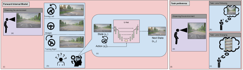
Figure 1: The overview of our method

In contrast to traditional methodologies, active inference offers a unified framework that seamlessly integrates perception and action, guided by a generative model that anticipates environmental changes. This approach enables an autonomous system to not just react to the environment but to engage with it in a predictive manner, learning a goal-directed task more human-like to mitigate the inherent problems of MP, IL, and RL.

This paper introduces a novel application of active inference to the lateral control of self-driving vehicles within a simulated urban environment. We propose a model that not only learns to predict the consequences of specific actions on the vehicle’s trajectory but also adapts to new road conditions without extensive retraining. By leveraging a deep learning architecture integrated with active inference, we demonstrate the model’s capability to perform driving maneuvers under varied urban structures.

Our approach leverages the principles of active inference to achieve computationally efficient, and explainable. By focusing on minimizing FE through action—adjusting the vehicle’s maneuvers to reduce prediction errors—our model demonstrates enhanced adaptability and performance in different driving scenarios. An overview of our method is shown in Fig.1. As can be seen, the decision-making of the car is done based on the current state of the world (input image is considered as the state for our case) and the prior knowledge of the world (internal world model) and how it changes based on different actions in the environment.

To the best of our knowledge, we are the first one who consider the active inference for the lateral control of self-driving vehicles in a simulator with an urban environment. Our model can generalize well as it learns the prior knowledge about how actions affect the environment. By doing a test on the new city that the agent did not see any image from, our model is able to predict the effect of steering on the image. So the performance of our model is not limited by an expert as it does not imitate the expert blindly and it kind of learns the logic under the agents’ decision making. In addition, the training part of the model is not that time consuming as we simplified the problem to only consider the road part of the image which matters for the decision making for the task of lane following. Ultimately, this work not only advances the technical capabilities of AVs but also deepens our understanding of how human-like cognitive processes can be emulated in artificial systems. This paper is structured as follows: it begins with a review of related works that establish the groundwork for our methodologies, followed by a description of our active inference-driven model, a detailed explanation of the simulated environments and experimental setups, and a presentation of results that validate the effectiveness of our approach in different urban landscapes, along with a discussion that contextualizes our findings within the broader landscape of autonomous driving research.

II Related Works

There are different methods for controlling an AV in an environment. One of the most popular methods is MP in autonomous driving systems which generally consists of dedicated modules for perception, prediction, planning, and control. While this approach offers clear advantages in terms of interpretability and modularity, it also has several limitations as follows. (i) Errors in upstream modules (e.g., perception) can propagate downstream, leading to compounding errors in prediction, planning, and control. This can significantly degrade the overall system performance. (ii) Integrating multiple modules from different sources can be complex and challenging. Ensuring smooth communication and coordination between modules often requires significant engineering effort. (iii) MPs can be inflexible, making it difficult to adapt the system to new tasks or environments without significant re-engineering. This rigidity can limit the scalability and versatility of the system. (iv) Each module is typically optimized independently, which can lead to sub-optimal overall performance. Joint optimization across modules is challenging due to the different nature of tasks each module performs [9][10].

Another method that is vastly used is Imitation Learning (IL) which has been a popular method for developing autonomous driving systems due to its ability to mimic expert behavior from demonstrations and a lot of work has been done in this domain [4][5][9][11][12]. Traditional IL methods, however, often struggle with generalizing to unseen states not covered by the expert’s demonstrations. When the agent encounters scenarios outside the training data, it may fail to perform adequately, leading to safety and reliability issues [9][13]. The IL performance heavily depends on the quality and quantity of expert demonstrations. Incomplete or sub-optimal demonstrations can lead to poor performance, as the agent can only replicate what it has seen during training. Unlike RL, IL does not promote environmental exploration or self-driven experimental learning, potentially restricting the agent’s capacity to adjust to new or changing environments.[10]. Additionally, in complex scenarios such as urban driving, high-level decisions (e.g. choosing to turn left or right at an intersection) cannot be inferred from perceptual input alone, leading to ambiguity and oscillations in the agent’s behavior. To overcome this, Codevilla et al.[9] introduced Conditional Imitation Learning (CIL), where the driving policy is conditioned on high-level commands. This approach allows the trained model to be guided by navigational commands during test time, thus enabling the vehicle to follow specific routes in urban environments. Their work showed that CIL could handle complex urban driving scenarios more effectively than traditional IL methods.

Direct perception methods are also the other category of methods that are used. Sauer et al. [14] propose Conditional Affordance Learning (CAL), a direct perception approach for autonomous urban driving. This method maps video inputs to intermediate representations (affordances) that are then used by a control algorithm to maneuver the vehicle. CAL aims to combine the advantages of MPs and IL by using a neural network to learn low-dimensional, yet informative, affordances from high-level directional inputs. The approach handles complex urban driving scenarios, including navigating intersections, obeying traffic lights, and following speed limits. However, choosing the best set of affordances is challenging. Furthermore, the effectiveness of this method relies heavily on precise affordance predictions. Any inaccuracies or errors in predicting affordances may result in less than optimal or even hazardous driving decisions.

Use of RL has shown promising results in training autonomous agents through trial and error[15][16][17]. However, it also has its own set of limitations. (i) RL methods typically necessitate extensive sample data to develop effective policies, which can be especially challenging in real-world settings where data acquisition is costly and time-intensive. (ii) Achieving a balance between exploration (testing new actions) and exploitation (leveraging known actions) presents a substantial hurdle in RL. Poor exploration strategies can lead to local optima and prevent the agent from discovering better policies. (iii) Designing appropriate reward functions is critical for RL but can be difficult and problem-specific. Poorly designed rewards can lead to unintended behaviors or sub-optimal performance. (iv) RL algorithms, particularly those that utilize deep learning, tend to be computationally intensive and demand significant computational resources. This requirement can restrict their use in environments where resources are limited. (v) Ensuring the stability and convergence of RL algorithms is challenging, especially in complex and dynamic environments. Instabilities during training can lead to unreliable and unpredictable agent behavior [9][10].

Liang et al.[17] introduce Controllable Imitative Reinforcement Learning (CIRL), which combines IL and RL to address the challenges of autonomous urban driving in complex, dynamic environments. CIRL utilizes a Deep Deterministic Policy Gradient (DDPG) approach to guide exploration in a constrained action space informed by human demonstrations. This method allows the driving agent to learn adaptive policies tailored to different control commands (e.g., follow, turn left, turn right, go straight). Despite using IL to guide initial exploration, CIRL still faces challenges associated with exploration in RL. The agent may struggle to discover optimal policies in highly dynamic and unpredictable environments without effective exploration strategies.

To adress these limitations of MPs ,IL, direct perception, and RL, we propose to use active inference that provides a robust framework that dynamically balances exploration and exploitation, adapts to new and unseen states, and minimizes prediction errors by choosing the best possible action. This approach allows for more adaptive and reliable autonomous systems capable of handling the complexities and uncertainties of real-world environments.

Active inference has been a growing area of interest in AV research. Friston et al. [18] established the theoretical foundations of active inference, proposing it as a process theory of the brain that minimizes prediction error or “surprise” by constantly updating its generative model or by inferring actions leading to less surprising states. This principle has been applied to various agents in simple simulated environments, but its application to realistic scenarios has been limited until recently. Catal et al. [19] introduced a novel approach by integrating deep learning with active inference for a real-world robot navigation task. They leveraged high-dimensional sensory data from camera frames to build complex generative models that operate without predefined state spaces. Their work demonstrated that deep active inference could successfully guide a mobile robot in a warehouse environment, showcasing the potential of this approach for real-world applications. However, they focused on a single, relatively controlled environment. de Tinguy et al. [20] presents a scalable hierarchical active inference model for autonomous navigation, exploration, and goal-oriented behavior inspired by human cognitive mapping strategies. The model integrates curiosity-driven exploration with goal-directed planning using visual observations and motion perception. It employs a multi-layered approach: from context to place to motion, allowing efficient navigation in new environments and rapid progress toward goals. They had a high success rate in goal-directed tasks with fewer steps required compared to other models. But, they only tested the validation of their method through simulations in a mini-grid environment. Nozari et al. [13] proposed a hybrid approach that combines active inference with IL to address the limitations of classical IL methods. Their framework uses a Dynamic Bayesian Network (DBN) to encode the expert’s demonstrations and incorporates an active learning phase where the autonomous agent refines its policy based on new experiences. This method allows the agent to dynamically balance exploration and exploitation, improving its adaptability to complex and dynamic environments. However, their method uses DBNs which introduce significant computational overhead, which may not be feasible for all autonomous driving platforms, particularly those with limited processing power or energy constraints.

III Method

III-A Active Inference Agent

Active inference is grounded in the FEP, which provides a mathematical framework for understanding how agents (biological or artificial) maintain a state of equilibrium with their environment. FEP is a fundamental principle that states organisms maintain their existence by minimizing their FE, which is a measure of surprise or prediction error. FE represents the difference between the predicted sensory inputs and the actual sensory inputs. Minimizing FE ensures that the organism’s internal model remains consistent with its sensory experiences, promoting adaptive behavior. As the FE might be intractable an approximation of it is used which is called Variational Free Energy (VFE) and provides a tractable way to perform Bayesian inference by optimizing an approximate posterior distribution.

The VFE can be expressed as

$$F=D_{KL}\left(Q(s)\parallel P(s\mid o)\right)-\log P(o),$$ (1)

where $D_{KL}$ is the Kullback-Leibler divergence, $Q(s)$ is the approximate posterior distribution over the hidden states $s$ given the observations $o$, and $P(s\mid o)$ is the true posterior distribution. The objective is to minimize the FE, ensuring that the approximate posterior $Q(s)$ is close to the true posterior $P(s\mid o)$, and reduces the surprise of observations under the model $P(o)$. Active inference extends this concept by incorporating a generative model that allows the agent to predict future states and observations. This model includes prior beliefs about how the environment behaves, and the agent uses these predictions to minimize FE through perception (updating beliefs) and action (changing state to reduce surprise). The VFE is minimized through two processes:

1. Perception (Inference): Updating beliefs to minimize prediction error.

2. Action (Control): Selecting actions that minimize Expected Free Energy (EFE), which includes both epistemic (information-seeking) and pragmatic (goal-directed) aspects.

In this work we tried to minimize the VFE using the action, while considering the expected future state (future image for our case) constant based on the task we have in hand. This can be done with the minimization of Expected Free Energy (EFE). The EFE $G$ at time $t$ can be expressed as

$$G=\mathbb{E}_{Q(o_{t},s_{t},a_{t})}\left[\log Q(s_{t},a_{t})-\log P(o_{t},s_{t},a_{t})\right],$$ (2)

where $\mathbb{E}_{Q(o_{t},s_{t},a_{t})}$ denotes the expectation under the approximate posterior distribution $Q$ over the observations $o_{t}$, hidden states $s_{t}$, and actions $a_{t}$ at time $t$, $\log Q(s_{t},a_{t})$ is the logarithm of the approximate posterior distribution over the hidden states $s_{t}$ and actions $a_{t}$ at time $t$, and $\log P(o_{t},s_{t},a_{t})$ is the logarithm of the true joint probability distribution over the observations $o_{t}$, hidden states $s_{t}$, and actions $a_{t}$ at time $t$. The equation essentially measures the expected divergence between the approximate posterior $Q$ and the true joint probability distribution $P$ over the variables of interest, guiding the agent’s behavior to minimize this discrepancy, where the environment is considered as a Partially Observable Markov Decision Process (POMDP).

In autonomous driving, active inference involves the agent (the vehicle) continuously predicting its sensory inputs (visual observations of the road) and minimizing the prediction error through either perception (updating its internal model) or action (steering adjustments). We used a forward internal model [30] for the perception part and for the action we used sensory-motor simulation (use of covert action).

Perception Model: For perception, we trained a forward internal model that contains all the information necessary for the agent to understand the environment in the context of the driving task. In this study, we assumed that the forward internal model, once learned offline, is comprehensive and does not require updating during the active inference agent training. This forward internal model is used to generate future images influenced by the steering angle. An overview of the forward internal model is depicted in Fig. 1. For learning forward internal model this paper uses a method inspired by [21]. As human beings, it is simple to predict how the environment will change based on the change of steering action as humans are really good at completely generating the missing information. However, it is not simple for a feed-forward neural network to predict details of the scene by providing one frame and the corresponding action when the future scene is too different from the current scene. The reason is that the network finds it hard to learn a good correlation between the current and the future scene even with the help of action. To the best of our knowledge, most literature available in future scene prediction based on action, considers normal driving scenarios [22][23] or simple environments like Atari games [24][25] in which the predicted images are still pretty much similar to the input image. Even for those cases, the models that are used cannot predict the future image without blurriness.

For the forward internal model, we used a U-Net Xception-style [31] model with modification for our task. We used the U-net [29] architecture due to multiple reasons. (i) U-Net is known to performs well with relatively fewer training examples. (ii) It can efficiently extracts hierarchical features from input images as it uses convolutional layers in both the encoding and decoding paths. (iii) It uses skip connections which help in preserving spatial information from early layers.

In our study, we observed increased blurriness when predicting future images for sharp steering angles, as the correlation between the input image and the prediction decreased. Since these predicted frames are crucial for solving the control problem, blurry images are not useful. Therefore, we cropped the image to focus only on the most informative parts relevant to decision-making, excluding areas unrelated to the driving task. We also considered using semantic segmented images and the road-only labels from these images. While semantic segmentation could potentially enhance the control task, it would introduce additional complexity and computational overhead that are unnecessary for low-level control tasks. Furthermore, using semantic segmentation to define preferred states (preferences [27]) presents challenges in incorporating environmental information unrelated to driving as this approach can make comparisons sensitive to changes in background scenes, such as variations between greenery or mountainous terrain along the road. So, we used road-only part of semantic segmented images for our control task.

For the data collection, a special strategy was used. As diverse data with various steering angles is needed to make the model learn about how steering affects the representation of the environment, the vehicle was driven in a zigzag pattern so that all different steering from -1 to 1 can be included in the data.

We used CARLA (Car Learning to Act) [26] simulator due to the realistic environment it provides for developing, training, and validating autonomous driving technologies in urban settings. The data was collected in Town06 of the CARLA simulator due to its structured highway layout, which enables rigorous testing of the robustness of our method across various lane configurations. For the training, different numbers of future images were tested regarding the action to consider the right causality (prediction of the next future image, third future image, fourth future image, and fifth future image were tested). The test result for the prediction of only the next future image was less blurry, but the model almost learned nothing about the effect of the steering. For the prediction of third, forth, and fifth future images the effect of steering on the result could be seen for image comparison. Some of the predicted results for semantic segmented images with their regarding ground truth are shown in Fig. 2. Also, the result for the grayscale road-only is shown in the Fig. 3.

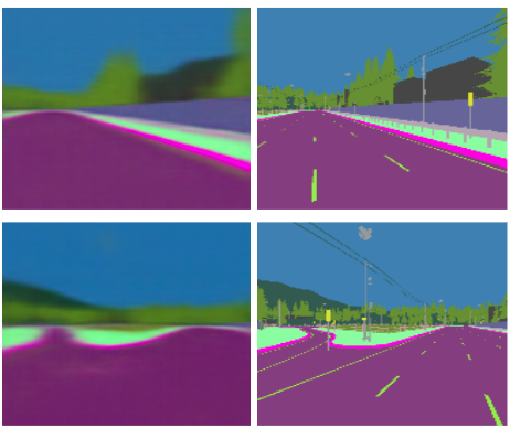
Figure 2: Predicted and the ground truth image for semantic segmented images

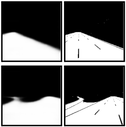
Figure 3: Predicted and the ground truth image for road-only images, using the grayscale road-only part of semantic segmented images to avoid complexity, computational overhead, and sensitivity to environmental variations.

The key advantage of using either the road-only part or the entire semantic segmented image is that the learned impact of actions on the predicted image can be applied to different cities without requiring additional training data for the new environment. The only adjustment needed is change of the preference. Although, driving becomes somewhat jerky when the car enters an intersection due to the comparatively lower amount of intersection data in the dataset, the car is still able to navigate through intersections even when there are no lane markings present.

Action Selection: The agent selects actions that minimize the EFE. This can be framed as

$$a_{t}=\arg\min_{a}G,$$ (3)

where G is the EFE as defined in equation (2). This approach allows the vehicle to adapt its driving behavior in real-time, making steering adjustments that minimize prediction errors. By leveraging the principles of active inference, the vehicle can learn human-like driving, effectively handling dynamic and uncertain road conditions. To minimize G, we use covert actions to imagine future states caused by the actions. Despite other methods that are used in AVs, our method more closely imitates human behavior in driving a car. For controlling a vehicle in the world, humans possess certain prior knowledge also called preference. This includes understanding how the world responds to their actions which is done by the forward internal model. For example, in driving, a human driver anticipates how steering affects the upcoming scene. If an AV is designed to mimic human intelligence, it must also be equipped with this knowledge.

In this paper, the steering is considered as the action (considering constant speed for simplicity) and the future scene is predicted based on the current scene and the action. After providing the prior knowledge of how different steering affects the future scene for the AV by the forward internal model, the expectation of the future should also be provided so that the model will be able to compare the internal state with the prediction and try to minimize the EFE. preference shows how the future should be regarding the task that the AV is doing. For instance, what the future road should be like is known considering a straight road in the same lane if the lane following task is being done. Considering the current state and the forward internal model, the action is then determined based on the highest similarity measure with the output that is expected (preference) in the environment (for the lane following task it will be the same as a straight view of the scene) and different possible future images based on different actions. For the lane changing, only the image with the view of the final lane that the vehicle should be in can be provided, however, if this is done the vehicle will do a sharp turn in order to minimize the EFE. So to have a smoother turn from one lane to another lane, different images that make the different steps for the lane changing task can be provided. In this study, we only considered the lane-following task but the lane-changing task also can be achieved based on our experiments which we will more specifically consider in our future studies. The similarity measure used in this work was the structural similarity index measure (SSIM [32]) as it leads to better driving performance. This minimization can be considered the same thing as the minimization of the EFE because it can be conceptually shown that this maximization of the similarity measure makes the surprise lower as the output would be as expected. Also, considering the Equation (2), we can consider the $Q(s_{t},a_{t})$ as the output of the covert action and the $P(o_{t},s_{t},a_{t})$ as our preference image. So, we are trying to minimize this difference by choosing the action that leads to a similar output as the preference.

After testing on the image level to see how different trained models are responsive to different steering, and how much blurriness the predicted image has, a test scenario was tried in the CARLA simulator. In the test scenario the car drives with the steering predicted with the help of the model using covert action to find an optimal action. As mentioned, the model predicts the future image with respect to the steering command. Twenty different steering between -1 and 1 were used with the step size of 0.1 and predicted the future image for each one. An overview of this comparison is shown in Fig. 4.

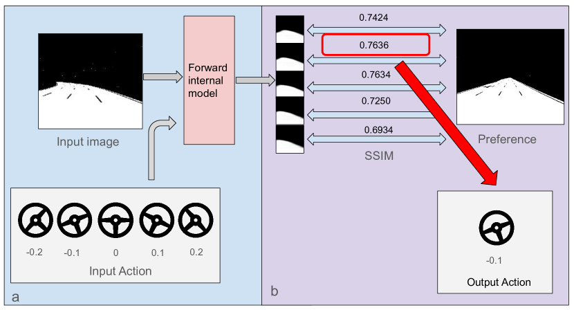
Figure 4: The overview of comparison for action prediction

Then the predicted images were compared with the preference for the task. To do this comparison, two different metrics were tested, namely MSE and SSIM. If the SSIM score was highest or the MSE was lowest while comparing all 20 images with the preference, the car would take the action that is done for the prediction of that image. This way, an action for each input image is available and the car can drive in the simulator. The fourth future image in a constant speed was used for driving in the simulator.

III-B Imitation Learning Agent

In this study, we adopt IL (more specifically Behavioral Cloning (BC) as our baseline method for several compelling reasons. (i) BC offers a straightforward approach to learning policies from expert demonstrations, requiring minimal additional infrastructure beyond the demonstration data itself. This simplicity not only facilitates rapid implementation but also serves as a foundational benchmark against which more complex algorithms can be evaluated. By establishing BC as our baseline, we aim to provide a clear reference point for assessing the efficacy of our active inference based method. (ii) As the BC only needs the camera images, we do not need to consider other sensors input and the comparison would be fair as both active inference method that we proposed in our work and the BC use the same sensor. (iii) Due to the use of the same sensor input (single camera) the size of the data for both methods can be the same.

IV Experimental Setup

IV-A Network Architecture and Trainig

IV-A1 Active Inference

We used a U-Net Xception-style model [28] in keras. The input image was encoded with the encoding part of the U-Net and then the action was added (which is only steering for in this case) by concatenating the action through Dense layers. For this task, the upsampling layers are changed to the conv2d_transpose layer as they can make the reconstructed image less blurry. In addition, as only the road part of the image is considered, grayscale images are used. So, one channel in both the input layer and output layer is used. The input and output images have the same size of $160\times 160\times 1$. The RELU activation function is used for encoding and decoding layers and the ELU activation function is used for the part where the action was added. For the output layer, the sigmoid activation function was used. A learning rate of 1e-4 and batch size of 128 were used to train this model.

IV-A2 Imitation Learning

We used the same size cropped images for training the BC agent as we used for the active inference agent. The model that was used for training the BC agent is shown in Table I. A learning rate of 1e-3 and batch size of 64 were used to train this model.

TABLE I: Neural Network Architecture used for the BC agent

Layer Type	Description	Kernel Size / Units	Activation
Input	Input Image	(160, 160, 3)	-
Conv2D + BN	32 filters, stride 2	5x5	ReLU
Conv2D + BN	64 filters, stride 2	3x3	ReLU
Conv2D + BN	128 filters, stride 2	3x3	ReLU
Dropout	20% rate	-	-
Conv2D + BN	256 filters, stride 2	3x3	ReLU
Flatten	Flatten	-	-
Dense	Fully connected	512	ReLU
Dropout	20% rate	-	-
Dense	Fully connected	128	ReLU
Dropout	20% rate	-	-
Dense	Fully connected	64	ReLU
Dense	Fully connected	1	-

IV-B Simlutator and Dataset

CARLA has different versions that provide different cities and structures. The stable version of CARLA which is 0.8.4 only supports two towns, but 0.9.X versions support more towns. As an example the version 0.9.14 that we have used in our work supports eight different towns. For the simulation, two different versions of the CARLA simulator were used. The version 0.9.14 is used for our test scenario which occurred in two different towns, Town04 and Town06. We compared the driving of our agent in Town04, Town06, and Town01 with an BC agent. For comparison, different tracks on Town01, Town04, and Town06 of CARLA simulator were randomly chosen and used. The used tracks are shown in the Fig. 6, Fig. 7, and Fig. 5: Here, three different tasks were considered for comparing different behaviors of the agents. For each of the tasks in Town04 and Town06 there are four different lanes that the car is tested in. The test in different lanes was done to see how robust the algorithm is against different lanes in the environment.

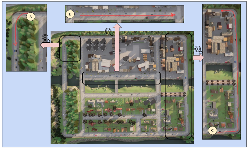
Figure 5: Tracks used for testing in Town01. A shows the one-turn, B shows the straight, and C shows the two-turn track.

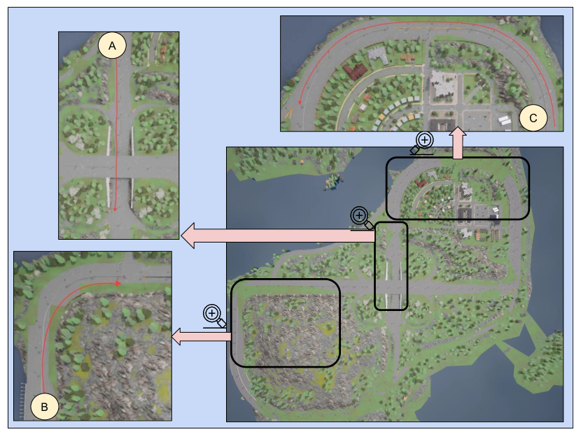
Figure 6: Tracks used for testing in Town04. A shows the straight track, B shows the one-turn track, and C shows the two-turn track.

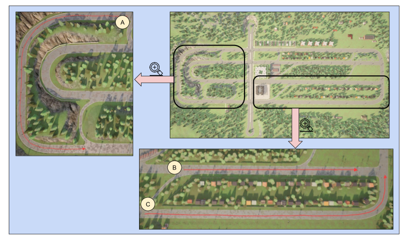
Figure 7: Tracks used for testing in Town06. A shows the two-turn track, B shows the straight track, and C shows the one -turn track.

IV-B1 Active Inference

We collected 36,000 images in Town06, and the data was augmented with the flipping and the change of the sign of regarding steering angle, which made the data 72,000 images and steering pairs. The distribution of the data is shown in the Fig. 8.

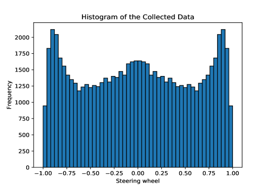
Figure 8: Distribution of the training data for the forward internal model

Images that were used as the preference for the active inference agent for both Town04 and Town06 are shown in Fig. 9, and 10 respectively. Each image shows the lane1-4 from left to right for each town. Different preferences were used for each town because the structure of the towns varied mostly on the side of the lane. This way our method can be adapted to be used for different towns. For the experiments done on Town01 and Town02 (used in the benchmark), we used the image shown in Fig. 11 as an preferences for both towns. This is mainly because when we tried to have different preferences in both towns we realized that the preferences in these two towns are almost identical. We have done two different tests for comparing our new active inference-based method to the other works done. The first test was done on different tracks of Town06, Town04, and Town01 to compare our method to BC. Another test was done on the CARLA simulator on the CoRL2017 [26] benchmark. This benchmark was used as our active inference-based AV could not consider challenging scenarios when other dynamic objects are in the scene as it was not trained to do so as well. So, other benchmarks such as Nocrash and Leaderboard1, Leaderboard2 were not useful for testing this work. For this benchmark CARLA version 0.8.4 was used as this benchmark is only supported in the previous versions of CARLA and not the version 0.9.14 which was used in this work. The result of this benchmark is shown in Table IV.

The CoRL2017 only considered the RGB image for testing different methods. But as we were using the road-only part, we added a semantic segmentation camera to it and used the data from this camera instead of RGB camera to be able to test our method. Here, both Town01 and Town02 can be considered as test towns as the training data was from the Town06 of the CARLA simulator. Also only one weather condition was used for training data which is the default weather in Town06. However, based on the CARLA documentation and our observation the semantic segmented images are not affected by different weather conditions and only RGB sensor data will be affected by it, which we do not use in our work. To have a fair comparison only the trained weather condition was considered while comparing our method to others.

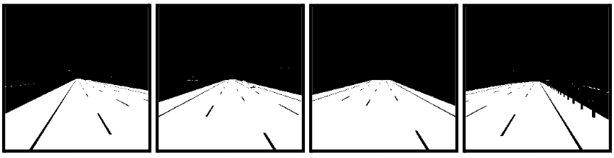
Figure 9: Town04 preferences that shows the lanes 1-4 from left to right

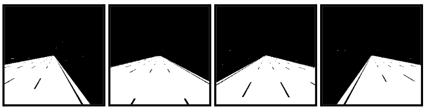
Figure 10: Town06 preferences that shows the lanes 1-4 from left to right

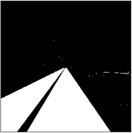
Figure 11: Town01 and Town02 preference

IV-B2 Imitation Learning

The BC agent was trained on a dataset collected from Town06 and was tested in all towns. Training of IL agents was not straightforward in Town06 as there are multiple lanes in the environment. We needed to collect enough data from multiple lanes in the simulator. Also, the car was prone to driving near the curb of the road in turns. Here, for a fair comparison, the BC agent was only trained to have lateral control. For good driving, we collected 61,000 data that were almost equally distributed from different lanes in the simulator. Even with the change in the brightness and the flip as the augmentation, the results were not satisfactory. So we added the flipped data to the dataset and normalized the data. Although the driving was better, it was not still good enough and the car had issues in turns on different tracks. Also, when the car went off the track, it could not come back to it. So, we collected 32,000 data of coming back to the track from different lanes. The final normalized dataset consists of 47,313 images with the steering angle. The histogram of the normalized data can be seen in Fig. 12.

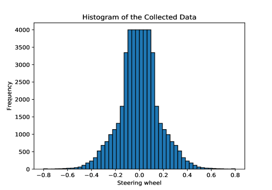
Figure 12: Histogram of the training data for the BC agent

V Results

TABLE II: Deviation Metrics for Different Tasks, Tracks, and Agents in Two Towns

Town	Task	Lane	Deviation
			BC	Active inference
Town04	Straight	Lane1	0.769	$0.335$
		Lane2	0.250	$1.533$
		Lane3	0.313	$0.571$
		Lane4	1.305	$0.809$
	One-Turn	Lane1	3.120	$0.598$
		Lane2	0.986	$0.921$
		Lane3	0.844	$0.954$
		Lane4	1.905	$1.303$
	Two-Turns	Lane1	1.513	$0.277$
		Lane2	0.330	$1.273$
		Lane3	0.421	$1.257$
		Lane4	1.233	$0.483$
Town06	Straight	Lane1	1.756	$0.406$
		Lane2	0.379	$1.019$
		Lane3	0.479	$0.877$
		Lane4	2.037	$0.501$
	One-Turn	Lane1	1.598	$0.358$
		Lane2	0.582	$0.938$
		Lane3	2.469	$0.809$
		Lane4	2.486	$0.187$
	Two-Turns	Lane1	1.685	$0.494$
		Lane2	1.209	$0.452$
		Lane3	1.152	$1.258$
		Lane4	1.869	$0.382$

V-A Performance Metric

Active inference proved to be a robust and adaptable agent for autonomous driving, as evidenced by the comprehensive analysis presented in Tables II and III. Across multiple tasks and urban environments, active inference consistently achieved superior performance compared to Behavioral Cloning (BC).In the tables deviation is the average value of the Euclidean distance between the vehicle’s positions and the corresponding waypoints, and the success rate shows, across different tracks, how many tracks were successfully completed. For each track, four different experiments were conducted, and the success rate was computed based on the success of these experiments.

V-A1 Town01 Performance

In Town01, active inference excelled with lower deviations and a 100% success rate in all tasks. For instance, in the One-Turn task, active inference had an average deviation of 0.540, while BC faced difficulties, particularly in the Straight and Two Turns tasks with deviations of 0.978 and 3.418, respectively, and success rates of 0% and 25%.

V-A2 Town04 Performance

In Town04, active inference demonstrated consistent performance with lower deviations and higher success rates in all tasks compared to BC. For the Straight task, active inference maintained an average deviation of 0.812 units and a success rate of 100%, while BC had a deviation of 0.688 units with the same success rate. Although in the Straight task the average deviation was better for the BC agent, the difference is insignificant. In the One-Turn task, active inference achieved an average deviation of 0.944 units and a 100% success rate, significantly outperforming BC which had a deviation of 1.714 units and a 0% success rate.

V-A3 Town06 Performance (Training Town)

In Town06, active inference maintained high performance with an average deviation of 0.573 units in the One-Turn task and a success rate of 100%. BC, on the other hand, had a deviation of 1.784 units for the same task but achieved a 100% success rate. For the Straight task, active inference recorded an average deviation of 0.701 units with a 75% success rate, whereas BC showed a higher deviation of 1.163 units with the same success rate.

TABLE III: Performance Metrics of Agents in Different Urban Environments Across Various Tracks

Town	Agent	Task	Avg. Dev.	Success (%)
Town01	Active inference	One-Turn	0.540	$100$
		Straight	0.408	$100$
		Two Turns	0.486	$100$
Town01	BC	One-Turn	1.217	$0$
		Straight	0.978	$0$
		Two Turns	3.418	$25$
Town04	Active inference	One-Turn	0.944	$100$
		Straight	0.812	$100$
		Two Turns	0.823	$100$
Town04	BC	One-Turn	1.714	$0$
		Straight	0.688	$100$
		Two Turns	0.875	$100$
Town06	Active inference	One-Turn	0.573	$100$
		Straight	0.701	$75$
		Two Turns	0.646	$100$
Town06	BC	One-Turn	1.784	$100$
		Straight	1.163	$75$
		Two Turns	1.479	$100$

TABLE IV: Success rate result in benchmark CoRL2017

Task	Town01							Town02
	MP[26]	IL[26]	RL[26]	CAL[14]	CIRL[17]	LBC [10]	Ours	MP[26]	IL[26]	RL[26]	CAL[14]	CIRL[17]	LBC [10]	Ours
Straight	98	95	89	100	98	100	96	92	97	74	93	100	100	92

V-B CoRL2017 Benchmark

We compared our results with different methods including MP, IL and RL which are introduced in CARLA simulator [26]. Moreover the results for papers CIRL [17], CAL [14], LBC [10] also shown in the Table IV. For these articles, Town01 is used as a training town and Town02 was used as a testing town. Although we simplified the problem, as this is a new method for learning and controlling the AV, we can assert that this new method can result in a comparable result as a more complicated method. Our method which follows the Active Inference principle is following a more human-like strategy with using the prior knowledge of how the world works by simulating the prior knowledge that humans can use as an imagination to see the effect of the action on the scene and deciding based on the desired future scene that they have in mind. Although based on the table, the result of our method for the straight task was better than IL and RL and slightly worse than the other methods, as we did not use any data from Town01 for training and these methods were using from this town for the training purposes, we can assert that our result is pretty good for this task. The results for Town02 shows that our agent driving is almost as good as CAL and MP methods and is better than the RL method. Although the result of our method is not as good as CIRL and LBC, the structure of our training is much more simpler than the one used in LBC as they use a two-stage training process that is more complex and resource-intensive. Also, CIRL uses a dual-stage learning process that introduces complexity in implementation and tuning. Balancing the IL and RL requires careful calibration to prevent issues like overfitting to the imitation data or insufficient generalization from the RL stage.

VI Conlusion

In this paper, we introduced a novel Active Inference-based method for controlling an autonomous vehicle, leveraging the Free Energy Principle (FEP) to dynamically adapt to different road types, including two-lane and multi-lane environments. Our method significantly enhances the adaptability and performance of AVs, achieving comparable results to more complex baseline methods in the CARLA benchmark.

Our results demonstrate that the Active Inference agent, despite its simplicity, performs robustly across various urban environments and driving tasks. It consistently outperforms Behavioral Cloning (BC) in terms of lower average deviations and higher success rates in simulated environments. This highlights the effectiveness of our approach in mimicking human-like driving behavior through the continuous minimization of prediction errors.

Notably, our method also showed competitive performance in the CoRL2017 benchmark, further validating its effectiveness. The success rates and deviation metrics indicate that our Active Inference-based agent can navigate complex scenarios effectively, maintaining human-like driving performance.

Future work will focus on extending the capabilities of our Active Inference-based agent to include tasks such as lane changing, handling dynamic objects in the driving scene, and adhering to traffic rules. Additionally, we aim to validate our approach using real-world data and explore its application to actual autonomous driving scenarios. By doing so, we hope to bridge the gap between simulation and real-world performance, ultimately advancing the field of autonomous vehicle control.

References

- [1] Friston, K., 2010. The free-energy principle: a unified brain theory?. Nature reviews neuroscience, 11(2), pp.127-138.
- [2] Friston, K.J. and Stephan, K.E., 2007. Free-energy and the brain. Synthese, 159, pp.417-458.
- [3] Badue, C., Guidolini, R., Carneiro, R.V., Azevedo, P., Cardoso, V.B., Forechi, A., Jesus, L., Berriel, R., Paixao, T.M., Mutz, F. and de Paula Veronese, L., 2021. Self-driving cars: A survey. Expert systems with applications, 165, p.113816.
- [4] D. A. Pomerleau. Alvinn: An autonomous land vehicle in a neural network. Technical report, DTIC Document, 1989.
- [5] Bojarski, M., Del Testa, D., Dworakowski, D., Firner, B., Flepp, B., Goyal, P., Jackel, L.D., Monfort, M., Muller, U., Zhang, J. and Zhang, X., 2016. End to end learning for self-driving cars. arXiv preprint arXiv:1604.07316.
- [6] Kendall, A., Hawke, J., Janz, D., Mazur, P., Reda, D., Allen, J.M., Lam, V.D., Bewley, A. and Shah, A., 2019, May. Learning to drive in a day. In 2019 international conference on robotics and automation (ICRA) (pp. 8248-8254). IEEE.
- [7] Chen, C., Seff, A., Kornhauser, A. and Xiao, J., 2015. Deepdriving: Learning affordance for direct perception in autonomous driving. In Proceedings of the IEEE international conference on computer vision (pp. 2722-2730).
- [8] Parr, T., Pezzulo, G. and Friston, K.J., 2022. Active inference: the free energy principle in mind, brain, and behavior. MIT Press.
- [9] Codevilla, F., Müller, M., López, A., Koltun, V. and Dosovitskiy, A., 2018, May. End-to-end driving via conditional imitation learning. In 2018 IEEE international conference on robotics and automation (ICRA) (pp. 4693-4700). IEEE.
- [10] Chen, D., Zhou, B., Koltun, V. and Krähenbühl, P., 2020, May. Learning by cheating. In Conference on Robot Learning (pp. 66-75). PMLR.
- [11] Xu, H., Gao, Y., Yu, F., Darrell, T.: End-to-end learning of driving models from large-scale video datasets. CVPR (2017)
- [12] J. Hawke, R. Shen, C. Gurau, S. Sharma, D. Reda, N. Nikolov, P. Mazur, S. Micklethwaite, N. Griffiths, A. Shah, et al., “Urban driving with conditional imitation learning,” in ICRA, 2020.
- [13] Nozari, S., Krayani, A., Marin-Plaza, P., Marcenaro, L., Gomez, D.M. and Regazzoni, C., 2022. Active inference integrated with imitation learning for autonomous driving. IEEE Access, 10, pp.49738-49756.
- [14] Sauer, A., Savinov, N. and Geiger, A., 2018, October. Conditional affordance learning for driving in urban environments. In Conference on robot learning (pp. 237-252). PMLR.
- [15] A. Kendall, J. Hawke, D. Janz, P. Mazur, D. Reda, J.-M. Allen, V.-D. Lam, A. Bewley, and A. Shah, “Learning to drive in a day,” in ICRA, 2019.
- [16] M. Toromanoff, E. Wirbel, and F. Moutarde, “End-toend model-free reinforcement learning for urban driving using implicit affordances,” in CVPR, 2020.
- [17] X. Liang, T. Wang, L. Yang, and E. Xing, “Cirl: Controllable imitative reinforcement learning for vision-based self-driving,” in ECCV, 2018.
- [18] Friston, K., Schwartenbeck, P., FitzGerald, T., Moutoussis, M., Behrens, T. and Dolan, R.J., 2013. The anatomy of choice: active inference and agency. Frontiers in human neuroscience, 7, p.598.
- [19] Çatal, O., Wauthier, S., Verbelen, T., De Boom, C. and Dhoedt, B., 2020. Deep active inference for autonomous robot navigation. arXiv preprint arXiv:2003.03220.
- [20] de Tinguy, D., Van de Maele, T., Verbelen, T. and Dhoedt, B., 2024. Spatial and Temporal Hierarchy for Autonomous Navigation Using Active Inference in Minigrid Environment. Entropy, 26(1), p.83.
- [21] Xiao, Y., Codevilla, F., Pal, C. and Lopez, A., 2021, October. Action-based representation learning for autonomous driving. In Conference on Robot Learning (pp. 232-246). PMLR.
- [22] Kwon, Y.H. and Park, M.G., 2019. Predicting future frames using retrospective cycle gan. In Proceedings of the IEEE/CVF Conference on Computer Vision and Pattern Recognition (pp. 1811-1820).
- [23] Zhu, D., Chern, H., Yao, H., Nosrati, M.S., Yadmellat, P. and Zhang, Y., 2018, November. Practical Issues of Action-Conditioned Next Image Prediction. In 2018 21st International Conference on Intelligent Transportation Systems (ITSC) (pp. 3150-3155). IEEE.
- [24] Oh, J., Guo, X., Lee, H., Lewis, R.L. and Singh, S., 2015. Action-conditional video prediction using deep networks in atari games. Advances in neural information processing systems, 28.
- [25] Wang, E., Kosson, A. and Mu, T., 2017. Deep action conditional neural network for frame prediction in Atari games. Technical report.
- [26] Dosovitskiy, A., Ros, G., Codevilla, F., Lopez, A. and Koltun, V., 2017, October. CARLA: An open urban driving simulator. In Conference on robot learning (pp. 1-16). PMLR.
- [27] Mazzaglia, P., Verbelen, T. and Dhoedt, B., 2021. Contrastive active inference. Advances in Neural Information Processing Systems, 34, pp.13870-13882.
- [28] kerashttps://keras.io/examples/vision/oxford_pets_image_segmentation/#prepare-unet-xceptionstyle-model
- [29] Ronneberger, O., Fischer, P. and Brox, T., 2015. U-net: Convolutional networks for biomedical image segmentation. In Medical image computing and computer-assisted intervention–MICCAI 2015: 18th international conference, Munich, Germany, October 5-9, 2015, proceedings, part III 18 (pp. 234-241). Springer International Publishing.
- [30] Wolpert, D.M., Ghahramani, Z. and Jordan, M.I., 1995. An internal model for sensorimotor integration. Science, 269(5232), pp.1880-1882.
- [31] F. Chollet, Xception: Deep learning with depthwise separable convolutions, arXiv:1610.02357 (2016).
- [32] Wang, Z., Bovik, A.C., Sheikh, H.R. and Simoncelli, E.P., 2004. Image quality assessment: from error visibility to structural similarity. IEEE transactions on image processing, 13(4), pp.600-612.