Metric mean dimension via subshifts of compact type
Abstract.
We investigate the metric mean dimension of subshifts of compact type. We prove that the metric mean dimensions of a continuous map and its inverse limit coincide, generalizing Bowen’s entropy formula. Building upon this result, we extend the notion of metric mean dimension to discontinuous maps in terms of suitable subshifts. As an application, we show that the metric mean dimension of the Gauss map and that of induced maps of the Manneville-Pomeau family is equal to the box dimension of the corresponding set of discontinuity points, which also coincides with a critical parameter of the pressure operator associated to the geometric potential.
Key words and phrases:
Metric mean dimension; Subshift; Box dimension2010 Mathematics Subject Classification:
Primary: 37D35, 28D20, 37B40, 37C85, 37B10.1. Introduction
Symbolic dynamics on finite alphabets are classical mathematical objects that have brought forward a great variety of dynamics and intervened in major achievements in Dynamical Systems and Ergodic Theory. The main invariant in these areas is the entropy, which may be expressed through both a topological and a measure-theoretical perspective. For subshifts on finite alphabets the topological entropy quantifies the exponential growth rate of the number of finite words of fixed length. Furthermore, for a Markov subshift the entropy equals the logarithm of the spectral radius of the generating graph, which may be read as the spectral radius of a linear operator.
For compact alphabets this interpretation of complexity in terms of counting words is no longer feasible. Nevertheless, we may still follow the same guiding principle by using a dimensional approach. More precisely, for a given scale, one identifies all but finitely many letters prior to counting and defines the entropy at that scale; the topological entropy is thus obtained by refining the scale. However, in this setting, its value may be infinite. The metric mean dimension introduced by E. Lindenstrauss and B. Weiss in [17] is a geometric invariant which is useful to distinguish precisely those systems with infinite topological entropy. It measures the speed at which the entropy at a given scale goes to infinity as the scale approaches zero, and it can be seen as a dynamical analogue of the box dimension. For example, the metric mean dimension of a full shift on a compact alphabet, endowed with a suitable metric, is exactly the box dimension of the alphabet.
There is an asymmetry in the definition of topological entropy since it looks only at the future orbits of points, and the same happens with the metric mean dimension. When the map is invertible, it turns out that its inverse has the same entropy. On the contrary, when the map is not invertible, the definition of entropy cannot be reversed in time. Yet, a non-invertible map induces a shift homeomorphism on the corresponding inverse limit space, and Bowen showed in [2] that the entropy of such a shift homeomorphism is equal to the entropy of the original map.
Generalizing the class of subshifts of finite type, Friedland introduced in [10] the analogous concept within the compact alphabet setting, which we refer to as subshifts of compact type, and proved that the topological entropy of the unilateral and bilateral subshifts induced by a fixed transition set coincide. This relation was already known for subshifts of finite type on finite alphabets, in which case the entropy is equal to the spectral radius of the transition matrix. In the particular case where the transition set is the graph of a continuous map, the associated bilateral subshift is a reformulation of the inverse limit of the map. Altogether, Friedland’s results generalize Bowen’s formula to arbitrary subshifts of compact type. In this paper we shall establish analogous properties for the metric mean dimension (see Theorems A and B). As a byproduct, we provide an upper bound for the metric mean dimension of an arbitrary map acting on a compact metric space in terms of spectral radii of scale-dependent matrices (see Section 6).
An application of our results, which is of independent interest, is that they motivate a definition of metric mean dimension for discontinuous maps on compact metric spaces in terms of suitable subshifts of compact type. To illustrate the scope of this new concept, we will show that the metric mean dimension of an interval map with infinitely many full branches coincides with the box dimension of its sets of critical points (see Theorem C). In particular, this setting comprises the Gauss map and the Young-induced maps of the Manneville-Pomeau family.
The paper is organized as follows. In the remainder of this section we will briefly recall a few definitions, state our main results and address some applications. In Sections 2 and 6 we collect some auxiliary material. Sections 3, 4, 5, 7 are devoted to the proofs.
1.1. Subshifts of compact type
Let be a compact metric space and or . In the rest of the paper, we fix some and endow the product space with the metric
| (1) |
A subset is called a subshift if it is closed and invariant by the shift action
We recall that the metric mean dimension of the full shift is given by (see the precise definitions in Section 2)
| (2) |
(see [23, Theorem 5] and also [6, Theorem D] for a version with potential).
Consider a subset , whose role will be to to prescribe transitions, and the induced set of admissible sequences
which is invariant and we always assume to be non-empty. We refer to as a subshift of compact type and note that is already closed whenever is. This model was proposed by Friedland (cf. [10]) in order to assign a notion of entropy to finitely generated free semigroup actions. We refer the reader to Section 4 for more information regarding such actions.
It was proved in [10, Theorem 3.1] that the topological entropy of the unilateral and bilateral subshifts induced by a given closed set coincide. Our first result shows that this also holds in the case of the metric mean dimension.
Theorem A.
Let be a compact metric space and be a closed subset. Then,
A particular instance to which we can apply Theorem A is when we consider and , where is a continuous map. In this case, the subshift
is refered to as the inverse limit of . In the entropy setting, Bowen’s formula is an immediate consequence of Friedland’s [10, Theorem 3.1], since and are topologically conjugate. Even though the metric mean dimension is not a topological invariant (though it is a bi-Lipschitz one), we show that it is the same for these two systems. The next result summarizes this information.
Theorem B.
Let be a compact metric space and be a continuous map. Then
| (3) |
Some comments are in order. Clearly, Theorem B hints that it is worthwhile investigating the metric mean dimension of subshifts on compact alphabets, a topic that has recently received much attention (see [12], [13], [22]), though far less known than the finite alphabet case. We remark that Theorems A and B were first proved in the author’s Master Thesis [18]. After completing this work, we became aware that a version of Theorem B for surjective maps was recently published in [3, Lemma 3.8].
Under apropriate adjustments, Theorem B allows us to extend properties valid for invertible maps to non-invertible ones. Let us illustrate this feature. Given a continuous map acting on a compact metric space , denote by the set of invariant Borel probability measures endowed with the weak∗ topology, and by its subset of ergodic elements. Consider the local metric mean dimension function introduced in [6], defined as
| (4) |
The map is upper semi-continuous and constant almost everywhere with respect to any ergodic probability measure (cf. [6, Lemmas 9.1 and 9.2]) and has been connected to different notions of measure-theoretic metric mean dimension (cf. [6, Corollary 9.6 and Example 10.5]). The next result was established in [6, Theorem E] under the assumption that the map is a homeomorphism. Using Theorem B, we may drop this condition.
Corollary 1.1.
Let be a compact metric space and be a continuous map such that . Then
| (5) |
In addition, a measure attains the previous maximum if and only if
An element is said to be a metric mean dimension point if ; it is a full metric mean dimension point if Denote the set of such points by and , respectively. The following is an immediate consequence of Corollary 1.1, which, in particular, guarantees the existence of full metric mean dimension points.
Corollary 1.2.
Let be a compact metric space and be a continuous map. Then there exists an ergodic probability measure such that
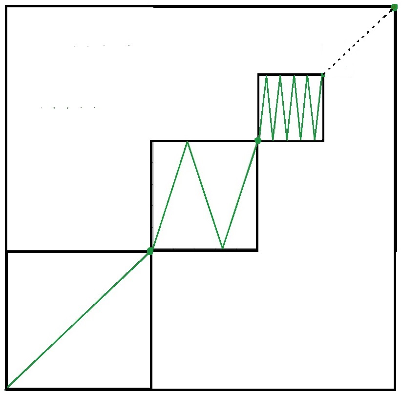
Example 1.3.
Let be given by and be the sequence whose general term is and For each , take the interval and let be the unique increasing affine map from onto . Let
(see Figure 1). It was shown in [23, Proposition 8] that and in [6, Example 10.3] that
In particular, the unique invariant probability measure maximizing (5) is the Dirac measure supported at and
1.2. Discontinuous maps
Another consequence of Theorem B is that, since it expresses the metric mean dimension of a map in terms of its induced subshift, we may regard one of the equalities in (3) as a definition of the metric mean dimension of an arbitrary (not necessarily continuous) map. The main difference from the continuous setting is that, for a discontinuous map , the transition set is no longer closed and therefore the sequence space induced by it is not a subshift. However, since the metric mean dimension does not distinguish a set from its closure (see Remark 2.2), it is natural to consider the subshift of compact type , which always satisfies
Definition 1.5.
Let be a compact metric space, be a (not necessarily continuous) map and . The upper/lower metric mean dimension of are given by
Let us see an interesting use of this definition. It is known (cf. [16, Proposition 15.2.13]) that if is a piecewise monotone map with finitely many, say , full branches, then
| (6) |
Our next result establishes an analogue formula for the metric mean dimension of piecewise monotone maps with infinitely many full branches. In this context, the role of counting branches (which represents the number of critical points of the map) is played by the computation of the box dimension of the (now infinite) set of critical points.
Let be a compact interval and be a compact set defined by , where are pairwise disjoint open intervals ordered non-increasingly in length such that . We note that the latter equality implies that has zero Lebesgue measure; and every compact subset of with zero Lebesgue measure has the previous structure. The intervals are referred to as the cut-out sets of and are deeply related to the box dimension of (cf. [9, Propositions 3.6 and 3.7]), which can be any value in .
Consider a map satisfying:
-
(C1)
is strictly monotone, for every .
-
(C2)
, for every .
-
(C3)
is differentiable and , for some and every
The next result relates the metric mean dimension of with the box dimension of , both with respect to the Euclidean distance . Regarding condition (C3), we refer the reader to Subsection 7.1.
Theorem C.
Let be a compact subset with zero Lebesgue measure and be any map satisfying conditions (C1)-(C3). Then
Moreover, if exists then
| (7) |
Example 1.6.
Example 1.7.
Regarding the two previous examples, it was proved in [19] that they belong in the class of EMR maps (cf [14, Definition 2.3]). It is also known that the pressure function associated to the parameterized geometric potential possesses a unique transition point
This value was computed explicitly in [14, Theorem 2.11], where it was shown to be equal to the box dimension of the corresponding set of discontinuities. By Theorem C we further conclude that, for these maps, is precisely the metric mean dimension with respect to the Euclidean distance. More precisely:
Corollary 1.8.
Assume that exists and that satisfies the additional condition
-
(C4)
Then
2. Preliminaries
Let be a compact metric space and be a continuous map.
2.1. Metric mean dimension
For each , define the Bowen metric
which is equivalent to . We sometimes refer to balls with respect to this metric as dynamical balls.
Given a subset of and , consider the following minimum
| (8) |
and the limit
which exists since the sequence is sub-additive in the variable . Recall that the topological entropy is given by
Definition 2.1.
The upper/lower metric mean dimension of are given, respectively, by
and
A subset is said to be separated with respect to the metric if for every ; it is spanning with respect to the metric if for every there exists some such that The notion of upper/lower metric mean dimension can be equivalently defined if one replaces by either
or
and replaces their limits in by either or
Remark 2.2.
Since for every and , the metric mean dimension does not distinguish a set from its closure. That is, for every ,
It is known that the metric mean dimension satisfies the following properties.
Proposition 2.3.
Let and be compact metric spaces and and be continuous maps.
If there exists a surjective Lipschitz map such that , then
Given a positive integer ,
2.2. Box dimension
Given , the upper and lower box dimension of is given by
As happens with the metric mean dimension, this notion may be equivalently defined using spanning/separated subsets of .
2.3. Katok entropy
Given an ergodic probability measure , , and , denote
where the infimum is taken over all measurable subsets with measure bigger than . In fact, the same value is attained if, instead of being just measurable, we assume that ranges over finite unions of dynamical balls whose union has measure bigger than We will always consider such s. The Katok entropy of at scale is given by
The following variational principle links Katok entropy and metric mean dimension (see [20] and [8]).
Theorem 2.4.
Let be a compact metric space and be a continuous map. Then, for every
For further use, we also include the following easy consequence of the previous variational principle.
Corollary 2.5.
Let be a compact metric space and be a continuous map. Then,
3. Proof of Theorem A
In this section we show that the unilateral and bilateral subshifts of compact type generated by a closed transition set have the same metric mean dimension. The next arguments hold for both upper and lower metric mean dimension, so to simplify the notation we will not distinguish them.
In what follows, or and, given a closed set , we consider the subshift of compact type
endowed with the distance
Denote and keep the notation and for the distance and dynamics restricted to , respectively. By Corollary 2.5, to prove Theorem A it is enough to show that
Firstly, note that the projection is Lipschitz, and . Hence, the restriction
satisfies the conditions in Proposition 2.3, and therefore
To show the reverse inequality we will make use of the variational principle provided by Theorem 2.4. Given a subshift , a finite set of coordinates and a collection of open subsets, the associated cylinder is defined by
| (9) |
These sets are generators of the topology of and every dynamical ball is a cylinder. Thus, for any ergodic measure , we can compute
by taking the infimum over finite unions of cylinders in whose union has measure bigger than . Note that, for every ergodic measure , its push-forward is ergodic. Moreover, every finite union of cylinders in with measure bigger than has as a pre-image by a finite union of cylinders with measure bigger than . Consequently,
| (10) |
We proceed by estimating the right hand side in (10). For each let be a positive integer such that and be any open cover of satisfying Given an open cover of a set such that , then
is an open cover of satisfying and . Thus, for every we have
Combining this information with (10) we get
Hence, for every ergodic probability measure we have
and therefore
Applying now Theorem 2.4, we obtain
and the proof of the proposition is complete. ∎
4. Proof of Theorem B
In this section we recall Friedland’s topologial entropy of a free semigroup action of continuous maps on a compact metric space X, which inspires a corresponding notion of metric mean dimension. Afterwards, we present the proposal in [5] for the metric mean dimension of a free semigroup action with respect to a fixed random walk. We proceed by establishing a variational principle connecting these concepts, from which Theorem B is a direct consequence.
4.1. Free semigroup actions
Let be a compact metric space and be a family of continuous maps. Denote by the free semigroup having as a generator, where the semigroup operation is the composition of maps. Let be the induced free semigroup action
Denoting the index set of by , we endow the product space with the metric
and consider the skew-product associated to the action :
where
4.1.1. Friedland’s approach
For a finite set of continuous maps , we consider the transition set
and the associated subshift of compact type
In what follows, the composition operation between two maps will be denoted by their concatenation.
Definition 4.1.
The Friedland topological entropy of with respect to is defined as
Actually, Friedland defined the entropy of as the infimum of over all finite sets of generators of . As both definitions that we consider are expressed in terms of a particular set of generators, we keep this dependence and omit from the notation. We now define the corresponding notion for the metric mean dimension.
Definition 4.2.
The upper/lower Friedland metric mean dimension of with respect to the set of generators is given by
| (11) |
By Theorem A, the above definition is independent of whether or Besides, it will be clear from Theorem 4.5 that the initial choice of the parameter to define the metric does not affect the value of the metric mean dimension. This is why on the left side of (11) we only write the metric used to generate The aim of Theorem B is to ensure that the above definition coincides with Lindenstrauss-Weiss’ one in the case when .
4.1.2. Carvalho, Rodrigues and Varandas’ approach
Now we present the definition of metric mean dimension introduced in [7]. This perspective is inspired by Bufetov (see [4]), where one selects randomly which element of will be used to evolve time on each step.
Following [7], we shall code different concatenations of elements in by distinct sequences of symbols. Even though an element of the group may be generated by different combinations of generators, we will simply consider different concatenations instead of the elements in the group they create, since we do not make use of the group structure.
For every and , consider the metric in given by
Fix a random walk, that is, a shift invariant Borel probability measure . The entropy of is given by
The topological entropy of with respect to the set of generators (cf. [7]) is given by
Definition 4.3.
The upper/lower metric mean dimension of with respect to the set of generators and the random walk are given, respectively, by
Once again, one can replace in the definition by either or as in Definition 2.1.
Definition 4.4.
Given a compact metric space , we say that is homogeneous if it is a fully supported doubling measure, namely,
Note that if a measure is homogeneous, then one can replace the factor on the radius of the balls by , up to changing the constant , which will then be denoted by . For instance, if a random walk is homogeneous, then
for every and , where
In what follows, we adopt the notation
4.1.3. Variational principle
Our main result in this section states that the two aforementioned notions of metric mean dimension of finitely generated free semigroup actions are equal. Theorem B corresponds to the particular case of .
Theorem 4.5.
Let be a compact metric space and be a collection of continuous maps in . Then,
| (12) | |||||
Moreover, the previous maxima are attained at every homogeneous random walk and we have
| (13) |
The equality (13) is a direct consequence of the fact that the maximum in (12) is attained by any fully supported Bernoulli measure - which is homogeneous - combined with [7, Corollary III]. In fact, the choice of metric in considered in [7] is different from our choice , but since both metrics are uniformly equivalent so are their products with and therefore their corresponding metric mean dimensions of the skew-product coincide.
Remark 4.6.
We observe that a statement analogous to Theorem 4.5 for the topological entropy of a semigroup action does not hold. Friedland showed [10, Lemma 3.6] that if is a non-involutive homeomorphism () of a compact metric space, then If we consider the phase space to be the unit circle, both and have zero topological entropy, and since compositions of them only represent delay in time, we have for every So
Actually, the Friedland subshift is a Lipschitz factor of the skew-product map - in particular, - and the entropy of the action relates to the one of the skew product by Bufetov’s formula (cf. [4]): if is the symmetric Bernoulli measure in the symbols of , then
Whereas, in the case of metric mean dimension, the normalization in its definition makes the second term in the right hand side vanish and we obtain (12) and (13).
Proof of Theorem 4.5.
We start by proving that the Friedland metric mean dimension is an upper bound for the one induced by any random walk. Let . For each consider a maximal separated subset with respect to the metric That is, for every we have
Let us denote simply . Then, the elements of
are separated. Hence, for every we have
Now let us show that the maximum is attained by any homogeneous . Take one such . Then, for every and , we have
Given and , let be a maximal separated subset in , that is, . Take such that By the Pigeonhole Principle, there exists a subset such that
-
•
all the transitions until the coordinate are given by the same tuple, which we denote by ;
-
•
Note that, by definition of , the property of being separated only depends on the first coordinates of the elements of . In particular, the first coordinate of all the elements in are necessarily different from each other. Reordering if necessary, we denote the elements of by
Then, the set is separated with respect to the metric for every In particular, the balls of radius with respect to centered at the elements of are pairwise disjoint. Hence,
for every . So,
Therefore,
We conclude after dividing by and making . ∎
4.2. Zero complexity maps may generate positive metric mean dimension
In this subsection we will make use of Theorem 4.5 to show that two maps with zero metric mean dimension may generate a free semigroup action with positive metric mean dimension. Let endowed with the Euclidean distance .
Proposition 4.7.
There exist two zero entropy continuous maps satisfying
In particular, the topological entropy of the action is infinite.
Proof.
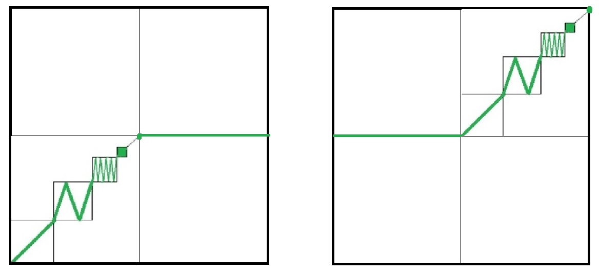
Let be the map defined in Example 1.3. We consider the maps
The transition set which generates the Friedland subshift is illustrated in Figure 2.
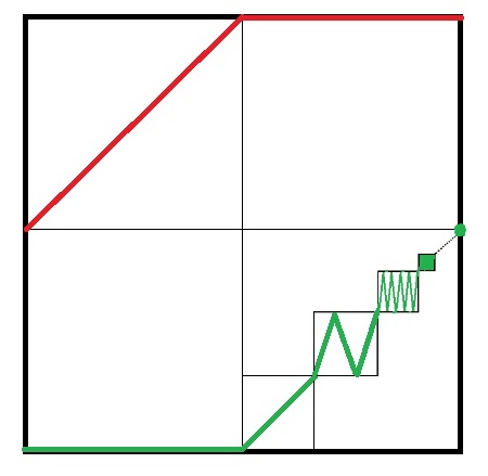
Since and , it is clear that their topological entropy is zero, and so both maps have zero metric mean dimension. We also observe that - denoting the Bowen metric of time with respect to a map by - we have (see Figure 3)
In order to prove the lower bound
we consider the random walk Fix (the case is analogous). Since
we have
and so
which implies that
Fix Since , every must be prescribed by the same transitions as , namely, there exists such that for every and . Let us estimate separately for each type of .
Case 1:
Let be such that . Then we have for every and . Then,
| (15) |
Case 2:
.
In this case, . Given , we have two possibilities
-
•
If , then This implies that and for every Then, .
-
•
If , then and This implies that and for every Hence,
Thus,
which implies that
.
Take such that , assuming without loss that is even. Given , we have for every . If , we get , since the separation between and must occur between the coordinates and and we may restrict to even times. In particular, this implies that
Hence
Bringing together sub-cases and we conclude that for every such that one has
| (16) |
Case 3:
Since is a homeomorphism, and , we have
| (17) |
where the inequality follows from Case 2. Combining (14), (15),(16) and (4.2) we deduce that
This finishes the proof of Proposition 4.7. ∎
Proposition 4.7 seems optimal. If two maps have zero complexity (in terms of metric mean dimension) but the associated action does not, the richness of the orbit structure can only be revealed after a composition of the two maps. This indicates that we need twice the time to see this maximal value, which is always bounded by the dimension of the phase space. This motivates the following
Question 1.
Let be a compact metric space and be continuous maps with zero metric mean dimension. Is it true that
5. Proof of Corollary 1.1
Recall that, given and ,
Let be such that every satisfies
which always exists by [6, Theorem E]. Fix one such Then, for any , we have
where Given , let be a positive integer satisfying For , consider a maximal separated subset Then, there exist such that
-
•
, for every and
-
•
Hence
and so
where the last equality is due to Theorem B. On the other hand, by definition, the reverse inequality always holds. Hence,
Now, since is invariant, we may carry on the same reasoning with replaced by , obtaining
| (18) |
Let us consider the empirical measures along the orbit of . For each , denote , which by (18) satisfies . Due to the upper-semicontinuity of , any weak* limit of is invariant and satisfies
In general, the previous maximizing measure is not ergodic. Yet, as is affine, the maximum in Corollary 1.1 is also attained at some ergodic probability measure.
Finally, observe that given any measure satisfying
since , there exists a full measure set such that Therefore, since and is upper semi-continuous, we deduce that ∎
6. Spectral radius bounds for subshifts of compact type
In what follows, we recall from [10] an upper bound for the entropy of subshifts of compact type in terms of the spectral radius of a suitable matrix. Fix a compact metric space and a subset
Given , let be an open cover of Consider the matrix given by
By counting arguments similar to the ones used for subshifts of finite type, we know that many cylinders composed by elements of of size are enough to cover , where denotes the sum norm in the space of matrices. This estimate yields the following equivalent formulation of [10, Lemma 4.1], where stands for the spectral radius of the matrix .
Lemma 6.1.
Let be a compact metric space and . Then
In the case (and also in higher dimensions), the matrix can be replaced by another one constructed by using intersections with an grid instead of an open cover. More precisely, given and , we define
| (19) |
In the remaining of this paper the notation will always refer to (19), for which we have the following reformulation of Lemma 6.1.
Lemma 6.2.
Let be the Euclidean distance in and . Then
The previous lemmas will be very useful tools to estimate the metric mean dimension when combined with the following property of complex matrices.
Theorem 6.3 (Gershgorin Circle Theorem, [11]).
Let be a complex matrix. Then, every eigenvalue of is contained in the union
where and for every
In particular, if we apply Theorem 6.3 to a matrix and its transpose, we get
| (20) |
In the following example we will apply the estimates above to compute the metric mean dimension on a class of subshifts of compact type.
6.1. Delayed full shifts
Let us consider a family of maps which are prescribed by a closed set and a collection of finite transitions which connect any pair of points in the set. We will use the information of the previous subsection with a slight modification: the only difference in the method is that we code different elements of the cover by the same symbol as long as they behave in a similar manner.
Proposition 6.4.
Let be a compact metric space. Fix a positive integer and select distinct points and a closed subset . Consider given by
Then,
Proof.
The computations below do not depend on whether we take upper or lower limits in , so we do not distinguish them by the notation. We will denote the metric defined in (1) by .
For the converse inequality, we may assume without loss of generality that for every . Otherwise, the set would be contained in corresponding to , whose upper and lower box dimension are equal to the ones of
Given we consider a minimal open cover of , that is, . We can assume that uniquely. For each , consider the following open cover of by cylinders (see (9))
In order to estimate the cardinality of , we partition its elements in the following way: for each , let
Note that
or equivalently,
We denote the above equality by , where and . Then,
Let be a positive integer satisfying . Then and we get
| (21) |
On the other hand, it is easy to see that the entries of are polynomials in of degree at most . Consequently, there exists independent of satisfying . Combining this information with (21) we obtain
We finish the proof by dividing by and making . ∎
7. Proof of Theorem C
In this section we fix a compact interval , a compact subset with zero Lebesgue measure and the associated family of cut-out sets , ordered non-increasingly in diameter. For each , let and denote the Euclidean distance in by . From now on we will assume that for every If, otherwise, there is such that , then has finitely many branches and so, by (6), its entropy is finite; therefore its metric mean dimension is zero, trivially satisfying (7).
For the sets under consideration, the following dimension estimates via cut-out sets are provided by [9, Propositions 3.6 and 3.7].
Lemma 7.1.
Let and be as above. Then
Moreover, the box dimension of exists if, and only if, the outer limits coincide.
Theorem C is a consequence of the previous lemma together with the following inequalities, which are the content of Propositions 7.2 and 7.3:
To prove the following proposition, the differentiability assumption (C3) in the statement of the theorem is not needed.
Proposition 7.2.
Let be a map satisfying conditions (C1) and (C2). Then
Proof.
By Definition 1.5 of metric mean dimension, we must consider and the subset endowed with the metric
Given , each bijectivity domain have length at least Let be a reordering of so that are ordered from left to right. Then the sets are pairwise separated by at least Since condition (C2) ensures that each cylinder composed by is nonempty, for every
This implies that
Thus,
Given , take satisfying Thus,
We finish the proof by making (and consequently ). ∎
Proposition 7.3.
Let be a map satisfying conditions (C1)-(C3). Then
Proof.
Assume for simplicity that and fix . By Lemma 6.2 and (6) we have
| (22) |
where is defined as in (19). For each fix any point and observe that is a sequence that intersects each exactly once, by conditions (C1) and (C2).
Let be a positive integer such that , where is as in (C3). The graph of can never intersect more than boxes in the grid per line. Otherwise, by the Mean Value Theorem there would exist some point in the interior of such that Hence, for every we have
| (23) |
where the second inequality is due to the fact that every open interval of diameter can intersect at most intervals of the form , and the last inequality is a consequence of the next lemma.
Lemma 7.4.
Let be a sequence of positive real numbers such that , for every . Then for every ,
Proof.
Given a minimal collection of intervals of diameter at most that covers , there can be at most one element of in between each pair of consecutive intervals not yet covered. Adding one extra interval for each of these (at most ) points, we get an cover of with cardinality . ∎
7.1. Large derivative assumption
Condition (C3) was used in the previous reasoning to obtain a uniform upper bound for the number of entries equal to in every row of in terms of the covering number of . However, it is not strictly necessary as we will illustrate.
Example 7.5.
Let us compute the metric mean dimension, with respect to the Euclidean distance , of the following (discontinuous) interval map
We start by observing that the map does not satisfy either of the conditions (C2) (since restricted to the left and rightmost intervals is not full branch) and (C3) (since there are infinitely many differentiable maxima and minima). In order to show that (C3) is not strictly necessary for Theorem C to be valid, we must consider a map satisfying (C2). After computing the metric mean dimension of , we will consider a slightly modified map satisfying (C2) and such that all the estimates still hold.
The map can be seen as satisfying condition (C1) and, up to the left and rightmost intervals, also (C2), where Let us prove that
| (24) |
Firstly, an argument similar to the one in the proof of Proposition 7.2 yields
For the converse inequality, we cannot directly apply Proposition 7.3 since the map does not satisfy (C3). The main idea is still to make use of Lemma 6.2 and (6). However, we will estimate the number of ’s in a column by making use of the Second Order Mean Value Theorem.111 If is twice differentiable, then for some
For each , fix the scale and consider an grid. To estimate the spectral radius of - defined in (19) - we restrict our attention to the first quadrant, as the remaining ones can be dealt in an analogous way.
Consider the positive maximum points , . Given and such that , which implies , we have two possibilities:
-
(i)
Let be such that . Then,
Thus, if is close enough to .
-
(ii)
Thus, if is close enough to .
From now on, we fix close enough to so that the two previous estimates hold. Take big enough so that . Let us bound the spectral radius of from above by estimating the number of ’s. To do so, we recall from (6) that
and separate in classes. First, note that for every . This implies that every interval , , contains at least two ’s. Therefore,
| (25) |
Case 1: .
For each , consider the nearest points such that . Then
By the Second Order Mean Value Theorem, for every there exists such that . Moreover, by the choice of we have and , for every . Combining this information with (25), we obtain
| (26) |
where is a constant independent of .
Case 2:
For each , consider the nearest points such that and . Then
By the Second Order Mean Value Theorem, for every and there exists such that . Again, by the choice of we have and , for every . Joining this information with (25), we obtain
| (27) |
for every where is a constant independent of .
Case 3:
By taking large enough, we may assume that . Thus, , for every such that for some . Hence, there exists some such that, for every such , we have
By the proof of Proposition 7.3 we obtain
| (28) |
for every .
Bringing together (7.5), (7.5) and (28), and proceeding analogously in the other quadrants, we conclude that there exists a constant , which depends only on , such that
for every large enough .
We are ready to complete the computation of the upper bound of the metric mean dimension of . Given , take such that . Then
and so
We finish this section by observing that all arguments used to compute the metric mean dimension of the map remain valid if we consider a smooth perturbation of in small neighbourhoods and , so that and for every . In this case, we obtain a map satisfying (C1) and (C2) such that the equality (7) in Theorem C still holds, even though the assumption (C3) does not.
7.2. A remark on the definition of metric mean dimension of discontinuous maps
Given a discontinuous map , its associated transition set is not closed. In order to associate a subshift of compact type to , we could have followed two possible paths: one option would be to take the closure of the transition set and afterwards consider its associated sequence space ; another way (which is the one we chose) is to consider the closure of the sequence space . At first glance, the former might appear more satisfactory since, by Theorem A, we would obtain a notion of metric mean dimension that could be expressed both by unilateral and bilateral sequences. Let us exemplify why it would not yield a meaningful notion of metric mean dimension.
Consider the set and let be any map satisfying conditions (C1)-(C3). The arguments in the proof of Theorem C do not depend whether we define in terms of or . This indicates that
| (29) |
is the right value for it. Yet, if we consider an interval map such that and , then any meaningful notion of metric mean dimension compatible with (29) should also be zero. However, since we have
then Proposition 6.4 implies that
This shows that taking the closure of the transition set prior to generating the sequences may create too many new orbits that are not present in the original dynamics.
Acknowledgments
This work commenced during the author’s Master’s degree program at Universidade Federal do Rio Grande do Sul, Brazil, under the supervision of Professor Alexandre Baraviera, to whom he is deeply grateful. The author also thanks Professor Paulo Varandas for the insightful conversations and Professor Maria Carvalho for the meticulous reading and numerous suggestions that significantly improved this manuscript. The author has been awarded a PhD grant by FCT- Fundação para a Ciência e a Tecnologia, with reference UI/BD/152212/2021.
References
- [1] J. F. Alves. Nonuniformly Hyperbolic Attractors Geometric and Probabilistic Aspects. Springer Monographs in Mathematics, 2020.
- [2] R. Bowen. Topological entropy and axiom A. Proceedings of Symposia in Pure Mathematics, American Mathematical Society, Providence, RI, 1970, 23–41.
- [3] D. Burguet, R. Shi. Mean dimension of continuous cellular automata. Israel J. Math. 259 (2024) 311–346.
- [4] A. Bufetov. Topological entropy of free semigroup actions and skew-product transformations. J. Dyn. Control Syst. 5 (1999) 137–143.
- [5] M. Carvalho, F. B. Rodrigues and P. Varandas. A variational principle for free semigroup actions. Adv. Math. 334 (2018) 450–487.
- [6] M. Carvalho, G. Pessil and P. Varandas. A convex analysis approach to the metric mean dimension: limits of scaled pressures and variational principles. Adv. Math. 436 (2024) 109407
- [7] M. Carvalho, F. Rodrigues and P. Varandas. A variational formula for the metric mean dimension of free semigroup actions. Ergodic Theory Dynam. Systems 42 (2021) 65–85.
- [8] D. Cheng and Z. Li. Scaled pressure of dynamical systems. J. Differential Equations 342 (2023) 441–471.
- [9] K. Falconer. Techniques in Fractal Geometry. Wiley, 1997.
- [10] S. Friedland. Entropy of graphs, semigroups and groups. Ergodic Theory of -Actions, London Math. Soc. Lecture Notes Ser. 228, Cambridge Univ. Press, 1996, pp. 319–343.
- [11] S. Gerschgorin. Über die Abgrenzung der Eigenwerte einer Matrix. Izv. Akad. Nauk. 6 (1931) 749–754.
- [12] Y. Gutman and A. Śpiewak. Metric mean dimension and analog compression. IEEE Trans. Inform. Theory 66:11 (2020) 6977–6998.
- [13] Y. Gutman and M. Tsukamoto. Embedding minimal dynamical systems into Hilbert cubes. Invent. Math. 211 (2020) 113–166.
- [14] G. Iommi and A. Velozo. Pressure, Poincaré series and box dimension of the boundary. Nonlinearity 34 (2021) 3936–3952
- [15] A. Katok. Lyapunov exponents, entropy and periodic orbits for diffeomorphisms. Publ. Math. Inst. Hautes Études Sci. 51 (1980) 137–173.
- [16] A. Katok and B. Hasselblat. Introduction to the Modern Theory of Dynamical Systems. Encyclopedia of Mathematics and its Applications, vol 54. Cambridge University Press, 1995.
- [17] E. Lindenstrauss and B. Weiss. Mean topological dimension. Israel J. Math. 115 (2000) 1–24.
- [18] G. Pessil. Dimensão Métrica Média de Deslocamentos de Tipo Finito em Alfabetos Compactos. Master Thesis (in Portuguese), Universidade Federal do Rio Grande do Sul - UFRGS, Brazil, 2021.
- [19] M Pollicott and H. Weiss. Multifractal analysis of Lyapunov exponent for continued fraction and Manneville–Pomeau transformations and applications to diophantine approximation. Commun. Math. Phys. 207 (1999) 145–171
- [20] R. Shi. On variational principles for metric mean dimension. IEEE Trans. Inform. Theory 68:7 (2022) 4282–4288.
- [21] M. Tsukamoto. Remark on the local nature of metric mean dimension. Kyushu Journal of Mathematics 76:1 (2022) 143–162.
- [22] M. Tsukamoto. Mean dimension of full shifts. Israel J. Math. 230 (2019) 183–193.
- [23] A. Velozo and R. Velozo. Rate distortion theory, metric mean dimension and measure theoretic entropy. Preprint, 2017, arXiv:1707.05762