Probabilistic learning rate scheduler with provable convergence

Abstract

Learning rate schedulers have shown great success in speeding up the convergence of learning algorithms in practice. However, their convergence to a minimum has not been proven theoretically. This difficulty mainly arises from the fact that, while traditional convergence analysis prescribes to monotonically decreasing (or constant) learning rates, schedulers opt for rates that often increase and decrease through the training epochs. In this work, we aim to bridge the gap by proposing a probabilistic learning rate scheduler (PLRS), that does not conform to the monotonically decreasing condition, with provable convergence guarantees. In addition to providing detailed convergence proofs, we also show experimental results where the proposed PLRS performs competitively as other state-of-the-art learning rate schedulers across a variety of datasets and architectures.

Keywords: learning rate schedulers, stochastic gradient descent, convergence analysis, saddle points, non-convex optimization

I Introduction

Over the last two decades, there has been increased interest in analyzing the convergence of gradient descent-based algorithms. This can be majorly attributed to their extensive use in the training of neural networks and their numerous derivatives. Stochastic Gradient Descent (SGD) and their adaptive variants such as Adagrad [1], Adadelta [2], and Adam [3] have been the choice of optimization algorithms for most machine learning practitioners, primarily due to their ability to process enormous amounts of data in batches. Even with the introduction of adaptive optimization techniques that use a default learning rate, the use of stochastic gradient descent with a tuned learning rate was quite prevalent, mainly owing its generalization properties [4]. However, tuning the learning rate of the network can be computationally intensive and time consuming.
     Various methods to efficiently choose the learning rate without excessive tuning have been explored. One of the initial successes in this domain is the random search method [5]; here, a learning rate is randomly selected from a specified interval across multiple trials, and the best performing learning rate is ultimately chosen. Following this, more advanced methods such as Sequential Model-Based Optimization (SMBO) [6] for the choice of learning rate became prevalent in practice. SMBO represents a significant advancement over random search by tracking the effectiveness of learning rates from previous trials and using this information to build a model that suggests the next optimal learning rate. A tuning method for shallow neural networks based on theoretical computation of the Hessian Lipschitz constant was proposed by [7].

Several works on training deep neural networks prescribed the use of a decaying learning rate scheduler [8, 9, 10]. Recently, much attention has been paid to cyclically varying learning rates [11]. By varying learning rates in a triangular schedule within a predetermined range of values, the authors hypothesize that the optimal learning rate lies within the chosen range, and the periodic high learning rate helps escape saddle points. Although no theoretical backing has been provided, it was shown to be a valid hypothesis owing to the presence of many saddle points in a typical high dimensional learning task [12]. Many variants of the cyclic learning rate schedule have henceforth been used in various machine learning tasks [13, 14, 15]. A cosine-based cyclic learning rate schedule proposed by [16] has also found several applications, including Transformers [17, 18]. Following the success of the cyclic learning rate schedulers, a one-cycle learning rate scheduler proposed by [19] has been observed to provide faster convergence empirically; this was attributed to the injection of ‘good noise’ by higher learning rates which helps in convergence. Although empirical validation and intuitions were provided to support the working of these learning rate schedulers, a theoretical convergence guarantee has not been provided to the best of our knowledge.

Another line of research that is closely aligned with our work in terms of the analysis framework is the convergence analysis of perturbed gradient descent and stochastic gradient descent methods. In [20], the vanilla gradient descent is perturbed by samples from a ball whose radius is fixed using the optimization function-specific constants. They show escape from a saddle point by characterizing the distribution around a perturbed iterate as uniformly distributed over a perturbation ball along which the region corresponding to being stuck at a saddle point is shown to be very small. In [21], the saddle point escape for a perturbed stochastic gradient descent is proved using the second-order Taylor approximation of the optimization function, where the perturbation is applied from a unit ball to the stochastic gradient descent update.

I-A Motivation

Traditional convergence analysis of gradient descent algorithms and its variants requires the use of a constant or a decaying learning rate [22]. However, with the introduction of learning rate schedulers, the learning rates are no longer monotonically decreasing. Rather, their values heavily fluctuate, with the occasional use of very large learning rates. Although there are ample justifications provided for the success of such methods, there are no theoretical results which prove that stochastic gradient descent algorithms with fluctuating learning rates converge to a local minimum in a non-convex setting. With the increase of emphasis on trustworthy artificial intelligence, we believe that it is important to no longer treat optimization algorithms as black-box models, and instead provide provable convergence guarantees while deviating from the proven classical implementation of the descent algorithms. In this work, we aim to bridge the gap by providing rigorous mathematical proof for the convergence of our proposed probabilistic learning rate scheduler with SGD.

I-B Our contributions

1. We propose a new Probabilistic Learning Rate Scheduler (PLRS) where we model the learning rate as an instance of a random noise distribution.

2. We provide convergence proofs to show that SGD with our proposed PLRS converges to a local minimum in Section IV. To the best of our knowledge, we are the first to theoretically prove convergence of SGD with a learning rate scheduler that does not conform to constant or monotonically decreasing rates. Our main contribution is in showing how our learning rate scheduler, in combination with inherent SGD noise, speeds up convergence by escaping saddle points.

3. Our proposed probabilistic learning rate scheduler, while being provably convergent, can be seamlessly ported into practice without the knowledge of theoretical constants (like gradient and Hessian Lipschitz constants). We illustrate the efficacy of the PLRS through extensive experimental validation, where we compare the accuracies with state-of-the-art schedulers in Section V. We show that the proposed method outperforms popular schedulers such as cosine annealing [16], one-cycle [19], knee [23] and the multi-step scheduler when used with ResNet-110 on CIFAR-100, VGG-16 on CIFAR-10 and ResNet-50 on Tiny ImageNet, while displaying comparable performances on other architectures like DenseNet-40-12 and WRN-28-10 when trained on CIFAR-10 and CIFAR-100 datasets respectively. We provide our base code with all the hyper-parameters for reproducibility.

II Probabilistic learning rate scheduler

Let $f:\mathbb{R}^{d}\rightarrow\mathbb{R}$ be the function to be minimized. The unconstrained optimization, $\min_{\textbf{x}\in\mathbb{R}^{d}}f(\bf x)$, can be solved iteratively using stochastic gradient descent whose update equation at time step $t$ is given by

$$\mathbf{x}_{t+1}=\mathbf{x}_{t}-\eta_{t}g(\mathbf{x}_{t}).$$

Here, $\eta_{t}\in\mathbb{R}$ is the learning rate and $g(\mathbf{x}_{t})$ is the stochastic gradient of $f(\bf x)$ at time $t$. In this work, we propose a new learning rate scheduler, in which the learning rate $\eta_{t}$ is sampled from a uniform random variable,

$$\eta_{t}\sim\mathcal{U}[L_{min},L_{max}],\quad 0<L_{min}<L_{max}<1.$$

Note that contrary to existing learning rate schedulers, which are deterministic functions, we propose that the learning rate at each time instant $t$ be a realization of a uniformly distributed random variable. Although the learning rate in our method is not scheduled, but is rather chosen as a random sample at every time step, we call our proposed method Probabilistic Learning Rate Scheduler to keep in tune with the body of literature on learning rate schedulers.

In order to represent our method in the conventional form of the stochastic gradient descent update, we split the learning rate $\eta_{t}$ into a constant learning rate $\eta_{c}$ and a random component, as $\eta_{t}=\eta_{c}+u_{t}$, where $u_{t}\sim\mathcal{U}[L_{min}-\eta_{c},L_{max}-\eta_{c}]$. The stochastic gradient descent update using the proposed PLRS (referred to as SGD-PLRS) takes the form

$$\mathbf{x}_{t+1}=\mathbf{x}_{t}-(\eta_{c}+u_{t+1})g(\mathbf{x}_{t})=\mathbf{x}_{t}-\eta_{c}\nabla f(\mathbf{x}_{t})-\mathbf{w}_{t},$$ (1)

where we define $\mathbf{w}_{t}$ as

$$\mathbf{w}_{t}=\eta_{c}g(\mathbf{x}_{t})-\eta_{c}\nabla f(\mathbf{x}_{t})+u_{t+1}g(\mathbf{x}_{t}).$$ (2)

Here, $\nabla f(\mathbf{x}_{t})$ refers to the true gradient, i.e., $\nabla f(\mathbf{x}_{t})=\mathbb{E}[g(\mathbf{x}_{t})]$. Note that in (1), the term $\mathbf{x}_{t}-\eta_{c}\nabla f(\mathbf{x}_{t})$ resembles the vanilla gradient descent update and $\mathbf{w}_{t}$ encompasses the noise in the update; the noise is inclusive of both the randomness due to the stochastic gradient as well as the randomness from the proposed learning rate scheduler. We set $\eta_{c}=\frac{L_{min}+L_{max}}{2}$ so that the noise $\mathbf{w}_{t}$ is zero mean, which we prove later in Lemma 1.

Remark 1.

It is interesting to note that a periodic learning rate scheduler such as triangular, or cosine annealing based scheduler can be considered as a single instance of our proposed PLRS. The range of values assigned to the learning rate $\eta_{t}$ is pre-determined in both cases. In fact, for any learning rate scheduler, the basic mechanism is to vary the learning rate between a low and a high value - the high learning rates help escape the saddle point by perturbing the iterate, whereas the low values help in convergence. This pattern of switching between high and low values can be achieved through both stochastic and deterministic mechanisms. While the current literature explores the deterministic route (without providing analysis), we propose and explore the stochastic variant here and also provide a detailed analysis.

III Preliminaries and definitions

Definition 1.

A function $f:\mathbb{R}^{d}\rightarrow\mathbb{R}$ is said to be $\beta$-smooth (also referred to as $\beta$-gradient Lipschitz) if, for $\beta\geq 0$,

$$\left\lVert\nabla f(\mathbf{x})-\nabla f(\mathbf{y})\right\rVert\leq\beta\left\lVert\mathbf{x}-\mathbf{y}\right\rVert,\quad\forall\mathbf{x},\mathbf{y}\in\mathbb{R}^{d}.$$

Definition 2.

A function $f:\mathbb{R}^{d}\rightarrow\mathbb{R}$ is said to be $\rho$-Hessian Lipschitz if for $\rho\geq 0$,

$$\left\lVert\textbf{H}(\textbf{x})-\textbf{H}(\textbf{y})\right\rVert\leq\rho\left\lVert\mathbf{x}-\mathbf{y}\right\rVert,\quad\forall\mathbf{x},\mathbf{y}\in\mathbb{R}^{d}.$$

Informally, a function is said to be gradient/Hessian Lipschitz, if the rate of change of the gradient/Hessian with respect to its input is bounded by a constant, i.e., the gradient/Hessian will not change rapidly. We now proceed to define approximate first and second-order stationary points of a given function $f$.

Definition 3.

For a function $f:\mathbb{R}^{d}\rightarrow\mathbb{R}$ that is differentiable, we say $\mathbf{x}\in\mathbb{R}^{d}$ is an $\epsilon$- first-order stationary point ($\epsilon$-FOSP), if for a small positive value of $\epsilon$, $\left\lVert\nabla f(\mathbf{x})\right\rVert\leq\epsilon.$

Before we define an $\epsilon$-second order stationary point, we define a saddle point.

Definition 4.

For a $\rho$-Hessian Lipschitz function $f:\mathbb{R}^{d}\rightarrow\mathbb{R}$ that is twice differentiable, we say $\textbf{x}\in\mathbb{R}^{d}$ is a saddle point if,

$$\left\lVert\nabla f(\mathbf{x})\right\rVert\leq\epsilon\quad\text{and}\quad\lambda_{min}(\textbf{H}(\textbf{x}))\leq-\sqrt{\rho\epsilon}.$$

For a convex function, it is sufficient if the algorithm is shown to converge to the $\epsilon$-FOSP as it would be the global minimum. However, in the case of a non-convex function, a point satisfying the condition for an $\epsilon$-FOSP may not necessarily be a local minimum, but could be a saddle point or a local maximum. Hence, the Hessian of the function is required to classify it as a second-order stationary point, as defined below. Note that, in our analysis, we prove convergence of SGD-PLRS to the approximate second-order stationary point.

Definition 5.

For a $\rho$-Hessian Lipschitz function $f:\mathbb{R}^{d}\rightarrow\mathbb{R}$ that is twice differentiable, we say $\mathbf{x}\in\mathbb{R}^{d}$ is an $\epsilon$-second-order stationary point ($\epsilon$-SOSP) if,

$$\left\lVert\nabla f(\mathbf{x})\right\rVert\leq\epsilon\quad\text{and}\quad\lambda_{min}(\textbf{H}(\textbf{x}))\geq-\sqrt{\rho\epsilon}.$$

Definition 6.

A function $f:\mathbb{R}^{d}\rightarrow\mathbb{R}$ is said to possess the strict saddle property at all $\textbf{x}\in\mathbb{R}^{d}$ if x fulfills any one of the following conditions: (i) $\left\lVert\nabla f(\mathbf{x})\right\rVert\geq\epsilon$, (ii) $\lambda_{min}(\textbf{H}(\textbf{x}))\leq-\sqrt{\rho\epsilon},$ (iii) $\mathbf{x}$ is close to a local minimum.

The strict saddle property ensures that an iterate stuck at a saddle point has a direction of escape.

Definition 7.

A function $f:\mathbb{R}^{d}\rightarrow\mathbb{R}$ is $\alpha-$strongly convex if $\lambda_{min}(\textbf{H}(\textbf{x}))\geq\alpha\quad\forall\mathbf{x}\in\mathbb{R}^{d}$.

We now provide the formal definitions of two common terms in time complexity.

Definition 8.

A function $f(s)$ is said to be $O(g(s))$ if $\exists$ a constant $c>0$ such that $|f(s)|\leq c|g(s)|$. Here $s\in S$ which is the domain of the functions $f$ and $g$.

Definition 9.

A function $f(s)$ is said to be $\Omega(g(s))$ if $\exists$ a constant $c>0$ such that $|f(s)|\geq c|g(s)|$.

In our analysis, we introduce the notations $\tilde{O}(.)$ and $\tilde{\Omega}(.)$ which hide all factors (including $\beta$, $\rho$, $d$, and $\alpha$) except $\eta_{c}$, $L_{min}$ and $L_{max}$ in $O$ and $\Omega$ respectively.

IV Proof of convergence

In this section, we present our convergence proofs to theoretically show that the proposed PLRS method converges to an $\epsilon$-SOSP in finite time. We first state the assumptions that are instrumental for our proofs. Note that these assumptions are similar to those in literature [21, 20, 24].

Assumptions.

• The function $f$ is $\beta$-smooth.

• The function $f$ is $\rho$-Hessian Lipschitz.

• The norm of the stochastic gradient noise is bounded i.e, $\left\lVert g(\mathbf{x}_{t})-\nabla f(\mathbf{x}_{t})\right\rVert\leq Q\quad\forall t\geq 0$. Further, $\mathbb{E}[Q^{2}]\leq\sigma^{2}$.

• The function $f$ has strict saddle property.

• The function $f$ is bounded i.e., $|f(\mathbf{x})|\leq B,\;\forall\mathbf{x}\in\mathbb{R}^{d}$.

• The function $f$ is locally $\alpha-$strongly convex i.e, in the $\delta$-neighborhood of a locally optimal point $\mathbf{x}^{*}$ for some $\delta>0$.

Remark 2.

If $\nabla\tilde{f}(\tilde{\mathbf{x}}_{t})$ and $\tilde{g}(\tilde{\mathbf{x}}_{t})$ are the gradient and stochastic gradient of the second order Taylor approximation of $f$ about the iterate $\tilde{\mathbf{x}}_{t}$, from Assumption A3, it is implied that $\left\lVert\tilde{g}(\tilde{\mathbf{x}}_{t})-\nabla\tilde{f}(\tilde{\mathbf{x}}_{t})\right\rVert\leq\tilde{Q}$. Further, $\mathbb{E}[\tilde{Q}^{2}]\leq\tilde{\sigma}^{2}$.

Before presenting the proofs, we reiterate the update equations of the proposed SGD-PLRS.

$$\mathbf{x}_{t+1}=\mathbf{x}_{t}-\eta_{c}\nabla f(\mathbf{x}_{t})-\mathbf{w}_{t}.$$ (1)

$$\mathbf{w}_{t}=\eta_{c}g(\mathbf{x}_{t})-\eta_{c}\nabla f(\mathbf{x}_{t})+u_{t+1}g(\mathbf{x}_{t}).$$ (2)

The proof structure presented in this section is inspired by the convergence analysis provided for the noisy gradient descent algorithm proposed for escaping saddle points in the work by [21]. Note that, (1) varies from the update equation analyzed by [21] due to the distinct characterization of the noise term in (2). Although the update may look similar to other perturbed gradient methods [20, 21, 24], we call attention to two significant differences: (i) In contrast to the isotropic additive perturbation commonly added to the SGD update, we introduce randomness in our learning rate which manifests as multiplicative noise in the update. This makes the characterization of the total noise dependent on the gradient, making the analysis challenging. (ii) The magnitude of noise injected is computed through the smoothness constants in the work by [20, 24]; instead, we treat the parameters $L_{min}$ and $L_{max}$ as hyperparameters to be tuned. This enables our PLRS method to be easily applied to training deep neural networks where the computation of these smoothness constants could be infeasible due to sheer computational complexity. We begin our proof discussion by noting that the term $\textbf{w}_{t}$ has zero mean and state this formally in the lemma below.

Lemma 1 (Zero mean property).

The mean of $\mathbf{w}_{t-1}\;\forall t\geq 1$ is $0$.

Proof.

$$\mathbb{E}[\mathbf{w}_{t-1}] =\mathbb{E}\left[\eta_{c}g(\mathbf{x}_{t-1})-\eta_{c}\nabla f(\mathbf{x}_{t-1})\right]+\mathbb{E}\left[u_{t}g(\mathbf{x}_{t-1})\right]$$

$$=\mathbf{0}\qquad\forall t\geq 1.$$

This follows as $\mathbb{E}[u_{t}]=\frac{L_{min}+L_{max}-2\eta_{c}}{2}=0$ and $\mathbb{E}\left[g(\mathbf{x}_{t-1})\right]=\nabla f(\mathbf{x}_{t-1})$. ∎

For a function satisfying the Assumptions A1-A6, there are three possibilities for the iterate $\textbf{x}_{t}$ with respect to the function’s gradient and Hessian.

• Gradient is large: $\left\lVert\nabla f(\mathbf{x}_{t})\right\rVert\geq\epsilon$.

• Gradient is small; iterate is around a saddle point: $\left\lVert\nabla f(\mathbf{x}_{t})\right\rVert\leq\epsilon,\lambda_{min}(\textbf{H}(\mathbf{x}_{t}))\leq-\gamma$.

• Gradient is small; iterate is around the $\epsilon$-SOSP: $\left\lVert\nabla f(\mathbf{x}_{t})\right\rVert\leq\epsilon,\lambda_{min}(\textbf{H}(\mathbf{x}_{t}))\geq-\gamma$.

Here $\epsilon,\gamma>0$. We now present three theorems corresponding to each of these cases.

Our first result pertains to the case B1 where the gradient of the iterate is large.

Theorem 1.

Under the assumptions A1 and A3 with $L_{max}<\frac{1}{\beta}$, for any point $\mathbf{x}_{t}$ with $\left\lVert\nabla f(\mathbf{x}_{t})\right\rVert\geq\sqrt{3\eta_{c}\beta\sigma^{2}}$ where $\sqrt{3\eta_{c}\beta\sigma^{2}}<\epsilon$, after one iteration, we have

$$\mathbb{E}[f(\mathbf{x}_{t+1})]-f(\mathbf{x}_{t})\leq-\tilde{\Omega}(L_{max}^{2}).$$

This theorem suggests that, for any iterate $\mathbf{x}_{t}$ for which the gradient is large, the expected functional value of the subsequent iterate $f(\mathbf{x}_{t+1})$ decreases, and the corresponding decrease $\mathbb{E}[f(\mathbf{x}_{t+1})]-f(\mathbf{x}_{t})$ is in the order of $\tilde{\Omega}(L_{max}^{2})$. The formal proof for this theorem can be found in Appendix A.

The next theorem corresponds to the case B2 where the gradient is small and the Hessian is negative.

Theorem 2.

Consider $f$ satisfying Assumptions A1 - A5. Let $\{\textbf{x}_{t}\}$ be the SGD iterates of the function $f$ using PLRS. Let $\left\lVert\nabla f(\textbf{x}_{0})\right\rVert\leq\epsilon$ and $\lambda_{min}(\textbf{H}(\textbf{x}_{0}))\leq-\gamma$ where $\epsilon,\gamma>0$. Then, there exists a $T=\tilde{O}\left(L_{max}^{-1/4}\right)$ such that with probability at least $1-\tilde{O}\left(L_{max}^{7/2}\right)$,

$$\mathbb{E}[f(\textbf{x}_{T})-f(\textbf{x}_{0})]\leq-\tilde{\Omega}\left(L_{max}^{3/4}\right).$$

The formal proof of this theorem is provided in Appendix C. The sketch of the proof is given below.

Proof Sketch  This theorem shows that the iterates obtained using PLRS escape from a saddle point $\textbf{x}_{0}$ (where the gradient is small, and the Hessian has atleast one negative eigenvalue), i.e, it shows the decrease in the expected value of the function $f$ after $T=\tilde{O}\left(L_{max}^{-1/4}\right)$ iterations. Note that for a $\rho-$Hessian smooth function,

$$f(\textbf{x}_{T})\leq f(\textbf{x}_{0})+\nabla f(\textbf{x}_{0})^{T}(\textbf{x}_{T}-\textbf{x}_{0})+\frac{1}{2}(\textbf{x}_{T}-\textbf{x}_{0})^{T}\textbf{H}(\textbf{x}_{0})(\textbf{x}_{T}-\textbf{x}_{0})+\frac{\rho}{6}\left\lVert\textbf{x}_{T}-\textbf{x}_{0}\right\rVert^{3}.$$ (3)

To evaluate $\mathbb{E}[f(\textbf{x}_{T})-f(\textbf{x}_{0})]$ from (3), we require an analytical expression for $\textbf{x}_{T}-\textbf{x}_{0}$, which is not tractable. Hence, we employ the second-order Taylor approximation of the function $f$, which we denote as $\tilde{f}$. We then apply SGD-PLRS on $\tilde{f}$ to obtain $\tilde{\textbf{x}}_{T}$. Following this, we write $\textbf{x}_{T}-\textbf{x}_{0}$ = $(\textbf{x}_{T}-\tilde{\mathbf{x}}_{T})+(\tilde{\mathbf{x}}_{T}-\textbf{x}_{0}$) and derive expressions for upper bounds on $\tilde{\textbf{x}}_{T}-\textbf{x}_{0}$ and $\textbf{x}_{T}-\tilde{\textbf{x}}_{T}$ which hold with high probability in Lemmas 2 and 3, respectively (given in Appendix B-A and B-B).

We split the quadratic term in (3) into two parts corresponding to $\tilde{\textbf{x}}_{T}-\textbf{x}_{0}$ and $\textbf{x}_{T}-\tilde{\textbf{x}}_{T}$. We further decompose the term, say $\mathcal{Y}=(\tilde{\textbf{x}}_{T}-\textbf{x}_{0})^{T}\textbf{H}(\textbf{x}_{0})(\tilde{\textbf{x}}_{T}-\textbf{x}_{0})$ into its eigenvalue components along each dimension with corresponding eigenvalues $\lambda_{1},\ldots,\lambda_{d}$ of $\textbf{H}(\textbf{x}_{0})$. Our main result in this theorem proves that the term $\mathcal{Y}$ dominates over all the other terms of (3), and that it is bounded by a negative value, thereby, proving $\mathbb{E}[f(\textbf{x}_{T})]\leq f(\textbf{x}_{0})$. This main result uses a two-pronged proof. Firstly, we use our assumption that the initial iterate $\textbf{x}_{0}$ is at a saddle point and hence at least one of $\lambda_{i},\quad 1\leq i\leq d$ is negative. We formally show that the eigenvector corresponding to this eigenvalue points to the direction of escape. Secondly, we use the second order statistics of our noise, to show that the magnitude of $\mathcal{Y}$ is large enough to dominate over the other terms of (3). Note that our noise term involves the stochasticity in the gradient and the probabilistic learning rate. Hence, we have shown that the negative eigenvalue of the Hessian at a saddle point and the unique characterization of the noise is sufficient to force a descent along the negative curvature safely out of the region of the saddle point within $T$ iterations.  

As each SGD-PLRS update is noisy, we need to ensure that once we escape a saddle point and move towards a local minimum (case B3), we do not overshoot the minimum but rather, stay in the $\delta-$neighborhood of an SOSP, with high probability. We formalize this in Theorem 3.

Theorem 3.

Consider $f$ satisfying the assumptions A1-A6. Let the initial iterate $\textbf{x}_{0}$ be $\delta$ close to a local minimum $\textbf{x}^{*}$ such that $\left\lVert\textbf{x}_{0}-\textbf{x}^{*}\right\rVert\leq\tilde{O}(\sqrt{L_{max}})<\delta$. With probability at least $1-\xi$, $\forall t\leq T$ where $T=\tilde{O}\left(\frac{1}{L_{max}^{2}}\log\frac{1}{\xi}\right)$,

$$\left\lVert\textbf{x}_{t}-\textbf{x}^{*}\right\rVert\leq\tilde{O}\left(\sqrt{L_{max}\log\frac{1}{L_{max}\xi}}\right)<\delta$$

This theorem deals with the case that the initial iterate $\textbf{x}_{0}$ is $\delta$-close to a local minimum $\textbf{x}^{*}$ (case B3). We prove that the subsequent iterates are also in the same neighbourhood, i.e., $\delta$ close to the local minimum, with high probability. In other words, we prove that the sequence $\{\left\lVert\textbf{x}_{t}-\textbf{x}^{*}\right\rVert\}$ is bounded by $\delta$ for $t\leq T$. In the neighbourhood of the local minimum, gradients are small and subsequently, the change in iterates, $\textbf{x}_{t}-\textbf{x}_{t-1}$ are minute. Therefore, the iterates stay near the local minimum with high probability. It is worth noting that the nature of the noise, which is comprised of stochastic gradients (whose stochasticity is bounded by $Q$) multiplied with a bounded uniform random variable (owing to PLRS), aids in proving our result. We provide the formal proof in Appendix D.

V Results

We provide results on CIFAR-10, CIFAR-100 [25] and Tiny ImageNet [26] and compare with the following baselines: (i) cosine annealing with warm restarts [16], (ii) one-cycle scheduler [19], (iii) knee scheduler [23], (iv) constant learning rate and (v) multi-step decay scheduler. We run experiments for 500 epochs for the CIFAR datasets and for 100 epochs for the Tiny ImageNet dataset using the SGD optimizer without momentum for all schedulers. We also set all other regularization parameters, such as weight decay and dampening, to zero. We use a batch size of 64 for DenseNet-40-12, 50 for ResNet-50, and 128 for the others.
   To determine the parameters $L_{min}$ and $L_{max}$ for PLRS, we perform a range test, where we observe the training loss for a range of learning rates as is done in literature [19, 23]. As the learning rate is gradually increased, we observe a steady decrease in the training loss, followed by a drastic increase. We note the learning rate at which there is an increase of training loss, say $\bar{L}$ and fix the maximum learning rate $L_{max}$ to be within $0.9\bar{L}$. This is done to ensure that $L_{max}$ is in that region of learning rates that does not cause an explosion in the training loss. We then choose $L_{min}$ such that it is neither too close to $L_{max}$ and nor too small. Specifically, we choose $L_{min}$ such that it is not farther than $0.1$ from $L_{max}$. We choose the parameters for the baseline schedulers as suggested in the original papers (further details of parameters are provided in Appendix F).

V-A Results for CIFAR-10

Architecture	Scheduler	Max acc.	Mean acc. (S.D)
VGG-16	Cosine	96.87	96.09 (0.78)
VGG-16	Knee	96.87	96.35 (0.45)
VGG-16	One-cycle	90.62	89.06 (1.56)
VGG-16	Constant	96.09	96.06 (0.05)
VGG-16	Multi-step	92.97	92.45 (0.90)
VGG-16	PLRS (ours)	97.66	96.09 (1.56)
WRN-28-10	Cosine	92.03	91.90 (0.13)
WRN-28-10	Knee	92.04	91.64 (0.63)
WRN-28-10	One-cycle	87.76	87.37 (0.35)
WRN-28-10	Constant	92.04	92.00 (0.08)
WRN-28-10	Multi-step	88.94	88.80 (0.21)
WRN-28-10	PLRS (ours)	92.02	91.43 (0.54)

Table I: Maximum and mean (with standard deviation) test accuracies over 3 runs with the CIFAR-10 dataset

We consider VGG-16 [27] and WRN-28-10 [28] for our experiments using the CIFAR-10 dataset. We use $L_{min}=0.07$ and $L_{max}=0.1$ for both the networks.

We record the maximum and mean test accuracies across different learning rate schedulers in Table I. The highest accuracy across schedulers is recorded in bold. For the VGG-16 network, we rank the highest in terms of maximum test accuracy. In terms of the mean test accuracy over $3$ runs, the knee scheduler outperforms the rest. Note that the second highest mean test accuracy is achieved by both PLRS and the cosine annealing schedulers. Unsurprisingly, the constant scheduler has the lowest standard deviation across the $3$ runs. In the WRN-28-10 network, note that the maximum test accuracies for the cosine, knee, constant and the PLRS schedulers are very similar (difference in the order of $10^{-2}$). Their similar performance is also reflected in the mean test accuracies although the constant learning rate edges out the other schedulers marginally. To study the convergence of the schedulers we also plot the training loss across epochs in Figure 1. We observe that our proposed PLRS achieves one of the fastest rates of convergence in terms of the training loss compared across all the schedulers for both networks. Note that the cosine annealing scheduler records several spikes across the training.

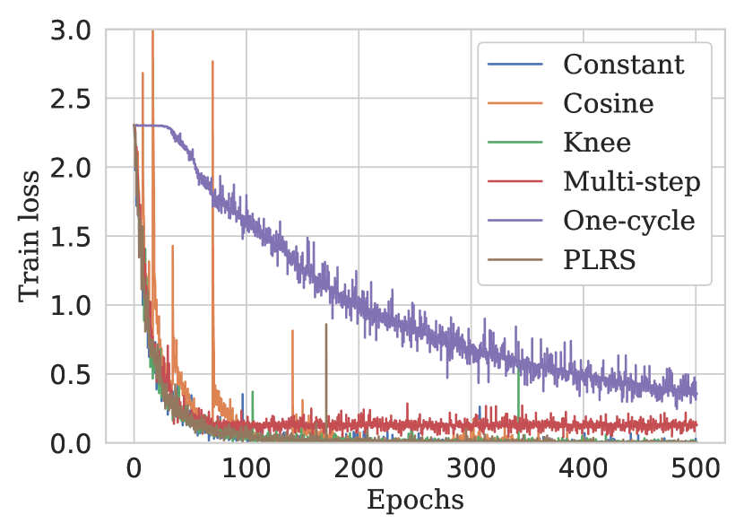
(a) VGG-16

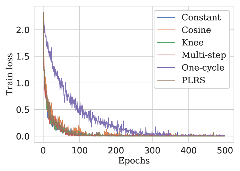
(b) WRN-28-10

Figure 1: Training loss vs epochs for VGG-16 and WRN-28-10 for CIFAR-10.

V-B Results for CIFAR-100

Architecture	Scheduler	Max acc.	Mean acc.(S.D)
ResNet-110	Cosine	74.22	72.66 (1.56)
ResNet-110	Knee	75.78	72.39 (2.96)
ResNet-110	One-cycle	71.09	70.05 (1.19)
ResNet-110	Constant	69.53	66.67 (2.51)
ResNet-110	Multi-step	63.28	61.20 (2.39)
ResNet-110	PLRS (ours)	77.34	74.61 (2.95)
DenseNet-40-12	Cosine	82.81	80.47 (2.07)
DenseNet-40-12	Knee	82.81	80.73 (2.39)
DenseNet-40-12	One-cycle	73.44	72.39 (0.90)
DenseNet-40-12	Constant	82.81	80.73 (2.39)
DenseNet-40-12	Multi-step	87.50	84.89 (2.39)
DenseNet-40-12	PLRS (ours)	84.37	83.33 (0.90)

Table II: Maximum and mean (with standard deviation) test accuracies over 3 runs with the CIFAR-100 dataset

We present results for experiments on the CIFAR-100 dataset using the ResNet-110 [8] and DenseNet-40-12 [29] networks in this section. We use $L_{min}=0.07$ and $L_{max}=0.1$ for ResNet-110, and $L_{min}=0.1$ and $L_{max}=0.2$ for DenseNet.

The maximum and the mean test accuracies (with standard deviation) across $3$ runs are provided in Table II. For ResNet-110, our proposed PLRS performs best in terms of the maximum and the mean test accuracies when compared to the other learning rate schedulers across $3$ runs. This is closely followed by the other state-of-the-art learning rate schedulers such as knee and cosine schedulers. For the DenseNet-40-12 network, PLRS comes to a close second to the multi-step learning rate scheduler in terms of the maximum and mean test accuracies. However, it is important to note that the multi-step scheduler records the least test accuracy with the ResNet-110 network. Hence, its performance is not consistent across the networks, while PLRS is consistently one of the best performing schedulers.

We also plot the training loss obtained across the epochs in Figure 2. With the ResNet-110 network, both PLRS and the knee learning rate scheduler converge to a low value of training loss around $150$ epochs. While the cosine annealing learning rate scheduler also seems to converge fast, it experiences sharp spikes along the curve during the restarts. With the DenseNet-40-12 network, our proposed PLRS clearly converges faster to lower training loss compared to the other learning rate schedulers.

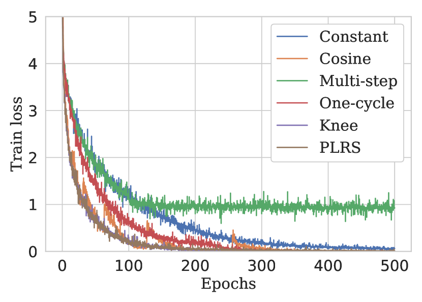
(a) ResNet-110

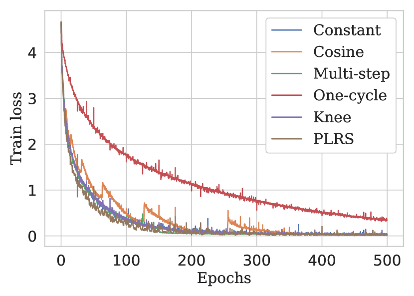
(b) DenseNet-40-12

Figure 2: Training loss vs epochs for ResNet-110 and DenseNet-40-12 on CIFAR-100.

V-C Results for Tiny ImageNet

We consider the Resnet-50 [8] architecture for our experiments with the Tiny ImageNet dataset. We use $L_{min}=0.35$ and $L_{max}=0.4$. We present the maximum and mean test accuracies across 3 runs in Table 4. We also provide the plot of training loss across the epochs in Figure 4. Our proposed PLRS performs the best in terms of maximum test accuracy. In terms of mean test accuracy, it ranks second next to cosine annealing by a close margin. Also, PLRS displays the best behaviour in terms of the convergence of training loss. It can be observed that it achieves the fastest convergence to the lowest training loss compared to the other baselines. Moreover, it exhibits steady convergence, especially when compared to its major competitor, cosine annealing, which experiences multiple spikes due to warm restarts.

Scheduler	Max acc.	Mean acc. (S.D)
Cosine	62.13	62.03 (0.15)
Knee	61.93	61.50 (0.42)
One-cycle	52.24	51.99 (0.22)
Constant	61.59	61.11 (0.42)
Multi-step	61.28	61.20 (0.08)
PLRS (ours)	62.34	61.90 (0.73)

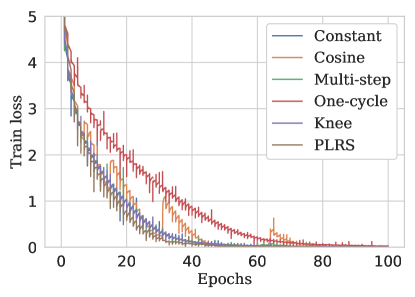
Figure 3: Maximum and mean (with standard deviation) test accuracies over 3 runs with Tiny ImageNet using ResNet-50.

Figure 4: Training loss vs epochs for ResNet-50 with Tiny ImageNet.

VI Concluding remarks

While there is a plethora of learning rate schedulers, we have proposed the novel idea of a probabilistic learning rate scheduler. The probabilistic nature of the scheduler helped us provide the first theoretical convergence proofs for SGD using learning rate schedulers. As we know, the theory in machine learning is always behind implementation and in our opinion, this is a significant step in the right direction to bridge the gap. We hope that this work inspires further theoretical exploration in justifying the use of learning rate schedulers. Our empirical results show that our proposed learning rate scheduler performs competitively with the state-of-the-art cyclic schedulers, if not better, on CIFAR-10, CIFAR-100, and Tiny ImageNet datasets for a wide variety of popular deep architectures. This leads us to hypothesize that the proposed probabilistic learning rate scheduler acts as a super-class of learning rate schedulers encompassing both probabilistic and deterministic schedulers. Future research directions include further exploration of this hypothesis.

Appendix A Proof of Theorem 1

Theorem 4 (Theorem 1 restated).

Under the assumptions A1 and A3 with $L_{max}<\frac{1}{\beta}$, for any point $\mathbf{x}_{t}$ with $\left\lVert\nabla f(\mathbf{x}_{t})\right\rVert\geq\sqrt{3\eta_{c}\beta\sigma^{2}}$ where $\sqrt{3\eta_{c}\beta\sigma^{2}}<\epsilon$ (satisfying B1), after one iteration we have,

$$\mathbb{E}[f(\mathbf{x}_{t+1})]-f(\mathbf{x}_{t})\leq-\tilde{\Omega}(L_{max}^{2}).$$

Proof.

Using the second order Taylor series approximation for $f(\textbf{x}_{t+1})$ around $\textbf{x}_{t}$, where $\mathbf{x}_{t+1}=\mathbf{x}_{t}-\eta_{c}\nabla f(\mathbf{x}_{t})-\mathbf{w}_{t}$, we have

$$f(\mathbf{x}_{t+1})-f(\mathbf{x}_{t}) \leq\nabla f(\mathbf{x}_{t})^{T}\left(\mathbf{x}_{t+1}-\mathbf{x}_{t}\right)+\frac{\beta}{2}\left\lVert\mathbf{x}_{t+1}-\mathbf{x}_{t}\right\rVert^{2},$$

following the result from [22, Lemma 1.2.3]. Taking expectation w.r.t. $\mathbf{w}_{t}$,

$$\mathbb{E}[f(\mathbf{x}_{t+1})]-f(\mathbf{x}_{t}) \leq\nabla f(\mathbf{x}_{t})^{T}\mathbb{E}[\mathbf{x}_{t+1}-\mathbf{x}_{t}]+\frac{\beta}{2}\mathbb{E}[\left\lVert\mathbf{x}_{t+1}-\mathbf{x}_{t}\right\rVert^{2}]$$ (4)

$$=\nabla f(\mathbf{x}_{t})^{T}\mathbb{E}[-\eta_{c}\nabla f(\mathbf{x}_{t})-\mathbf{w}_{t}]+\frac{\beta}{2}\mathbb{E}[\left\lVert-\eta_{c}\nabla f(\mathbf{x}_{t})-\mathbf{w}_{t}\right\rVert^{2}]$$

$$=-\eta_{c}\left\lVert\nabla f(\mathbf{x}_{t})\right\rVert^{2}+\frac{\beta}{2}\mathbb{E}[\eta_{c}^{2}\left\lVert\nabla f(\mathbf{x}_{t})\right\rVert^{2}+\left\lVert\mathbf{w}_{t}\right\rVert^{2}],$$

since $\mathbb{E}[\mathbf{w}_{t}]=0$ due to the zero mean property in Lemma 1. We focus on the last term in the next steps. Expanding $\left\lVert\mathbf{w}_{t}\right\rVert^{2}$,

$$\left\lVert\mathbf{w}_{t}\right\rVert^{2} =(\eta_{c}g(\mathbf{x}_{t})-\eta_{c}\nabla f(\mathbf{x}_{t})+u_{t+1}g(\mathbf{x}_{t}))^{T}(\eta_{c}g(\mathbf{x}_{t})-\eta_{c}\nabla f(\mathbf{x}_{t})+u_{t+1}g(\mathbf{x}_{t}))$$

$$=\eta_{c}^{2}\left\lVert g(\mathbf{x}_{t})\right\rVert^{2}-\eta_{c}^{2}g(\mathbf{x}_{t})^{T}\nabla f(\mathbf{x}_{t})+\eta_{c}u_{t+1}\left\lVert g(\mathbf{x}_{t})\right\rVert^{2}-\eta_{c}^{2}\nabla f(\mathbf{x}_{t})^{T}g(\mathbf{x}_{t})+\eta_{c}^{2}\left\lVert\nabla f(\mathbf{x}_{t}\right\rVert^{2}$$

$$-\eta_{c}u_{t+1}\nabla f(\mathbf{x}_{t})^{T}g(\mathbf{x}_{t})+\eta_{c}u_{t+1}\left\lVert g(\mathbf{x}_{t})\right\rVert^{2}-\eta_{c}u_{t+1}g(\mathbf{x}_{t})^{T}\nabla f(\mathbf{x}_{t})+u_{t+1}^{2}\left\lVert g(\mathbf{x}_{t})\right\rVert^{2}.$$

Taking expectation with respect to $\mathbf{x}_{t}$ and noting that $\mathbb{E}[u_{t+1}]=0$ and $\mathbb{E}[g(\mathbf{x}_{t})]=\nabla f(\mathbf{x}_{t})$,

$$\mathbb{E}[\left\lVert\mathbf{w}_{t}\right\rVert^{2}]=\eta_{c}^{2}\mathbb{E}[\left\lVert g(\mathbf{x}_{t})\right\rVert^{2}]-\eta_{c}^{2}\left\lVert\nabla f(\mathbf{x}_{t})\right\rVert^{2}+\mathbb{E}[u_{t+1}^{2}]\mathbb{E}[\left\lVert g(\mathbf{x}_{t})\right\rVert^{2}].$$ (5)

Now, as per assumption A3,

$$\left\lVert g(\mathbf{x}_{t})-\nabla f(\mathbf{x}_{t})\right\rVert^{2}\leq Q^{2}$$

$$\left\lVert g(\mathbf{x}_{t})\right\rVert^{2}+\left\lVert\nabla f(\mathbf{x}_{t})\right\rVert^{2}-2g(\mathbf{x}_{t})^{T}\nabla f(\mathbf{x}_{t})\leq Q^{2}$$

$$\left\lVert g(\mathbf{x}_{t})\right\rVert^{2}\leq Q^{2}-\left\lVert\nabla f(\mathbf{x}_{t})\right\rVert^{2}+2g(\mathbf{x}_{t})^{T}\nabla f(\mathbf{x}_{t})$$

$$\mathbb{E}[\left\lVert g(\mathbf{x}_{t})\right\rVert^{2}]\leq\mathbb{E}[Q^{2}]-\left\lVert\nabla f(\mathbf{x}_{t})\right\rVert^{2}+2\left\lVert\nabla f(\mathbf{x}_{t})\right\rVert^{2}\leq\sigma^{2}+\left\lVert\nabla f(\mathbf{x}_{t})\right\rVert^{2},$$ (6)

as $\mathbb{E}[Q^{2}]\leq\sigma^{2}$. Applying (6) to (5),

$$\mathbb{E}[\left\lVert\mathbf{w}_{t}\right\rVert^{2}] \leq\eta_{c}^{2}\sigma^{2}+\eta_{c}^{2}\left\lVert\nabla f(\mathbf{x}_{t})\right\rVert^{2}-\eta_{c}^{2}\left\lVert\nabla f(\mathbf{x}_{t})\right\rVert^{2}+\mathbb{E}[u_{t+1}^{2}]\sigma^{2}+\mathbb{E}[u_{t+1}^{2}]\left\lVert\nabla f(\mathbf{x}_{t})\right\rVert^{2}$$ (7)

$$=\eta_{c}^{2}\sigma^{2}+\mathbb{E}[u_{t+1}^{2}]\sigma^{2}+\mathbb{E}[u_{t+1}^{2}]\left\lVert\nabla f(\mathbf{x}_{t})\right\rVert^{2}$$

$$=\eta_{c}^{2}\sigma^{2}+\frac{(L_{max}-L_{min})^{2}\sigma^{2}}{12}+\frac{(L_{max}-L_{min})^{2}\left\lVert\nabla f(\textbf{x}_{0})\right\rVert^{2}}{12},$$

since the second moment of a uniformly distributed random variable in the interval $[L_{min}-\eta_{c},L_{max}-\eta_{c}]$ is given by $\frac{(L_{max}-L_{min})^{2}}{12}$. Using (7) in (4) and $\eta_{c}=\frac{L_{min}+L_{max}}{2}$,

$$\mathbb{E}[f(\mathbf{x}_{t+1})]-f(\mathbf{x}_{t}) \leq-\eta_{c}\left\lVert\nabla f(\mathbf{x}_{t})\right\rVert^{2}+\frac{\beta}{2}\eta_{c}^{2}\left\lVert\nabla f(\mathbf{x}_{t})\right\rVert^{2}+\frac{\beta\eta_{c}^{2}\sigma^{2}}{2}+\frac{\beta(L_{max}-L_{min})^{2}\sigma^{2}}{24}$$

$$+\frac{\beta(L_{max}-L_{min})^{2}\left\lVert\nabla f(\mathbf{x}_{t})\right\rVert^{2}}{24}$$

$$\leq-\eta_{c}\left\lVert\nabla f(\mathbf{x}_{t})\right\rVert^{2}+\frac{\beta}{2}\eta_{c}^{2}\left\lVert\nabla f(\mathbf{x}_{t})\right\rVert^{2}+\frac{\beta\eta_{c}^{2}\sigma^{2}}{2}+\frac{\beta\eta_{c}^{2}\sigma^{2}}{6}+\frac{\beta\eta_{c}^{2}\left\lVert\nabla f(\textbf{x}_{0})\right\rVert^{2}}{6}$$

$$=-\left\lVert\nabla f(\mathbf{x}_{t})\right\rVert^{2}\left(\eta_{c}-\frac{2\beta\eta_{c}^{2}}{3}\right)+\frac{2\beta\eta_{c}^{2}\sigma^{2}}{3}$$

Now, applying our initial assumption that $\left\lVert\nabla f(\mathbf{x}_{t})\right\rVert\geq\sqrt{3\eta_{c}\beta\sigma^{2}}$, we have,

$$\mathbb{E}[f(\mathbf{x}_{t+1})]-f(\mathbf{x}_{t})\leq-3\eta_{c}\beta\sigma^{2}\left(\eta_{c}-\frac{2\beta\eta_{c}^{2}}{3}\right)+\frac{2\beta\eta_{c}^{2}\sigma^{2}}{3}=-3\eta_{c}^{2}\beta\sigma^{2}+\frac{6\beta^{2}\eta_{c}^{3}\sigma^{2}}{3}+\frac{2\beta\eta_{c}^{2}\sigma^{2}}{3}$$

Since $L_{max}<\frac{1}{\beta}$ and $\eta_{c}=\frac{L_{min}+L_{max}}{2}$, we have $\eta_{c}\beta<L_{max}\beta<1$. Finally,

$$\mathbb{E}[f(\mathbf{x}_{t+1})]-f(\mathbf{x}_{t}) \leq-3\eta_{c}^{2}\beta\sigma^{2}+\frac{6\beta\eta_{c}^{2}\sigma^{2}}{3}+\frac{2\beta\eta_{c}^{2}\sigma^{2}}{3}=-\frac{\beta\eta_{c}^{2}\sigma^{2}}{3}$$

$$=-\tilde{\Omega}(\eta_{c}^{2}),$$

which proves the theorem. ∎

Appendix B Additional results needed to prove Theorem 2

Here, we state and prove two lemmas that are instrumental in the proof of Theorem 2.

B-A Proof of Lemma 2

In the following Lemma, we prove that the gradients of a second order approximation of $f$ are probabilistically bounded for all $t\leq T$ and its iterates as we apply SGD-PLRS are also bounded when the initial iterate $\textbf{x}_{0}$ is a saddle point.

Lemma 2.

Let $f$ satisfy Assumptions A1 - A4. Let $\tilde{f}$ be the second order Taylor approximation of $f$ and let $\tilde{\textbf{x}}_{t}$ be the iterate at time step $t$ obtained using the SGD update equation as in (1) on $\tilde{f}$; let $\tilde{\textbf{x}}_{0}=\textbf{x}_{0}$, $\left\lVert\nabla f(\textbf{x}_{0})\right\rVert\leq\epsilon$ and the minimum eigenvalue of the Hessian of $f$ at $\textbf{x}_{0}$ be $\lambda_{min}(\textbf{H}(\textbf{x}_{0}))=-\gamma_{o}$ where $\gamma_{o}>0$. With probability at least $1-\tilde{O}(L_{max}^{15/4})$, we have

$$\left\lVert\nabla\tilde{f}(\tilde{\textbf{x}}_{t})\right\rVert\leq\tilde{O}\left(\frac{1}{L_{max}^{0.5}}\right),\quad\left\lVert\tilde{\textbf{x}}_{t}-\textbf{x}_{0}\right\rVert\leq\tilde{O}\left(L_{max}^{3/8}\log\left(\frac{1}{L_{max}}\right)\right)\quad\forall t\leq T=\tilde{O}\left(L_{max}^{-1/4}\right).$$

Proof.

As $\tilde{f}$ is the second order Taylor series approximation of $f$, we have

$$\tilde{f}(\tilde{\textbf{x}})=f(\textbf{x}_{0})+\nabla f(\textbf{x}_{0})^{T}(\tilde{\textbf{x}}-\textbf{x}_{0})+\frac{1}{2}(\tilde{\textbf{x}}-\textbf{x}_{0})^{T}\textbf{H}(\textbf{x}_{0})(\tilde{\textbf{x}}-\textbf{x}_{0}).$$

Taking derivative w.r.t. $\tilde{\textbf{x}}$, we have $\nabla\tilde{f}(\tilde{\textbf{x}})=\nabla f(\textbf{x}_{0})+\textbf{H}(\textbf{x}_{0})(\tilde{\textbf{x}}-\textbf{x}_{0}).$ Now, note that $\nabla\tilde{f}(\tilde{\textbf{x}}_{t-1})=\nabla f(\textbf{x}_{0})+\textbf{H}(\textbf{x}_{0})(\tilde{\textbf{x}}_{t-1}-\textbf{x}_{0})=K(\textbf{x}_{0})+\textbf{H}(\textbf{x}_{0})\tilde{\textbf{x}}_{t-1}$, where $K(\textbf{x}_{0})=\nabla f(\textbf{x}_{0})-\textbf{H}(\textbf{x}_{0})\textbf{x}_{0}=\nabla\tilde{f}(\tilde{\textbf{x}}_{t-1})-\textbf{H}(\textbf{x}_{0})\tilde{\textbf{x}}_{t-1}$. Therefore,

$$\nabla\tilde{f}(\tilde{\textbf{x}}_{t})=K(\textbf{x}_{0})+\textbf{H}(\textbf{x}_{0})\tilde{\textbf{x}}_{t} =\nabla\tilde{f}(\tilde{\textbf{x}}_{t-1})-\textbf{H}(\textbf{x}_{0})\tilde{\textbf{x}}_{t-1}+\textbf{H}(\textbf{x}_{0})\tilde{\textbf{x}}_{t}$$ (8)

$$=\nabla\tilde{f}(\tilde{\textbf{x}}_{t-1})+\textbf{H}(\textbf{x}_{0})(\tilde{\textbf{x}}_{t}-\tilde{\textbf{x}}_{t-1}).$$

Next, using the SGD-PLRS update and rearranging,

$$\nabla\tilde{f}(\tilde{\textbf{x}}_{t}) =\nabla\tilde{f}(\tilde{\textbf{x}}_{t-1})-\textbf{H}(\textbf{x}_{0})(\eta_{c}\nabla\tilde{f}(\tilde{\textbf{x}}_{t-1})+\tilde{\textbf{w}}_{t-1})$$ (9)

$$=(I-\eta_{c}\textbf{H}(\textbf{x}_{0}))\nabla\tilde{f}(\tilde{\textbf{x}}_{t-1})-\textbf{H}(\textbf{x}_{0})\tilde{\textbf{w}}_{t-1},$$

where $I$ denotes the $d\times d$ identity matrix. Next, unrolling the term $\nabla\tilde{f}(\tilde{\textbf{x}}_{t-1})$ recursively,

$$\nabla\tilde{f}(\tilde{\textbf{x}}_{t})=(I-\eta_{c}\textbf{H}(\textbf{x}_{0}))^{t}\nabla\tilde{f}(\tilde{\textbf{x}}_{0})-\textbf{H}(\textbf{x}_{0})\sum_{\tau=0}^{t-1}(I-\eta_{c}\textbf{H}(\textbf{x}_{0}))^{t-\tau-1}\tilde{\textbf{w}}_{\tau}.$$ (10)

Using the triangle and Cauchy-Schwartz inequalities,

$$\left\lVert\nabla\tilde{f}(\tilde{\textbf{x}}_{t})\right\rVert \leq\left\lVert(I-\eta_{c}\textbf{H}(\textbf{x}_{0}))^{t}\nabla\tilde{f}(\tilde{\textbf{x}}_{0})\right\rVert+\left\lVert\textbf{H}(\textbf{x}_{0})\sum_{\tau=0}^{t-1}(I-\eta_{c}\textbf{H}(\textbf{x}_{0}))^{t-\tau-1}\tilde{\textbf{w}}_{\tau}\right\rVert$$ (11)

$$\leq\left\lVert(I-\eta_{c}\textbf{H}(\textbf{x}_{0}))^{t}\right\rVert\;\left\lVert\nabla\tilde{f}(\tilde{\textbf{x}}_{0})\right\rVert+\left\lVert\textbf{H}(\textbf{x}_{0})\right\rVert\;\left\lVert\sum_{\tau=0}^{t-1}(I-\eta_{c}\textbf{H}(\textbf{x}_{0}))^{t-\tau-1}\tilde{\textbf{w}}_{\tau}\right\rVert$$

Note that the norm over the matrices refers to the matrix-induced norm. Since $\textbf{H}(\textbf{x}_{0})$ is a real symmetric matrix, the induced norm gives the maximum eigenvalue of $\textbf{H}(\textbf{x}_{0})$ i.e, $\lambda_{max}(\textbf{H}(\textbf{x}_{0}))\leq\beta$ by our $\beta$-smoothness assumption A1. In the case of $(I-\eta_{c}\textbf{H}(\textbf{x}_{0}))$ the induced norm gives $(1-\eta_{c}\lambda_{min}(\textbf{H}(\textbf{x}_{0}))$ which is $(1+\eta_{c}\gamma_{o})$ as per our assumption that $\lambda_{min}(\textbf{H}(\textbf{x}_{0}))=-\gamma_{o}$. Also recall that $\left\lVert\nabla\tilde{f}(\tilde{\textbf{x}}_{0})\right\rVert\leq\epsilon$. Now (11) becomes,

$$\left\lVert\nabla\tilde{f}(\tilde{\textbf{x}}_{t})\right\rVert \leq(1+\eta_{c}\gamma_{o})^{t}\epsilon+\beta\;\left\lVert\sum_{\tau=0}^{t-1}(I-\eta_{c}\textbf{H}(\textbf{x}_{0}))^{t-\tau-1}\tilde{\textbf{w}}_{\tau}\right\rVert,$$ (12)

$$\leq(1+\eta_{c}\gamma_{o})^{t}\epsilon+\beta\sum_{\tau=0}^{t-1}(1+\eta_{c}\gamma_{o})^{t-\tau-1}\left\lVert\tilde{\textbf{w}}_{\tau}\right\rVert.$$

Now, expanding the noise term $\tilde{\textbf{w}}_{\tau}$,

$$\left\lVert\nabla\tilde{f}(\tilde{\textbf{x}}_{t})\right\rVert=(1+\eta_{c}\gamma_{o})^{t}\epsilon+\beta\sum_{\tau=0}^{t-1}(1+\eta_{c}\gamma_{o})^{t-\tau-1}\left\lVert\eta_{c}\tilde{g}(\tilde{\textbf{x}}_{\tau})-\eta_{c}\nabla\tilde{f}(\tilde{\textbf{x}}_{\tau})+u_{\tau+1}\tilde{g}(\tilde{\textbf{x}}_{\tau})\right\rVert$$

Now recall from our assumption A3 that $\left\lVert\tilde{g}(\tilde{\textbf{x}}_{\tau})-\nabla\tilde{f}(\tilde{\textbf{x}}_{\tau})\right\rVert\leq\tilde{Q}$. Hence,

$$\left\lVert\nabla\tilde{f}(\tilde{\textbf{x}}_{t})\right\rVert \leq(1+\eta_{c}\gamma_{o})^{t}\epsilon+\beta\sum_{\tau=0}^{t-1}(1+\eta_{c}\gamma_{o})^{t-\tau-1}\left(\eta_{c}\tilde{Q}+|u_{\tau+1}|\left\lVert\tilde{g}(\tilde{\textbf{x}}_{\tau})-\nabla\tilde{f}(\tilde{\textbf{x}}_{\tau})+\nabla\tilde{f}(\tilde{\textbf{x}}_{\tau})\right\rVert\right)$$

$$\leq(1+\eta_{c}\gamma_{o})^{t}\epsilon+\beta\sum_{\tau=0}^{t-1}(1+\eta_{c}\gamma_{o})^{t-\tau-1}\left(\eta_{c}\tilde{Q}+|u_{\tau+1}|\left(\tilde{Q}+\left\lVert\nabla\tilde{f}(\tilde{\textbf{x}}_{\tau})\right\rVert\right)\right)$$

Using $\left\lVert\nabla\tilde{f}(\tilde{\textbf{x}}_{0})\right\rVert\leq\epsilon$ and $\left\lVert\nabla\tilde{f}(\tilde{\textbf{x}}_{1})\right\rVert\leq(1+\eta_{c}\gamma_{o})\epsilon+\epsilon+2\tilde{Q}$, it can be proved by induction that the general expression for $t\geq 2$ is given by,

$$\left\lVert\nabla\tilde{f}(\tilde{\textbf{x}}_{t})\right\rVert\leq 10\tilde{Q}\sum_{\tau=0}^{\frac{t(t-1)}{2}}(1+\eta_{c}\gamma_{o})^{\tau}$$ (13)

We give the proof of (13) by induction in Appendix E. Next, we prove the bound on $\tilde{\textbf{x}}_{t}-\tilde{\textbf{x}}_{0}$. Using the SGD-PLRS update,

$$\tilde{\textbf{x}}_{t}-\tilde{\textbf{x}}_{0}=-\sum_{\tau=0}^{t-1}\left(\eta_{c}\nabla\tilde{f}(\tilde{\textbf{x}}_{\tau})+\tilde{\textbf{w}}_{\tau}\right)$$

$$=-\sum_{\tau=0}^{t-1}\left(\eta_{c}\left((I-\eta_{c}\textbf{H}(\textbf{x}_{0}))^{\tau}\nabla\tilde{f}(\tilde{\textbf{x}}_{0})-\textbf{H}(\textbf{x}_{0})\sum_{\tau^{{}^{\prime}}=0}^{\tau-1}(I-\eta_{c}\textbf{H}(\textbf{x}_{0}))^{\tau-\tau^{{}^{\prime}}-1}\tilde{\textbf{w}}_{\tau^{{}^{\prime}}}\right)+\tilde{\textbf{w}}_{\tau}\right)$$ (14a)

$$=-\sum_{\tau=0}^{t-1}\eta_{c}(I-\eta_{c}\textbf{H}(\textbf{x}_{0}))^{\tau}\nabla f(\textbf{x}_{0})-\sum_{\tau=0}^{t-1}(I-\eta_{c}\textbf{H}(\textbf{x}_{0}))^{t-\tau-1}\tilde{\textbf{w}}_{\tau},$$ (14b)

where the equation (14a) is obtained by using (10). We obtain (14b) by using the summation of geometric series as $\textbf{H}(\textbf{x}_{0})$ is invertible by the strict saddle property. As $\tilde{\textbf{x}}_{0}=\textbf{x}_{0}$, we can write $\nabla\tilde{f}(\tilde{\textbf{x}}_{0})=\nabla f(\textbf{x}_{0})$. Taking norm,

$$\left\lVert\tilde{\textbf{x}_{t}}-\tilde{\textbf{x}}_{0}\right\rVert \leq\left\lVert\sum_{\tau=0}^{t-1}\eta_{c}(I-\eta_{c}\textbf{H}(\textbf{x}_{0}))^{\tau}\nabla f(\textbf{x}_{0})\right\rVert+\left\lVert\sum_{\tau=0}^{t-1}(I-\eta_{c}\textbf{H}(\textbf{x}_{0}))^{t-\tau-1}\tilde{\textbf{w}}_{\tau}\right\rVert$$ (15)

$$\leq\sum_{\tau=0}^{t-1}\left\lVert\eta_{c}(I-\eta_{c}\textbf{H}(\textbf{x}_{0}))^{\tau}\nabla f(\textbf{x}_{0})\right\rVert+\sum_{\tau=0}^{t-1}\left\lVert(I-\eta_{c}\textbf{H}(\textbf{x}_{0}))^{t-\tau-1}\tilde{\textbf{w}}_{\tau}\right\rVert$$

$$\leq\eta_{c}\epsilon\sum_{\tau=0}^{t-1}(1+\eta_{c}\gamma_{o})^{\tau}+\sum_{\tau=0}^{t-1}(1+\eta_{c}\gamma_{o})^{t-\tau-1}\left\lVert\tilde{\textbf{w}}_{\tau}\right\rVert.$$

In (15), it can be seen that the first term is arbitrarily small by the initial assumption and that the second term decides the order of $\left\lVert\tilde{\textbf{x}}_{t}-\tilde{\textbf{x}}_{0}\right\rVert$. Hence, in order to bound $\left\lVert\tilde{\textbf{x}_{t}}-\tilde{\textbf{x}}_{0}\right\rVert$ probabilistically, it is sufficient to bound the second term, $\sum_{\tau=0}^{t-1}(1+\eta_{c}\gamma_{o})^{t-\tau-1}\left\lVert\tilde{\textbf{w}}_{\tau}\right\rVert$. Now,

$$\sum_{\tau=0}^{t-1}(1+\eta_{c}\gamma_{o})^{t-\tau-1}\left\lVert\tilde{\textbf{w}}_{\tau}\right\rVert =\sum_{\tau=0}^{t-1}(1+\eta_{c}\gamma_{o})^{t-\tau-1}\left\lVert\eta_{c}\tilde{g}(\tilde{\textbf{x}}_{\tau})-\eta_{c}\nabla\tilde{f}(\tilde{\textbf{x}}_{\tau})+u_{\tau+1}\tilde{g}(\tilde{\textbf{x}}_{\tau})\right\rVert$$

$$=\sum_{\tau=0}^{t-1}(1+\eta_{c}\gamma_{o})^{t-\tau-1}\left(\eta_{c}\tilde{Q}+\left\lvert u_{\tau+1}\right\rvert\left\lVert\tilde{g}(\tilde{\textbf{x}}_{\tau})-\nabla\tilde{f}(\tilde{\textbf{x}}_{\tau})+\nabla\tilde{f}(\tilde{\textbf{x}}_{\tau})\right\rVert\right)$$

$$=\sum_{\tau=0}^{t-1}(1+\eta_{c}\gamma_{o})^{t-\tau-1}\tilde{Q}\left(\eta_{c}+\left\lvert u_{\tau+1}\right\rvert\right)+\sum_{\tau=0}^{t-1}(1+\eta_{c}\gamma_{o})^{t-\tau-1}\left\lvert u_{\tau+1}\right\rvert\left\lVert\nabla\tilde{f}(\tilde{\textbf{x}}_{\tau})\right\rVert$$

Now, using $\left\lVert\nabla\tilde{f}(\tilde{\textbf{x}}_{0})\right\rVert\leq\epsilon$, $\left\lVert\nabla\tilde{f}(\tilde{\textbf{x}}_{1})\right\rVert\leq(1+\eta_{c}\gamma_{o})\epsilon+\epsilon+2\tilde{Q}$ and (13) we write,

$$\sum_{\tau=0}^{t-1}(1+\eta_{c}\gamma_{o})^{t-\tau-1}\left\lVert\tilde{\textbf{w}}_{\tau}\right\rVert\leq\sum_{\tau=0}^{t-1}(1+\eta_{c}\gamma_{o})^{t-\tau-1}\tilde{Q}\left(\eta_{c}+\left\lvert u_{\tau+1}\right\rvert\right)+(1+\eta_{c}\gamma_{o})^{t-1}\left\lvert u_{1}\right\rvert\epsilon+$$ (16)

$$(1+\eta_{c}\gamma_{o})^{t-2}\left\lvert u_{2}\right\rvert\left((1+\eta_{c}\gamma_{o})\epsilon+\epsilon+2\tilde{Q}\right)+\sum_{\tau=2}^{t-1}(1+\eta_{c}\gamma_{o})^{t-\tau-1}\left\lvert u_{\tau+1}\right\rvert 10\tilde{Q}\sum_{\tau^{{}^{\prime}}=0}^{\frac{\tau(\tau-1)}{2}}(1+\eta_{c}\gamma_{o})^{\tau^{{}^{\prime}}}$$

It can be observed from (16) that the last term dominates the expression of and hence, it determines the order of $\left\lVert\tilde{\textbf{x}}_{t}-\tilde{\textbf{x}}_{0}\right\rVert$. We now apply Hoeffding’s inequality to derive a probabilistic bound on $\left\lVert\tilde{\textbf{x}_{t}}-\tilde{\textbf{x}}_{0}\right\rVert$. According to Hoeffding’s inequality for any summation $S_{n}=X_{1}+\cdots+X_{n}$ such that $a_{i}\leq X_{i}\leq b_{i}$, $\mathbb{P}\left(S_{n}-\mathbb{E}[S_{n}]\geq\delta\right)\leq\exp\left(\frac{-2\delta^{2}}{\sum_{i=1}^{n}(b_{i}-a_{i})^{2}}\right)$. Now, setting $T=\tilde{O}\left(L_{max}^{-1/4}\right)$ from (35) and assuming $\eta_{c}\leq\eta_{max}\leq\frac{\sqrt{2}-1}{\gamma^{{}^{\prime}}},\gamma_{o}\leq\gamma^{{}^{\prime}}$, the squared bound of the summation $\sum_{\tau=2}^{t-1}(1+\eta_{c}\gamma_{o})^{t-\tau-1}\left\lvert u_{\tau+1}\right\rvert 10\tilde{Q}\sum_{\tau^{{}^{\prime}}=0}^{\frac{\tau(\tau-1)}{2}}(1+\eta_{c}\gamma_{o})^{\tau^{{}^{\prime}}}\leq\tilde{O}\left(L_{max}^{3/4}\right)$, Setting $\delta=\tilde{O}\left(\sqrt{L_{max}^{3/4}}\log\left(\frac{1}{L_{max}}\right)\right)$, for some $t\leq T$,

$$\mathbb{P}\left(\sum_{\tau=2}^{t-1}(1+\eta_{c}\gamma_{o})^{t-\tau-1}\left\lvert u_{\tau+1}\right\rvert 10\tilde{Q}\sum_{\tau^{{}^{\prime}}=0}^{\frac{\tau(\tau-1)}{2}}(1+\eta_{c}\gamma_{o})^{\tau^{{}^{\prime}}}\geq\tilde{O}\left(L_{max}^{3/8}\log\left(\frac{1}{L_{max}}\right)\right)\right)$$

$$\leq\tilde{O}(L^{4}_{max}).$$

Taking the union bound over all $t\leq T$,

$$\mathbb{P}\left(\forall t\leq T,\quad\sum_{\tau=2}^{t-1}(1+\eta_{c}\gamma_{o})^{t-\tau-1}\left\lvert u_{\tau+1}\right\rvert 10\tilde{Q}\sum_{\tau^{{}^{\prime}}=0}^{\frac{\tau(\tau-1)}{2}}(1+\eta_{c}\gamma_{o})^{\tau^{{}^{\prime}}}\geq\tilde{O}\left(L_{max}^{3/8}\log\left(\frac{1}{L_{max}}\right)\right)\right)$$

$$\leq\tilde{O}\left(L_{max}^{15/4}\right),$$

which completes our proof. ∎

B-B Proof of Lemma 3

This lemma is used to derive an expression for a high probability upper bound of $\left\lVert\textbf{x}_{t}-\tilde{\textbf{x}}_{t}\right\rVert$ and $\left\lVert\nabla f(\textbf{x}_{t})-\nabla\tilde{f}(\tilde{\textbf{x}}_{t})\right\rVert$.

Lemma 3.

Let $f:\mathbb{R}^{d}\rightarrow\mathbb{R}$ satisfy Assumptions A1 - A4. Let $\tilde{f}$ be the second order Taylor’s approximation of $f$ and let $\textbf{x}_{t}$, $\tilde{\textbf{x}}_{t}$ be the iterates at time step $t$ obtained using the SGD-PLRS update on $f$, $\tilde{f}$ respectively; let $\tilde{\textbf{x}}_{0}=\textbf{x}_{0}$ and $\left\lVert\nabla f(\textbf{x}_{0})\right\rVert\leq\epsilon$. Let the minimum eigenvalue of the Hessian at $\textbf{x}_{0}$ be $\lambda_{min}(\nabla^{2}(f(\textbf{x}_{0})))=-\gamma_{o}$, where $\gamma_{o}>0$. Then $\forall t\leq T=O\left(L_{max}^{-1/4}\right)$, with a probability of at least $1-\tilde{O}(L_{max}^{7/2})$,

$$\left\lVert\textbf{x}_{t}-\tilde{\textbf{x}}_{t}\right\rVert \leq O\left(L_{max}^{3/4}\right)\quad\text{ and }\quad\left\lVert\nabla f(\textbf{x}_{t})-\nabla\tilde{f}(\tilde{\textbf{x}}_{t})\right\rVert \leq O\left(L_{max}^{3/8}\log\frac{1}{L_{max}}\right).$$

Proof.

The expression for $\textbf{x}_{t}-\tilde{\textbf{x}}_{t}$ can be written as,

$$\textbf{x}_{t}-\tilde{\textbf{x}}_{t} =(\textbf{x}_{t}-\textbf{x}_{0})-(\tilde{\textbf{x}}_{t}-\textbf{x}_{0})$$ (17)

$$=-\sum_{\tau=0}^{t-1}\big{(}\eta_{c}\nabla f(\textbf{x}_{\tau})+\textbf{w}_{\tau}\big{)}-\left(-\sum_{\tau=0}^{t-1}\big{(}\eta_{c}\nabla\tilde{f}(\tilde{\textbf{x}}_{\tau})+\tilde{\textbf{w}}_{\tau}\big{)}\right)=-\sum_{\tau=0}^{t-1}\left(\eta_{c}\Delta_{\tau}+(\textbf{w}_{\tau}-\tilde{\textbf{w}}_{\tau})\right).$$

where we define $\Delta_{t}=\nabla f(\textbf{x}_{t})-\nabla\tilde{f}(\tilde{\textbf{x}}_{t})$. Now in order to bound $\left\lVert\textbf{x}_{t}-\tilde{\textbf{x}}_{t}\right\rVert$, we derive expressions for both $\textbf{w}_{\tau}-\tilde{\textbf{w}}_{\tau}$ and $\Delta_{\tau}$. We initially focus on the term $\textbf{w}_{\tau}-\tilde{\textbf{w}}_{\tau}$.

$$\textbf{w}_{\tau}-\tilde{\textbf{w}}_{\tau} =\eta_{c}g(\textbf{x}_{\tau})-\eta_{c}\nabla f_{\tau}+u_{\tau+1}g(\textbf{x}_{\tau})-\left(\eta_{c}\tilde{g}(\tilde{\textbf{x}}_{\tau})-\eta_{c}\nabla\tilde{f}(\tilde{\textbf{x}}_{\tau})+u_{\tau+1}\tilde{g}(\tilde{\textbf{x}}_{\tau})\right)$$ (18)

$$=\left(u_{\tau+1}+\eta_{c}\right)\left(\big{(}g(\textbf{x}_{\tau})-\nabla f(\textbf{x}_{\tau})\big{)}-\big{(}\tilde{g}(\tilde{\textbf{x}}_{\tau})-\nabla\tilde{f}(\tilde{\textbf{x}}_{\tau})\big{)}\right)+u_{\tau+1}\Delta_{\tau}.$$

Taking norm on both sides,

$$\left\lVert\textbf{w}_{\tau}-\tilde{\textbf{w}}_{\tau}\right\rVert\leq\left\lvert u_{\tau+1}+\eta_{c}\right\rvert\left(Q+\tilde{Q}\right)+\left\lvert u_{\tau+1}\right\rvert\left\lVert\Delta_{\tau}\right\rVert$$ (19)

Using (18) and (19) in (17), and assumption A3 that stochastic noise is bounded, and applying norm,

$$\left\lVert\textbf{x}_{t}-\tilde{\textbf{x}}_{t}\right\rVert =\left\lVert-\sum_{\tau=0}^{t-1}\left(\eta_{c}\Delta_{\tau}+(\textbf{w}_{\tau}-\tilde{\textbf{w}}_{\tau})\right)\right\rVert\leq\sum_{\tau=0}^{t-1}\left\lVert\eta_{c}\Delta_{\tau}+(\textbf{w}_{\tau}-\tilde{\textbf{w}}_{\tau})\right\rVert$$ (20)

$$\leq\sum_{\tau=0}^{t-1}(\eta_{c}+\left\lvert u_{\tau+1}\right\rvert)\left(\left\lVert\Delta_{\tau}\right\rVert+Q+\tilde{Q}\right)$$

Next, we focus on providing a bound for $\left\lVert\Delta_{t}\right\rVert$. Recall that $\Delta_{t}=\nabla f(\textbf{x}_{t})-\nabla\tilde{f}(\tilde{\textbf{x}}_{t})$. The gradient can be written as [22],

$$\nabla f(\textbf{x}_{t}) =\nabla f(\textbf{x}_{t-1})+(\textbf{x}_{t}-\textbf{x}_{t-1})\left(\int_{0}^{1}\textbf{H}(\textbf{x}_{t-1}+v(\textbf{x}_{t}-\textbf{x}_{t-1}))dv\right)$$

$$=\nabla f(\textbf{x}_{t-1})+(\textbf{x}_{t}-\textbf{x}_{t-1})\left(\int_{0}^{1}\big{(}\textbf{H}(\textbf{x}_{t-1}+v(\textbf{x}_{t}-\textbf{x}_{t-1}))+\textbf{H}(\textbf{x}_{t-1})-\textbf{H}(\textbf{x}_{t-1})\big{)}dv\right)$$

$$=\nabla f(\textbf{x}_{t-1})+\textbf{H}(\textbf{x}_{t-1})(\textbf{x}_{t}-\textbf{x}_{t-1})+\theta_{t-1},$$

where $\theta_{t-1}=\left(\int_{0}^{1}\big{(}\textbf{H}(\textbf{x}_{t-1}+v(\textbf{x}_{t}-\textbf{x}_{t-1}))-\textbf{H}(\textbf{x}_{t-1})\big{)}dv\right)(\textbf{x}_{t}-\textbf{x}_{t-1})$. Let $H^{{}^{\prime}}_{t-1}=\textbf{H}(\textbf{x}_{t-1})-\textbf{H}(\textbf{x}_{0})$. Using the SGD-PLRS update,

$$\nabla f(\textbf{x}_{t}) =\nabla f(\textbf{x}_{t-1})-(H_{t-1}^{{}^{\prime}}+\textbf{H}(\textbf{x}_{0}))(\eta_{c}\nabla f(\textbf{x}_{t-1})+\textbf{w}_{t-1})+\theta_{t-1}$$ (21)

$$=\nabla f(\textbf{x}_{t-1})(I-\eta_{c}\textbf{H}(\textbf{x}_{0}))-\textbf{H}(\textbf{x}_{0})\textbf{w}_{t-1}-\eta_{c}H^{{}^{\prime}}_{t-1}\nabla f(\textbf{x}_{t-1})-H^{{}^{\prime}}_{t-1}\textbf{w}_{t-1}+\theta_{t-1},$$

From (8) in the proof of Lemma 2,

$$\nabla\tilde{f}(\tilde{\textbf{x}}_{t})=\nabla\tilde{f}(\tilde{\textbf{x}}_{t-1})+\textbf{H}(\textbf{x}_{0})(\tilde{\textbf{x}}_{t}-\tilde{\textbf{x}}_{t-1}).$$ (22)

Subtracting (22) from (21), we obtain $\Delta_{t}$ as,

$$\Delta_{t} =\nabla f(\textbf{x}_{t-1})(I-\eta_{c}\textbf{H}(\textbf{x}_{0}))-\textbf{H}(\textbf{x}_{0})\textbf{w}_{t-1}-\eta_{c}H^{{}^{\prime}}_{t-1}\nabla f(\textbf{x}_{t-1})-H^{{}^{\prime}}_{t-1}\textbf{w}_{t-1}+\theta_{t-1}$$ (23)

$$\hskip 240.00037pt-\nabla\tilde{f}(\tilde{\textbf{x}}_{t-1})-\textbf{H}(\textbf{x}_{0})(\tilde{\textbf{x}}_{t}-\tilde{\textbf{x}}_{t-1})$$

$$=(I-\eta_{c}\textbf{H}(\textbf{x}_{0}))\Delta_{t-1}-\textbf{H}(\textbf{x}_{0})\left(\textbf{w}_{t-1}-\tilde{\textbf{w}}_{t-1}\right)-H^{{}^{\prime}}_{t-1}\big{(}\eta_{c}\Delta_{t-1}+\eta_{c}\nabla\tilde{f}(\tilde{\textbf{x}}_{t-1})\big{)}$$

$$\hskip 240.00037pt-H^{{}^{\prime}}_{t-1}\textbf{w}_{t-1}+\theta_{t-1},$$

We now have an expression for $\Delta_{t}$. However, the derived expression is recursive and contains $\Delta_{t-1}$. We focus on eliminating the recursive dependence and obtain a stand-alone bound for $\left\lVert\Delta_{t}\right\rVert$ $\forall t\leq T$. Now, we bound each of the five terms (we term them $T_{1},\cdots,T_{5}$) of (23). First, let us define the events,

$$R_{t} =\left\{\forall\tau\leq t,\quad\left\lVert\nabla\tilde{f}(\tilde{\textbf{x}}_{\tau})\right\rVert\leq\tilde{O}\left(\frac{1}{\sqrt{L_{max}}}\right),\quad\left\lVert\tilde{\textbf{x}}_{\tau}-\textbf{x}_{0}\right\rVert\leq\tilde{O}\left(L_{max}^{3/8}\log\left(\frac{1}{L_{max}}\right)\right)\right\}$$

$$C_{t} =\left\{\forall\tau\leq t,\quad\left\lVert\Delta_{\tau}\right\rVert\leq\mu L_{max}^{3/8}\log\left(\frac{1}{L_{max}}\right)\right\}.$$

It can be seen that $R_{t}\subset R_{t-1}$ and $C_{t}\subset C_{t-1}$. Note that, from Lemma 2, we know the probabilistic characterization of $R_{t}$. We comment on the parameter $\mu$ later in the proof. Now, we derive bounds for each term of $\Delta_{t}$ conditioned on the event $R_{t-1}\cap C_{t-1}$ for time $t\leq T=O\left(L_{max}^{-1/4}\right)$.

$$T_{1}:\quad\left\lVert(I-\eta_{c}\textbf{H}(\textbf{x}_{0}))\Delta_{t-1}\right\rVert \leq\left\lVert\Delta_{t-1}\right\rVert+\left\lVert-\eta_{c}\textbf{H}(\textbf{x}_{0})\Delta_{t-1}\right\rVert$$ (24)

$$\leq\mu L_{max}^{3/8}\log\left(\frac{1}{L_{max}}\right)+\tilde{O}\left(\mu L_{max}^{11/8}\log\left(\frac{1}{L_{max}}\right)\right)$$

$$=\tilde{O}\left(\mu L_{max}^{3/8}\log\left(\frac{1}{L_{max}}\right)\right),$$

where (24) follows from the definition of event $C_{t-1}$. Note that the first term in (24) governs the order of the expression (as $0\leq L_{max}\leq 1$).

$$T_{2}:\quad\left\lVert\textbf{H}(\textbf{x}_{0})\left(\textbf{w}_{t-1}-\tilde{\textbf{w}}_{t-1}\right)\right\rVert \leq\left\lVert\textbf{H}(\textbf{x}_{0})\right\rVert\left\lVert\textbf{w}_{t-1}-\tilde{\textbf{w}}_{t-1}\right\rVert$$

$$\leq\left\lVert\textbf{H}(\textbf{x}_{0})\right\rVert\left(\left\lvert u_{\tau+1}+\eta_{c}\right\rvert\left(Q+\tilde{Q}\right)+\left\lvert u_{\tau+1}\right\rvert\left\lVert\Delta_{\tau}\right\rVert\right)$$

$$\leq\tilde{O}(L_{max})+\tilde{O}\left(\mu L_{max}^{11/8}\log\left(\frac{1}{L_{max}}\right)\right)=\tilde{O}(L_{max}),$$

where the substitution follows from (19). To bound $T_{3}$ and $T_{4}$, we first bound $H^{{}^{\prime}}_{t-1}$,

$$\left\lVert H^{{}^{\prime}}_{t-1}\right\rVert =\left\lVert\textbf{H}(\textbf{x}_{t-1})-\textbf{H}(\textbf{x}_{0})\right\rVert\leq\rho\left\lVert\textbf{x}_{t-1}-\textbf{x}_{0}\right\rVert$$ (25a)

$$\leq\rho\left(\left\lVert\textbf{x}_{t-1}-\tilde{\textbf{x}}_{t-1}\right\rVert+\left\lVert\tilde{\textbf{x}}_{t-1}-\textbf{x}_{0}\right\rVert\right)$$

$$\leq\rho\left(\sum_{\tau=0}^{t-1}(\eta_{c}+\left\lvert u_{\tau+1}\right\rvert)\left(\left\lVert\Delta_{\tau}\right\rVert+Q+\tilde{Q}\right)\right)+\rho\tilde{O}\left(L_{max}^{3/8}\log\frac{1}{L_{max}}\right)$$ (25b)

$$=\tilde{O}\left(\frac{1}{L_{max}^{1/4}}\right)\tilde{O}\left(\mu L_{max}^{11/8}\log\frac{1}{L_{max}}\right)+\tilde{O}\left(\frac{1}{L_{max}^{1/4}}\right)\tilde{O}(L_{max})+\tilde{O}\left(L_{max}^{3/8}\log\frac{1}{L_{max}}\right)$$ (25c)

$$\leq\tilde{O}(L_{max}^{3/4})+\tilde{O}\left(L_{max}^{3/8}\log\frac{1}{L_{max}}\right)\leq\tilde{O}\left(L_{max}^{3/8}\log\frac{1}{L_{max}}\right),$$ (25d)

where (25a) follows from the assumption A2 while (25b) follows from (20). We use the bounds defined for events $R_{t-1}\cap C_{t-1}$ in (25b) and (25c). Now, using the bound for $\left\lVert H^{{}^{\prime}}_{t-1}\right\rVert$, $T_{3}$ can be bounded as follows.

$$T_{3}:\quad\left\lVert H^{{}^{\prime}}_{t-1}\eta_{c}(\Delta_{t-1}+\nabla\tilde{f}(\tilde{\textbf{x}}_{t-1}))\right\rVert \leq\eta_{c}\left\lVert H^{{}^{\prime}}_{t-1}\Delta_{t-1}\right\rVert+\eta_{c}\left\lVert H^{{}^{\prime}}_{t-1}\nabla\tilde{f}(\tilde{\textbf{x}}_{t-1})\right\rVert$$

$$\leq O(L_{max})\tilde{O}\left(L_{max}^{3/8}\log\frac{1}{L_{max}}\right)\mu L_{max}^{3/8}\log\frac{1}{L_{max}}$$

$$+O(L_{max})\tilde{O}\left(L_{max}^{3/8}\log\frac{1}{L_{max}}\right)\tilde{O}\left(\frac{1}{\sqrt{L_{max}}}\right)$$

$$=\tilde{O}\left(L_{max}^{7/8}\log\frac{1}{L_{max}}\right),$$

where we use the bounds in the event $R_{t-1}\cap C_{t-1}$ and (25d).

$$T_{4}:\quad\left\lVert H^{{}^{\prime}}_{t-1}\textbf{w}_{t-1}\right\rVert \leq\left\lVert H^{{}^{\prime}}_{t-1}\right\rVert\left\lVert\textbf{w}_{t-1}\right\rVert=\left\lVert H^{{}^{\prime}}_{t-1}\right\rVert\left\lVert\eta_{c}g(\textbf{x}_{t-1})-\eta_{c}\nabla f(\textbf{x}_{t-1}+u_{t}g(\textbf{x}_{t})\right\rVert$$

$$\leq\left\lVert H^{{}^{\prime}}_{t-1}\right\rVert\left(\eta_{c}Q+\left\lvert u_{t}\right\rvert Q+\left\lvert u_{t}\right\rvert\left\lVert\nabla f(\textbf{x}_{t-1})\right\rVert\right)$$ (26a)

$$=(\eta_{c}+\left\lvert u_{t}\right\rvert)Q\left\lVert H^{{}^{\prime}}_{t-1}\right\rVert+\left\lvert u_{t}\right\rvert\left\lVert H^{{}^{\prime}}_{t-1}\right\rVert\left\lVert\Delta_{t-1}\right\rVert+\left\lvert u_{t}\right\rvert\left\lVert H^{{}^{\prime}}_{t-1}\right\rVert\left\lVert\nabla\tilde{f}(\tilde{\textbf{x}}_{t-1})\right\rVert$$

$$=\tilde{O}\left(L_{max}^{11/8}\log\frac{1}{L_{max}}\right)+\tilde{O}\left(\mu L_{max}^{14/8}\log^{2}\frac{1}{L_{max}}\right)+\tilde{O}\left(L_{max}^{7/8}\log\frac{1}{L_{max}}\right)$$ (26b)

$$=\tilde{O}\left(L_{max}^{7/8}\log\frac{1}{L_{max}}\right),$$

where we use assumption A3 in (26a) and the bounds of $R_{t-1}\cap C_{t-1}$ and (25d) in (26b).

$$T_{5}:\quad\left\lVert\theta_{t-1}\right\rVert =\left\lVert\left(\int_{0}^{1}\big{(}\textbf{H}(\textbf{x}_{t-1}+v(\textbf{x}_{t}-\textbf{x}_{t-1}))-\textbf{H}(\textbf{x}_{t-1})\big{)}\;dv\right)\;(\textbf{x}_{t}-\textbf{x}_{t-1})\right\rVert$$

$$\leq\left(\int_{0}^{1}\rho\left\lVert\textbf{x}_{t-1}+v(\textbf{x}_{t}-\textbf{x}_{t-1})-\textbf{x}_{t-1}\right\rVert\;dv\right)\;\left\lVert\textbf{x}_{t}-\textbf{x}_{t-1}\right\rVert$$ (27a)

$$\leq\frac{\rho}{2}\left\lVert\textbf{x}_{t}-\textbf{x}_{t-1}\right\rVert^{2}\leq\frac{\rho}{2}\left\lVert-\eta_{c}\nabla f(\textbf{x}_{t-1})-\textbf{w}_{t-1}\right\rVert^{2}$$

$$\leq\frac{\rho}{2}\left\lVert-\eta_{c}\nabla f(\textbf{x}_{t-1})-\eta_{c}g(\textbf{x}_{t-1})+\eta_{c}\nabla f(\textbf{x}_{t-1})-u_{t}g(\textbf{x}_{t-1})\right\rVert^{2}$$

$$\leq\frac{\rho\left\lvert\eta_{c}+u_{t}\right\rvert^{2}}{2}\left(Q^{2}+\left\lVert\nabla f(\textbf{x}_{t-1})\right\rVert^{2}+2Q\left\lVert\nabla f(\textbf{x}_{t-1})\right\rVert\right)$$

$$=\frac{\rho\left\lvert\eta_{c}+u_{t}\right\rvert^{2}}{2}\left(Q^{2}+\left\lVert\Delta_{t-1}\right\rVert^{2}+\left\lVert\nabla\tilde{f}(\tilde{\textbf{x}}_{t-1})\right\rVert^{2}+2\left\lVert\Delta_{t-1}\right\rVert\left\lVert\nabla\tilde{f}(\tilde{\textbf{x}}_{t-1})\right\rVert\right.$$

$$\left.\hskip 190.00029pt+2Q\left\lVert\Delta_{t-1}\right\rVert+2Q\left\lVert\nabla\tilde{f}(\tilde{\textbf{x}}_{t-1})\right\rVert\right)$$

$$=\tilde{O}(L_{max}^{2})+\tilde{O}\left(\mu^{2}L_{max}^{11/4}\log^{2}\frac{1}{L_{max}}\right)+\tilde{O}(L_{max})+\tilde{O}\left(\mu L_{max}^{15/8}\log\frac{1}{L_{max}}\right)$$

$$+\tilde{O}\left(\mu L_{max}^{19/8}\log\frac{1}{L_{max}}\right)+\tilde{O}(L_{max}^{3/2})=\tilde{O}(L_{max}).$$ (27b)

Here, we use assumption A3 and the bounds of the event $R_{t-1}\cap C_{t-1}$ in (27b). Note that we have derived bounds so far conditioned on the event $R_{t-1}\cap C_{t-1}$. We now include this conditioning explicitly in our notations going forward.

To characterize $\left\lVert\Delta_{t}\right\rVert^{2}$, we construct a supermartingale process; and to do so, we focus on finding $\mathbb{E}[\left\lVert\Delta_{t}\right\rVert^{2}\mathbf{1}_{R_{t-1}\cap C_{t-1}}]$ using the bounds derived for the terms $T_{1},\cdots,T_{5}$. Later, we use the Azuma-Hoeffding inequality to obtain a probabilistic bound of $\left\lVert\Delta_{t}\right\rVert$.

$$\mathbb{E}[\left\lVert\Delta_{t}\right\rVert^{2}\mathbf{1}_{R_{t-1}\cap C_{t-1}}|S_{t-1}] \leq\Bigg{[}(1+\eta_{c}\gamma_{o})^{2}\left\lVert\Delta_{t-1}\right\rVert^{2}+\tilde{O}\left(\mu L_{max}^{3/8}\log\frac{1}{L_{max}}\right)\tilde{O}\left(L_{max}^{7/8}\log\frac{1}{L_{max}}\right)$$ (28)

$$+\tilde{O}\left(\mu L_{max}^{3/8}\log\frac{1}{L_{max}}\right)\tilde{O}(L_{max})+\tilde{O}(L_{max}^{2})$$

$$+\tilde{O}\left(L_{max}^{7/8}\log\frac{1}{L_{max}}\right)\tilde{O}(L_{max})+\tilde{O}\left(L_{max}^{7/4}\log^{2}\frac{1}{L_{max}}\right)\Bigg{]}\mathbf{1}_{R_{t-1}\cap C_{t-1}}$$

$$\leq\Bigg{[}(1+\eta_{c}\gamma_{o})^{2}\left\lVert\Delta_{t-1}\right\rVert^{2}+\tilde{O}\left(\mu L_{max}^{7/8}\log\frac{1}{L_{max}}\right)\Bigg{]}\mathbf{1}_{R_{t-1}\cap C_{t-1}}$$

Now, let

$$G_{t}=(1+\eta_{c}\gamma_{o})^{-2t}\left[\left\lVert\Delta_{t}\right\rVert^{2}+\tilde{O}\left(\mu L_{max}^{7/8}\log\frac{1}{L_{max}}\right)\right].$$ (29)

Now, in order to prove the process $G_{t}\mathbf{1}_{R_{t-1}\cap C_{t-1}}$ is a supermartingale, we prove that $\mathbb{E}[G_{t}\mathbf{1}_{R_{t-1}\cap C_{t-1}}|S_{t-1}]\leq G_{t-1}\mathbf{1}_{R_{t-2}\cap C_{t-2}}$. We define a filtration $S_{t}=s\{\textbf{w}_{0},\ldots,\textbf{w}_{t-1}\}$ where $s\{.\}$ denotes a sigma-algebra field.

$$\mathbb{E}[G_{t}\mathbf{1}_{R_{t-1}\cap C_{t-1}}|S_{t-1}]$$

$$\leq(1+\eta_{c}\gamma_{o})^{-2t}\left((1+\eta_{c}\gamma_{o})^{2}\left\lVert\Delta_{t-1}\right\rVert^{2}+2\tilde{O}\left(\mu L_{max}^{7/8}\log\frac{1}{L_{max}}\right)\right)\mathbf{1}_{R_{t-1}\cap C_{t-1}}$$ (30a)

$$\leq(1+\eta_{c}\gamma_{o})^{-2t}\left((1+\eta_{c}\gamma_{o})^{2}\left\lVert\Delta_{t-1}\right\rVert^{2}+2(1+\eta_{c}\gamma_{o})^{2}\tilde{O}\left(\mu L_{max}^{7/8}\log\frac{1}{L_{max}}\right)\right)\mathbf{1}_{R_{t-1}\cap C_{t-1}}$$ (30b)

$$=(1+\eta_{c}\gamma_{o})^{-2(t-1)}\left(\left\lVert\Delta_{t-1}\right\rVert^{2}+\tilde{O}\left(\mu L_{max}^{7/8}\log\frac{1}{L_{max}}\right)\right)\mathbf{1}_{R_{t-1}\cap C_{t-1}}$$

$$=G_{t-1}\mathbf{1}_{R_{t-1}\cap C_{t-1}}\leq G_{t-1}\mathbf{1}_{R_{t-2}\cap C_{t-2}}.$$

To obtain (30a), we use (28) to find $\mathbb{E}[G_{t}\mathbf{1}_{R_{t-1}\cap C_{t-1}}|S_{t-1}]$. In (30b), we upper bound by the multiplication of a positive term $(1+\eta_{c}\gamma_{o})^{2}$. Therefore, $G_{t}\mathbf{1}_{R_{t-1}\cap C_{t-1}}$ is a supermartingale.

$$\left\lVert\Delta_{t}\right\rVert^{2} -\mathbb{E}[\left\lVert\Delta_{t}\right\rVert^{2}|S_{t-1}]\mathbf{1}_{R_{t-1}\cap C_{t-1}}\leq-2\left\lVert(I-\eta_{c}\textbf{H}(\textbf{x}_{0}))\Delta_{t-1}\right\rVert\left\lVert\textbf{H}(\textbf{x}_{0})\left(\textbf{w}_{t-1}-\tilde{\textbf{w}}_{t-1}\right)\right\rVert$$

$$-2\left\lVert(I-\eta_{c}\textbf{H}(\textbf{x}_{0}))\Delta_{t-1}\right\rVert\left\lVert H^{{}^{\prime}}_{t-1}\textbf{w}_{t-1}\right\rVert+2\left\lVert(I-\eta_{c}\textbf{H}(\textbf{x}_{0}))\Delta_{t-1}\right\rVert\left\lVert\theta_{t-1}\right\rVert$$

$$+\left\lVert\textbf{H}(\textbf{x}_{0})\left(\textbf{w}_{t-1}-\tilde{\textbf{w}}_{t-1}\right)\right\rVert^{2}+\left\lVert H^{{}^{\prime}}_{t-1}\textbf{w}_{t-1}\right\rVert^{2}+2\left\lVert\textbf{H}(\textbf{x}_{0})\left(\textbf{w}_{t-1}-\tilde{\textbf{w}}_{t-1}\right)\right\rVert\left\lVert H^{{}^{\prime}}_{t-1}\textbf{w}_{t-1}\right\rVert$$

$$+2\left\lVert\textbf{H}(\textbf{x}_{0})\left(\textbf{w}_{t-1}-\tilde{\textbf{w}}_{t-1}\right)\right\rVert\left\lVert H^{{}^{\prime}}_{t-1}\big{(}\eta_{c}\Delta_{t-1}+\eta_{c}\nabla\tilde{f}(\tilde{\textbf{x}}_{t-1})\big{)}\right\rVert$$

$$-2\left\lVert\textbf{H}(\textbf{x}_{0})\left(\textbf{w}_{t-1}-\tilde{\textbf{w}}_{t-1}\right)\right\rVert\left\lVert\theta_{t-1}\right\rVert+2\left\lVert H^{{}^{\prime}}_{t-1}\big{(}\eta_{c}\Delta_{t-1}+\eta_{c}\nabla\tilde{f}(\tilde{\textbf{x}}_{t-1})\big{)}\right\rVert\left\lVert H^{{}^{\prime}}_{t-1}\textbf{w}_{t-1}\right\rVert$$

$$-2\left\lVert H^{{}^{\prime}}_{t-1}\big{(}\eta_{c}\Delta_{t-1}+\eta_{c}\nabla\tilde{f}(\tilde{\textbf{x}}_{t-1})\big{)}\right\rVert\left\lVert\theta_{t-1}\right\rVert-2\left\lVert H^{{}^{\prime}}_{t-1}\textbf{w}_{t-1}\right\rVert\left\lVert\theta_{t-1}\right\rVert+\left\lVert\theta_{t-1}\right\rVert^{2}$$

$$=\tilde{O}\left(\mu L_{max}^{11/8}\log\frac{1}{L_{max}}\right)+\tilde{O}\left(\mu L_{max}^{10/8}\log^{2}\frac{1}{L_{max}}\right)+\tilde{O}(L_{max}^{2})+\tilde{O}\left(L_{max}^{15/8}\log\frac{1}{L_{max}}\right)$$

$$+\tilde{O}\left(L_{max}^{7/4}\log^{2}\frac{1}{L_{max}}\right)\leq\tilde{O}\left(\mu L_{max}^{7/8}\log\frac{1}{L_{max}}\right)$$

Note that the above expression is obtained by the observation that the only random terms of $\Delta_{t}$ conditioned on the filtration $S_{t-1}=s\{\textbf{w}_{0},\textbf{w}_{1},\ldots,\textbf{w}_{t-2}\}$ are $\textbf{H}(\textbf{x}_{0})\left(\textbf{w}_{t-1}-\tilde{\textbf{w}}_{t-1}\right)$, $H^{{}^{\prime}}_{t-1}\textbf{w}_{t-1}$ and $\theta_{t-1}$(see (27a)). Hence, we cancel out the deterministic terms in $\left\lVert\Delta_{t}\right\rVert^{2}$ and $\mathbb{E}\left\lVert\Delta_{t}\right\rVert^{2}$ and neglect the negative terms while upper bounding.

The Azuma-Hoeffding inequality for martingales and supermartingales [30] states that if $\{G_{t}\mathbf{1}_{R_{t-1}\cap C_{t-1}}\}$ is a supermartingale and $|G_{t}\mathbf{1}_{R_{t-1}\cap C_{t-1}}-G_{t-1}\mathbf{1}_{R_{t-2}\cap C_{t-2}}|\leq c_{t}$ almost surely, then for all positive integers $t$ and positive reals $\delta$,

$$\mathbb{P}(G_{t}\mathbf{1}_{R_{t-1}\cap C_{t-1}}-G_{0}\mathbf{1}_{R_{-1}\cap C_{-1}}\geq\delta)\leq\exp\left(-\frac{\delta^{2}}{2\sum_{\tau=0}^{t-1}c_{\tau}^{2}}\right).$$

The bound of $|G_{t}\mathbf{1}_{R_{t-1}\cap C_{t-1}}-G_{t-1}\mathbf{1}_{R_{t-2}\cap C_{t-2}}|$ can be obtained using the definition of the process $G_{t}$ in (29). Recollecting our assumption that $\eta_{c}\leq\eta_{max}\leq\frac{\sqrt{2}-1}{\gamma^{{}^{\prime}}},\gamma_{o}\leq\gamma^{{}^{\prime}}$, we see that $(1+\eta_{c}\gamma_{o})^{-2t}\leq\tilde{O}(1)$. Therefore,

$$|G_{t}\mathbf{1}_{R_{t-1}\cap C_{t-1}}-\mathbb{E}[G_{t}\mathbf{1}_{R_{t-1}\cap C_{t-1}}|S_{t-1}]| =(1+\eta_{c}\gamma_{o})^{-2t}\left|\left\lVert\Delta_{t}\right\rVert^{2}-\mathbb{E}[\left\lVert\Delta_{t}\right\rVert^{2}|S_{t-1}]\right|\mathbf{1}_{R_{t-1}\cap C_{t-1}}$$

$$\leq\tilde{O}\left(\mu L_{max}^{7/8}\log\frac{1}{L_{max}}\right).$$

We denote the bound obtained for $|G_{t}\mathbf{1}_{R_{t-1}\cap C_{t-1}}-\mathbb{E}[G_{t}\mathbf{1}_{R_{t-1}\cap C_{t-1}}|S_{t-1}]|$ as $c_{t-1}$. Now, let $\delta=\sqrt{\sum_{\tau=0}^{t-1}c_{\tau}^{2}}\log\frac{1}{L_{max}}$ in the Azuma-Hoeffding inequality. Now, for any $t\leq T=O\left(L_{max}^{-1/4}\right)$, $\delta=\sqrt{O\left(\frac{1}{L_{max}^{1/4}}\right)\tilde{O}\left(\mu^{2}L_{max}^{7/4}\log^{2}\frac{1}{L_{max}}\right)}\log\frac{1}{L_{max}}=\tilde{O}\left(\mu L_{max}^{3/4}\log^{2}\frac{1}{L_{max}}\right).$

$$\mathbb{P}\left(G_{t}\mathbf{1}_{R_{t-1}\cap C_{t-1}}-G_{0}.1\geq\tilde{O}\left(\mu L_{max}^{3/4}\log^{2}\frac{1}{L_{max}}\right)\right) \leq\exp\left(-\tilde{\Omega}\left(\log^{2}\frac{1}{L_{max}}\right)\right)$$

$$\leq\tilde{O}(L_{max}^{4}).$$

After taking union bound $\forall\;t\leq T$,

$$\mathbb{P}\left(\forall\;t\leq T,\;G_{t}\mathbf{1}_{R_{t-1}\cap C_{t-1}}-G_{0}\geq\tilde{O}\left(\mu L_{max}^{3/4}\log^{2}\frac{1}{L_{max}}\right)\right)\leq\tilde{O}(L_{max}^{15/4}).$$

We represent the hidden constants in $\tilde{O}\left(\mu L_{max}^{3/4}\log^{2}\frac{1}{L_{max}}\right)$ by $\tilde{c}$ and choose $\mu$ such that $\mu<\tilde{c}$. Then, the following equation holds true.

$$\mathbb{P}\left(G_{t}\mathbf{1}_{R_{t-1}\cap C_{t-1}}-G_{0}\geq\mu^{2}L_{max}^{3/4}\log^{2}\frac{1}{L_{max}}\right)\leq\tilde{O}(L_{max}^{15/4}).$$

Hence we can write,

$$\mathbb{P}\left(R_{t-1}\cap C_{t-1}\cap\left\{\left\lVert\Delta_{t}\right\rVert\geq\mu L_{max}^{3/8}\log\frac{1}{L_{max}}\right\}\right)\leq\tilde{O}(L_{max}^{15/4}).$$ (31)

We need the probability of the event $C_{t},$ $\forall t\leq T$ in order to prove the lemma. From Lemma 2, we get the probability of the event $\bar{R_{t}}$ as $\tilde{O}(L_{max}^{15/4})$. Then,

$$\mathbb{P}\left(C_{t-1}\cap\left\{\left\lVert\Delta_{t}\right\rVert\geq\mu L_{max}^{3/8}\log\frac{1}{L_{max}}\right\}\right) =\mathbb{P}\left(R_{t-1}\cap C_{t-1}\cap\left\{\left\lVert\Delta_{t}\right\rVert\geq\mu L_{max}^{3/8}\log\frac{1}{L_{max}}\right\}\right)$$ (32)

$$+\mathbb{P}\left(\bar{R}_{t-1}\cap C_{t-1}\cap\left\{\left\lVert\Delta_{t}\right\rVert\geq\mu L_{max}^{3/8}\log\frac{1}{L_{max}}\right\}\right)$$

$$\leq\tilde{O}(L_{max}^{15/4})+\mathbb{P}(\bar{R}_{t-1})\leq\tilde{O}(L_{max}^{15/4}),$$

where the first term of (32) follows from (31). The second term of (32) can be bounded by $\mathbb{P}(\bar{R}_{t-1})$ which is known by Lemma 2. Finally,

$$\mathbb{P}(\bar{C}_{t}) =\mathbb{P}\left(C_{t-1}\cap\left\{\left\lVert\Delta_{t}\right\rVert\geq\mu L_{max}^{3/8}\log\frac{1}{L_{max}}\right\}\right)+\mathbb{P}(\bar{C}_{t-1})\leq\tilde{O}(L_{max}^{15/4})+\mathbb{P}(\bar{C}_{t-1}).$$

The probability $\mathbb{P}(\bar{C}_{t-1})$ can be found as,

$$\mathbb{P}(\bar{C}_{t-1}) =\mathbb{P}\left(C_{t-2}\cap\left\{\left\lVert\Delta_{t-1}\right\rVert\geq\mu L_{max}^{3/8}\log\frac{1}{L_{max}}\right\}\right)+\mathbb{P}(\bar{C}_{t-2})$$

$$=\mathbb{P}\left(C_{t-2}\cap\left\{\left\lVert\Delta_{t-1}\right\rVert\geq\mu L_{max}^{3/8}\log\frac{1}{L_{max}}\right\}\right)+\ldots$$

$$+\mathbb{P}\left(C_{0}\cap\left\{\left\lVert\Delta_{1}\right\rVert\geq\mu L_{max}^{3/8}\log\frac{1}{L_{max}}\right\}\right)+\mathbb{P}(\bar{C}_{0}).$$

As $T=O\left(L_{max}^{-1/4}\right)$, $\mathbb{P}(\bar{C}_{T})\leq\tilde{O}\left(L_{max}^{7/2}\right)$. From (20),

$$\left\lVert\textbf{x}_{t}-\tilde{\textbf{x}}_{t}\right\rVert \leq\sum_{\tau=0}^{t-1}(\eta_{c}+\left\lvert u_{\tau+1}\right\rvert)\left(\left\lVert\Delta_{\tau}\right\rVert+Q+\tilde{Q}\right)$$

$$\leq O\left(\frac{1}{L_{max}^{1/4}}\right)\left(\tilde{O}(L_{max})\mu L_{max}^{3/8}\log\frac{1}{L_{max}}+\tilde{O}(L_{max})\right)$$

$$=O\left(\mu L_{max}^{9/8}\log\frac{1}{L_{max}}\right)+\tilde{O}(L_{max}^{3/4})\leq\tilde{O}(L_{max}^{3/4})$$

This completes our proof. ∎

Appendix C Proof of Theorem 2

Theorem 5.

(Theorem 2 restated) Consider $f$ satisfying Assumptions A1 - A5. Let $\tilde{f}$ be the second order Taylor approximation of $f$; let $\{\textbf{x}_{t}\}$ and $\{\tilde{\textbf{x}}_{t}\}$ be the corresponding SGD iterates using PLRS, with $\tilde{\textbf{x}}_{0}=\textbf{x}_{0}$. Let $\textbf{x}_{0}$ correspond to B2, i.e., $\left\lVert\nabla f(\textbf{x}_{0})\right\rVert\leq\epsilon$ and $\lambda_{min}(\textbf{H}(\textbf{x}_{0}))\leq-\gamma$ where $\epsilon,\gamma>0$. Then, there exists a $T=\tilde{O}\left(L_{max}^{-1/4}\right)$ such that with probability at least $1-\tilde{O}\left(L_{max}^{7/2}\right)$,

$$\mathbb{E}[f(\textbf{x}_{T})-f(\textbf{x}_{0})]\leq-\tilde{\Omega}\left(L_{max}^{3/4}\right).$$

Proof.

In this proof, we consider the case when the initial iterate $\textbf{x}_{0}$ is at a saddle point (corresponding to B2). This theorem shows that the SGD-PLRS algorithm escapes the saddle point in $T$ steps where $T=\tilde{O}\left(L_{max}^{-1/4}\right)$.

We use the Taylor series approximation in order to make the problem tractable. Similar to the SGD-PLRS updates for the function $f$, the SGD update on the function $\tilde{f}$ can be given as,

$$\tilde{\textbf{x}}_{t}=\tilde{\textbf{x}}_{t-1}-\eta_{c}\nabla\tilde{f}(\tilde{\textbf{x}}_{t-1})-\tilde{\textbf{w}}_{t-1},\quad\tilde{\textbf{w}}_{t-1}=\eta_{c}\tilde{g}(\tilde{\textbf{x}}_{t-1})-\eta_{c}\nabla\tilde{f}(\tilde{\textbf{x}}_{t-1})+u_{t}\tilde{g}(\tilde{\textbf{x}}_{t-1}).$$

As the function $f$ is $\rho$-Hessian, using [22, Lemma 1.2.4] and the Taylor series expansion one obtains, $f(\textbf{x})\leq f(\textbf{x}_{0})+\nabla f(\textbf{x}_{0})^{T}(\textbf{x}-\textbf{x}_{0})+\frac{1}{2}(\textbf{x}-\textbf{x}_{0})^{T}\textbf{H}(\textbf{x}_{0})(\textbf{x}-\textbf{x}_{0})+\frac{\rho}{6}\left\lVert\textbf{x}-\textbf{x}_{0}\right\rVert^{3}.$ Let $\tilde{\boldsymbol{\kappa}}=\tilde{\textbf{x}}_{T}-\textbf{x}_{0}$, $\boldsymbol{\kappa}=\textbf{x}_{T}-\tilde{\textbf{x}}_{T}$. Note that $\tilde{\boldsymbol{\kappa}}+\boldsymbol{\kappa}=\textbf{x}_{T}-\textbf{x}_{0}$. Then, replacing x by $\textbf{x}_{T}$,

$$f(\textbf{x}_{T})-f(\textbf{x}_{0}) \leq\nabla f(\textbf{x}_{0})^{T}(\textbf{x}_{T}-\textbf{x}_{0})+\frac{1}{2}(\textbf{x}_{T}-\textbf{x}_{0})^{T}\textbf{H}(\textbf{x}_{0})(\textbf{x}_{T}-\textbf{x}_{0})+\frac{\rho}{6}\left\lVert\textbf{x}_{T}-\textbf{x}_{0}\right\rVert^{3}$$

$$=\nabla f(\textbf{x}_{0})^{T}(\tilde{\boldsymbol{\kappa}}+\boldsymbol{\kappa})+\frac{1}{2}(\tilde{\boldsymbol{\kappa}}+\boldsymbol{\kappa})^{T}\textbf{H}(\textbf{x}_{0})(\tilde{\boldsymbol{\kappa}}+\boldsymbol{\kappa})+\frac{\rho}{6}\left\lVert\tilde{\boldsymbol{\kappa}}+\boldsymbol{\kappa}\right\rVert^{3}$$

$$=\left(\nabla f(\textbf{x}_{0})^{T}\tilde{\boldsymbol{\kappa}}+\frac{1}{2}\tilde{\boldsymbol{\kappa}}^{T}\textbf{H}(\textbf{x}_{0})\tilde{\boldsymbol{\kappa}}\right)+\left(\nabla f(\textbf{x}_{0})^{T}\boldsymbol{\kappa}+\tilde{\boldsymbol{\kappa}}^{T}\textbf{H}(\textbf{x}_{0})\boldsymbol{\kappa}+\frac{1}{2}\boldsymbol{\kappa}^{T}\textbf{H}(\textbf{x}_{0})\boldsymbol{\kappa}\right.$$

$$\hskip 200.0003pt\left.+\frac{\rho}{6}\left\lVert\tilde{\boldsymbol{\kappa}}+\boldsymbol{\kappa}\right\rVert^{3}\right).$$

Let the first term be $\tilde{\zeta}=\nabla f(\textbf{x}_{0})^{T}\tilde{\boldsymbol{\kappa}}+\frac{1}{2}\tilde{\boldsymbol{\kappa}}^{T}\textbf{H}(\textbf{x}_{0})\tilde{\boldsymbol{\kappa}}$ and the second term be $\zeta=\nabla f(\textbf{x}_{0})^{T}\boldsymbol{\kappa}+\tilde{\boldsymbol{\kappa}}^{T}\textbf{H}(\textbf{x}_{0})\boldsymbol{\kappa}+\frac{1}{2}\boldsymbol{\kappa}^{T}\textbf{H}(\textbf{x}_{0})\boldsymbol{\kappa}+\frac{\rho}{6}\left\lVert\tilde{\boldsymbol{\kappa}}+\boldsymbol{\kappa}\right\rVert^{3}$. Hence $f(\textbf{x}_{T})-f(\textbf{x}_{0})\leq\tilde{\zeta}+\zeta$. In order to prove the theorem, we require an upper bound on $\mathbb{E}[f(\textbf{x}_{T})-f(\textbf{x}_{0})]$.
Now, we introduce two mutually exclusive events $C_{t}$ and $\bar{C}_{t}$ so that $\mathbb{E}[f(\textbf{x}_{T})-f(\textbf{x}_{0})]$ can be written in terms of events $C_{t}$ and $\bar{C}_{t}$ as,

$$\mathbb{E}[f(\textbf{x}_{T})-f(\textbf{x}_{0})] =\mathbb{E}[f(\textbf{x}_{T})-f(\textbf{x}_{0})](\mathbb{E}[\mathbf{1}_{C_{T}}]+\mathbb{E}[\mathbf{1}_{\bar{C}_{T}}])$$

$$=\mathbb{E}[(f(\textbf{x}_{T})-f(\textbf{x}_{0}))\mathbf{1}_{C_{T}}]+\mathbb{E}[(f(\textbf{x}_{T})-f(\textbf{x}_{0}))\mathbf{1}_{\bar{C}_{T}}]$$

$$\leq\mathbb{E}[\tilde{\zeta}\mathbf{1}_{C_{T}}]+\mathbb{E}[\zeta\mathbf{1}_{C_{T}}]+\mathbb{E}[(f(\textbf{x}_{T})-f(\textbf{x}_{0}))\mathbf{1}_{\bar{C}_{T}}]$$

$$=\mathbb{E}[\tilde{\zeta}]+\mathbb{E}[\zeta\mathbf{1}_{C_{T}}]+\mathbb{E}[(f(\textbf{x}_{T})-f(\textbf{x}_{0}))\mathbf{1}_{\bar{C}_{T}}]-\mathbb{E}[\tilde{\zeta}\mathbf{1}_{\bar{C}_{T}}].$$

Let $K_{1}=\mathbb{E}[\tilde{\zeta}]$, $K_{2}=\mathbb{E}[\zeta\mathbf{1}_{C_{T}}]$ and $K_{3}=\mathbb{E}[(f(\textbf{x}_{T})-f(\textbf{x}_{0}))\mathbf{1}_{\bar{C}_{T}}]-\mathbb{E}[\tilde{\zeta}\mathbf{1}_{\bar{C}_{T}}]$. In the remainder of the proof, we focus on deriving the bounds for individual terms, $K_{1}$, $K_{2}$ and $K_{3}$, and then finally put them together to obtain the result of the theorem.

C-A Bounding $K_{1}$

Using (14b) from the proof of Lemma 2 in Appendix B-A, we obtain the bound for the term $K_{1}=\mathbb{E}[\tilde{\zeta}]$ as,

$$\mathbb{E}[\tilde{\zeta}] =\mathbb{E}\left[\nabla f(\textbf{x}_{0})^{T}(\tilde{\textbf{x}}_{T}-\textbf{x}_{0})+\frac{1}{2}(\tilde{\textbf{x}}_{T}-\textbf{x}_{0})^{T}\textbf{H}(\textbf{x}_{0})(\tilde{\textbf{x}}_{T}-\textbf{x}_{0})\right]$$

$$=\mathbb{E}\left[\nabla f(\textbf{x}_{0})^{T}\left(-\sum_{\tau=0}^{T-1}\eta_{c}(I-\eta_{c}\textbf{H}(\textbf{x}_{0}))^{\tau}\nabla f(\textbf{x}_{0})-\sum_{\tau=0}^{T-1}(I-\eta_{c}\textbf{H}(\textbf{x}_{0}))^{T-\tau-1}\tilde{\textbf{w}}_{\tau}\right)\right]$$

$$+\frac{1}{2}\mathbb{E}\Bigg{[}\Bigg{(}-\sum_{\tau=0}^{T-1}\eta_{c}(I-\eta_{c}\textbf{H}(\textbf{x}_{0}))^{\tau}\nabla f(\textbf{x}_{0})-\sum_{\tau=0}^{T-1}(I-\eta_{c}\textbf{H}(\textbf{x}_{0}))^{T-\tau-1}\tilde{\textbf{w}}_{\tau}\Bigg{)}^{T}\textbf{H}(\textbf{x}_{0})$$

$$\Bigg{(}-\sum_{\tau=0}^{T-1}\eta_{c}(I-\eta_{c}\textbf{H}(\textbf{x}_{0}))^{\tau}\nabla f(\textbf{x}_{0})-\sum_{\tau=0}^{T-1}(I-\eta_{c}\textbf{H}(\textbf{x}_{0}))^{T-\tau-1}\tilde{\textbf{w}}_{\tau}\Bigg{)}\Bigg{]}.$$

Since $\tilde{\textbf{w}}_{\tau}=\textbf{0}$, all the terms with $\mathbb{E}[\tilde{\textbf{w}}_{\tau}]$ will go to zero. Hence we obtain,

$$\mathbb{E}[\tilde{\zeta}] =\nabla f(\textbf{x}_{0})^{T}\left(-\sum_{\tau=0}^{T-1}\eta_{c}(I-\eta_{c}\textbf{H}(\textbf{x}_{0}))^{\tau}\nabla f(\textbf{x}_{0})\right)+$$

$$\frac{1}{2}\Bigg{(}-\sum_{\tau=0}^{T-1}\eta_{c}(I-\eta_{c}\textbf{H}(\textbf{x}_{0}))^{\tau}\nabla f(\textbf{x}_{0})\Bigg{)}^{T}\textbf{H}(\textbf{x}_{0})\Bigg{(}-\sum_{\tau=0}^{T-1}\eta_{c}(I-\eta_{c}\textbf{H}(\textbf{x}_{0}))^{\tau}\nabla f(\textbf{x}_{0})\Bigg{)}$$

$$+\frac{1}{2}\mathbb{E}\Bigg{[}\Bigg{(}-\sum_{\tau=0}^{T-1}(I-\eta_{c}\textbf{H}(\textbf{x}_{0}))^{T-\tau-1}\tilde{\textbf{w}}_{\tau}\Bigg{)}^{T}\textbf{H}(\textbf{x}_{0})\Bigg{(}-\sum_{\tau=0}^{T-1}(I-\eta_{c}\textbf{H}(\textbf{x}_{0}))^{T-\tau-1}\tilde{\textbf{w}}_{\tau}\Bigg{)}\Bigg{]}.$$

Let $\lambda_{1},\ldots,\lambda_{d}$ be the eigenvalues of the Hessian matrix at $\textbf{x}_{0}$, $\textbf{H}(\textbf{x}_{0})$. Now, we simplify similar to [21] as,

$$\mathbb{E}[\tilde{\zeta}] =-\sum_{i=1}^{d}\sum_{\tau=0}^{T-1}\eta_{c}(1-\eta_{c}\lambda_{i})^{\tau}\left\lvert\nabla_{i}f(\textbf{x}_{0})\right\rvert^{2}+\frac{1}{2}\sum_{i=1}^{d}\lambda_{i}\sum_{\tau=0}^{T-1}\eta_{c}^{2}(1-\eta_{c}\lambda_{i})^{2\tau}\left\lvert\nabla_{i}f(\textbf{x}_{0})\right\rvert^{2}$$

$$+\frac{1}{2}\sum_{i=1}^{d}\lambda_{i}\sum_{\tau=0}^{T-1}(1-\eta_{c}\lambda_{i})^{2(T-\tau-1)}\mathbb{E}[\left\lvert\tilde{\textbf{w}}_{\tau,i}\right\rvert^{2}].$$

Note that for the case of very small gradients (as per our initial conditions), $\left\lvert\nabla_{i}f(\textbf{x}_{0})\right\rvert^{2}\leq\left\lVert\nabla f(\textbf{x}_{0})\right\rVert\leq\epsilon$. Therefore, the first and second terms can be made arbitrarily small so that they do not contribute to the order of the equation. Hence, we focus on the third term. We first characterize $\mathbb{E}[\left\lvert\tilde{\textbf{w}}_{\tau,i}\right\rvert^{2}]$ as follows. Since the norm of the stochastic noise is bounded as per the assumption A3, we assume that $\tilde{g}_{i}(\tilde{\textbf{x}}_{t})-\nabla_{i}\tilde{f}(\tilde{\textbf{x}}_{t})\leq\tilde{q}$ and $\mathbb{E}[\tilde{q}]\leq\tilde{\sigma}^{2}$.

$$\tilde{\textbf{w}}_{\tau,i} =\eta_{c}\tilde{g}_{i}(\tilde{\textbf{x}}_{t})-\eta_{c}\nabla_{i}\tilde{f}(\tilde{\textbf{x}}_{t})+u_{t+1}\tilde{g}_{i}(\tilde{\textbf{x}}_{t})$$

$$\leq\eta_{c}\tilde{q}+u_{t+1}\left(\tilde{g}_{i}(\tilde{\textbf{x}}_{t})-\nabla_{i}\tilde{f}(\tilde{\textbf{x}}_{t})+\nabla_{i}\tilde{f}(\tilde{\textbf{x}}_{t})\right)$$

$$\leq\tilde{q}(\eta_{c}+u_{t+1})+u_{t+1}\nabla_{i}\tilde{f}(\tilde{\textbf{x}}_{t})$$

$$\left\lvert\tilde{\textbf{w}}_{\tau,i}\right\rvert^{2} \leq\left(\tilde{q}(\eta_{c}+u_{t+1})+u_{t+1}\nabla_{i}\tilde{f}(\tilde{\textbf{x}}_{t})\right)^{2}$$

$$=\tilde{q}^{2}(\eta_{c}^{2}+2\eta_{c}u_{t+1}+u_{t+1}^{2})+2\tilde{q}\eta_{c}u_{t+1}\nabla_{i}\tilde{f}(\tilde{\textbf{x}}_{t})+2\tilde{q}u_{t+1}^{2}\nabla_{i}\tilde{f}(\tilde{\textbf{x}}_{t})+u_{t+1}^{2}\left\lvert\nabla_{i}\tilde{f}(\tilde{\textbf{x}}_{t})\right\rvert^{2}.$$

Taking expectation with respect to $\tilde{q}$ and the uniformly distributed random variable $u_{t+1}$ and recalling that $\mathbb{E}[u_{t+1}]=0$, we set expectation over linear functions of $u_{t+1}$ to zero.

$$\mathbb{E}[\left\lvert\tilde{\textbf{w}}_{\tau,i}\right\rvert^{2}] \leq\tilde{\sigma}^{2}\eta_{c}^{2}+\tilde{\sigma}^{2}\mathbb{E}[u_{t+1}^{2}]+2\tilde{\sigma}^{2}\mathbb{E}[u_{t+1}^{2}]\nabla_{i}\tilde{f}(\tilde{\textbf{x}}_{t})+\mathbb{E}[u_{t+1}^{2}]\left\lvert\nabla_{i}\tilde{f}(\tilde{\textbf{x}}_{t})\right\rvert^{2}$$ (33)

$$\leq\tilde{O}(L^{2}_{max})+\tilde{O}(L^{2}_{max})+\tilde{O}(L^{2}_{max})\tilde{O}\left(\frac{1}{\sqrt{L_{max}}}\right)+\tilde{O}(L_{max}^{2})\tilde{O}\left(\frac{1}{L_{max}}\right)$$

$$=\tilde{O}(L^{2}_{max})+\tilde{O}(L_{max}^{1.5})+\tilde{O}(L_{max})=\tilde{O}(L_{max}).$$

Here, we use $\mathbb{E}[u_{t+1}^{2}]=\frac{(L_{max}-L_{min})^{2}}{12}=\tilde{O}(L^{2}_{max})$. From (13) in the proof of Lemma 2 (Appendix B-A), $\left\lVert\nabla\tilde{f}(\tilde{\textbf{x}}_{t})\right\rVert\leq 10\tilde{Q}\sum_{\tau=0}^{\frac{t(t-1)}{2}}(1+\eta_{c}\gamma_{o})^{\tau}=\tilde{O}\left(\frac{1}{\sqrt{L_{max}}}\right)$ as $t\leq T=\tilde{O}\left(L_{max}^{-1/4}\right)$. Also, note that $\tilde{q}$ and $u_{t+1}$ are independent of each other. As $\lambda_{min}(\textbf{H}(\textbf{x}_{0}))=-\gamma_{o}$,

$$\frac{1}{2}\sum_{i=1}^{d}\lambda_{i}\sum_{\tau=0}^{T-1}(1-\eta_{c}\lambda_{i})^{2(T-\tau-1)}\mathbb{E}[\left\lvert\tilde{\textbf{w}}_{\tau,i}\right\rvert^{2}]$$

$$\leq\frac{1}{2}\sum_{i=1}^{d}\lambda_{i}\sum_{\tau=0}^{T-1}(1+\eta_{c}\gamma_{o})^{2\tau}\mathbb{E}[\left\lvert\tilde{\textbf{w}}_{\tau,i}\right\rvert^{2}]\leq\frac{\tilde{O}(L_{max})}{2}\sum_{i=1}^{d}\lambda_{i}\sum_{\tau=0}^{T-1}(1+\eta_{c}\gamma_{o})^{2\tau}$$ (34a)

$$=\frac{\tilde{O}(L_{max})}{2}\Bigg{(}-\gamma_{o}\sum_{\tau=0}^{T-1}(1+\eta_{c}\gamma_{o})^{2\tau}+(d-1)\lambda_{max}(\textbf{H}(\textbf{x}_{0}))\sum_{\tau=0}^{T-1}(1+\eta_{c}\gamma_{o})^{2\tau}\Bigg{)},$$ (34b)

where we use the upper bound of $\mathbb{E}[\left\lvert\tilde{\textbf{w}}_{\tau,i}\right\rvert^{2}]$ obtained from (33) in (34a). We use the fact that one of the eigenvalues of $\textbf{H}(\textbf{x}_{0})$ is $-\gamma_{o}$ and then upper bound the other eigenvalues by the maximum eigenvalue $\lambda_{max}(\textbf{H}(\textbf{x}_{0}))$ in (34b).

Let $\eta_{c}\leq\eta_{max}\leq\frac{\sqrt{2}-1}{\gamma^{{}^{\prime}}}$ where $\gamma\leq\gamma_{o}\leq\gamma^{{}^{\prime}}$. As $\sum_{\tau=0}^{T-1}(1+\eta_{c}\gamma_{o})^{2\tau}$ is a monotonically increasing sequence, we choose the smallest $T$ that satisfies $\frac{d}{\eta_{c}^{1/4}\gamma_{o}}\leq\sum_{\tau=0}^{T-1}(1+\eta_{c}\gamma_{o})^{2\tau}$. Therefore, $\sum_{\tau=0}^{T-2}(1+\eta_{c}\gamma_{o})^{2\tau}\leq\frac{d}{\eta_{c}^{1/4}\gamma_{o}}$. Now,

$$\sum_{\tau=0}^{T-1}(1+\eta_{c}\gamma_{o})^{2\tau}=1+(1+\eta_{c}\gamma_{o})^{2}\sum_{\tau=0}^{T-2}(1+\eta_{c}\gamma_{o})^{2\tau}\leq 1+\frac{2d}{\eta_{c}^{1/4}\gamma_{o}},$$

which follows from our constraints that $\eta_{c}<\frac{\sqrt{2}-1}{\gamma^{{}^{\prime}}}$ and $\gamma_{o}\leq\gamma^{{}^{\prime}}$ making $(1+\eta_{c}\gamma)^{2}\leq\left(1+\frac{\sqrt{2}-1}{\gamma^{{}^{\prime}}}\gamma^{{}^{\prime}}\right)^{2}\leq 2$. Further using $\eta_{c}\gamma_{o}\leq\eta_{c}^{1/4}\gamma_{o}\leq\frac{\sqrt{2}-1}{\gamma^{{}^{\prime}}}\gamma^{{}^{\prime}}<d$,

$$\frac{d}{\eta_{c}^{1/4}\gamma_{o}}\leq\sum_{\tau=0}^{T-1}(1+\eta_{c}\gamma_{o})^{2\tau}\leq 1+\frac{2d}{\eta_{c}^{1/4}\gamma_{o}}\leq\frac{3d}{\eta_{c}^{1/4}\gamma_{o}}$$ (35)

Hence the order of $T$ is given by $T=O\left(\frac{\log d}{L_{max}^{1/4}\gamma_{o}}\right)$. We hide the dependence on $d$ when we use $T=\tilde{O}\left(L_{max}^{-1/4}\right)$. Using (35) it can be proved that,

$$\frac{1}{2}\sum_{i=1}^{d}\lambda_{i}\sum_{\tau=0}^{T-1}(1-\eta_{c}\lambda_{i})^{2(T-\tau-1)}\mathbb{E}[\left\lvert\tilde{\textbf{w}}_{\tau,i}\right\rvert^{2}]\leq-\tilde{O}(L_{max}^{3/4}).$$

C-B Bounding $K_{2}$ and $K_{3}$

We define the event $C_{T}$ as, $C_{T}=\left\{\forall t\leq T,\left\lVert\tilde{\boldsymbol{\kappa}}\right\rVert\leq\tilde{O}\left(L_{max}^{3/8}\log\frac{1}{L_{max}}\right),\left\lVert\boldsymbol{\kappa}\right\rVert\leq\tilde{O}(L_{max}^{3/4})\right\}$. From Lemma 2 and Lemma 3 in Appendix B-A and B-B respectively, we know that with probability $\mathbb{P}(C_{T})\geq 1-\tilde{O}\left(L_{max}^{7/2}\right)$, the term $\left\lVert\tilde{\boldsymbol{\kappa}}\right\rVert$ can be bounded by $\tilde{O}\left(L_{max}^{3/8}\log\frac{1}{L_{max}}\right)$ and $\left\lVert\boldsymbol{\kappa}\right\rVert$ can be bounded by $\tilde{O}(L_{max}^{3/4})$, $\forall t\leq T=O\left(L_{max}^{-1/4}\right)$.

Now, to complete the proof of Theorem 2, we need to show that the term $K_{1}$ dominates both $K_{2}$ and $K_{3}$. Hence, we obtain the bound for the term $K_{2}$ as,

$$\mathbb{E}[\zeta\mathbf{1}_{C_{T}}] =\mathbb{E}\left[\nabla f(\textbf{x}_{0})^{T}\boldsymbol{\kappa}+\tilde{\boldsymbol{\kappa}}^{T}\textbf{H}(\textbf{x}_{0})\boldsymbol{\kappa}+\frac{1}{2}\boldsymbol{\kappa}^{T}\textbf{H}(\textbf{x}_{0})\boldsymbol{\kappa}+\frac{\rho}{6}\left\lVert\tilde{\boldsymbol{\kappa}}+\boldsymbol{\kappa}\right\rVert^{3}\right]\mathbb{P}(C_{T})$$

$$\leq\tilde{O}\left(L_{max}^{3/8}\log\frac{1}{L_{max}}\right)\tilde{O}(L_{max}^{3/4})\mathbb{P}(C_{T})=\tilde{O}\left(L_{max}^{9/8}\log\frac{1}{L_{max}}\right)\mathbb{P}(C_{T}).$$

Finally, we bound the term $K_{3}$ as follows.

$$\mathbb{E}[(f(\textbf{x}_{T})-f(\textbf{x}_{0}))\mathbf{1}_{\bar{C}_{T}}]-\mathbb{E}[\tilde{\zeta}\mathbf{1}_{\bar{C}_{T}}]\leq\tilde{O}(1)\mathbb{P}(\bar{C}_{T})\leq\tilde{O}\left(L_{max}^{7/2}\right),$$

where the inequality arises from the boundedness of the function. Comparing the bounds of the terms $K_{1},$ $K_{2}$, and $K_{3}$, we find that $K_{1}$ dominates, which completes the proof. ∎

Appendix D Proof of Theorem 3

Theorem 6.

(Theorem 3 restated) Consider $f$ satisfying the assumptions A1-A6. Let the initial iterate $\textbf{x}_{0}$ be $\delta$ close to a local minimum $\textbf{x}^{*}$ such that $\left\lVert\textbf{x}_{0}-\textbf{x}^{*}\right\rVert\leq\tilde{O}(\sqrt{L_{max}})<\delta$. With probability at least $1-\xi$, $\forall t\leq T$ where $T=\tilde{O}\left(\frac{1}{L_{max}^{2}}\log\frac{1}{\xi}\right)$,

$$\left\lVert\textbf{x}_{t}-\textbf{x}^{*}\right\rVert\leq\tilde{O}\left(\sqrt{L_{max}\log\frac{1}{L_{max}\xi}}\right)<\delta$$

Proof.

This theorem handles the case when the iterate is close to the local minimum (case B3). We aim to show that the iterate does not leave the neighbourhood of the minimum for $t\leq\tilde{O}\left(\frac{1}{L_{max}^{2}}\log\frac{1}{\xi}\right)$. By assumption A6, if $\textbf{x}_{t}$ is $\delta$ close to the local minimum $\textbf{x}^{*}$, the function is locally $\alpha$- strongly convex. We define event $D_{t}=\{\forall\tau\leq t,\left\lVert\textbf{x}_{\tau}-\textbf{x}^{*}\right\rVert\leq\mu\sqrt{L_{max}\log\frac{1}{L_{max}\xi}}<\delta\}$. Let $L_{max}<\frac{r}{\log\xi^{-1}}$ where $r<\log\xi^{-1}$. It can be seen that $D_{t-1}\subset D_{t}$. Conditioned on event $D_{t}$, and using $\alpha-$strong convexity of $f$, $(\nabla f(\textbf{x}_{t})-\nabla f(\textbf{x}^{*}))^{T}(\textbf{x}_{t}-\textbf{x}^{*})\mathbf{1}_{D_{t}}\geq\alpha\left\lVert\textbf{x}_{t}-\textbf{x}^{*}\right\rVert^{2}\mathbf{1}_{D_{t}}.$ As $\nabla f(\textbf{x}^{*})=0$, it becomes, $\nabla f(\textbf{x}_{t})^{T}(\textbf{x}_{t}-\textbf{x}^{*})\mathbf{1}_{D_{t}}\geq\alpha\left\lVert\textbf{x}_{t}-\textbf{x}^{*}\right\rVert^{2}\mathbf{1}_{D_{t}}.$ We define a filtration $S_{t}=s\{\textbf{w}_{0},\ldots,\textbf{w}_{t-1}\}$ in order to construct a supermartingale and use the Azuma-Hoeffding inequality where $s\{.\}$ denotes a sigma-algebra field. Now, assuming $L_{max}<\frac{\alpha}{\beta^{2}}$,

$$\mathbb{E}[\left\lVert\textbf{x}_{t}-\textbf{x}^{*}\right\rVert^{2}\mathbf{1}_{D_{t-1}}|S_{t-1}]=\mathbb{E}[\left\lVert\textbf{x}_{t-1}-\eta_{c}\nabla f(\textbf{x}_{t-1})-\textbf{w}_{t-1}-\textbf{x}^{*}\right\rVert^{2}|S_{t-1}]\mathbf{1}_{D_{t-1}}$$

$$=\mathbb{E}[\left\lVert(\textbf{x}_{t-1}-\textbf{x}^{*})-\eta_{c}\nabla f(\textbf{x}_{t-1})-\textbf{w}_{t-1}\right\rVert^{2}|S_{t-1}]\mathbf{1}_{D_{t-1}}$$

$$=[\left\lVert\textbf{x}_{t-1}-\textbf{x}^{*}\right\rVert^{2}-2\eta_{c}(\textbf{x}_{t-1}-\textbf{x}^{*})^{T}\nabla f(\textbf{x}_{t-1})+\eta_{c}^{2}\left\lVert\nabla f(\textbf{x}_{t-1})\right\rVert^{2}+\mathbb{E}[\left\lVert\textbf{w}_{t-1}\right\rVert^{2}]]\mathbf{1}_{D_{t-1}}$$ (36a)

$$\leq[\left\lVert\textbf{x}_{t-1}-\textbf{x}^{*}\right\rVert^{2}-2\eta_{c}\alpha\left\lVert\textbf{x}_{t-1}-\textbf{x}^{*}\right\rVert^{2}+\eta_{c}^{2}\beta^{2}\left\lVert\textbf{x}_{t-1}-\textbf{x}^{*}\right\rVert^{2}+\mathbb{E}[\left\lVert\textbf{w}_{t-1}\right\rVert^{2}]]\mathbf{1}_{D_{t-1}}$$ (36b)

We use $\mathbb{E}[\textbf{w}_{t}]=0$ in (36a). We use the $\beta$-smoothness and $\alpha-$convexity assumptions of $f$ in (36b). Now, using $\textbf{w}_{t-1}=\eta_{c}g(\textbf{x}_{t-1})-\eta_{c}\nabla f(\textbf{x}_{t-1})+u_{t}g(\textbf{x}_{t-1})$, we compute $\mathbb{E}[\left\lVert\textbf{w}_{t-1}\right\rVert^{2}]$ as,

$$\mathbb{E}[\left\lVert\textbf{w}_{t-1}\right\rVert^{2}]$$ (37)

$$=\mathbb{E}\Big{[}\eta_{c}^{2}\left\lVert g(\textbf{x}_{t-1})-\nabla f(\textbf{x}_{t-1})\right\rVert^{2}+2\eta_{c}u_{t}\Big{(}g(\textbf{x}_{t-1})-\nabla f(\textbf{x}_{t-1})\Big{)}^{T}g(\textbf{x}_{t-1})+u_{t}^{2}\left\lVert g(\textbf{x}_{t-1})\right\rVert^{2}\Big{]}$$

$$\leq\eta_{c}^{2}\sigma^{2}+\mathbb{E}[u_{t}^{2}]\mathbb{E}[\left\lVert g(\textbf{x}_{t-1})\right\rVert^{2}]\leq\eta_{c}^{2}\sigma^{2}+\mathbb{E}[u_{t}^{2}](\sigma^{2}+\left\lVert\nabla f(\textbf{x}_{t-1})\right\rVert^{2})$$

$$\leq\eta_{c}^{2}\sigma^{2}+\mathbb{E}[u_{t}^{2}]\sigma^{2}+\mathbb{E}[u_{t}^{2}]\beta^{2}\left\lVert\textbf{x}_{t-1}-\textbf{x}^{*}\right\rVert^{2}$$

$$\leq\sigma^{2}\left(\eta_{c}^{2}+\frac{2L_{max}^{2}}{3}-\frac{2L_{max}\eta_{c}}{3}\right)+\beta^{2}\left\lVert\textbf{x}_{t-1}-\textbf{x}^{*}\right\rVert^{2}\left(\frac{2L_{max}^{2}}{3}-\frac{2L_{max}\eta_{c}}{3}\right).$$

As $\eta_{c}=\frac{L_{min}+L_{max}}{2}$, $L_{min}=2\eta_{c}-L_{max}$. Hence, we write $\mathbb{E}[u_{t}^{2}]=\frac{(L_{max}-L_{min})^{2}}{12}=\frac{4(L_{max}-\eta_{c})^{2}}{12}=\frac{L^{2}_{max}+\eta_{c}^{2}-2L_{max}\eta_{c}}{3}<\frac{2L_{max}^{2}}{3}-\frac{2L_{max}\eta_{c}}{3}$ in (37). Using (37) in (36b),

$$\mathbb{E}[\left\lVert\textbf{x}_{t}-\textbf{x}^{*}\right\rVert^{2}\mathbf{1}_{D_{t-1}}|S_{t-1}] \leq\left[\left\lVert\textbf{x}_{t-1}-\textbf{x}^{*}\right\rVert^{2}\left(1-2\eta_{c}\alpha+\eta_{c}^{2}\beta^{2}+\frac{2L_{max}^{2}\beta^{2}}{3}-\frac{2L_{max}\eta_{c}\beta^{2}}{3}\right)\right.$$

$$\left.+\sigma^{2}\left(\eta_{c}^{2}+\frac{2L_{max}^{2}}{3}-\frac{2L_{max}\eta_{c}}{3}\right)\right]\mathbf{1}_{D_{t-1}}$$

$$\leq\left[\left\lVert\textbf{x}_{t-1}-\textbf{x}^{*}\right\rVert^{2}\left(1+\eta_{c}\alpha+\frac{2L_{max}\alpha}{3}\right)+\sigma^{2}\left(L_{max}^{2}+\frac{2L_{max}^{2}}{3}\right)\right]\mathbf{1}_{D_{t-1}}$$

$$\leq\left[\left\lVert\textbf{x}_{t-1}-\textbf{x}^{*}\right\rVert^{2}\left(1+L_{max}\alpha+\frac{2L_{max}\alpha}{3}\right)+\sigma^{2}\left(L_{max}^{2}+\frac{2L_{max}^{2}}{3}\right)\right]\mathbf{1}_{D_{t-1}}$$

$$=\left[\left\lVert\textbf{x}_{t-1}-\textbf{x}^{*}\right\rVert^{2}\left(1+\frac{5L_{max}\alpha}{3}\right)+\frac{5L_{max}^{2}\sigma^{2}}{3}\right]\mathbf{1}_{D_{t-1}}.$$

We use $L_{max}<\frac{\alpha}{\beta^{2}}$. Let $J_{t}=\left(1+\frac{5\alpha L_{max}}{3}\right)^{-t}\left(\left\lVert\textbf{x}_{t}-\textbf{x}^{*}\right\rVert^{2}+\frac{L_{max}\sigma^{2}}{\alpha}\right)$. We prove $J_{t}\mathbf{1}_{D_{t-1}}$ is a supermartingale process as follows.

$$\mathbb{E}\left[\left(1+\frac{5\alpha L_{max}}{3}\right)^{-t}\right.\left.\left(\left\lVert\textbf{x}_{t}-\textbf{x}^{*}\right\rVert^{2}+\frac{L_{max}\sigma^{2}}{\alpha}\right)\bigg{|}S_{t-1}\right]\mathbf{1}_{D_{t-1}}\leq$$

$$\left(1+\frac{5\alpha L_{max}}{3}\right)^{-t}\left[\left\lVert\textbf{x}_{t-1}-\textbf{x}^{*}\right\rVert^{2}\left(1+\frac{5L_{max}\alpha}{3}\right)+\frac{5L_{max}^{2}\sigma^{2}}{3}+\frac{L_{max}\sigma^{2}}{\alpha}\right]\mathbf{1}_{D_{t-1}}$$

$$=\left(1+\frac{5\alpha L_{max}}{3}\right)^{-(t-1)}\left[\left\lVert\textbf{x}_{t-1}-\textbf{x}^{*}\right\rVert^{2}+\frac{L_{max}\sigma^{2}}{\alpha}\right]\mathbf{1}_{D_{t-1}}=J_{t-1}\mathbf{1}_{D_{t-1}}\leq J_{t-1}\mathbf{1}_{D_{t-2}}.$$

Hence $J_{t}\mathbf{1}_{D_{t-1}}$ is a supermartingale. In order to use the Azuma-Hoeffding inequality, we bound $|J_{t}\mathbf{1}_{D_{t-1}}-\mathbb{E}[J_{t}\mathbf{1}_{D_{t-1}}|S_{t-1}]|$ as,

$$|J_{t}\mathbf{1}_{D_{t-1}}-\mathbb{E}[J_{t}\mathbf{1}_{D_{t-1}}|S_{t-1}]|=\left(1+\frac{5\alpha L_{max}}{3}\right)^{-t}\left[\left\lVert\textbf{x}_{t}-\textbf{x}^{*}\right\rVert^{2}-\mathbb{E}[\left\lVert\textbf{x}_{t}-\textbf{x}^{*}\right\rVert^{2}|S_{t-1}]\right]\mathbf{1}_{D_{t-1}}$$ (38)

$$\leq\left(1+\frac{5\alpha L_{max}}{3}\right)^{-t}\bigg{[}2\left\lVert\textbf{x}_{t-1}-\eta_{c}\nabla f(\textbf{x}_{t-1})-\textbf{x}^{*}\right\rVert\left\lVert\textbf{w}_{t-1}\right\rVert+\left\lVert\textbf{w}_{t-1}\right\rVert^{2}+$$

$$\sigma^{2}\left(\eta_{c}^{2}+\frac{2L_{max}^{2}}{3}-\frac{2L_{max}\eta_{c}}{3}\right)+\beta^{2}\left\lVert\textbf{x}_{t-1}-\textbf{x}^{*}\right\rVert^{2}\left(\frac{2L_{max}^{2}}{3}-\frac{2L_{max}\eta_{c}}{3}\right)\bigg{]}\mathbf{1}_{D_{t-1}},$$

where we use (37) in (38) for the term $\mathbb{E}[\left\lVert\textbf{w}_{t-1}\right\rVert^{2}]$. Now, we compute $\left\lVert\textbf{w}_{t-1}\right\rVert$ using assumption A3 as follows.

$$\left\lVert\textbf{w}_{t-1}\right\rVert =\left\lVert\eta_{c}g(\textbf{x}_{t-1})-\eta_{c}\nabla f(\textbf{x}_{t-1})+u_{t}g(\textbf{x}_{t-1})\right\rVert$$ (39)

$$\leq\eta_{c}Q+|u_{t}|(Q+\left\lVert\nabla f(\textbf{x}_{t-1})\right\rVert)\leq Q(\eta_{c}+|u_{t}|)+|u_{t}|\beta\left\lVert\textbf{x}_{t-1}-\textbf{x}^{*}\right\rVert.$$

Using (39) in (38) and the bound of the event $D_{t-1}$,

$$|J_{t}\mathbf{1}_{D_{t-1}}-\mathbb{E}[J_{t}\mathbf{1}_{D_{t-1}}|S_{t-1}]|$$

$$\leq\left(1+\frac{5\alpha L_{max}}{3}\right)^{-t}\bigg{[}2\left\lVert\textbf{x}_{t-1}-\textbf{x}^{*}\right\rVert\left(Q(\eta_{c}+|u_{t}|)+|u_{t}|\beta\left\lVert\textbf{x}_{t-1}-\textbf{x}^{*}\right\rVert\right)$$

$$+\left(Q(\eta_{c}+|u_{t}|)+|u_{t}|\beta\left\lVert\textbf{x}_{t-1}-\textbf{x}^{*}\right\rVert\right)^{2}+\sigma^{2}\left(\eta_{c}^{2}+\frac{2L_{max}^{2}}{3}-\frac{2L_{max}\eta_{c}}{3}\right)$$

$$+\beta^{2}\left\lVert\textbf{x}_{t-1}-\textbf{x}^{*}\right\rVert^{2}\left(\frac{2L_{max}^{2}}{3}-\frac{2L_{max}\eta_{c}}{3}\right)\bigg{]}\mathbf{1}_{D_{t-1}}$$

$$=\left(1+\frac{5\alpha L_{max}}{3}\right)^{-t}\bigg{[}\tilde{O}\left(\mu L_{max}^{1.5}\log^{0.5}\frac{1}{L_{max}\xi}\right)+\tilde{O}\left(\mu^{2}L_{max}^{2}\log\frac{1}{L_{max}\xi}\right)+2\tilde{O}(L_{max}^{2})$$

$$+\tilde{O}\left(\mu L_{max}^{2.5}\log^{0.5}\frac{1}{L_{max}\xi}\right)+2\tilde{O}\left(\mu^{2}L_{max}^{3}\log\frac{1}{L_{max}\xi}\right)\bigg{]}$$

$$\leq\left(1+\frac{5\alpha L_{max}}{3}\right)^{-t}\tilde{O}\left(\mu L_{max}^{1.5}\log^{0.5}\frac{1}{L_{max}\xi}\right)=d_{t}$$

We denote the bound of $|J_{t}\mathbf{1}_{D_{t-1}}-\mathbb{E}[J_{t}\mathbf{1}_{D_{t-1}}|S_{t-1}]|$ as $d_{t}$.
Let $b_{t}=\sqrt{\sum_{\tau=1}^{t}d_{\tau}^{2}}=\sqrt{\sum_{\tau=1}^{t}\left(1+\frac{5\alpha L_{max}}{3}\right)^{-2\tau}}\tilde{O}\left(\mu L_{max}^{1.5}\log^{0.5}\frac{1}{L_{max}\xi}\right)$. Now,

$$\sqrt{\sum_{\tau=1}^{t}\left(1+\frac{5\alpha L_{max}}{3}\right)^{-2\tau}} \tilde{O}\left(\mu L_{max}^{1.5}\log^{0.5}\frac{1}{L_{max}\xi}\right)$$

$$\leq\sqrt{\frac{1}{1-\left(1+\frac{5\alpha L_{max}}{3}\right)^{-2}}}\tilde{O}\left(\mu L_{max}^{1.5}\log^{0.5}\frac{1}{L_{max}\xi}\right)$$

$$=\sqrt{\frac{\tilde{O}(1)}{\tilde{O}(L_{max})}}\tilde{O}\left(\mu L_{max}^{1.5}\log^{0.5}\frac{1}{L_{max}\xi}\right)=\tilde{O}\left(\mu L_{max}\log^{0.5}\frac{1}{L_{max}\xi}\right).$$

Hence $b_{t}$ is of the order $\tilde{O}\left(\mu L_{max}\log^{0.5}\frac{1}{L_{max}\xi}\right).$ By the Azuma Hoeffding inequality,

$$\mathbb{P}\left(J_{t}\mathbf{1}_{D_{t-1}}-J_{0}\geq b_{t}\log^{0.5}\frac{1}{L_{max}\xi}\right)\leq\exp\left(-\tilde{\Omega}\left(\log\frac{1}{L_{max}\xi}\right)\right)\leq\tilde{O}(L_{max}^{3}\xi),$$

which leads to,

$$\mathbb{P}\left(J_{t}\mathbf{1}_{D_{t-1}}-J_{0}\geq\tilde{O}\left(\mu L_{max}\log\frac{1}{L_{max}\xi}\right)\right)\leq\tilde{O}(L_{max}^{3}\xi).$$

Hence we can write,

$$\mathbb{P}\left(D_{t-1}\cap\left\{\left\lVert\textbf{x}_{t}-\textbf{x}^{*}\right\rVert^{2}\geq\tilde{O}\left(\mu L_{max}\log\frac{1}{L_{max}\xi}\right)\right\}\right)\leq\tilde{O}(L_{max}^{3}\xi)$$

For some constant $\tilde{b}$ independent of $L_{max}$ and $\xi$ we can write,

$$\mathbb{P}\left(D_{t-1}\cap\left\{\left\lVert\textbf{x}_{t}-\textbf{x}^{*}\right\rVert^{2}\geq\tilde{b}\mu L_{max}\log\frac{1}{L_{max}\xi}\right\}\right)\leq\tilde{O}(L_{max}^{3}\xi)$$

By choosing $\mu<\tilde{b}$,

$$\mathbb{P}\left(D_{t-1}\cap\left\{\left\lVert\textbf{x}_{t}-\textbf{x}^{*}\right\rVert\geq\mu\sqrt{L_{max}\log\frac{1}{L_{max}\xi}}\right\}\right)\leq\tilde{O}(L_{max}^{3}\xi)$$

$$\mathbb{P}(\bar{D_{t}}) =\mathbb{P}\left(D_{t-1}\cap\left\{\left\lVert\textbf{x}_{t}-\textbf{x}^{*}\right\rVert\geq\mu\sqrt{L_{max}\log\frac{1}{L_{max}\xi}}\right\}\right)+\mathbb{P}(\bar{D}_{t-1})$$

$$\leq\tilde{O}(L_{max}^{3}\xi)+\mathbb{P}(\bar{D}_{t-1})$$

Iteratively unrolling the above equation, we obtain $\mathbb{P}(\bar{D_{t}})\leq t\tilde{O}(L_{max}^{3}\xi)$. Choosing $t=\tilde{O}\left(\frac{1}{L_{max}^{2}}\log\frac{1}{\xi}\right)$, $\mathbb{P}(\bar{D_{t}})\leq\tilde{O}\left(L_{max}\xi\log\frac{1}{\xi}\right)$. As $L_{max}<\tilde{O}\left(\frac{1}{\log\frac{1}{\xi}}\right)$, $\mathbb{P}(\bar{D}_{t})\leq\tilde{O}(\xi).$ ∎

Appendix E Proof using induction

In the proof of Lemma 2 in Appendix B-A, we state that (13) can be proved by induction for $t\geq 2$. We restate the equation here and provide the corresponding proof by induction.

$$\text{Induction hypothesis:}\quad\left\lVert\nabla\tilde{f}(\tilde{\textbf{x}}_{t})\right\rVert\leq 10\tilde{Q}\sum_{\tau=0}^{\frac{t(t-1)}{2}}(1+\eta_{c}\gamma_{o})^{\tau}.$$ (40)

Recollect from that (9) that $\nabla\tilde{f}(\tilde{\textbf{x}}_{t})=(I-\eta_{c}\textbf{H}(\textbf{x}_{0}))\nabla\tilde{f}(\tilde{\textbf{x}}_{t-1})-\textbf{H}(\textbf{x}_{0})\tilde{\textbf{w}}_{t-1}.$ Taking matrix induced norm on both sides,

$$\left\lVert\nabla\tilde{f}(\tilde{\textbf{x}}_{t+1})\right\rVert \leq(1+\eta_{c}\gamma_{o})\left\lVert\nabla\tilde{f}(\tilde{\textbf{x}}_{t})\right\rVert+\beta\left\lVert\tilde{\textbf{w}}_{t}\right\rVert$$ (41)

$$=\left((1+\eta_{c}\gamma_{o})+\beta\left\lvert u_{t+1}\right\rvert\right)\left\lVert\nabla\tilde{f}(\tilde{x}_{t})\right\rVert+\beta\tilde{Q}(\eta_{c}+\left\lvert u_{t+1}\right\rvert),$$

since, $\left\lVert\tilde{g}(\tilde{\textbf{x}}_{t})-\nabla\tilde{f}(\tilde{\textbf{x}}_{t})\right\rVert\leq\tilde{Q}$. Note that $\left\lVert\nabla\tilde{f}(\tilde{\textbf{x}}_{t})\right\rVert\leq\epsilon$, $\left\lvert u_{t}\right\rvert\leq L_{max}$ and $\beta L_{max}<1$ hold for all $t$. Therefore, at $t=1$,

$$\left\lVert\nabla\tilde{f}(\tilde{\textbf{x}}_{1})\right\rVert\leq\left((1+\eta_{c}\gamma_{o})+\beta\left\lvert u_{1}\right\rvert\right)\epsilon+\beta\tilde{Q}(\eta_{c}+\left\lvert u_{1}\right\rvert)\leq(1+\eta_{c}\gamma_{o})\epsilon+\epsilon+2\tilde{Q}.$$

Now, we prove the hypothesis in (40) for $t=2$. From (41), for an arbitrarily small $\epsilon$,

$$\left\lVert\nabla\tilde{f}(\tilde{\textbf{x}}_{2})\right\rVert \leq\left((1+\eta_{c}\gamma_{o})+\beta\left\lvert u_{2}\right\rvert\right)\left\lVert\nabla\tilde{f}(\tilde{\textbf{x}}_{1})\right\rVert+\beta\tilde{Q}(\eta_{c}+\left\lvert u_{2}\right\rvert)$$

$$\leq(1+\eta_{c}\gamma_{o})^{2}\epsilon+2(1+\eta_{c}\gamma_{o})\epsilon+\epsilon+2\tilde{Q}(1+\eta_{c}\gamma_{o})+4\tilde{Q}$$

$$\leq 2\epsilon\sum_{\tau=0}^{2}(1+\eta_{c}\gamma_{o})^{\tau}+4\tilde{Q}\sum_{\tau=0}^{1}(1+\eta_{c}\gamma_{o})^{\tau}\leq 10\tilde{Q}\sum_{\tau=0}^{\frac{2(2-1)}{2}}(1+\eta_{c}\gamma_{o})^{\tau}.$$

We have shown that the induction hypothesis holds for $t=2$. Now, assuming that it holds for any $t$, we need to prove that it holds for $t+1$. We know from (41), when the hypothesis is assumed to hold for $t$,

$$\left\lVert\nabla\tilde{f}(\tilde{\textbf{x}}_{t+1})\right\rVert \leq\left((1+\eta_{c}\gamma_{o})+\beta\left\lvert u_{t+1}\right\rvert\right)10\tilde{Q}\sum_{\tau=0}^{\frac{t(t-1)}{2}}(1+\eta_{c}\gamma_{o})^{\tau}+\beta\tilde{Q}(\eta_{c}+\left\lvert u_{t+1}\right\rvert)$$

$$\leq(1+\eta_{c}\gamma_{o})10\tilde{Q}\sum_{\tau=0}^{\frac{t(t-1)}{2}}(1+\eta_{c}\gamma_{o})^{\tau}+10\tilde{Q}\sum_{\tau=0}^{\frac{t(t-1)}{2}}(1+\eta_{c}\gamma_{o})^{\tau}+\beta\tilde{Q}(\eta_{c}+\left\lvert u_{t+1}\right\rvert)$$

$$\leq 20\tilde{Q}\sum_{\tau=0}^{\frac{t(t-1)}{2}+1}(1+\eta_{c}\gamma_{o})^{\tau}$$

If we prove $20\tilde{Q}\sum_{\tau=0}^{\frac{t(t-1)}{2}+1}(1+\eta_{c}\gamma_{o})^{\tau}\leq 10\tilde{Q}\sum_{\tau=0}^{\frac{t(t+1)}{2}}(1+\eta_{c}\gamma_{o})^{\tau}$, the induction proof is complete. Now, we need to prove

$$20\tilde{Q}\sum_{\tau=0}^{\frac{t^{2}-t}{2}+1}(1+\eta_{c}\gamma_{o})^{\tau} \leq 10\tilde{Q}\sum_{\tau=0}^{\frac{t^{2}+t}{2}}(1+\eta_{c}\gamma_{o})^{\tau}$$

$$\leq 10\tilde{Q}\sum_{\tau=0}^{\frac{t^{2}-t}{2}+1}(1+\eta_{c}\gamma_{o})^{\tau}+10\tilde{Q}\sum_{\tau=\frac{t^{2}-t}{2}+2}^{\frac{t^{2}+t}{2}}(1+\eta_{c}\gamma_{o})^{\tau}.$$

Therefore we need to show that,

$$\underbrace{\sum_{\tau=0}^{\frac{t^{2}-t}{2}+1}(1+\eta_{c}\gamma_{o})^{\tau}}_{S_{1}}\leq\underbrace{\sum_{\tau=\frac{t^{2}-t}{2}+2}^{\frac{t^{2}+t}{2}}(1+\eta_{c}\gamma_{o})^{\tau}}_{S_{2}}.$$ (42)

Now, summing up the geometric series $S_{1}$, $\sum_{\tau=0}^{\frac{t^{2}-t}{2}+1}(1+\eta_{c}\gamma_{o})^{\tau}=\frac{(1+\eta_{c}\gamma_{o})^{\frac{t^{2}-t}{2}+2}-1}{\eta_{c}\gamma_{o}}.$ Using change of variable in $S_{2}$ of (42) as $m=\tau-\left(\frac{t^{2}-t}{2}+2\right)$,

$$\sum_{m=0}^{t-2}(1+\eta_{c}\gamma_{o})^{\frac{t^{2}-t}{2}+m+2}=(1+\eta_{c}\gamma_{o})^{\frac{t^{2}-t}{2}+2}\frac{(1+\eta_{c}\gamma_{o})^{t-1}-1}{\eta_{c}\gamma_{o}}.$$

Therefore, we now need to prove,

$$(1+\eta_{c}\gamma_{o})^{\frac{t^{2}-t}{2}+2}-1 \leq(1+\eta_{c}\gamma_{o})^{\frac{t^{2}-t}{2}+2}\left((1+\eta_{c}\gamma_{o})^{t-1}-1\right)$$ (43)

$$\Rightarrow 2(1+\eta_{c}\gamma_{o})^{\frac{t^{2}-t}{2}+2} \leq(1+\eta_{c}\gamma_{o})^{\frac{t^{2}-t}{2}+t+1}+1$$

We further prove (43) by induction as follows. For $t=2$, $2(1+\eta_{c}\gamma_{o})^{3}\leq(1+\eta_{c}\gamma_{o})^{4}+1$. Let us assume the following expression holds for time step $t$.

$$2(1+\eta_{c}\gamma_{o})^{\frac{t^{2}-t}{2}+2}\leq(1+\eta_{c}\gamma_{o})^{\frac{t^{2}-t}{2}+t+1}$$ (44)

Now, we prove for the time step $t+1$,

$$2(1+\eta_{c}\gamma_{o})^{\frac{t(t+1)}{2}+2} =2(1+\eta_{c}\gamma_{o})^{\frac{t(t-1)}{2}+t+2}\leq(1+\eta_{c}\gamma_{o})^{\frac{t^{2}-t}{2}+t+1+t}$$ (45)

$$=(1+\eta_{c}\gamma_{o})^{\frac{t(t+1)}{2}+t+1}\leq(1+\eta_{c}\gamma_{o})^{\frac{t(t+1)}{2}+t+2},$$

where we use $\frac{t(t-1)}{2}+t=\frac{t(t+1)}{2}$ and apply our assumption (44) in (45). We have proved $2(1+\eta_{c}\gamma_{o})^{\frac{t^{2}-t}{2}+2}\leq(1+\eta_{c}\gamma_{o})^{\frac{t^{2}-t}{2}+t+1}\leq(1+\eta_{c}\gamma_{o})^{\frac{t^{2}-t}{2}+t+1}+1$. This concludes our proof of (40).

Appendix F Choice of parameters for other learning rate schedulers

1. Cosine annealing [16]: There are 3 parameters namely, initial restart interval, a multiplicative factor and minimum learning rate. The authors propose an initial restart interval of $1$, a factor of $2$ for subsequent restarts, with a minimum learning rate of $1e-4$, which we use in our comparisons.

2. Knee [23]: The total number of epochs is divided into those that correspond to the ”explore” epochs and ”exploit” epochs. During the explore epochs, the learning rate is kept at a constant high value, while from the beginning of the exploit epochs, it is linearly decayed. We use the suggested setting of $100$ initial explore epochs with a learning rate of $0.1$ followed by a linear decay for the rest of the epochs.

3. One cycle [19]: We perform the learning rate range test for our networks as suggested by the authors. For the learning rate range test, the learning rate is gradually increased during which the training loss explodes. The learning rate at which it explodes is noted and the maximum learning rate (the learning rate at the middle of the triangular cycle) is fixed to be before that. We linearly increase the learning rate for the initial $45\%$ of the total epochs up to the maximum learning rate determined by the range test, followed by a linear decay for the next $45\%$ of the total epochs. We then decay it further up to a divisive factor of $10$ for the rest of the epochs, which is the suggested setting. Note that the one cycle learning rate scheduler relies heavily on regularization parameters like weight decay and momentum.

4. Constant: To compare with a constant learning rate, we choose $0.05$ for the VGG-16 architecture and $0.1$ for the remaining architectures as done in our other baselines, namely [11, 16].

5. Multi step: For the multi-step decay scheduler, our choice of the decay rate and time is based on the standard repositories for the architectures. Specifically, we decay the learning rate by a factor of $10$ at the the epochs $100$ and $150$ for ResNet-110 and ResNet-50. In the case of DenseNet-40-12, we decay by a factor of $10$ at the epochs $150$ and $225$. For VGG-16, we decay by a factor of $10$ every $30$ epochs. In the case of WRN, we fix a learning rate of $0.2$ for the initial $60$ epochs, decay it by $0.2^{2}$ for the next $60$ epochs, and by $0.2^{3}$ for the rest of the epochs.

References

• [1] J. Duchi, E. Hazan, and Y. Singer, “Adaptive subgradient methods for online learning and stochastic optimization.” Journal of machine learning research, vol. 12, no. 7, pp. 2121–2159, 2011.
• [2] M. D. Zeiler, “Adadelta: an adaptive learning rate method,” arXiv preprint arXiv:1212.5701, 2012.
• [3] D. P. Kingma and J. Ba, “Adam: A method for stochastic optimization,” arXiv preprint arXiv:1412.6980, 2014.
• [4] P. Zhou, J. Feng, C. Ma, C. Xiong, S. Hoi, and E. Weinan, “Towards theoretically understanding why sgd generalizes better than adam in deep learning,” in Advances in Neural Information Processing Systems, 2020, pp. 16 048–16 059.
• [5] J. Bergstra and Y. Bengio, “Random search for hyper-parameter optimization.” Journal of machine learning research, vol. 13, no. 2, pp. 281–305, 2012.
• [6] J. Bergstra, D. Yamins, and D. Cox, “Making a science of model search: Hyperparameter optimization in hundreds of dimensions for vision architectures,” in International conference on machine learning, 2013, pp. 115–123.
• [7] T. Tholeti and S. Kalyani, “Tune smarter not harder: A principled approach to tuning learning rates for shallow nets,” IEEE Transactions on Signal Processing, vol. 68, pp. 5063–5078, 2020.
• [8] K. He, X. Zhang, S. Ren, and J. Sun, “Deep residual learning for image recognition,” in Proceedings of the IEEE conference on computer vision and pattern recognition, 2016, pp. 770–778.
• [9] J. Zhang, B. Han, L. Wynter, B. K. H. Low, and M. Kankanhalli, “Towards robust resnet: a small step but a giant leap,” in Proceedings of the 28th International Joint Conference on Artificial Intelligence, 2019, pp. 4285–4291.
• [10] C. Szegedy, W. Liu, Y. Jia, P. Sermanet, S. Reed, D. Anguelov, D. Erhan, V. Vanhoucke, and A. Rabinovich, “Going deeper with convolutions,” in Proceedings of the IEEE conference on computer vision and pattern recognition, 2015, pp. 1–9.
• [11] L. N. Smith, “Cyclical learning rates for training neural networks,” in 2017 IEEE winter conference on applications of computer vision, 2017, pp. 464–472.
• [12] Y. N. Dauphin, R. Pascanu, C. Gulcehre, K. Cho, S. Ganguli, and Y. Bengio, “Identifying and attacking the saddle point problem in high-dimensional non-convex optimization,” in Advances in neural information processing systems, vol. 27, 2014, p. 2933–2941.
• [13] J. Howard and S. Ruder, “Universal language model fine-tuning for text classification,” in Proceedings of the 56th Annual Meeting of the Association for Computational Linguistics, Melbourne, Australia, 2018, pp. 328–339.
• [14] G. S. Dhillon, P. Chaudhari, A. Ravichandran, and S. Soatto, “A baseline for few-shot image classification,” in International Conference on Learning Representations, 2020.
• [15] M. Andriushchenko and N. Flammarion, “Understanding and improving fast adversarial training,” in Advances in Neural Information Processing Systems, vol. 33, 2020, pp. 16 048–16 059.
• [16] I. Loshchilov and F. Hutter, “SGDR: stochastic gradient descent with warm restarts,” in 5th International Conference on Learning Representations, 2017.
• [17] S. W. Zamir, A. Arora, S. Khan, M. Hayat, F. S. Khan, and M.-H. Yang, “Restormer: Efficient transformer for high-resolution image restoration,” in Proceedings of the IEEE/CVF conference on computer vision and pattern recognition, 2022, pp. 5728–5739.
• [18] M. Caron, H. Touvron, I. Misra, H. Jégou, J. Mairal, P. Bojanowski, and A. Joulin, “Emerging properties in self-supervised vision transformers,” in Proceedings of the IEEE/CVF international conference on computer vision, 2021, pp. 9650–9660.
• [19] L. N. Smith and N. Topin, “Super-convergence: Very fast training of neural networks using large learning rates,” in Artificial intelligence and machine learning for multi-domain operations applications, vol. 11006, 2019, pp. 369–386.
• [20] C. Jin, R. Ge, P. Netrapalli, S. M. Kakade, and M. I. Jordan, “How to escape saddle points efficiently,” in International conference on machine learning.   PMLR, 2017, pp. 1724–1732.
• [21] R. Ge, F. Huang, C. Jin, and Y. Yuan, “Escaping from saddle points: Online stochastic gradient for tensor decomposition,” Journal of Machine Learning Research, vol. 40, pp. 1–46, 2015.
• [22] Y. Nesterov, Introductory Lectures on Convex Optimization: A Basic Course.   Springer Publishing Company, Incorporated, 2014.
• [23] N. Iyer, V. Thejas, N. Kwatra, R. Ramjee, and M. Sivathanu, “Wide-minima density hypothesis and the explore-exploit learning rate schedule,” Journal of Machine Learning Research, vol. 24, no. 65, pp. 1–37, 2023.
• [24] C. Jin, P. Netrapalli, R. Ge, S. M. Kakade, and M. I. Jordan, “On nonconvex optimization for machine learning: Gradients, stochasticity, and saddle points,” Journal of the Association for Computing Machinery, vol. 68, no. 2, pp. 1–29, 2021.
• [25] A. Krizhevsky, G. Hinton et al., “Learning multiple layers of features from tiny images,” Technical Report TR-2009, University of Toronto, Toronto, ON, Canada, 2009.
• [26] Y. Le and X. Yang, “Tiny imagenet visual recognition challenge,” [Online]. Available: https://tinyimagenet.herokuapp.com, 2015.
• [27] K. Simonyan and A. Zisserman, “Very deep convolutional networks for large-scale image recognition,” in 3rd International Conference on Learning Representations, 2015.
• [28] S. Zagoruyko and N. Komodakis, “Wide residual networks,” in British Machine Vision Conference 2016.   British Machine Vision Association, 2016.
• [29] G. Huang, Z. Liu, L. Van Der Maaten, and K. Q. Weinberger, “Densely connected convolutional networks,” in Proceedings of the IEEE conference on computer vision and pattern recognition, 2017, pp. 4700–4708.
• [30] W. Hoeffding, “Probability inequalities for sums of bounded random variables,” The collected works of Wassily Hoeffding, pp. 409–426, 1994.