Stability of Cantilever-like Structures with Applications to Soft Robot Arms
Department of Mathematics and Computer Science
Freie Universität Berlin
Berlin Germany
chakri.dhanakoti@gmail.com
Abstract
The application of variational principles for analyzing problems in the physical sciences is widespread. Cantilever-like problems, where one end is subjected to a fixed value and the other end is free, have been less studied in terms of their stability despite their abundance. In this article, we develop the stability conditions for these problems by examining the second variation of the energy functional using the generalized Jacobi condition. This involves computing conjugate points that are determined by solving a set of initial value problems from the linearized equilibrium equations. We apply these conditions to investigate the nonlinear stability of intrinsically curved elastic cantilevers subject to a tip load. The elastic rod deformations are modelled using Kirchhoff rod theory. The role of intrinsic curvature in inducing complex nonlinear phenomena, such as snap-back instability, is particularly emphasized. This snap-back instability is demonstrated using various examples, highlighting its dependence on various system parameters. The presented examples illustrate the potential applications in the design of flexible soft robotic arms and mechanisms.
Keywords Conjugate points Jacobi Condition Elastic Rods Soft Robot Arm Hysteresis Snap-back Instability Intrinsic Curvature
1 Introduction
Many problems in physics can be analyzed using the Calculus of Variations framework which has a rich history. For mechanical systems, equilibrium configurations are solutions to the force and moment balance equations, which, in this framework, can be stated as the critical points of an energy functional. The study of slender structures falls within this category and has captivated researchers since the times of Euler and Bernoulli Matsutani (2010). Slender structures such as telephone cords, ropes, cables, and hair, can be found everywhere. Non-linear rod theories have been effectively utilized to study the large deformations in these structures, highlighting their relevance across various applications in Biology, Physics, and Engineering. These include small-scale domains such as DNA Manning et al. (1996), bacteria locomotion Park et al. (2019), nanorods Singh et al. (2022) as well as a large scale domains such as plant tendrils McMillen et al. (2002), curly hair Miller et al. (2014), and architecture designs Hafner and Bickel (2021).
In recent times, soft robotics has been increasingly employing slender rods to create compliant mechanisms Rucker et al. (2010); Chen et al. (2020). Inspiration is often drawn from mechanisms such as octopus tentacles or elephant trunk to utilize them in real-life applications as they are capable of increased manipulation and dexterity Laschi et al. (2012); Majidi (2014). Advances in modern material science, which enable the production of highly deformable polymers and alloys, have renewed impetus to their development. Furthermore, the computer graphics community has been increasingly enthusiastic about using rod models in recent times to simulate realistic animations of structures like trees O’Reilly and Peters (2012), grass, hair Romero et al. (2021) etc.,
Generally, a flexible rod can exhibit multiple equilibrium states, raising a natural question regarding its stability. The variational structure of the problem relates the stability of the equilibria to the local minima of the functional. For a calculus of variations problem with a classical case of fixed (or Dirichlet) boundary conditions, the absence of conjugate points termed as Jacobi condition is a well-known necessary condition for the critical points to be local minimum Bolza (1904); Gelfand et al. (1963). Numerous studies have examined the stability of elastic rods, covering planar, non-planar, unconstrained, and constrained cases Maddocks (1984); Manning et al. (1998); Hoffman et al. (2002); Manning (2009). Most of these approaches do not require any exact analytical solutions. Alternative semi-analytic approaches have also been investigated on planar problems Kuznetsov and Levyakov (2002); Levyakov and Kuznetsov (2010), where exact analytical solutions are available in the form of Jacobi integrals. Nevertheless, the second-order conditions for cantilever-like problems, which have fixed-free ends, remain very obscure. They are only limited to only planar cases Levyakov and Kuznetsov (2010).
Cantilever structures are particularly interesting to us due to their presence in multiple disciplines of technology. One noteworthy example is flexible robotic arms, where one end is attached to the robot body and the other to a payload. Likewise, animations often depict cantilever structures such as trees, grass, or hair, where one end remains fixed, and the other end interacts with external forces. Many of these structures are characterized by an intrinsic curvature, which often results in complex mechanics and geometrically nonlinear behavior. In this article, we generalize the Jacobi condition to analyze the stability of the problems with fixed-free ends. Then, we assess the cantilever equilibria using this condition.
The stability can be related to the associated dynamic stability of the evolutionary system and has also been examined in this context Goriely and Tabor (1997); Kumar and Healey (2010), which include computing eigenvalues of the linearized dynamical equations. The existence of unstable equilibria hints at the snap-back instability of the system, where an unstable equilibrium transitions abruptly to the adjacent stable equilibrium. When a naturally straight elastic rod clamped at one end and with a dead load attached to the other end is rotated using the clamp, it exhibits a snap-back instability for an appropriate combination of its length and load. This well-known catapult behavior can be harnessed in the design of soft robot arms and triggering mechanisms Armanini et al. (2017). Likewise, catapult behavior is possible in intrinsically curved elastic rods i.e., one stable spatial equilibrium snaps to another spatial equilibrium, when its clamped end is rotated. However, intrinsic curvature introduces complexity, leading to non-intuitive geometrically nonlinear behavior in elastic rods. The notable implication is the ratcheting behavior while transmitting torque-guided tubes in angioplasty Warner (1997) or in machine shafts Vetyukov and Oborin (2023). The complex shapes of curly hair Miller et al. (2014) are also attributed to this effect. The beneficial effects are also being utilized, as the intrinsic curvature improves the reachout of the soft robotic arms compared to tip-loaded naturally straight rods Sipos and Várkonyi (2020). In this article, we study the intrinsically curved cantilever structures with a dead load at their tip and examine their stability properties using the Jacobi condition. Particularly, we assess the potentially arising snap-back instability as its clamped end is rotated. We perform the quasi-static analysis and infer the conditions of snap-back instability without resorting to discussion on their relevant dynamics. This study offers a better insight into the resulting nonlinearities and may aid in the improved design of soft robotic arms and innovative mechanisms.
An outline of this paper is as follows: In section 2, we introduce the classic unconstrained calculus of variations problem with fixed-fixed ends along with the conditions for the local minima. Then, it is extended to the cases with fixed-free ends. In section 3, the cantilever problem is formulated using Kirchhoff Rod theory Antman (2006), and equilibrium equations are derived using the Hamiltonian formulation of elastic rods Dichmann et al. (1996). The required second variation form for these equilibria is deduced, and a numerical strategy to compute the conjugate points is formulated. It involves evaluating a stability matrix described through the solutions to the initial value problem (IVP). In section 4, we present some examples of intrinsically curved cantilevers with stability results, highlighting the snap-back instability, followed by a summary and discussion in section 5.
2 Calculus of Variations Problem
2.1 Fixed-Fixed Ends
In this section, we present the standard conjugate point theory for the unconstrained calculus of variations problem and extend it to the non-classical case of fixed-free ends. The results presented in this subsection are an established part of classic calculus of variations literature and can be found in any textbooks Bolza (1904); Gelfand et al. (1963). Let be a continuous and differentiable function in the interval , where is the dimension of the problem. Given a continuous mapping , the standard calculus of variations problem is to minimize the functional
| (1) |
The notation denotes the derivative with respect to . The function has continuous second derivatives with respect to all its arguments and is convex with respect to the second argument. Critical points or Equilibria that are expressed as solutions to the Euler-Lagrange equations given by
| (2) |
can be classified as local minima, if the second variation functional evaluated as
| (3) |
is non-negative. The notation represents the standard dot-product between two column vectors . Here, and are Hessian matrices evaluated at the critical point . The matrices and are symmetric, whereas the matrix may not be. We assume that the Legendre’s strengthened condition is valid throughout:
| (4) |
i.e., the matrix is positive definite. Here, is a variation in the solutions and must satisfy the linearized boundary conditions
| (5) |
After integration by parts on (3), the second variation wraps up to the form
| (6) |
where is the second-order vector self-adjoint differential Jacobi operator:
| (7) |
This system of Ordinary Differential Equations (ODEs), together with the boundary conditions (5) is also referred to as the accessory boundary value problem or Jacobi differential equations, and its solutions are known as accessory extremals.
2.2 Fixed-Free Ends
The focus of this article is to extend this well-known Jacobi condition to cases where one end is fixed and the other end is free. In this case, the problem involves minimizing the functional of the form:
| (8) |
while the other end is set free. The boundary term is a continuous function of the state at and has continuous derivatives. The first order condition for the stationary points results in the Euler-Lagrange equations (2) and the additional Natural boundary conditions at the free end :
| (9) |
The critical points correspond to the local minimum if the second variation evaluated as
| (10) | ||||
is non-negative. The matrices , and are same as defined before, while the matrix is a symmetric matrix. Even though we derived most of the expressions explicitly for the case of fixed-fixed ends, their form remains almost identical for the case of fixed-free ends and in this case, must satisfy the linearized boundary condition given by
| (11) |
On applying the integration by parts, followed by the vanishing boundary terms, the second variation functional becomes
| (12) |
where is the same second order differential self-adjoint operator as define in (7). Given Legendre’s strengthened condition (4), the second-variation functional (12) is non-negative if it satisfies the Jacobi condition, namely the absence of conjugate points. However, the definition of a conjugate point is modified as the point for which there is a non-trivial solution to
| (13) |
Unlike the case of fixed-fixed ends, the boundary where the Natural boundary conditions (in the present case ) are given must be chosen when specifying boundary conditions. The boundary condition at is accommodated by using a basis of solutions for . In the subsequent sections, proofs supporting the revised definition of conjugate points are provided.
2.2.1 Necessary condition
Theorem 1.
If the matrix is strictly positive definite, and the interval contains no point conjugate to , then the second variation quadratic functional is positive for all satisfying the boundary conditions (11).
Proof.
This proof is a generalized version of the classical case of fixed-fixed ends given in (Gelfand et al., 1963, page 150). Let be an arbitrary differentiable symmetric matrix. Without affecting the values of the second variation integral (3), the following term can be added
| (14) | ||||
The matrix function is chosen such that the boundary terms vanish. For the current case with fixed-free ends, we have at the fixed end, and we require at the free end. The latter condition is satisfied for any non-trivial when is a zero matrix of order , denoted by . This condition also holds if is a skew-symmetric matrix, but it contradicts the symmetric matrix assumption of and, therefore, is disregarded. Then, the integral (3) becomes
The integrand can be expressed as a perfect square of the form
if the matrix is chosen to be the solution of
| (15) |
Since is assumed to be a positive definite symmetric matrix, its square root exists and is also positive definite. Moreover, its inverse exists. The expression (15) is called as Matrix Ricatti equation, and the second variation integral (14) takes the form
| (16) |
where the integrand is a perfect square and is always non-negative. This expression
vanishes only for the trivial solution . If the Matrix Ricatti equation has a continuous solution defined over the interval , then the second variation is positive definite. Substituting
| (17) |
where is an unknown matrix results in
| (18) |
which is the matrix form of the Jacobi operator . Now, consider the situation with fixed-free boundary conditions. The matrix is chosen to be a zero matrix, and the relation (17) yields the boundary condition
This is a matrix form of the linearized Natural boundary conditions at the boundary . The columns in matrix can be interpreted as the basis of the variations . If contains no point conjugate to , then (18) has a solution which is non-singular in . Therefore, the Matrix Ricatti equation (15) has a solution given by (17). Thus, there exists a matrix that transforms the integrand to a perfect square, producing a non-negative second variation . ∎
2.2.2 Sufficient condition
Theorem 2.
If the matrix is positive definite and the interval contains a point conjugate to , then the second variation quadratic functional is not positive for all satisfying the boundary conditions (11).
Proof.
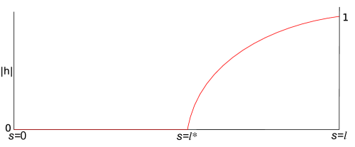
Suppose there exists a point conjugate to in . Consequently, there exists a non-null accessory extremal satisfying and . Let be a continuous arc defined as
and is depicted in Figure 1. The second variation along the arc is given by
However, this arc has a corner point at , as . If the matrix is positive definite, then by Weierstrass-Erdmann conditions Bolza (1904), the arc with a corner point cannot be the local minimizer. But, the second variation functional is zero along the present broken extremal . Therefore, there must exist another arc satisfying the boundary conditions (11) which is a local minimizer and further reduces the second variation , thereby proving the theorem.
∎
Therefore, these two conditions prove that the critical points correspond to local minima if they don’t have any conjugate points. Otherwise, they are not local minima.
3 Application to Cantilever structures
The main motivation for developing the conjugate point stability test is to determine the stability of tip-loaded soft cantilever arms. The deformations in the elastic rods are modelled using the standard Kirchhoff Rod theory Antman (2006), and we describe this theory in this section. Euler parameters are employed in our model to describe rotations and most of the notations adapted here are taken from Dichmann et al. (1996).
3.1 Kinematics and Equilibrium
The elastic rod configuration is modelled as an orientable curve in 3D space using a centreline and an orientation frame spanned by the orthonormal unit vectors called directors . The independent variable is the arclength of the undeformed configuration. The rate of change of the director frame with respect to the arclength is characterized using the Darboux vector as
| (19) |
Here, denotes the standard cross-product between two vectors. The components along the local directors , correspond to bending strains, while the component corresponds to twisting strain. We restrict ourselves to the case of inextensible and unshearable rods, where the tangent coincides with the tangent to the centreline
| (20) |
where denotes the differentiation with respect to arclength . We denote these local strain components using a triad . We consider the unstressed configuration or lowest energy configuration to be the reference state. Let be the triplet of strain components in its unstressed configuration. We also use the terms intrinsic shape or precurvature to denote these components. The orientation frame is connected to the fixed laboratory frame through an matrix, which is commonly parameterized using three Euler Angles. However, the three-dimensional representation of Euler angles does not completely represent the -space globally and has singular directions. The Euler parameters (or a Quaternion) Goldstein (1951); Shuster (1993) provides the global representation of space and mitigate the singularities. In addition, Euler parameters representation uses quadratic functions which are computationally quicker compared to the trigonometric functions used in Euler angle representation. The directors with respect to the fixed coordinate system can be written in terms of Euler parameters as
| (21) | ||||
Similarly, the strain components in terms of Euler parameters and their derivatives Dichmann et al. (1996) are given by
| (22) |
where , are skew symmetric matrices given by
| (23) |
These matrices map to vectors that are orthogonal to each other as well as orthogonal to .
The stresses acting along the cross-section of the rod can be averaged out to yield internal force and moment . The components are the bending moments and the component is the twisting moment in the rod. We use to denote the triad of these components . We consider the rods that satisfy Hyperelastic constitutive law. A convex strain energy density function , exists such that , and the moment components are given by
| (24) |
where the shifted strain argument describe the strain from intrinsic shape . In the present work, we restrict ourselves to a simple linearly elastic constitutive model where the strain energy density function is given by
| (25) |
the moment components are given by
| (26) |
Here, for are called bending stiffnesses or Flexural rigidity and is called torsional stiffness of the rod and is given by . Here is Young’s modulus of the material, is the second moment of area of the cross-section of the rod, and is the Poisson’s ratio of the material and its value is for an incompressible material. For a circular cross-section rod, , where is its cross-sectional radius.
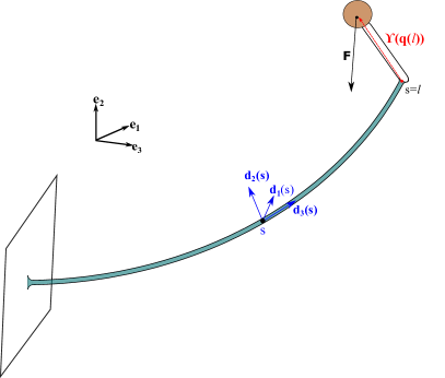
We consider a problem where a massless elastic rod is clamped at one end and a dead payload applied at the other end as shown in Figure 2. The payload is rigidly attached to the tip , and so its spatial orientation depends on the orientation frame of the tip , which is a function of , the Euler parameters at . The lever arm connecting the point of attachment and the point of application of force in the fixed frame is given by
| (27) |
where represents the components of the arm in the tip’s frame and represents this triad. The payload exerts a force and a moment at the tip . Here, denotes the standard cross-product between two vectors. Then, the stored potential energy due to this applied tip load is
The rod equilibria are the constrained critical points of the strain energy functional of the total energy functional, which is the sum of elastic strain energy and stored potential energy
| (28) |
subject to pointwise constraints
| (29) |
By definition, Euler parameters have a unit length . Instead of enforcing it, we choose it to enforce . This equation together with the boundary conditions is equivalent to . This constrained variational problem is formulated as an unconstrained variational problem using the Lagrange multipliers , . The functional represented by
| (30) |
is stationary at the equilibrium. We refer to the integrand as the Augmented Lagrangian. The Hamiltonian form of the equilibria Dichmann et al. (1996) is adapted here, as they offer more simplicity in terms of analysis and numerics. The phase variables in this Hamiltonian formulation are the states and their corresponding conjugate momenta , . The internal force and the impetus are defined using the Augmented Lagrangian as
| (31) |
The dot product of with fetches the components of the internal moment in terms of Hamiltonian variables
| (32) |
On the other hand, the dot-product of with gives the expression for the Lagrange multiplier . The Hamiltonian of the system after taking the Legendre transformation of appears as
| (33) |
Then, the canonical form of the Hamiltonian system of equations governing the equilibria is given by
| (34a) | ||||
| (34b) | ||||
| (34c) | ||||
| (34d) | ||||
where the derivative is
and the component are written in terms of phase variables and using the relation (32). These ODEs are subjected to fixed boundary conditions at
| (35) |
and Natural boundary conditions at the other end
| (36a) | ||||
| (36b) | ||||
| (36c) | ||||
The condition (36b) results from projection of Natural boundary conditions of onto -space and the other (36c) results from projection of it onto (For more details see (Dhanakoti, 2023, page 33-35)). The last expression (36c) can be set to any value as it specifies the Lagrange multiplier with a boundary condition and restricts its gauge freedom Li and Maddocks (1996). The quantity specifies the given orientation.
3.2 Stability Analysis
The equilibria obtained as the solutions to (34) with the boundary conditions (35), (36) must satisfy the Legendre’s strengthened condition (4) along with the Jacobi condition in order for it to represent the local minima of the functional (28). The variable has no explicit contribution in the elastic strain energy , and it acts only through boundary conditions and the constraint . We decouple and its conjugate momentum from the variational problem for stability analysis by directly substituting the relations in the functional to yield
| (37) |
The variations in and are represented using and respectively. In this analysis, we restrict the variations , which ensures the unit-norm constraint . As a result, satisfies or equivalently is orthogonal to . There are many choices of the basis for this orthogonal vectors , and we choose the basis for our computations. Any arbitrary variation can be projected on to the using the projections in where
As a result, the new projection of the second variation reads as
where
Along the projected directions, the Hessian matrix
| (38) |
is positive definite and satisfies Legendre’s condition, whereas alone is only positive semi-definite. The linearization of the Hamiltonian form of the equilibria (34) gives the Hamiltonian form of the Jacobi operator
| (39) |
where the Hessian matrices , , , are partial derivatives of with respect to respective arguments. By restricting the variations only to basis, we obtain the Hamiltonian version of in projected space on . The absence of conjugate points in the interval is the sufficient condition for the equilibria to be stable, the computation of which is outlined below. The boundary with the Natural boundary conditions, i.e., is chosen and ivp is solved towards the other end for a basis of initial values for .
and with initial values of that satisfy the linearized boundary condition (36b), (36c)
| (40a) | ||||
| (40b) | ||||
The algebraic system (40) is solved to obtain the respective values of the components .
The components corresponding to the IVP solution for th set of IVP are denoted as , . These four components are arranged as rows in the matrix along as
| (41) |
This matrix is projected onto space to yield a matrix. We call this matrix stability matrix. A point is called conjugate point of if the determinant of this stability matrix vanishes for any . Therefore, by Jacobi condition, if the equilibrium possesses a conjugate point computed through the above method, it is unstable. We must solve a -dimensional IVP of Jacobi equations to assess the stability of the equilibria determined by the -dimensional boundary value problem (BVP) (34), (35) and (36).
4 Numerical Examples
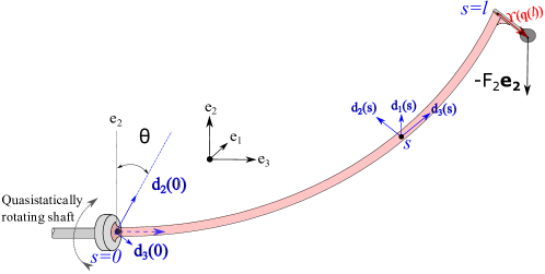
In this section, we deploy the proposed conjugate point test to deduce the stability of tip-loaded cantilever systems and investigate the potential occurrence of snap-back instability. Consider a naturally curved, slender, massless elastic rod clamped to a horizontal axis at one end and attached to a dead load at the other end, with gravity acting in a vertical direction as depicted in Figure 3. For all our examples, we choose the stiffness matrix as a diagonal matrix
| (42) |
and a downward acting vertical tip load . The clamped end is quasi-statically rotated about the horizontal tangent -axis by setting the boundary condition
| (43) |
and is numerically simulated by performing parameter continuation of (34) in using AUTO-07p Doedel et al. (2007). In this case, the system is periodic about , i.e., for any the system at and are identical.
4.1 Intrinsically Planar Curvatures
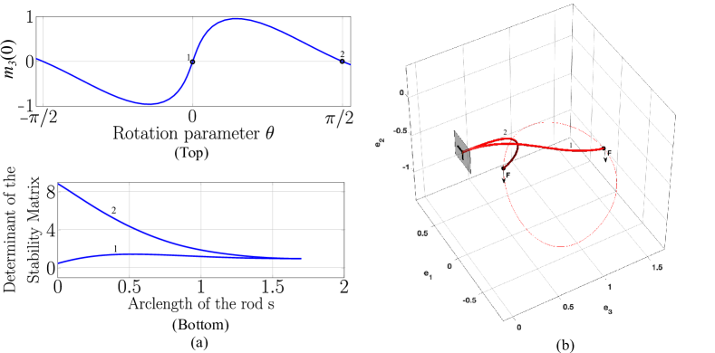
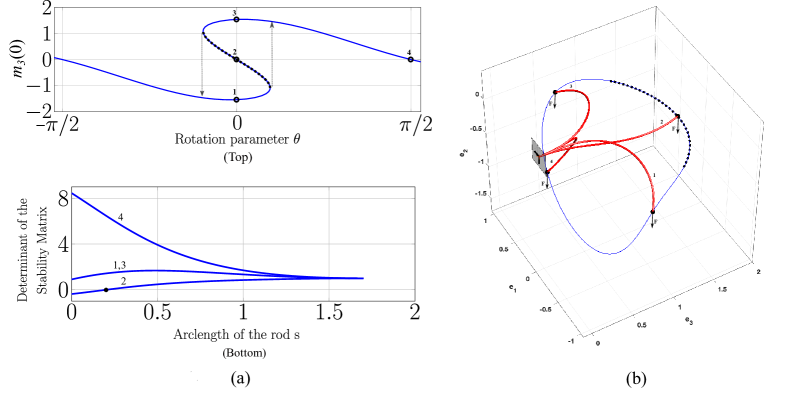
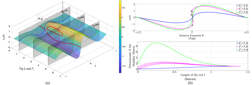
Initially, we analyze naturally planar rods with intrinsic curvature that have the form , subjected to a concentrated tip load . We quasi-statically rotate the clamped end by varying from to and observe the equilibria. This observation is continued for increasing values of , length and tip load . It is well known that if the rod is isotropic , the centrelines of the deformed configuration take the same shape for any rotation of the clamped end under a given non-zero tip load . However, if symmetry is broken by considering non-zero , the rod centrelines assume different forms for different values of under a given load . A few features of the equilibria from such a scenario are displayed in Figure 4 and 5, where the other parameters are set at and . At lower curvatures such as , the rod centrelines have a one-to-one mapping with respect to . The twist moment at the clamped end is evaluated from the continued solutions and is plotted against to fetch the bifurcation diagram. In our examples, corresponds to the rod shapes curving vertically upwards. The stability of these equilibria is assessed through conjugate point computations, as detailed in the prior section 3.2. All the equilibria are stable as they exhibit no conjugate points. A few computations for the labelled equilibria are displayed in Figure 4a (bottom). On the other hand, higher curvature such as , results in equilibria that violate the one-to-one mapping with respect to in the neighborhood of . In this region, three equilibria exist for an identical . In parameter continuation, these scenarios are characterized by folds in the parameter ( in the present case) as shown in Figure 5a (Top). Conjugate point tests reveal that two of these equilibria are stable, while the other (that lies between the folds) is unstable. The tip trace corresponding to unstable equilibria is denoted by black dotted lines, indicating a discontinuous path of stable solutions. Consequently, the configurations transition abruptly from one stable configuration to another when operated around this parameter space (around ), mimicking a catapult behavior. The dynamics of a rotating cantilever, as a consequence of this instability is out of the scope of this paper. Details regarding the snapping dynamics of planar naturally straight elastic rods can be found in Armanini et al. Armanini et al. (2017). Standard bifurcation theory Golubitsky and Schaeffer (2014) predicts that the folds in the bifurcation parameter are the points of stability exchange, and our conjugate point computations concur with it. The evolution of the rod configurations and the snap-back instability depends on their history in cases with folds, as denoted by the arrows in Figure 5a (Top). Therefore, we also use the term hysteresis to describe this phenomenon.
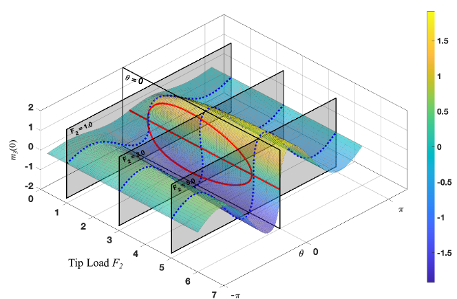
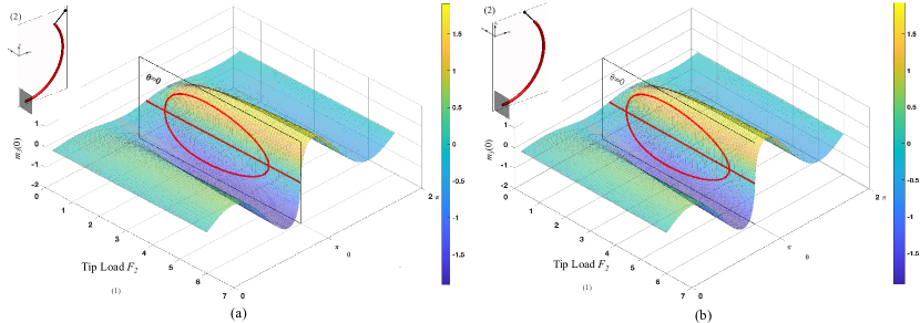
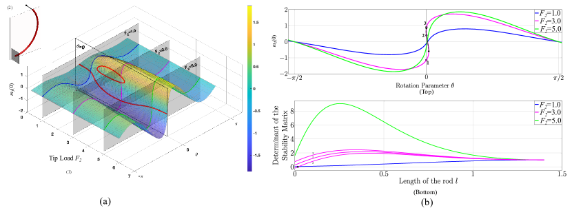
The nature and extent of the hysteresis region in cantilevers are governed by the complex interplay among the system parameters such as intrinsic curvature , length , and tip load , as illustrated in the following example. Consider a cantilever setup with intrinsic shape , length , subject to a concentrated tip load . Parameter continuation is performed along the clamp angle from to by incrementally increasing the value of from to . From the resulting solutions, bifurcation diagrams ( vs. plots) are generated for different values of and are plotted as a surface plot, as shown in Figure 6. This surface plot is referred to as a bifurcation surface. The planar bifurcation diagrams for , and are depicted by the corresponding planes slicing this surface. The curves corresponding to and have no region of unstable equilibria, whereas the diagram for has a region of unstable equilibria characterized by the presence of folds. Another orthogonal plane bisects this surface fetching a curve that can be interpreted as a Bifurcation diagram when the parameter is varied at fixed . The presence of two perfect pitchforks illustrates the symmetrical nature of the rod deformations around . This diagram indicates the rod’s response as the tip load is increased at a fixed that corresponds to the rod being planar and curving upwards. We draw here some preliminary conclusions, relying primarily on the plots and without extensive analysis. As the magnitude of tip load increases, the planar equilibrium of the rod, represented by a straight line, experiences two pitchfork bifurcations-the first one supercritical and the second one subcritical. According to Bifurcation theory, the trivial solution (which in the present context is planar rod equilibrium at ) loses stability at supercritical pitchfork bifurcation as it passes through and regains stability at the subcritical pitchfork bifurcation. The equilibria at which lies between the folds correspond to this unstable trivial line between the bifurcations.
To gain a better insight on dependence of hysteresis behavior on the system properties, we non-dimensionalize the quantities by substituting , , and leading to
| (44a) | ||||
| (44b) | ||||
where and are the associated system dimensionless parameters. In the present cantilever setup with intrinsic planar curvatures under a vertical concentrated tip load, the vector , where and the dimensionless intrinsic curvature . The boundary conditions are
| (45a) | |||
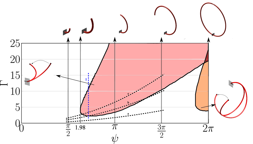
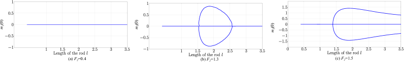
The other two governing equations (34a), (34b) are disregarded for non-dimensionalization in this part of the analysis as they do not influence the physics of the problem. The equation (34a) connects the position vector of the rod with quaternions while the term (34b) yields the constant value of internal force . The parameter indicates the scale of the cantilever system and the applied load, whereas represents the dimensionless curvature and is the angle formed by the arc at the centre. We perform the continuation in parameter of a complete rotation for different values of and and assess if the hysteresis region exists. Figure 7 depicts the space where the hysteresis region for a rotating cantilever exists. In this analysis, we restrict our consideration to values of up to , representing a complete circle turn, while neglecting any instances of self-contact. The unstable modes emerge only for values of . The shape of this diagram is influenced by the Poisson ratio of the material, which is set to an incompressible case of in the present case. The hysteresis region on the left side of the plot corresponds to the unstable equilibria that occur around , as indicated. On the other hand, the region on the right (in a different shade) corresponds to the unstable equilibria that occur around . There is a little portion on the top left, where unstable equilibria occur around both and . A key takeaway from this diagram is that it has areas where the hysteresis phenomenon can be manipulated by tuning the parameter either upwards or downwards. One example, discussed earlier in Figure 6, shows hysteresis can be tuned by increasing or decreasing the value of , and the path taken by this case of fixed is indicated by the vertical line I on the plot. Another control instance is by maintaining a fixed and tuning its length . To analyze this strategy, we plot the bifurcation diagrams obtained by the plane slicing the surface for different values of as shown in Figure 8. For smaller tip loads such as , there is no sign of hysteresis for any length . When increases to , hysteresis behavior appears for intermediate values of . Further rise of to leads to hysteresis behavior for all values of . These control paths take the form of parabolas as indicated by the dotted curves a,b and c in the plot in Figure 7. In conclusion, the tip load can be adjusted to obtain a closed hysteresis region, an open hysteresis region, or no hysteresis region. This selective range of values, for which hysteresis can be switched on or off, holds potential applications in the design of soft robot arms. From an engineering perspective, the parameters or can be externally manipulated. Another instance of control mechanism is through tuning intrinsic curvature, which is feasible in active elastic rods Kaczmarski et al. (2022, 2024).
4.2 Effect of Torsion Component or Arm of the Load
Let us examine the effect of the remaining parameters such as torsion component and load arm on the hysteresis behavior. These parameters may induce asymmetry in the system, potentially breaking the symmetry. Initially, we slightly tune the component from to a small non-zero value of , while keeping the other remaining parameters constant as in the prior case and perform the similar analysis of varying at increments of . The resulting bifurcation surface and features are displayed in Figure 9. The symmetric surface in Figure 6 transforms into a non-symmetric surface, clearly evident when the plane intersects it, revealing two disconnected, non-symmetric curves (in red), displayed in Figure 9a . The bifurcation diagrams corresponding to and have no folds, while the bifurcation diagram for has a fold. The equilibrium corresponding to positioned between the folds (labelled ) is unstable, as it has one conjugate point. This observation is the same as that of the previous case of in Figure 5a. However, the curves corresponding to from the conjugate point tests with labels and do not coincide here, as both these configurations are not exact mirror images about . Additionally, it is noticeable that the line is not precisely centered between the two folds, and the plot shifted slightly right compared to the previous case of in Figure 5a. This strategy of tuning torsion can be implemented in active elastic rods Kaczmarski et al. (2022, 2024).
Let us now focus on the load arm , which is a triad of three components and . The centrelines of an unstressed uniform rod with intrinsic curvature are planar and lie in the plane. Therefore, a non-zero value of or results in the arm lying in this plane. These two parameters generate bifurcation surfaces, as shown in Figure 10, which qualitatively resemble that in Figure 6 and indicate symmetric behavior about . However, the other component results in the arm non-planar with the undeformed rod, introducing asymmetry in the system, as demonstrated by its bifurcation surfaces corresponding to in Figure 11. A comparison between the cases of , , and is shown using the plots obtained by slicing the plane with bifurcation surfaces, as depicted in Figure 12. A positive component shrinks the band of hysteresis, while a negative component expands it. On the other hand, a positive shrinks the band, while its negative component expands it. From a technical perspective, a tunable arm with a varying can be easily designed and controlled so that snapping can be turned on or off. The asymmetry-inducing non-planar component inverts the bifurcation diagram for its negative component. Hence, load arm is capable of stabilizing or destabilizing the cantilever equilibria. In conclusion, the parameters and are capable of inducing the symmetry-breaking in the bifurcation surfaces, while the components and quantitatively vary the bifurcation surfaces without any qualitative effect.
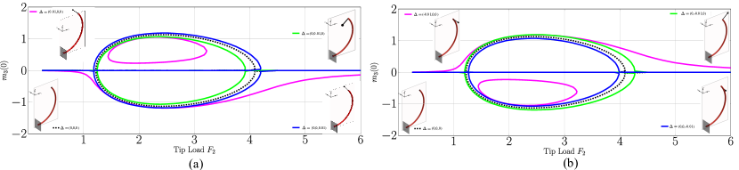
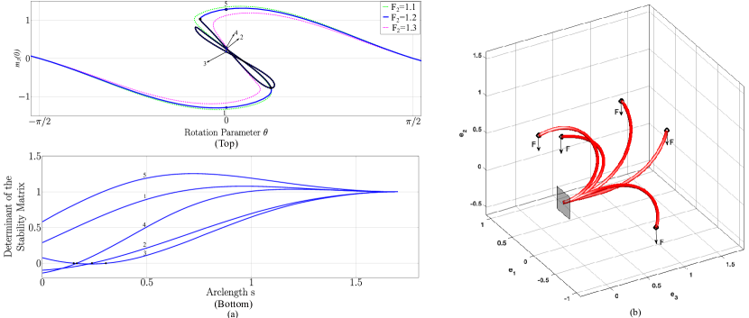
In our analysis, we have primarily focused on cases that exhibited either zero or one conjugate point. However, slightly higher values of or may result in equilibria with more than one conjugate point. For instance, let us increase the value of to and perform the continuation in for incrementing values of in range . The resulting bifurcation diagrams exhibit four folds for intermediate values of , as depicted in Figure 13a. The number of folds increases from two to four as increases from to and reduces back to two for further increase in to . The five equilibrium configurations corresponding to on a plot with four folds are depicted in Figure 13b, and their stability is assessed. Equilibrium labeled has two conjugate points, while the other equilibria, labeled and , each have one conjugate point, and all are unstable. The prediction that the presence of folds indicates the exchange of stability is, once again supported. Typically, near a fold, a stable equilibrium becomes unstable. However, an unstable equilibrium may either become stable or transition to a higher unstable mode (more than one conjugate point). In this example, we observe all possible stability transitions at the folds: from stable to unstable, from unstable to a higher unstable mode, back to a lower unstable mode, and then to stable at successive folds. Equilibria with zero conjugate points are stable and exist realistically. Therefore, the mere identification of folds is insufficient to analyze stability in these cases. Further details about the direction of stability transition are required, and conjugate point computations are more beneficial in this context.
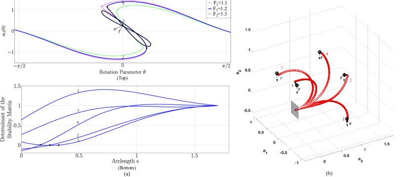
A similar qualitative behavior is observed when the arm parameter is increased to , and continuation is performed for different values of . The five equilibrium configurations for on the curve with four folds are displayed, and their stability is analyzed, as displayed in Figure 14. Both the torsion components and exhibit similar qualitative effects on the hysteresis behavior of the current cantilever system. Moreover, these two last examples in this section illustrate how tuning certain parameters drastically affects the nonlinear behavior of the cantilevers with intrinsic curvatures.
5 Summary and Discussion
The Jacobi condition has been generalized to study the critical points of variational problems with fixed-free ends. The literature concerning the necessary and sufficient conditions for this set of problems is relatively sparse. To address this, the definition of conjugate points is slightly modified. This theory was developed keeping in mind the applications relevant to rapidly advancing soft robots. The equilibria of tip-loaded cantilevers, which mimic flexible soft robotic arms, were computed through the Hamiltonian formulation, and their stability properties were analyzed by computing conjugate points. The Jacobi equations were shooted as IVPs from the free end towards the fixed end to compute conjugate points. The role of intrinsic curvature in generating the nonlinear behavior of elastic rods is particularly emphasized in the examples. A flexible intrinsically curved elastic rod is subjected to a quasi-static rotation at one end and a vertical tip load at the other. Depending on the system parameters, there are two possible outcomes: the tip either traces a smooth, continuous curve, or it traces a discontinuous curve due to intermediate unstable equilibria, leading to snap-back instability. Surprisingly, the hysteresis behavior displayed a complex dependence on the parameters of tip load, length, and intrinsic curvature. For example, the hysteresis behavior displayed non-monotonic characteristics for a certain combination of parameters. An initial increase in the tip load beyond a critical value led to the onset of hysteresis. But when the load increased past the second critical value, this hysteresis behavior vanished. The intricate relationship among the system parameters that govern the hysteresis was numerically represented through a plot using non-dimensional quantities. Furthermore, the impact of the load arm in stabilizing or destabilizing the rod equilibria was also discussed. These findings could be useful in designing innovative devices, which can be employed as switches or triggers. This investigation may be extended to the cases with distributed loads like gravity or electrostatics.
Generally, the folds that arise in continuation solutions indicate an exchange of stability. In all examples, the stability change at the folds aligned well with the conjugate point tests. Although, the direction of change is unknown, the - periodicity of the cantilever system in the rotation parameter, and the information of folds may aid in predicting the stability when there are just two folds. However, one solution along the continued solutions must be analyzed for stability and should correspond to the stable equilibrium to effectively implement this strategy. Moreover, the stability prediction based solely on the folds may fail when more than two folds occur consecutively, as seen in some examples. In these scenarios, stability can be determined only through the conjugate point tests. There have been several studies relating the number of conjugate points to the Morse index Manning et al. (1998); Hoffman et al. (2002), the maximal dimension of subspace over which the second variation is negative definite. The combination of Legendre’s strengthened condition, Sturm-Liouville problem, and Rayleigh quotients may allow this extension to the cases with fixed-free ends.
References
- Matsutani [2010] Shigeki Matsutani. Euler’s Elastica and Beyond. Journal of Geometry and Symmetry in Physics, 17(none):45 – 86, 2010. doi:10.7546/jgsp-17-2010-45-86.
- Manning et al. [1996] Robert S. Manning, John H. Maddocks, and Jason D. Kahn. A continuum rod model of sequence-dependent DNA structure. The Journal of Chemical Physics, 105(13):5626–5646, 10 1996. ISSN 0021-9606. doi:10.1063/1.472373.
- Park et al. [2019] Yunyoung Park, Yongsam Kim, and Sookkyung Lim. Locomotion of a single-flagellated bacterium. Journal of Fluid Mechanics, 859:586–612, 2019. doi:10.1017/jfm.2018.799.
- Singh et al. [2022] Raushan Singh, Abhishek Arora, and Ajeet Kumar. A computational framework to obtain nonlinearly elastic constitutive relations of special cosserat rods with surface energy. Computer Methods in Applied Mechanics and Engineering, 398:115256, 2022. ISSN 0045-7825. doi:https://doi.org/10.1016/j.cma.2022.115256.
- McMillen et al. [2002] Tyler McMillen, Alain Goriely, et al. Tendril perversion in intrinsically curved rods. Journal of Nonlinear Science, 12(3):241–281, 2002. doi:10.1007/s00332-002-0493-1.
- Miller et al. [2014] J. T. Miller, A. Lazarus, B. Audoly, and P. M. Reis. Shapes of a suspended curly hair. Phys. Rev. Lett., 112:068103, Feb 2014. doi:10.1103/PhysRevLett.112.068103.
- Hafner and Bickel [2021] Christian Hafner and Bernd Bickel. The design space of plane elastic curves. ACM Trans. Graph., 40(4), jul 2021. ISSN 0730-0301. doi:10.1145/3450626.3459800.
- Rucker et al. [2010] D. Caleb Rucker, III Robert J. Webster, Gregory S. Chirikjian, and Noah J. Cowan. Equilibrium conformations of concentric-tube continuum robots. The International Journal of Robotics Research, 29(10):1263–1280, 2010. doi:10.1177/0278364910367543. PMID: 25125773.
- Chen et al. [2020] Shoue Chen, Yunteng Cao, Morteza Sarparast, Hongyan Yuan, Lixin Dong, Xiaobo Tan, and Changyong Cao. Soft crawling robots: design, actuation, and locomotion. Advanced Materials Technologies, 5(2):1900837, 2020. doi:10.1002/admt.201900837.
- Laschi et al. [2012] Cecilia Laschi, Matteo Cianchetti, Barbara Mazzolai, Laura Margheri, Maurizio Follador, and Paolo Dario. Soft robot arm inspired by the octopus. Advanced Robotics, 26(7):709–727, 2012. doi:10.1163/156855312X626343.
- Majidi [2014] Carmel Majidi. Soft robotics: A perspective—current trends and prospects for the future. Soft Robotics, 1(1):5–11, 2014. doi:10.1089/soro.2013.0001.
- O’Reilly and Peters [2012] Oliver M. O’Reilly and Daniel M. Peters. Nonlinear stability criteria for tree-like structures composed of branched elastic rods. Proceedings of the Royal Society A: Mathematical, Physical and Engineering Sciences, 468(2137):206–226, 2012. doi:10.1098/rspa.2011.0291.
- Romero et al. [2021] Victor Romero, Mickaël Ly, Abdullah Haroon Rasheed, Raphaël Charrondière, Arnaud Lazarus, Sébastien Neukirch, and Florence Bertails-Descoubes. Physical validation of simulators in computer graphics: A new framework dedicated to slender elastic structures and frictional contact. ACM Transactions on Graphics (TOG), 40(4):1–19, 2021. doi:10.1145/3450626.3459931.
- Bolza [1904] Oskar Bolza. Lectures on the Calculus of Variations, volume 14. University of Chicago Press, 1904.
- Gelfand et al. [1963] Izrail Moiseevitch Gelfand, Richard A Silverman, et al. Calculus of variations. Courier Corporation, 1963.
- Maddocks [1984] J. H. Maddocks. Stability of nonlinearly elastic rods. Archive for Rational Mechanics and Analysis, 85(4):311–354, 1984. doi:10.1007/BF00275737.
- Manning et al. [1998] Robert S. Manning, Kathleen A. Rogers, and John H. Maddocks. Isoperimetric conjugate points with application to the stability of dna minicircles. Proceedings of the Royal Society of London. Series A: Mathematical, Physical and Engineering Sciences, 454(1980):3047–3074, 1998. doi:10.1098/rspa.1998.0291.
- Hoffman et al. [2002] Kathleen A. Hoffman, Robert S. Manning, and Randy C. Paffenroth. Calculation of the stability index in parameter-dependent calculus of variations problems: Buckling of a twisted elastic strut. SIAM Journal on Applied Dynamical Systems, 1(1):115–145, 2002. doi:10.1137/S1111111101396622.
- Manning [2009] Robert S. Manning. Conjugate points revisited and neumann–neumann problems. SIAM Review, 51(1):193–212, 2009. doi:10.1137/060668547.
- Kuznetsov and Levyakov [2002] V.V. Kuznetsov and S.V. Levyakov. Complete solution of the stability problem for elastica of euler’s column. International Journal of Non-Linear Mechanics, 37(6):1003–1009, 2002. ISSN 0020-7462. doi:https://doi.org/10.1016/S0020-7462(00)00114-1.
- Levyakov and Kuznetsov [2010] S. V. Levyakov and V. V. Kuznetsov. Stability analysis of planar equilibrium configurations of elastic rods subjected to end loads. Acta Mechanica, 211(1):73–87, 2010. doi:10.1007/s00707-009-0213-0.
- Goriely and Tabor [1997] Alain Goriely and Michael Tabor. Nonlinear dynamics of filaments i. dynamical instabilities. Physica D: Nonlinear Phenomena, 105(1-3):20–44, 1997. doi:10.1016/S0167-2789(96)00290-4.
- Kumar and Healey [2010] Ajeet Kumar and Timothy J Healey. A generalized computational approach to stability of static equilibria of nonlinearly elastic rods in the presence of constraints. Computer Methods in Applied Mechanics and Engineering, 199(25-28):1805–1815, 2010. doi:10.1016/j.cma.2010.02.007.
- Armanini et al. [2017] C. Armanini, F. Dal Corso, D. Misseroni, and D. Bigoni. From the elastica compass to the elastica catapult: an essay on the mechanics of soft robot arm. Proceedings of the Royal Society A: Mathematical, Physical and Engineering Sciences, 473(2198):20160870, 2017. doi:10.1098/rspa.2016.0870.
- Warner [1997] Jeremy A. Warner. Numerical simulations of elastic rods. Master’s thesis, University of Maryland, College Park, USA, 1997.
- Vetyukov and Oborin [2023] Yury Vetyukov and Evgenii Oborin. Snap-through instability during transmission of rotation by a flexible shaft with initial curvature. International Journal of Non-Linear Mechanics, 154:104431, 2023. ISSN 0020-7462. doi:10.1016/j.ijnonlinmec.2023.104431.
- Sipos and Várkonyi [2020] András A. Sipos and Péter L. Várkonyi. The longest soft robotic arm. International Journal of Non-Linear Mechanics, 119:103354, 2020. ISSN 0020-7462. doi:10.1016/j.ijnonlinmec.2019.103354.
- Antman [2006] S. Antman. Nonlinear Problems of Elasticity. Applied Mathematical Sciences. Springer New York, 2006.
- Dichmann et al. [1996] Donald J. Dichmann, Yiwei Li, and John H. Maddocks. Hamiltonian formulations and symmetries in rod mechanics. In Jill P. Mesirov, Klaus Schulten, and De Witt Sumners, editors, Mathematical Approaches to Biomolecular Structure and Dynamics, pages 71–113. Springer New York, New York, NY, 1996. doi:10.1007/978-1-4612-4066-2_6.
- Goldstein [1951] Herbert Goldstein. Classical Mechanics. Addison-Wesley Press, Inc, Massachusetts, 1951.
- Shuster [1993] Malcolm David Shuster. A survey of attitude representation. Journal of The Astronautical Sciences, 41:439–517, 1993.
- Dhanakoti [2023] Siva Prasad Chakri Dhanakoti. Study of Intrinsically Curved Elastic Rods Under External Loads with Applications to Concentric Tube Continuum Robots and their Control. PhD thesis, Freie Universität Berlin, 2023. URL https://refubium.fu-berlin.de/handle/fub188/42994.
- Li and Maddocks [1996] Y Li and J. H Maddocks. On the computation of equilibria of elastic rods part i:integrals, symmetry and a hamiltonian formulation. preprint, 1996.
- Doedel et al. [2007] Eusebius J Doedel, Alan R Champneys, Fabio Dercole, Thomas F Fairgrieve, Yu A Kuznetsov, B Oldeman, RC Paffenroth, B Sandstede, XJ Wang, and CH Zhang. Auto-07p: Continuation and bifurcation software for ordinary differential equations. 2007.
- Golubitsky and Schaeffer [2014] Martin Golubitsky and David G Schaeffer. Singularities and Groups in Bifurcation Theory. Springer, 2014.
- Kaczmarski et al. [2022] Bartosz Kaczmarski, Derek E. Moulton, Ellen Kuhl, and Alain Goriely. Active filaments i: Curvature and torsion generation. Journal of the Mechanics and Physics of Solids, 164:104918, 2022. ISSN 0022-5096. doi:10.1016/j.jmps.2022.104918.
- Kaczmarski et al. [2024] Bartosz Kaczmarski, Sophie Leanza, Renee Zhao, Ellen Kuhl, Derek E. Moulton, and Alain Goriely. Minimal design of the elephant trunk as an active filament. Phys. Rev. Lett., 132:248402, Jun 2024. doi:10.1103/PhysRevLett.132.248402.