Let Occ Flow: Self-Supervised
3D Occupancy Flow Prediction
Abstract
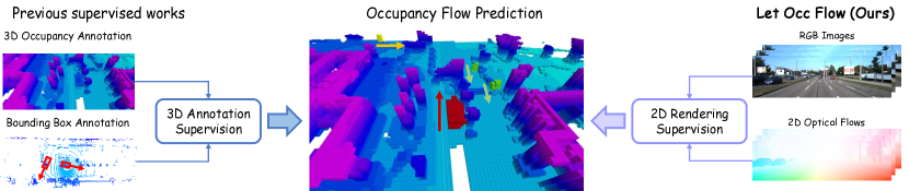
Accurate perception of the dynamic environment is a fundamental task for autonomous driving and robot systems. This paper introduces Let Occ Flow, the first self-supervised work for joint 3D occupancy and occupancy flow prediction using only camera inputs, eliminating the need for 3D annotations. Utilizing TPV for unified scene representation and deformable attention layers for feature aggregation, our approach incorporates a backward-forward temporal attention module to capture dynamic object dependencies, followed by a 3D refine module for fine-gained volumetric representation. Besides, our method extends differentiable rendering to 3D volumetric flow fields, leveraging zero-shot 2D segmentation and optical flow cues for dynamic decomposition and motion optimization. Extensive experiments on nuScenes and KITTI datasets demonstrate the competitive performance of our approach over prior state-of-the-art methods. Our project page is available at https://eliliu2233.github.io/letoccflow/.
Keywords: 3D occupancy prediction, occupancy flow, Neural Radiance Field
1 Introduction
Accurate perception of the surrounding environment is crucial in autonomous driving and robotics for downstream planning and action decisions. Recently, vision-based 3D object detection [1, 2] and occupancy prediction [3, 4, 5, 6, 7] have garnered significant attention due to their cost-effectiveness and robust capabilities. Building on these foundations, the concept of occupancy flow prediction has emerged to offer a comprehensive understanding of the dynamic environment by estimating the scene geometry and object motion within a unified framework [8, 9].
Existing occupancy flow prediciton methods [8, 9] rely heavily on detailed 3D occupancy flow annotations, which complicates their scalability to extensive training datasets. Previous research has attempted to address the dependency on 3D annotations for occupancy prediction tasks. Some strategies utilized LiDAR data to generate occupancy labels [3, 10, 11], but struggle to balance between accuracy and completeness due to LiDAR’s inherent sparsity and dynamic object movements. Recently, some methods have emerged to enable 3D occupancy predictions in a self-supervised manner by integrating the NeRF-style differentiable rendering with either weak 2D depth cues [7] or photometric supervision [5, 6]. However, existing self-supervised techniques take static world assumption as a premise and never consider the motion of foreground objects. This raises a question: Can we bridge 2D perception cues to enable self-supervised occupancy flow prediction?
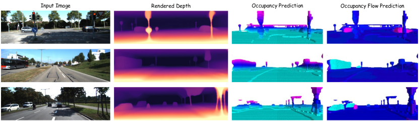
To address the aforementioned issues, we introduce Let Occ Flow, a novel method for simultaneously predicting 3D occupancy and occupancy flow using only camera input, without requiring any 3D annotations for supervision, as shown in Figure 1. Our approach employs Tri-perspective View(TPV) [11] as a unified scene representation and incorporates deformable attention layers to aggregate multi-view image features. For temporal sequence inputs, we utilize a BEV-based backward-forward attention module to effectively capture long-distance dependencies of dynamic objects. Subsequently, we use a 3D refine module for spatial volume feature aggregation and transform the scene representation into fine-grained volumetric fields of SDF and flow.
Differentiable rendering techniques are then applied to jointly optimize scene geometry and object motion. Specifically, for geometry optimization, we employ a photometric consistency supervision [6]. While LiDAR data is available, we employ range rendering supervision [12, 13] for efficient geometric-aware sampling and avoiding the occlusion caused by the extrinsic parameters between LiDAR and the camera sensors. For motion optimization, we leverage semantic and optical flow cues for dynamic decomposition and supervision. These cues are convenient to obtain from pre-trained 2D models, which have shown superior zero-shot generalization capability in comparison to 3D models. Furthermore, previous studies have demonstrated that self-supervised photometric consistency [14, 15] enables the pre-trained flow estimator to effectively narrow the generalization gap across different data domains. Specifically, we employ a pre-trained 2D open-vocabulary segmentation model GroundedSAM [16] to derive a segmentation mask of movable objects. In addition, we use optical flow cues from an off-the-shelf 2D estimator [17, 18] to offer effective supervision of pixel correspondence for joint geometry and motion optimization.
In summary, our main contributions are as follows:
1. We proposed Let Occ Flow, the first self-supervised method for jointly predicting 3D occupancy and occupancy flow, by integrating 2D optical flow cues into geometry and motion optimization.
2. We designed a novel temporal fusion module with BEV-based backward-forward attention for efficient temporal interaction. Furthermore, we proposed a two-stage optimization strategy and dynamic disentanglement scheme to mitigate the training instability and sample imbalance problem.
3. We conducted extensive experiments on various datasets with qualitative and quantitative analyses to show the competitive performance of our approach.
2 Related Work
2.1 3D Occupancy Prediction
Vision-centric 3D occupancy prediction has emerged as a promising method to perceive the surrounding environment. TPVFormer [11] introduces a tri-perspective view representation from multi-camera images. SurroundOcc [3] utilizes sparse LiDAR data to generate dense occupancy ground truth as supervision. Rather than using 3D labels, RenderOcc [7] employs volume rendering to enable occupancy prediction from weak 2D semantic and depth labels. Recently, SimpleOccupancy [4], OccNeRF [5], and SelfOcc [6] propose a LiDAR-free self-supervised manner by photometric consistency. Despite the progress in static occupancy prediction, there has been comparatively less focus on occupancy flow prediction—a critical component for dynamic planning and navigation in autonomous driving.
2.2 Neural Radiance Field
Reconstructing 3D scenes from 2D images remains a significant challenge in computer vision. Among the various approaches, Neural Radiance Field (NeRF)[19] has gained increasing popularity due to its strong representational ability. To enhance training efficiency and improve rendering quality, several methods[20, 21, 22] have adopted explicit voxel-based representations. Additionally, some approaches [23, 24] introduced NeRF into surface reconstruction by developing Signed Distance Function(SDF) representation. Further advancements [25, 26, 27, 28] have been made to facilitate scene-level sparse view reconstruction by conditioning NeRF on image features, laying the groundwork for generalizable NeRF architectures.
2.3 Scene Flow
Scene flow enables autonomous systems to perceive motion in highly dynamic environments by offering dense motion estimation for each point in the scene. FlowNet3D [29] introduced deep-learning to estimate scene flow when trained solely on synthetic data. NSFP [30] optimizes a neural network to estimate the scene flow with expensive per-timestep optimization. Unlike previous methods that estimate correspondence between two input frames, some approaches proposed to combine scene flow prediction with vision-based occupancy network [8, 9], while they rely heavily on complete 3D occupancy and flow annotations. Our proposed approach addresses this gap by being the first work to jointly predict 3D occupancy and occupancy flow in a self-supervised manner, establishing a new direction for future research in this field.
3 Method
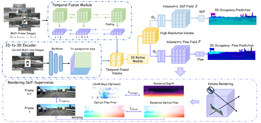
The overall framework is shown in Figure 2. In Sec.3.2, we first extract 3D volume features from multi-view temporal sequences with 2D-to-3D feature encoder. To capture the geometry and motion information, we employ an attention-based temporal fusion module and utilize a 3D refine module to ensure effective spatial-temporal interaction. Next in Sec.3.3, we construct the volumetric SDF and flow field using two MLP decoders and perform differentiable rendering to optimize the network with 2D labels in a self-supervised manner. Finally in Sec.3.4, we illustrate a flow-oriented two-stage training strategy and dynamic disentanglement scheme for joint geometry and motion optimization.
3.1 Problem Formulation
We aim to provide a unified framework for joint prediction of 3D occupancy and occupancy flow of the surrounding scenes at timestep using a temporal sequence of multi-view camera inputs. Formally, our prediction task is represented as:
| (1) |
where is a neural network, represents -view images at timestamp . denotes the 3D occupancy at timestamp , representing the occupied probability of each 3D volume grid with the value between 0 and 1. And denotes the occupancy flow at timestamp , representing the motion vector of each grid in the horizontal direction of 3D space.
3.2 2D-to-3D Encoder
2D-to-3D Feature Encoder. Following existing 3D occupancy methods [6, 11], we utilize TPV to effectively construct a unified representation from multi-view image input, which pre-define a set of queries in the three axis-aligned orthogonal planes:
| (2) |
where denote the resolution of the three planes and represents the feature dimension. We can integrate multi-view multi-scale image features extracted from the 2D encoder backbone [31] into triplane using deformable cross-attention [32] (DAttn) and feed forward network (FFN):
| (3) |
Then we construct a full-scale 3D feature volume by broadcasting each TPV plane along the corresponding orthogonal direction and aggregating them by summation up [11].
Temporal Fusion. To effectively capture temporal geometry and object motion, we design a temporal fusion module to enhance the scene representation further. Previous approaches [7, 33] utilize a residual block of convolution networks to fuse concatenated temporal volume features. However, it is hard for the convolution module to align the volume features of moving objects due to the inherent local receptive field. In contrast, the attention module has been proven to have the ability to capture long-distance dependencies [1]. Additionally, compared with voxel-based fusion, BEV-based temporal interaction is more computationally efficient without accuracy degradation [9].
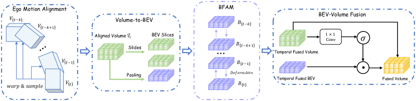
Specifically, our temporal fusion module integrates historical feature volume into the current frame. As depicted in Figure 3, this module comprises two main components: ego-motion alignment in voxel space and a Backward-Forward Attention Module (BFAM) in BEV space. To compensate for ego-motion, we first apply feature warping by transforming historical feature volumes to the current frame, according to the relative pose in ego coordinate:
| (4) |
where is the aligned feature volume in the current local ego coordinate. denotes the predefined reference points of current feature volume, is the ego pose transformation matrix from to , and indicates the linear interpolation operator.
Inspired by prior works [34, 35], we compress the aligned feature volume into a series of BEV slices along the z-axis and employ deformable attention [32] (DAttn) between these BEV slices in the horizontal direction. To effectively capture overall information in the vertical dimension, we derive a global BEV feature using an average pooling operator and integrate it into the BEV slices. Furthermore, we employ a Backward-Forward Attention Module (BFAM) to enhance the interaction between temporal BEV features:
| (5) |
where represents the BEV features at adjacent frames , and is a learnable scale factor. In the backward process, , while in the forward process, .
After BFAM, we recover the fused feature volume by merging fused BEV slices, and utilize the BEV-Volume Fusion module to achieve interaction between fused global BEV features and fused feature volume for the final feature volume :
| (6) |
where is a convolution module and is a sigmoid function.
3D Refine Module. Following the acquisition of the final fused feature volume , we utilize a residual 3D convolution network to further aggregate spatial features and subsequently upsample it to refined feature volume with high resolution using 3D deconvolutions.
3.3 Rendering-Based Optimization
Rendering Strategy. Given refined feature volume , we employ two separate MLP to construct volumetric SDF field and volumetric flow field :
| (7) |
During training, we employ a rendering-based strategy to concurrently optimize the 3D occupancy and occupancy flow without 3D annotations. Following [4, 6], we utilize SDF for geometric representation, with occlusion-aware rendering as NeuS[23]. Details are shown in the supplementary.
Rendering-Based Supervision. Inspired by [4, 5, 6, 25], we utilize a reprojection photometric loss for effective optimization of the volumetric SDF field:
| (8) |
where denotes the number of points sampled along the ray, is the sampled pixel on the current image, represents the transformation matrix from timestamp to in ego coordinate, and are the intrinsic and extrinsic parameters of cameras, respectively. Additionally, , , and denote the weight, depth, and flow of sampled point. For the photometric loss , we utilize the combination of L1 and D-SSIM loss, following monodepth [36].
Though photometric loss is sufficient for geometric supervision, optimizing object motion jointly remains a significant challenge. Therefore, we incorporate optical flow cues from an off-the-shelf flow estimator [17, 18] to offer an additional source of supervision for geometry and motion estimation.
| (9) |
where represents the estimated forward flow map from frame to .
When LiDAR is available, we could combine LiDAR supervision to enhance the geometry. Specifically, we first independently generate rays from the LiDAR measurement to ensure an effective sampling rate in regions with sufficient geometric observations, thereby avoiding occlusion problems from camera extrinsic. Furthermore, we implement a Scale-Invariant loss [37] between rendered ranges and LiDAR measurements to mitigate the global scene scale influence.
SDF Field Regularization. Due to the explicit physical interpretation of SDF representation, regularization can be effectively applied to the volumetric SDF field to prevent over-fitting with limited supervision. Initially, an eikonal term is employed for each sample point along camera and LiDAR rays to promote the establishment of a valid SDF field, where denotes the pre-computed gradient field of the volumetric SDF grid. Additionally, we also utilize a Hessian loss on the second-order derivatives of the SDF grid, following the approach of SelfOcc [6]. Furthermore, an edge-aware smoothness loss is employed following monodepth2 [36] to enforce neighborhood consistency of rendered depths and flows.
3.4 Flow-Oriented Optimization
Due to the training instability caused by the inherent ambiguities in jointly optimizing geometry and motion without ground truth labels, and the sample imbalance problem of moving objects and the static background, it becomes imperative to employ an effective flow-oriented optimization strategy.
Two Stage Optimization. To tackle the training instability challenge, we introduce a two-stage optimization strategy. Initially, we optimize the SDF field with the static assumption following the method proposed by SelfOcc [6] to generate a coarse geometric prediction. In the second stage, we jointly optimize the volumetric SDF and flow field with extra 2D optical flow supervision.
Dynamic Disentanglement. To effectively regularize the motion in static regions and solve the sample imbalance problem, we propose to conduct dynamic disentanglement using dynamic optical flow , which is subtracted by flow cues and static flow computed by rendered depth :
| (10) |
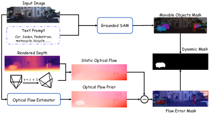
To mitigate incorrect decomposition caused by inaccurate depth estimation in background regions(eg.sky and thin structure), we leverage the zero-shot open-vocabulary 2D semantic segmentation model, Grounded-SAM [16], to extract binary masks for movable foreground objects. With flow error mask thresholded by dynamic flow , we could get an accurate dynamic mask for scene decomposition. Then we can regularize the volumetric flow field by minimizing the rendered flow map in static regions: .
Compared to the static background, dynamic objects such as cars or pedestrians account for a small proportion in driving scenes but hold significant importance for driving perception and planning. To address the imbalance caused by moving objects, we employ a scale factor to adjust the flow loss of dynamic rays based on their occurrence.
| (11) |
where and denote the static and dynamic parts of the flow loss calculated by Equation 9, while and represent the number of all sampled rays and dynamic rays, and is a threshold hyperparameter.
Static Flow Supervision. Since optical flow cues provide the pixel correspondence between adjacent frames, they could be used to supervise the scene geometry effectively. Specifically, we utilize the dynamic mask mentioned above to decouple the static regions and then leverage the forward static flow for geometry supervision. To effectively use the abundant training data in a self-supervised manner, we sample an auxiliary previous frame based on the Gaussian distribution of the distance between the ego coordinates to offer an additional backward flow for geometric supervision.
Finally, our overall loss function is summarized as follows:
| (12) |
4 Experimental Results
4.1 Self-supervised 3D Occupancy Prediction
We conduct experiments on 3D occupancy prediction using the SemanticKITTI [39] dataset without LiDAR supervision and employ RayIoU [40] as evaluation metrics. We also evaluate the results of monocular depth estimation using Abs Rel, Sq Rel, RMSE, RMSE log as metrics.
As reported in Table 1, our method sets the new state-of-the-art for 3D occupancy prediction and depth estimation tasks without any form of 3D supervision compared with other supervised and self-supervised approaches. Thanks to our effective spatial-temporal feature aggregation and the integration of optical flow cues for supervision, our method greatly enhances the geometric representation capabilities, compared to other rendering-based methods [5, 6, 25].
| Method | Occupancy | Depth | ||||||
|---|---|---|---|---|---|---|---|---|
| IoU@1 | IoU@2 | IoU@4 | RayIoU | Abs Rel | Sq Rel | RMSE | RMSE log | |
| MonoScene [41] | 26.00 | 36.50 | 49.09 | 37.19 | - | - | - | - |
| SceneRF [25] | 20.65 | 35.74 | 56.35 | 37.58 | 0.146 | 1.048 | 5.240 | 0.241 |
| OccNeRF [5] | 23.22 | 40.17 | 62.57 | 41.99 | 0.132 | 1.011 | 5.497 | 0.233 |
| SelfOcc [6] | 23.13 | 35.38 | 50.31 | 36.27 | 0.152 | 1.306 | 5.386 | 0.245 |
| Ours | 28.62 | 45.60 | 66.95 | 47.06 | 0.117 | 0.817 | 4.816 | 0.215 |
4.2 Self-supervised Occupancy Flow Prediction
We conduct occupancy flow prediction on the KITTI-MOT [38] and nuScenes [42] datasets. To compare with the OccNeRF* [5] and RenderOcc* [7], we add a concatenation&conv temporal fusion module and an occupancy flow head to the original model with extra 2D optical flow labels as supervision. To compare with OccNet [8], we use the official implementation to reproduce the results with GT 3D occupancy flow labels from OpenOcc [8] as supervision.
Due to the absence of occupancy flow annotations, we report the occupancy flow evaluation metrics on the KITTI-MOT dataset [38] using LiDAR-projected depths and generated flow labels. More details are presented in the supplementary materials. On the nuScenes [42] dataset, with annotated occupancy flow ground truth, we report the RayIOU [40] and mAVE metrics as OccNet [8].
| Method | Occupancy Flow | ||||||
|---|---|---|---|---|---|---|---|
| DE | EPE | DE_FG | EPE_FG | D1_5% | F1_10% | SF1_10% | |
| OccNeRF* [5] (w/o LiDAR) | 3.547 | 6.986 | 7.976 | 10.445 | 0.204 | 0.272 | 0.306 |
| Ours (w/o LiDAR) | 3.431 | 3.529 | 6.429 | 7.635 | 0.215 | 0.084 | 0.118 |
| OccNeRF* [5] (w/ LiDAR) | 2.667 | 8.131 | 4.040 | 11.284 | 0.137 | 0.309 | 0.326 |
| Ours (w/ LiDAR) | 2.610 | 3.488 | 3.106 | 7.510 | 0.154 | 0.083 | 0.105 |
| Method | Supervision | Occupancy Flow | |||||
| 3D | 2D | IOU@1 | IOU@2 | IOU@4 | RayIOU | mAVE | |
| OccNet [8] | 29.28 | 39.68 | 50.02 | 39.66 | 1.61 | ||
| OccNeRF* [5] | 16.62 | 29.25 | 49.17 | 31.68 | 1.59 | ||
| RenderOcc* [7] | 20.27 | 32.68 | 49.92 | 36.67 | 1.63 | ||
| Ours | 25.49 | 39.66 | 56.30 | 40.48 | 1.45 | ||
We report the results of occupancy flow prediction in Table 2 and Table 3. Compared to other rendering-based methods [5, 7], our approach performs much better on both KITTI-MOT [38] and nuScenes [42] dataset, owing to our effective temporal fusion module and flow-oriented optimization strategy. And compared with 3D supervised OccNet [8], our approach achieves comparable performance on nuScenes [42], validating the effectiveness of our self-supervised training paradigm.
4.3 Ablation Study
We systematically conduct comprehensive ablation analyses on the temporal fusion module, optimization strategy, and static flow supervision to validate the effectiveness of every component of our method. All experiments are trained for 16 epochs, and without LiDAR supervision by default.
| Temporal Fusion Module | DE | EPE | DE_FG | EPE_FG | D1_5% | F1_10% | SF1_10% | Params. |
|---|---|---|---|---|---|---|---|---|
| Concatenation&3D Conv. | 3.515 | 3.638 | 6.423 | 7.743 | 0.223 | 0.090 | 0.126 | 11.39M |
| BEV Pool&Forward Attn. | 3.600 | 3.763 | 6.339 | 7.971 | 0.228 | 0.091 | 0.124 | 5.21M |
| Ours | 3.431 | 3.529 | 6.429 | 7.635 | 0.215 | 0.084 | 0.118 | 6.62M |
| Two Stage Optimization | Dynamic Disentanglement | DE | EPE | DE_FG | EPE_FG | D1_5% | F1_10% | SF1_10% |
|---|---|---|---|---|---|---|---|---|
| 3.760 | 4.403 | 4.194 | 8.853 | 0.258 | 0.121 | 0.152 | ||
| 3.064 | 3.633 | 3.600 | 7.966 | 0.191 | 0.089 | 0.114 | ||
| 2.610 | 3.488 | 3.106 | 7.510 | 0.154 | 0.083 | 0.105 |
| Backward Static Flow Supervision | Forward Static Flow Supervision | DE | EPE | DE_FG | EPE_FG | D1_5% | F1_10% | SF1_10% |
|---|---|---|---|---|---|---|---|---|
| 6.715 | 4.128 | 6.598 | 8.160 | 0.239 | 0.099 | 0.149 | ||
| 3.495 | 3.614 | 6.510 | 7.987 | 0.217 | 0.084 | 0.123 | ||
| 3.431 | 3.529 | 6.429 | 7.635 | 0.215 | 0.084 | 0.118 |
Temporal Fusion. We report the results of different temporal fusion settings in Table 4. Our proposed method achieves the best results. Compared to the 3D Convolution module, our method achieves better performance with lower memory cost due to our effective BEV-based backward-forward attention mechanism and the efficient temporal interaction between adjacent frames, rather than relying on global 3D convolution. Additionally, Our method effectively incorporates local and global information on the height dimension compared to the BEV-only attention module.
Optimization Strategy. We investigate the effect of our optimization strategy in Table 5. It is shown that both two-stage optimization and dynamic disentanglement scheme benefit mitigating the impact of the ambiguities for joint optimization of scene geometry and object motion.
Static Flow Supervision. We verify the effectiveness of static flow supervision in Table 6. As reported, extra pixel correspondence priors from forward and backward static flow can effectively improve the quality of scene geometry, thus making occupancy flow better.
5 Conclusion
In this study, we introduced Let Occ Flow, the first self-supervised method for joint 3D occupancy and occupancy flow prediction using only camera input. Utilizing the effective temporal fusion module and flow-oriented optimization, our approach effectively captures dynamic object dependencies, thus enhancing both scene geometry and object motion. Furthermore, our method extends the differentiable rendering to the volumetric flow field and leverages 2D flow and semantic cues for dynamic disentanglement. Consequently, our work paves the way for future research into more efficient and accurate self-supervised learning frameworks in dynamic environment perception.
Supplementary Material
Our supplementary material includes dataset details, implementation details, evaluation metrics, and additional visualization results.
Appendix A Dataset Details
The SemanticKITTI [39] dataset is a large-scale dataset based on the KITTI Vision Benchmark [38], which includes automotive LiDAR scans voxelized into 256 × 256 × 32 grids with 0.2m resolution for 22 sequences. The dataset contains 28 classes with non-moving and moving objects. In our experiments, we only use RGB images captured by cam2 as input from the KITTI odometry benchmark and follow the official split of the dataset, with sequence 08 for validation and other sequences from 0 to 10 for training.
The KITTI-MOT [38] dataset is based on the KITTI Multi-Object Tracking Evaluation 2012, which consists of 21 training sequences and 29 test sequences. It holds stereo images from two forward-facing cameras and LiDAR point clouds. We selected all the training sequences except sequences where the ego-car is stationary or contains only a small number of moving objects(sequence 0012, 0013, and 0017) for training, and select testing sequences 0000-0014 for validation. We also apply LiDAR data and pseudo-optical flow to coarsely select dynamic frames for a higher sampling rate in our training process.
The nuScenes [42] dataset consists of 1000 sequences of various driving scenes of 20 seconds duration each and the keyframes are annotated at 2Hz. Each sample includes RGB images collected by 6 surround cameras with horizontal FOV and LiDAR point clouds from 32-beam LiDAR sensors. The 1000 scenes are officially divided into training, validation, and test splits with 700, 150, and 150 scenes, respectively.
Appendix B Implementation Details
B.1 Model Architecture
We adopted ConvNeXt-Base with SparK [43] pretraining as the 2D image backbone and a four-level FPN [44] to extract image features. We utilize TPV [11] uniformly divided to represent a cuboid area for multi-view feature integration, i.e. [80, 80, 6.4] meters around the ego car for nuScenes [42] and [51.2, 51.2, 6.4] meters in front of the ego car for SemanticKITTI [39] and KITTI-MOT [38]. Considering the computational cost of the subsequent temporal fusion module, we use half of the output occupancy resolution for TPV grid cell, i.e. 0.8 meters for nuScenes and 0.4 meters for SemanticKITTI and KITTI-MOT, respectively.
For the input temporal sequence, we utilize 2 previous frames for our temporal fusion module. Our 3D refine module includes a three-layer residual 3D convolution block and a 3D FPN block for spatial feature integration. To upsample the volume into the output occupancy resolution, we use a deconvolution module as FBOCC [33]. We adopt separate two-layer MLPs as decoders to construct volumetric fields for SDF and flow.
B.2 2D Flow Estimation
For occupancy flow prediction in KITTI-MOT [38] dataset, we leverage the flow estimation model of Unimatch [17] trained on FlyingChairs [45], FlyingThings3D [46] and fine-tuned on KITTI [38] to predict optical flow maps for supervision directly. Note that the Unimatch model is trained in a supervised manner, we provide an unsupervised flow fine-tuning strategy following [47] when adapted to different driving scenes. Specifically, we fine-tune the Unimatch model utilizing unsupervised flow techniques including stopping the gradient at the occlusion mask, encouraging smoothness before upsampling the flow field, and continual self-supervision with image resizing.
As for the nuScenes [42] dataset, the 3D occupancy flow ground-truth data is only available at 2Hz keyframes so it is challenging for optical flow estimation. Thus we employed a tracking-based flow estimation strategy using CoTrackerV2 [18]. We aim to obtain accurate optical flow between two keyframes by including the non-keyframe sequences to capture the long-term track. Specifically, we first use open-vocabulary 2D segmentor GroundedSAM[16] to predict dynamic foreground semantic segmentation. Then we take the adjacent keyframes and the non-keyframe sequences between the two keyframes as video input and conduct dense track to capture the long-term motion dependency in the masked regions. Once we have the initial pixel coordinates in the first keyframe and the corresponding pixel coordinates in the next, we subtract the two and get the final optical flow map in the masked regions. We take this optical flow map with the dynamic foreground mask as pseudo-flow labels for occupancy flow prediction.
B.3 Training Settings
The resolution of the input image is 512x1408 for nuScenes [42], 352x1216 for SemanticKITTI [39], and 352x1216 for KITTI-MOT [38]. For loss weight, we set , if present, and the weights for the edge and the LiDAR losses are 0.02 and 0.2 respectively. During training, we adopt the AdamW optimizer with an initial learning rate 1e-4 and weight decay of 0.01. We use the multi-step learning rate scheduler with linear warming up in the first 1k iterations. We train our models with a total batch size of 8 on 8 A100 GPUs for 16 epochs. Experiments on SemanticKITTI [39] and KITTI-MOT [38] take less than one day, while experiments on nuScenes [42] finish within two days.
B.4 Temporal Fusion Module
Algorithm 1 provides the pseudo-code of our proposed temporal fusion module. In the BEV fusion process, we employ a Backward Forward Attention Module (BFAM) with deformable attention (DAttn) to fuse the BEV features from two adjacent frames. To illustrate our algorithmic process clearly, we visually demonstrate our temporal fusion module in the demo video.
B.5 Differentiable Rendering
In the rendering stage, we conduct a uniform sampling of points along the ray and apply a tri-linear interpolation operation to efficiently compute the SDF values for each point from the volumetric SDF field [22]. Furthermore, the unbiased rendering weights can be calculated by , with denoting the opacity value proposed by NeuS [23]:
| (13) |
where is sigmoid function with a temperature coefficient .
Let and denote the depth and flow of the i-th point, we can calculate the rendered depth and flow of the ray by:
| (14) |
Appendix C Evaluation Metrics
C.1 Depth Estimation Evaluation Metrics
Following [48, 49, 50], we use evaluation metrics for self-supervised depth estimation as follows:
| (15) |
| (16) |
where and indicate predicted and ground truth depths respectively, and indicates all pixels on the depth map. We calculate metrics for depth values in the range of [0.1, 80] meters using 1:2 resolution against the raw image.
C.2 3D Occupancy Prediction Evaluation Metrics
Previous approaches [6, 25, 41] utilize the intersection over union (IoU) as the evaluation metrics of 3D occupancy prediction on SemanticKITTI [39] dataset. However, according to our experiment results, the penalty is overly strict in evaluating the reconstruction quality effectively. As illustrated in Figure 6, we observed that rendering-based methods [6, 25] often generate true positive (TP) predictions(marked in green in the figure) distributed on the ground or in invisible regions below the ground. This prevents effective evaluation of reconstruction details, as a deviation of one voxel will lead to an IoU of zero. Furthermore, rendering-based methods tend to predict a thick surface due to the absence of supervision in invisible regions, causing a large number of false positive (FP) predictions(marked in red in the figure) and a significant reduction of the precision metric.
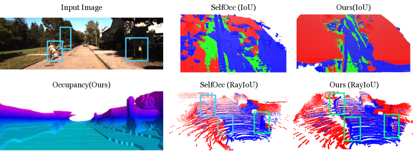
To demonstrate the advanced occupancy prediction quality of our approach, we employ Ray-based IoU (RayIoU) [40] as our evaluation metric and re-evaluate other comparative methods using their open-source checkpoint models. Initially, we generated LiDAR rays with origins sampled from the sequence, and then compute the travel distances of each LiDAR ray before intersecting with the occupied voxels. A query ray is classified as true positive(TP) when the L1 error between the predicted depth and ground-truth depth is less than a pre-defined threshold (1m, 2m, and 4m).
As is shown in Figure 6, the RayIoU metric reflected the superiority of our method on the detailed prediction of the tree and bicycles compared to SelfOcc.
C.3 Occupancy Flow Prediction Evaluation Metrics
On the KITTI-MOT [38] data, due to the absence of ground-truth occupancy flow labels, we conduct the evaluation following the scene flow benchmark of KITTI dataset [38]. Specifically, we use LiDAR-projected depth and pseudo 2D optical flow cues to generate disparity and optical flow labels. And we computed end-point error of rendered and ground-truth disparity (DE) and optical flow (EPE). D1_5% represent the percentage of disparity outliers with end-point error smaller than 4 pixels or 5% of the ground-truth disparity. F1_10% is the percentage of optical flow outliers with end-point error smaller than 8 pixels or 10% of the ground-truth flow labels. And SF_10% is the percentage of scene flow outliers (outliers in either D1_10% or F1_10%). To better evaluate the scene flow in foreground regions, we also reported the foreground disparity error (DE_FG) and optical flow error (EPE_FG) by leveraging the semantic mask obtained from GroundedSAM [16].
On the nuScenes [42] dataset, since we have the ground-truth occupancy flow labels, we use Ray-based IoU (RayIoU), and absolute velocity error (mAVE) for occupancy flow, following the evaluation metrics of Occupancy and Flow track for CVPR 2024 Autonomous Grand Challenge.
For RayIoU measurement, we perform evaluation on the OpenOcc benchmark [8] as introduced in subsection C.2. We use mAVE to indicate the velocity errors for a set of true positives (TP) with a threshold of 2m distance. The absolute velocity error (AVE) is defined for 8 classes (’car’, ’truck’, ’trailer’, ’bus’, ’construction_vehicle’, ’bicycle’, ’motorcycle’, ’pedestrian’) in m/s.
Appendix D Visualization Results
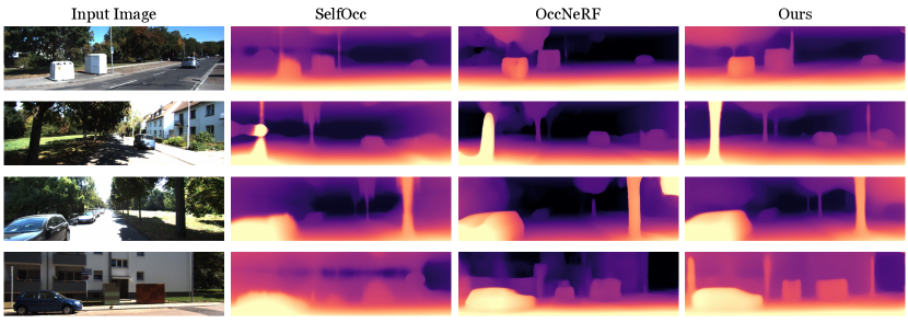
D.1 Depth Estimation
D.2 3D Occupancy Prediction
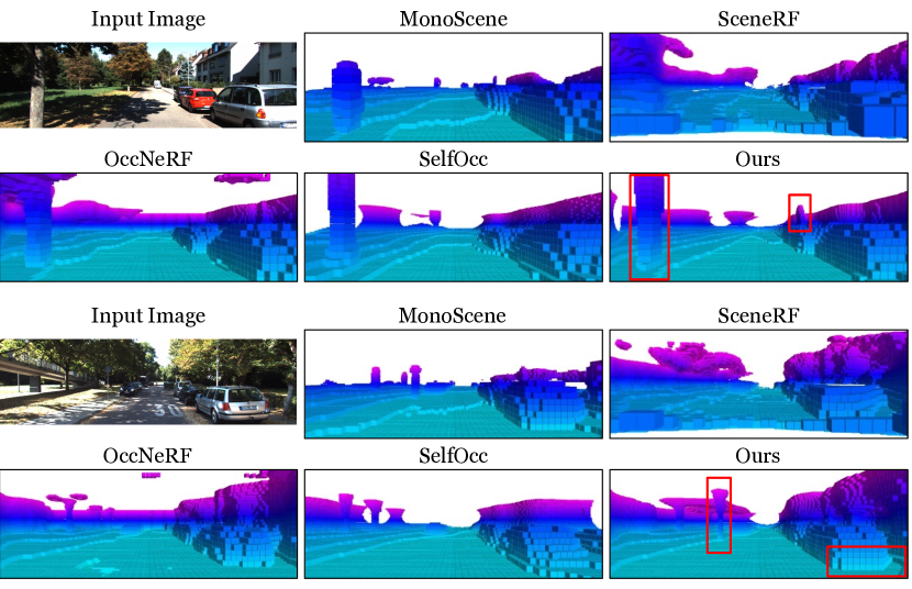
Figure 8 shows the qualitive comparison of 3D occupancy prediction on the SemanticKITTI [39] validation set. Our method achieves precise occupancy prediction for thin structures such as poles, trees, and cyclists. Also, it provides smooth predictions for cars and road surfaces compared to other supervised [41] and self-supervised [25, 5, 6] methods.
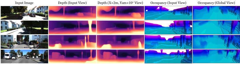
We provided more visualization results of depth estimation, novel view depth synthesis, and 3D occupancy prediction to illustrate the superiority of our method. As is shown in Figure 9, our method exhibited strong performance across these three tasks.
D.3 Occupancy Flow Prediction
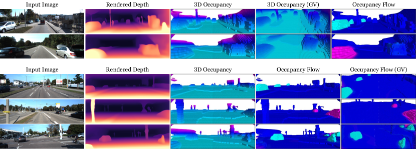
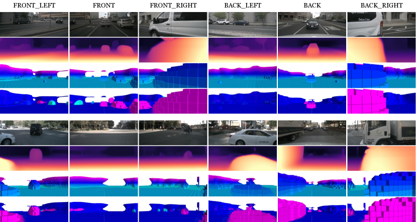
Figure 10 and Figure 11 shows the visualization results of the depth estimation and occupancy flow prediction tasks on the KITTI-MOT [38] and nuScenes [42] validation set. Our proposed method can simultaneously provide accurate 3D occupancy and occupancy flow prediction.
Appendix E Limitations and Future Work
Although we use temporal sequence input to better exploit the historical information, our model cannot completely handle the occlusion problem due to the inherent rendering-based limitation. Subsequent research could investigate long-term occupancy flow modeling and solutions to leverage the temporal sequence supervision to scale up the visible range of perspective. In addition, although our Let Occ Flow can offer accurate 3D occupancy and occupancy flow prediction, the prediction quality highly relies on the quality of optical flow cues, which serves as the supervision for the flow field. To improve the quality of 2D optical flow labels, we proposed a tracking-based flow estimation method and an unsupervised flow fine-tuning strategy. We hope the future work can pay more attention on the improvement of the flow supervision quality. Finally, our occupancy flow prediction does not explicitly enforce consistency within instances, and future work may explore to integrate instance perception into occupancy flow prediction.
References
- Li et al. [2022a] Z. Li, W. Wang, H. Li, E. Xie, C. Sima, T. Lu, Y. Qiao, and J. Dai. Bevformer: Learning bird’s-eye-view representation from multi-camera images via spatiotemporal transformers. arXiv preprint arXiv:2203.17270, 2022a.
- Li et al. [2022b] Y. Li, Z. Ge, G. Yu, J. Yang, Z. Wang, Y. Shi, J. Sun, and Z. Li. Bevdepth: Acquisition of reliable depth for multi-view 3d object detection. arXiv preprint arXiv:2206.10092, 2022b.
- Wei et al. [2023] Y. Wei, L. Zhao, W. Zheng, Z. Zhu, J. Zhou, and J. Lu. Surroundocc: Multi-camera 3d occupancy prediction for autonomous driving. arXiv preprint arXiv:2303.09551, 2023.
- Gan et al. [2023] W. Gan, N. Mo, H. Xu, and N. Yokoya. A simple attempt for 3d occupancy estimation in autonomous driving. arXiv preprint arXiv:2303.10076, 2023.
- Zhang et al. [2023] C. Zhang, J. Yan, Y. Wei, J. Li, L. Liu, Y. Tang, Y. Duan, and J. Lu. Occnerf: Advancing 3d occupancy prediction in lidar-free environments. arXiv preprint arXiv:2312.09243, 2023.
- Huang et al. [2023] Y. Huang, W. Zheng, B. Zhang, J. Zhou, and J. Lu. Selfocc: Self-supervised vision-based 3d occupancy prediction. arXiv preprint arXiv:2311.12754, 2023.
- Pan et al. [2023] M. Pan, J. Liu, R. Zhang, P. Huang, X. Li, L. Liu, and S. Zhang. Renderocc: Vision-centric 3d occupancy prediction with 2d rendering supervision. arXiv preprint arXiv:2309.09502, 2023.
- Tong et al. [2023] W. Tong, C. Sima, T. Wang, L. Chen, S. Wu, H. Deng, Y. Gu, L. Lu, P. Luo, D. Lin, et al. Scene as occupancy. In Proceedings of the IEEE/CVF International Conference on Computer Vision, pages 8406–8415, 2023.
- Li et al. [2024] J. Li, X. He, C. Zhou, X. Cheng, Y. Wen, and D. Zhang. Viewformer: Exploring spatiotemporal modeling for multi-view 3d occupancy perception via view-guided transformers. arXiv preprint arXiv:2405.04299, 2024.
- Chen Min,Xinli Xu,Dawei Zhao,Liang Xiao,Yiming Nie and Bin Dai [2023] Chen Min,Xinli Xu,Dawei Zhao,Liang Xiao,Yiming Nie and Bin Dai. Occ-bev: Multi-camera unified pre-training via 3d scene reconstruction. arXiv preprint, 2023.
- Huang et al. [2023] Y. Huang, W. Zheng, Y. Zhang, J. Zhou, and J. Lu. Tri-perspective view for vision-based 3d semantic occupancy prediction. arXiv preprint arXiv:2302.07817, 2023.
- Yang et al. [2023a] Z. Yang, Y. Chen, J. Wang, S. Manivasagam, W.-C. Ma, A. J. Yang, and R. Urtasun. Unisim: A neural closed-loop sensor simulator. In CVPR, 2023a.
- Yang et al. [2023b] J. Yang, B. Ivanovic, O. Litany, X. Weng, S. W. Kim, B. Li, T. Che, D. Xu, S. Fidler, M. Pavone, and Y. Wang. Emernerf: Emergent spatial-temporal scene decomposition via self-supervision. arXiv preprint arXiv:2311.02077, 2023b.
- Jonschkowski et al. [2020] R. Jonschkowski, A. Stone, J. T. Barron, A. Gordon, K. Konolige, and A. Angelova. What matters in unsupervised optical flow. In Computer Vision–ECCV 2020: 16th European Conference, Glasgow, UK, August 23–28, 2020, Proceedings, Part II 16, pages 557–572. Springer, 2020.
- Mao et al. [2024] Y. Mao, B. Shen, Y. Yang, K. Wang, R. Xiong, Y. Liao, and Y. Wang. -dba: Neural implicit dense bundle adjustment enables image-only driving scene reconstruction, 2024.
- Ren et al. [2024] T. Ren, S. Liu, A. Zeng, J. Lin, K. Li, H. Cao, J. Chen, X. Huang, Y. Chen, F. Yan, et al. Grounded sam: Assembling open-world models for diverse visual tasks. arXiv preprint arXiv:2401.14159, 2024.
- Xu et al. [2023] H. Xu, J. Zhang, J. Cai, H. Rezatofighi, F. Yu, D. Tao, and A. Geiger. Unifying flow, stereo and depth estimation. IEEE Transactions on Pattern Analysis and Machine Intelligence, 2023.
- Karaev et al. [2023] N. Karaev, I. Rocco, B. Graham, N. Neverova, A. Vedaldi, and C. Rupprecht. Cotracker: It is better to track together. arXiv:2307.07635, 2023.
- Mildenhall et al. [2021] B. Mildenhall, P. P. Srinivasan, M. Tancik, J. T. Barron, R. Ramamoorthi, and R. Ng. Nerf: Representing scenes as neural radiance fields for view synthesis. Communications of the ACM, 65(1):99–106, 2021.
- Fridovich-Keil et al. [2022] S. Fridovich-Keil, A. Yu, M. Tancik, Q. Chen, B. Recht, and A. Kanazawa. Plenoxels: Radiance fields without neural networks. In Proceedings of the IEEE/CVF Conference on Computer Vision and Pattern Recognition, pages 5501–5510, 2022.
- Müller et al. [2022] T. Müller, A. Evans, C. Schied, and A. Keller. Instant neural graphics primitives with a multiresolution hash encoding. ACM transactions on graphics (TOG), 41(4):1–15, 2022.
- Sun et al. [2022] C. Sun, M. Sun, and H. Chen. Direct voxel grid optimization: Super-fast convergence for radiance fields reconstruction. In CVPR, 2022.
- Wang et al. [2021] P. Wang, L. Liu, Y. Liu, C. Theobalt, T. Komura, and W. Wang. Neus: Learning neural implicit surfaces by volume rendering for multi-view reconstruction. arXiv preprint arXiv:2106.10689, 2021.
- Liang et al. [2022] R. Liang, J. Zhang, H. Li, C. Yang, Y. Guan, and N. Vijaykumar. Spidr: Sdf-based neural point fields for illumination and deformation. arXiv preprint arXiv:2210.08398, 2022.
- Cao and de Charette [2023] A.-Q. Cao and R. de Charette. Scenerf: Self-supervised monocular 3d scene reconstruction with radiance fields. In Proceedings of the IEEE/CVF International Conference on Computer Vision, pages 9387–9398, 2023.
- Wimbauer et al. [2023] F. Wimbauer, N. Yang, C. Rupprecht, and D. Cremers. Behind the scenes: Density fields for single view reconstruction. In Proceedings of the IEEE/CVF Conference on Computer Vision and Pattern Recognition, pages 9076–9086, 2023.
- Charatan et al. [2023] D. Charatan, S. Li, A. Tagliasacchi, and V. Sitzmann. pixelsplat: 3d gaussian splats from image pairs for scalable generalizable 3d reconstruction. arXiv preprint arXiv:2312.12337, 2023.
- Chen et al. [2024] Y. Chen, H. Xu, C. Zheng, B. Zhuang, M. Pollefeys, A. Geiger, T.-J. Cham, and J. Cai. Mvsplat: Efficient 3d gaussian splatting from sparse multi-view images. arXiv preprint arXiv:2403.14627, 2024.
- Liu et al. [2019] X. Liu, C. R. Qi, and L. J. Guibas. Flownet3d: Learning scene flow in 3d point clouds. In Proceedings of the IEEE/CVF conference on computer vision and pattern recognition, pages 529–537, 2019.
- Li et al. [2021] X. Li, J. Kaesemodel Pontes, and S. Lucey. Neural scene flow prior. Advances in Neural Information Processing Systems, 34:7838–7851, 2021.
- Liu et al. [2022] Z. Liu, H. Mao, C.-Y. Wu, C. Feichtenhofer, T. Darrell, and S. Xie. A convnet for the 2020s. In Proceedings of the IEEE/CVF conference on computer vision and pattern recognition, pages 11976–11986, 2022.
- Xia et al. [2022] Z. Xia, X. Pan, S. Song, L. E. Li, and G. Huang. Vision transformer with deformable attention. In Proceedings of the IEEE/CVF conference on computer vision and pattern recognition, pages 4794–4803, 2022.
- Li et al. [2023] Z. Li, Z. Yu, D. Austin, M. Fang, S. Lan, J. Kautz, and J. M. Alvarez. FB-OCC: 3D occupancy prediction based on forward-backward view transformation. arXiv:2307.01492, 2023.
- Zhang et al. [2023] Y. Zhang, Z. Zhu, and D. Du. Occformer: Dual-path transformer for vision-based 3d semantic occupancy prediction. arXiv preprint arXiv:2304.05316, 2023.
- Xia et al. [2024] Z. Xia, Z. Lin, X. Wang, Y. Wang, Y. Xing, S. Qi, N. Dong, and M.-H. Yang. Henet: Hybrid encoding for end-to-end multi-task 3d perception from multi-view cameras. arXiv preprint arXiv:2404.02517, 2024.
- Godard et al. [2019] C. Godard, O. Mac Aodha, M. Firman, and G. J. Brostow. Digging into self-supervised monocular depth prediction. October 2019.
- Eigen et al. [2014] D. Eigen, C. Puhrsch, and R. Fergus. Depth map prediction from a single image using a multi-scale deep network. Advances in neural information processing systems, 27, 2014.
- Geiger et al. [2012] A. Geiger, P. Lenz, and R. Urtasun. Are we ready for autonomous driving? the kitti vision benchmark suite. In 2012 IEEE conference on computer vision and pattern recognition, pages 3354–3361. IEEE, 2012.
- Behley et al. [2019] J. Behley, M. Garbade, A. Milioto, J. Quenzel, S. Behnke, C. Stachniss, and J. Gall. Semantickitti: A dataset for semantic scene understanding of lidar sequences. In Proceedings of the IEEE/CVF international conference on computer vision, pages 9297–9307, 2019.
- Liu et al. [2024] H. Liu, Y. Chen, H. Wang, Z. Yang, T. Li, J. Zeng, L. Chen, H. Li, and L. Wang. Fully sparse 3d occupancy prediction. arXiv preprint arXiv:2312.17118, 2024.
- Cao and De Charette [2022] A.-Q. Cao and R. De Charette. Monoscene: Monocular 3d semantic scene completion. In Proceedings of the IEEE/CVF Conference on Computer Vision and Pattern Recognition, pages 3991–4001, 2022.
- Caesar et al. [2020] H. Caesar, V. Bankiti, A. H. Lang, S. Vora, V. E. Liong, Q. Xu, A. Krishnan, Y. Pan, G. Baldan, and O. Beijbom. nuscenes: A multimodal dataset for autonomous driving. In Proceedings of the IEEE/CVF conference on computer vision and pattern recognition, pages 11621–11631, 2020.
- Tian et al. [2023] K. Tian, Y. Jiang, Q. Diao, C. Lin, L. Wang, and Z. Yuan. Designing bert for convolutional networks: Sparse and hierarchical masked modeling. arXiv preprint arXiv:2301.03580, 2023.
- Lin et al. [2017] T.-Y. Lin, P. Dollár, R. Girshick, K. He, B. Hariharan, and S. Belongie. Feature pyramid networks for object detection, 2017.
- Dosovitskiy et al. [2015] A. Dosovitskiy, P. Fischer, E. Ilg, P. Hausser, C. Hazirbas, V. Golkov, P. Van Der Smagt, D. Cremers, and T. Brox. Flownet: Learning optical flow with convolutional networks. In Proceedings of the IEEE international conference on computer vision, pages 2758–2766, 2015.
- Mayer et al. [2016] N. Mayer, E. Ilg, P. Hausser, P. Fischer, D. Cremers, A. Dosovitskiy, and T. Brox. A large dataset to train convolutional networks for disparity, optical flow, and scene flow estimation. In Proceedings of the IEEE conference on computer vision and pattern recognition, pages 4040–4048, 2016.
- Jonschkowski et al. [2020] R. Jonschkowski, A. Stone, J. T. Barron, A. Gordon, K. Konolige, and A. Angelova. What matters in unsupervised optical flow. In Computer Vision–ECCV 2020: 16th European Conference, Glasgow, UK, August 23–28, 2020, Proceedings, Part II 16, pages 557–572. Springer, 2020.
- Godard et al. [2019] C. Godard, O. Mac Aodha, M. Firman, and G. J. Brostow. Digging into self-supervised monocular depth estimation. In Proceedings of the IEEE/CVF international conference on computer vision, pages 3828–3838, 2019.
- Wei et al. [2023] Y. Wei, L. Zhao, W. Zheng, Z. Zhu, Y. Rao, G. Huang, J. Lu, and J. Zhou. Surrounddepth: Entangling surrounding views for self-supervised multi-camera depth estimation. In Conference on Robot Learning, pages 539–549. PMLR, 2023.
- Zhou et al. [2017] T. Zhou, M. Brown, N. Snavely, and D. G. Lowe. Unsupervised learning of depth and ego-motion from video. In Proceedings of the IEEE conference on computer vision and pattern recognition, pages 1851–1858, 2017.