July 25, 2024
Differential Effects of Sequence-Local versus Nonlocal
Charge Patterns on Phase Separation and
Conformational Dimensions of Polyampholytes as
Model Intrinsically Disordered Proteins
Tanmoy PAL,1,† Jonas WESSÉN,1,† Suman DAS,1,2,† and Hue Sun CHAN1,∗
1Department of Biochemistry, University of Toronto, Toronto, Ontario M5S 1A8, Canada
2Department of Chemistry, Gandhi Institute of Technology and Management, Visakhapatnam, Andhra Pradesh 530045, India
To appear in "J. Phys. Chem. Lett."
†Contributed equally.
∗Correspondence information:
Hue Sun CHAN.
E-mail: huesun.chan@utoronto.ca
Tel: (416)978-2697; Fax: (416)978-8548
Department of Biochemistry, University of Toronto,
Medical Sciences Building – 5th Fl.,
1 King’s College Circle, Toronto, Ontario M5S 1A8, Canada.
Abstract
Conformational properties of intrinsically disordered proteins (IDPs) are
governed by a sequence-ensemble relationship. To differentiate the impact of
sequence-local versus sequence-nonlocal features of an IDP’s charge pattern on
its conformational dimensions and its phase-separation propensity, the charge
“blockiness” and the nonlocality-weighted sequence charge
decoration (SCD)
parameters are compared for their correlations with isolated-chain radii of
gyration (s) and upper critical solution temperatures (UCSTs) of
polyampholytes modeled by random phase approximation, field-theoretic
simulation, and coarse-grained molecular dynamics. SCD is superior to
in predicting because SCD accounts for effects
of contact order, i.e., nonlocality, on dimensions of isolated chains.
In contrast, and SCD are
comparably good, though nonideal, predictors of UCST because frequencies of
interchain contacts in the multiple-chain condensed phase are less
sensitive to sequence
positions than frequencies of intrachain contacts of an isolated chain, as
reflected by correlating better with condensed-phase interaction
energy than SCD.
Extensive recent research has elucidated myriad
properties of biomolecular condensates
and their essential roles in diverse biological
functions (reviewed, e.g., in refs. (1; 2)).
These membraneless compartments are underpinned to
a significant degree by liquid-liquid phase separation (LLPS)
of intrinsically disordered proteins (IDPs), though more complex thermodynamic
processes such as gelation/percolation and dynamic mechanisms—involving
not only IDPs but folded protein domains as well as nucleic acids—also
contribute prominently.PappuChemRev ; Mingjie2023 ; HXZhouRev2024
The propensity for an IDP to undergo LLPS is dependent upon its sequence of
amino acids.Nott15 ; linPRL ; TanjaRohitNatChem2022
Many IDPs are enriched in charged and aromatic residues. Accordingly,
beside -related interactions,robert ; Chen2015 ; bauer2022 ; koby2023
electrostatics is an important driving force for many aspects of IDP
properties, as exemplified by its notable roles in IDP conformational
dimensions,rohit2013 ; kings2015 the stability of biomolecular
condensates,Nott15 ; knowles2022 and
a condensate’s capability to selectively recruit IDPs with
different sequence charge patterns.Sabari2023
An IDP can exist and function as essentially isolated
chain molecules and/or collectively in a multiple-chain condensate, or
certain intermediate oligomeric configurations in between. With this in mind,
analyzing the relationship between the behaviors of
isolated and condensed IDPs is instrumental not only for inferring
condensed-phase properties from those of computationally and experimentally
simpler isolated-chain systems. More fundamentally, it offers
insights into how sequence-encoded IDP properties are modulated
by IDP concentration.
For homopolymers with short-spatial-range interactions, it has been
known since the 1950s via the Flory-Huggins (FH) theory that the radius
of gyration of an isolated polymer anticorrelates with
the polymer’s LLPS propensity. This is because
decreases monotonically with the FH
interaction parameterFlory1951 at a given absolute temperature
and the LLPS critical
temperatureFlory1952
increases with when the interactions are purely enthalpic, i.e.,
and thus
where
and is polymer chain
length,KnowlesJPCL as is verified by recent simulations and more
sophisticated polymer theories.Panag1998 ; WangWang2014
Inspired by recent interest in sequence-specific IDP LLPS, similar
relationships for heteropolymers are
predicted between LLPS propensity and isolated-chain
(ref. (22)), coil-globule transition,BestPNAS2018
and two-chain association in a dilute
solution.Alan Likewise, dilute-phase and demixing
temperature was seen to correlate experimentally for
variants of the P domain of core stress-granule marker polyA-binding
protein undergoing heat-induced LLPS.Riback2017
The predicted dilute/condensed-phase correlations for heteropolymers
are significant but not perfect,lin2017 ; BestPNAS2018
as underscored by a recent
extensive simulation study of the human proteome.KrestenbioRxiv2024
The imperfection is instructive about the physical chemistry of
concentration-dependent IDP interactions.
We focus here on electrostatics as a first step.
Building on the substantial
recent works on polyampholyte configurations and
LLPS,rohit2013 ; kings2015 ; lin2017 ; joanJPCL2019 ; joanPNAS ; Wessen2021 ; Pal2021
we attend to a hitherto less explored consequence of sequence specificity,
namely how the impact of sequence-local patterns involving
charges proximate to one another differs from that of
sequence-nonlocal patterns encompassing charges far apart along the chain.
The differing effects of local versus nonlocal interactions has long
been recognized
in globular proteins. These include folding stabilityDill1990 and the
effects of intrachain contact orderChanDill1990 on conformational
ensembles as well as folding
kinetics.Dilletal1993 ; Plaxco1998 ; Chan98 ; AnnuRevPhysChem2011
But much about the corresponding effects for IDPs remains to be elucidated.
To make progress, here we contrast the predictive powers of two common
sequence charge parameters, namely the “blockiness” measure
(ref. (13)) and “sequence charge decoration”
(SCD, ref. (14)).
For a -bead polyampholyte with charge sequence
(),
captures primarily sequence-local aspects of the charge pattern
as its terms account for charge asymmetry
only in blocks of or consecutive beads relative to the
overall charge asymmetry of the polyampholyte in the form of
(refs. (13; 37)).
In contrast,
takes into account nonlocal sequence charge pattern
as it accords higher weights for
sequence-nonlocal pairs of charges.kings2015
Following several seminal
studies,rohit2013 ; kings2015 ; lin2017 ; joanJPCL2019
we consider overall-neutral polyampholytes with
(in units of the protonic charge) and
. Substantiating a preliminary
analysis,suman2 we rigorously determine the joint distribution
among all such sequences by
first estimating
the populated region in the -plane
via a diversity-enhanced genetic algorithmCamargoMolinaMandal2018
and then obtaining in the identified region using a
Wang-Landau approachWangLandau2001 (all SCD ;Alan see
text and Fig. S1a of Supporting Information for details).
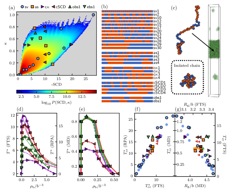
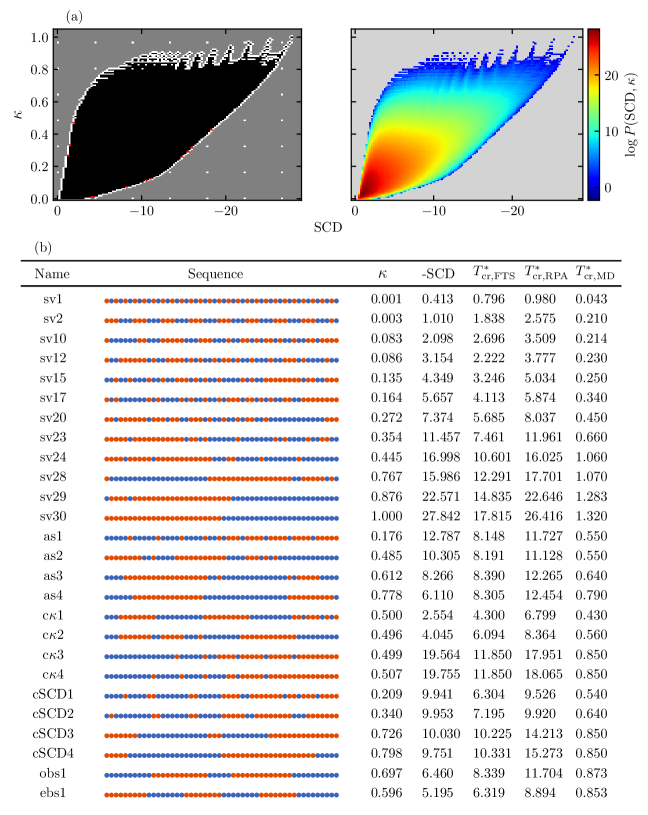
The resulting heat map for
in Fig. 1a exhibits a moderate correlation
between and (Pearson
correlation coefficient ).
Among these 50mers, we select for further analysis
26 sequences with a broad
coverage in Fig. 1a and are illustrative of
sequence variations of interest (Fig. 1b).
Beside the 12 “sv” sequences as examples of the
30 original sv sequencesrohit2013 are the
4 “as” sequences as controls for their –
anticorrelation opposing the overall positive
correlation.suman2 To probe the differential effects of
sequence-local versus nonlocal charge patterns, we construct
4 “c” sequences with diverse SCDs but essentially
the same , and
4 “cSCD” sequences with diverse s but essentially
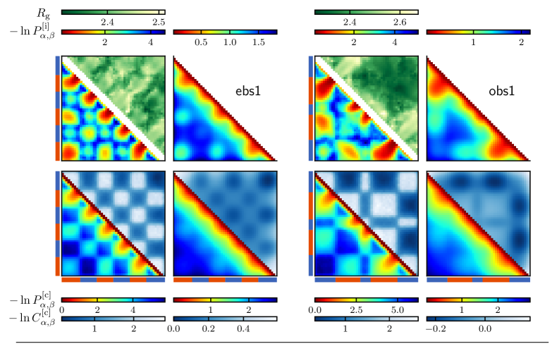
the same SCD. We also consider sequences obs1 and ebs1
with odd and even numbers of charge blocks, respectively, to assess
effects of like versus opposite charges at the two chain ends.
These sequences and their and SCD values are listed
in Table S1 and Fig. S1b of Supporting Information and marked in Fig. 1a.
By focusing on this set of sequences with the same chain length,
we address sequence charge
patterns’ impact on the thermodynamics of polyampholytes.
As such, further investigations of dynamic and other material
properties,koby2020 ; MittalNatComm2024 ; Wingreen2024
broader questions about sequence specificity for IDPs of different
chain lengths,RuffMiMB2021 ; PappuJMB2021
polyampholytes in high salt,kings2018
and for sequences
containing short spatial range hydrophobic-like
interactionsmoleculargrammar ; Zheng2020 ; WessenDasPalChan2022 ; Mittal2023 ; MittalNatChem2024
and/or with high net chargeskings2020 ; Caprin1_arXiv
are left to future studies.
Theories and computational models are available
to address sequence-specific LLPS of polyampholytes
(see, e.g., refs. (53; 54; 55; 56; 57), reviewed in ref. (58)).
Here we apply three complementary
methods: analytical random phase
approximation (RPA),Mahdi2000 ; Ermoshkin2003
field-theoretic simulation
(FTS),joanPNAS ; Parisi1983 ; Klauder1983 ; Fredrickson2006
and coarse-grained molecular dynamics (MD)
with the “slab” sampling method for
phase equilibriaPanagiotopoulos_Scaling_2017
(formulations described in Supporting Information), which
have afforded numerous physical
insights.linPRL ; joanJPCL2019 ; dignon18 ; Pal2021 ; WessenDasPalChan2022
Based on the same path-integral polymer model,
FTS is more accurate than RPA in principle because it
does not require an approximation like RPA and can be
extended to tackle nonelectrostatic interactions.WessenDasPalChan2022
Nonetheless, FTS is limited by finite resolution, simulation box size,
and treatments of excluded volume.joanJPCL2019 ; Pal2021
Compared to RPA and FTS, coarse-grained MD accounts better for structural
and energetic features of
IDPsZheng2020 ; Mittal2023 ; SumanPNAS ; Mpipi ; Kresten2021
but is computationally more costly.
To focus on electrostatics,
we adopt the “hard-core repulsion” MD
model with no nonelectrostatic attraction.suman2
The utility of combining the complementary advantages of RPA, FTS, and MD
is illustrated by recent studies of the dielectric
properties of condensatesWessen2021 and the effects
of salt and ATP on condensed polyampholytic and polyelectrolytic
biomolecules.Caprin1_arXiv
We employ all three methods for LLPS. s and pairwise bead-bead contacts—which are not amenable to RPA currently—are computed by MD and the following FTS approach: In a multiple-chain system, the root-mean-square radius of gyration of the th polymer , where denotes Boltzmann averaging, is the position of the th bead along the chain, and is the position ()-dependent bead center density. Since the correlation function that depends on the relative distance is amenable to FTS,Pal2021
| (1) |
where system volume , can now be computed by FTS. Similarly, with a generalized correlation between the th bead of the th chain and the th bead of the th chain,
| (2) |
is seen as the frequency of contact between the two beads, i.e., when
their centers are within a small distance (chosen here as where
is the reference bond length between sequentially consecutive beads).
Thus, through appropriate choices of and , intrachain contacts of
an isolated chain as well as intrachain and interchain contacts in the
condensed phase (Fig. 1c) can be computed by FTS via
.
A derivation of this formulation
based on the general FTS approachFredrickson2006 ; FredricksonGanesanDrolet2002 ; RigglemanRajeevFredrickson2012 ; MiMB2023
is provided in the Supporting Information.
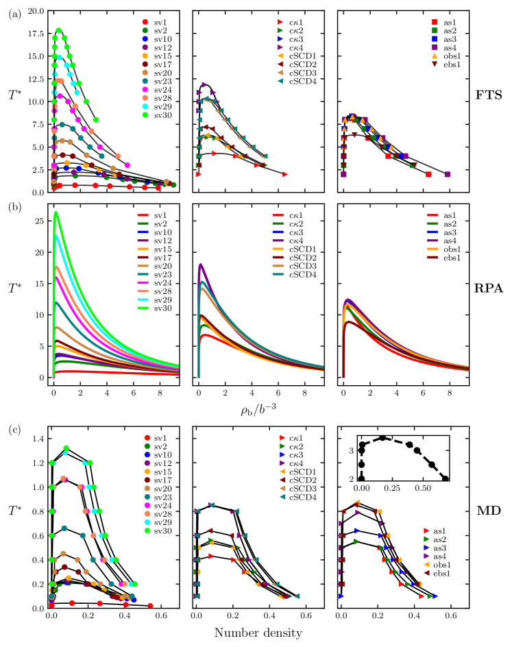
As examples, Fig. 1d,e show the RPA, FTS, and MD phase diagrams for
six sequences. Phase diagrams for all 26 sequences
in Fig. 1b are provided in Fig. S2 of
the Supporting Information. To facilitate comparisons,
temperatures are given as reduced temperature
where is Bjerrum length. Because of the
models’ different effective energy scales arising
from various approximations and treatments of
excluded volume, the critical temperatures, s,
predicted by RPA, FTS, and MD can be substantially
different for the same sequence
(Fig. S1b in Supporting Information). Nonetheless, the variation
in predicted by the models are well
correlated (Fig. 1f, Pearson correlation
coefficients ), indicating that the models are capturing
essentially the same sequence-dependent trend of LLPS propensity.
As to the relationship between and -dependent
root-mean-square isolated-chain , a sufficiently high for
a large sequence-dependent variation in is chosen for each
of the models in Fig. 1g.
Consistent with an earlier study on sv sequences,lin2017
s of isolated polyampholytes are well
correlated with their s in all three models (Fig. 1g).
Notably, however, there is an appreciable –
scatter in the MD model involving the cSCD, c, obs1, and ebs1
sequences which as a group is less conformative
to the moderate SCD– correlation than the sv sequences (Fig. 1a).
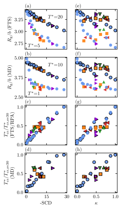
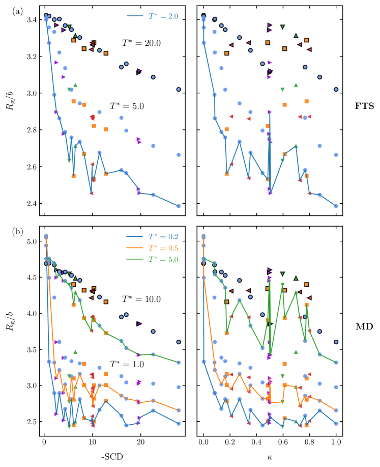
The impact of sequence-local versus nonlocal charge pattern on
and is assessed by comparing the extent to which
they are (anti)correlated with and SCD (Fig. 2).
depends on . Since the charge-pattern-dependent variation
in among sequences with moderate to high SCD values
is small at low as they adopt conformations with
similarly high compactness, two s are chosen for each of the FTS
and MD models in Fig. 2a,b,e,f with the higher producing ample
variations across the entire ranges of SCD and .
Corresponding data for additional s are provided in Fig. S3
of Supporting Information.
It is clear from Fig. 2a,b,e,f that anticorrelates
significantly better with SCD than .
For the sv sequences, anticorrelates reasonably well with
both SCD and . Indeed, the significant –
scatter seen in both FTS and MD (Fig. 2e,f) involves the as, cSCD, and
c sequences we introduced.
Despite the large variations in among the as and cSCD
sequences, their s are very similar.
For the c sequences, despite their essentially identical ,
their s are very different.
By comparison, the excellent SCD– anticorrelation is maintained
when challenged by these sequences (Fig. 1a,b).
In this light, the good – anticorrelation observed
previously for the sv sequencesrohit2013 is largely attributable
to the good correlation between the values of this particular
set of sv sequences and their SCDs.
In contrast to and SCD’s clearly different performance
for (which is the original target of both
parametersrohit2013 ; kings2015 , neither of these parameters was
derived originally for multiple-chain properties), their correlations
with are more comparable (Fig. 2c,d,g,h).
Unlike the excellent SCD– anticorrelation,
both the SCD– and –
correlations are good but not excellent.
While SCD is better than with
for RPA and FTS (Fig. 2c,g), is slightly better
for MD (Fig. 2d,h). Notably, for all
three models—RPA, FTS, and MD—the variation in is
larger among the c than among the cSCD sequences.
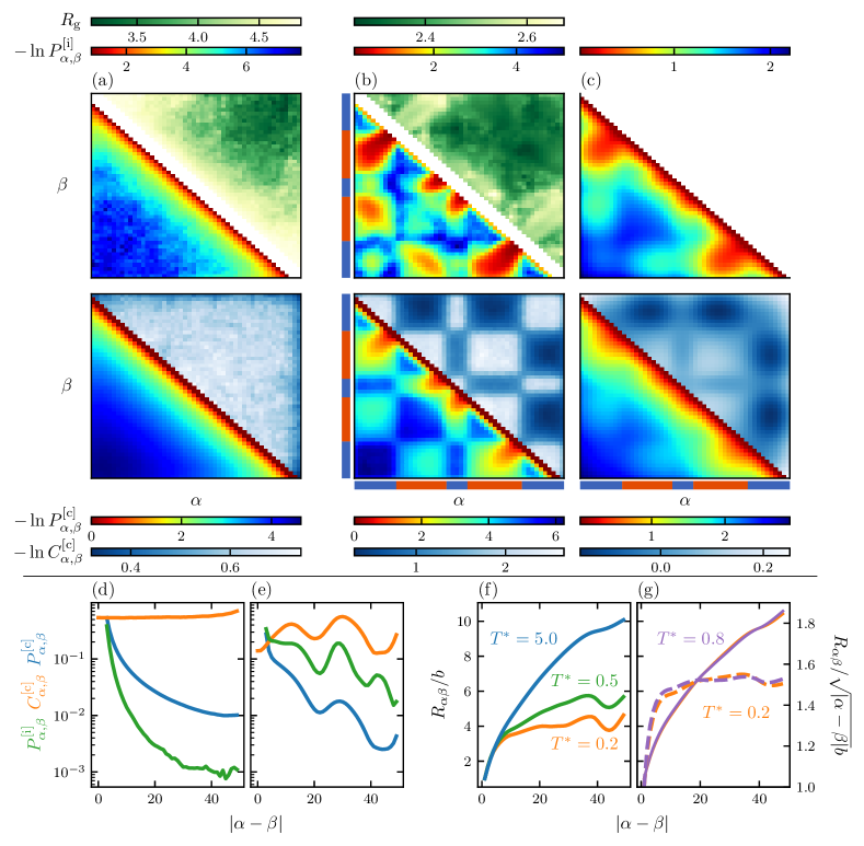
The origin of the performances of SCD and for is
explored by first considering how is related to
intrachain contacts for a homopolymer with favorable short-spatial-range
interactions (model described in Supporting Information).
In this baseline model, s conditioned upon
pairwise
contacts (Fig. 3a, top map, upper triangle) indicate
that more nonlocal (higher-order) contacts lead to
smaller . Sequence-local and nonlocal
interactions thus have different implications for . This basic
observation offers a semi-quantitative rationalization for SCD’s
better performance with regard to because,
as entailed by the original approximate analytical theory,kings2015
nonlocal electrostatic interactions (larger )
are more heavily
weighted in SCD than local interactions (smaller ).
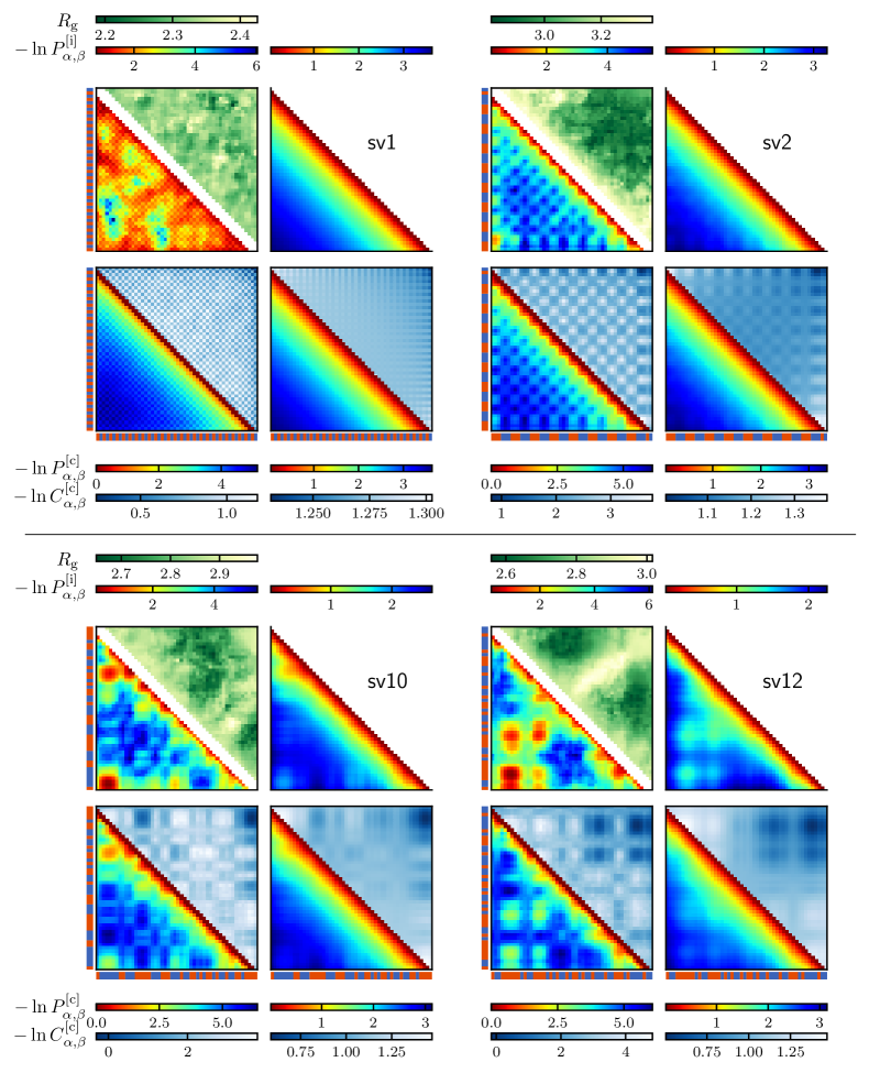
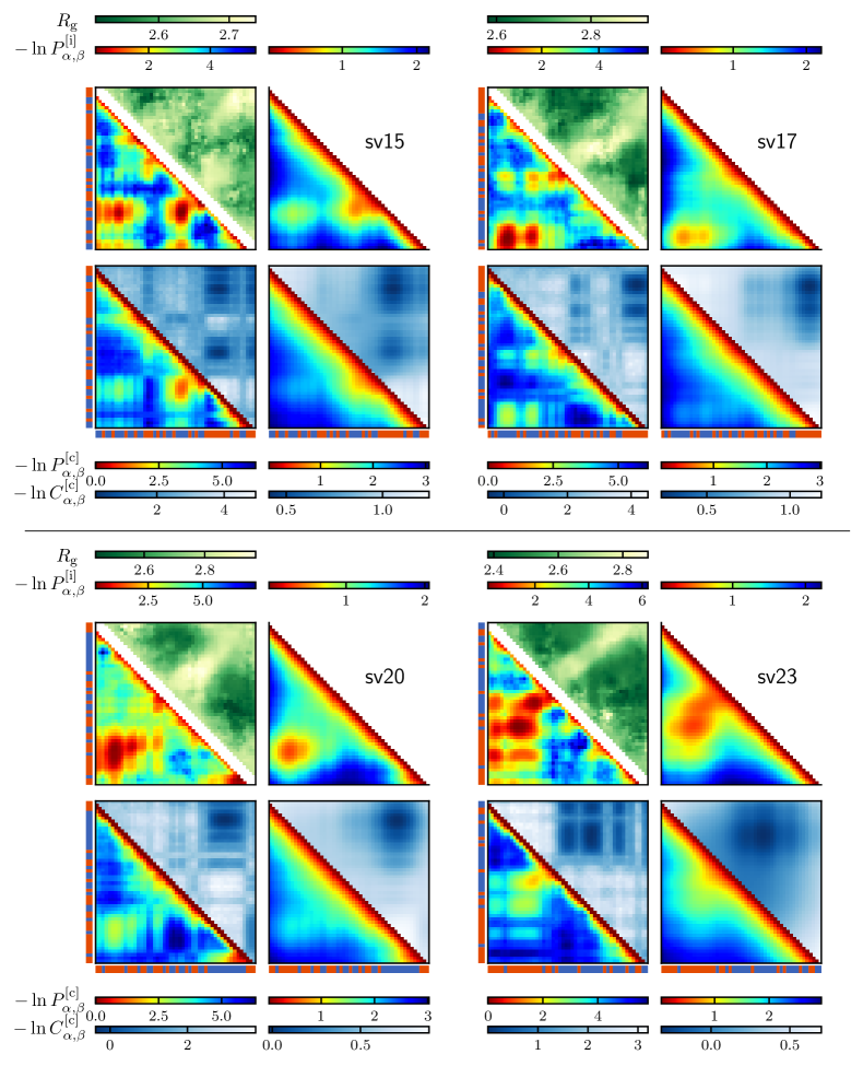
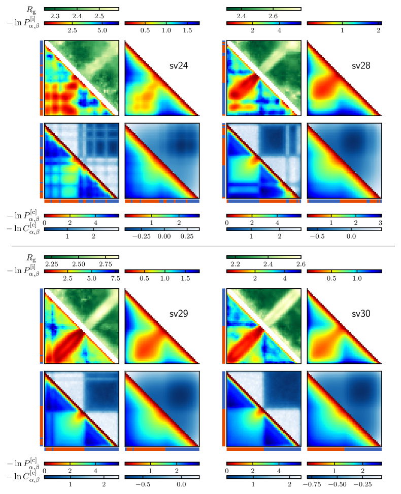
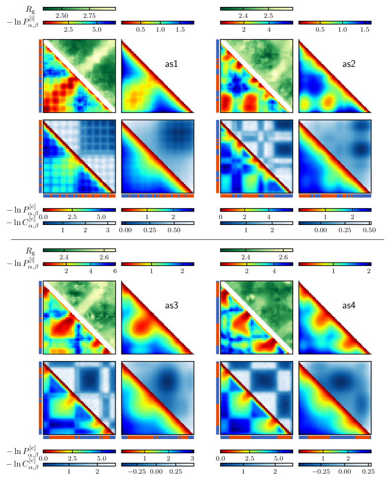
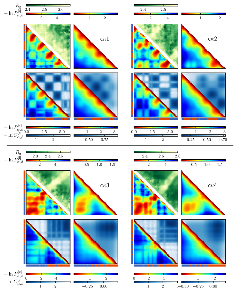
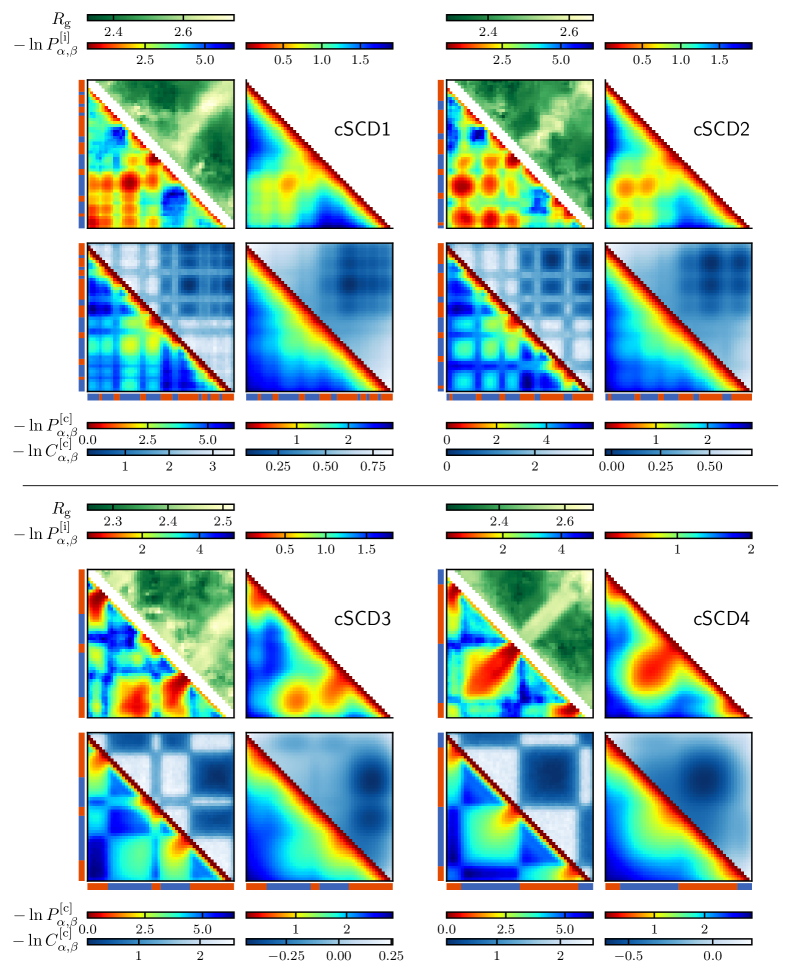
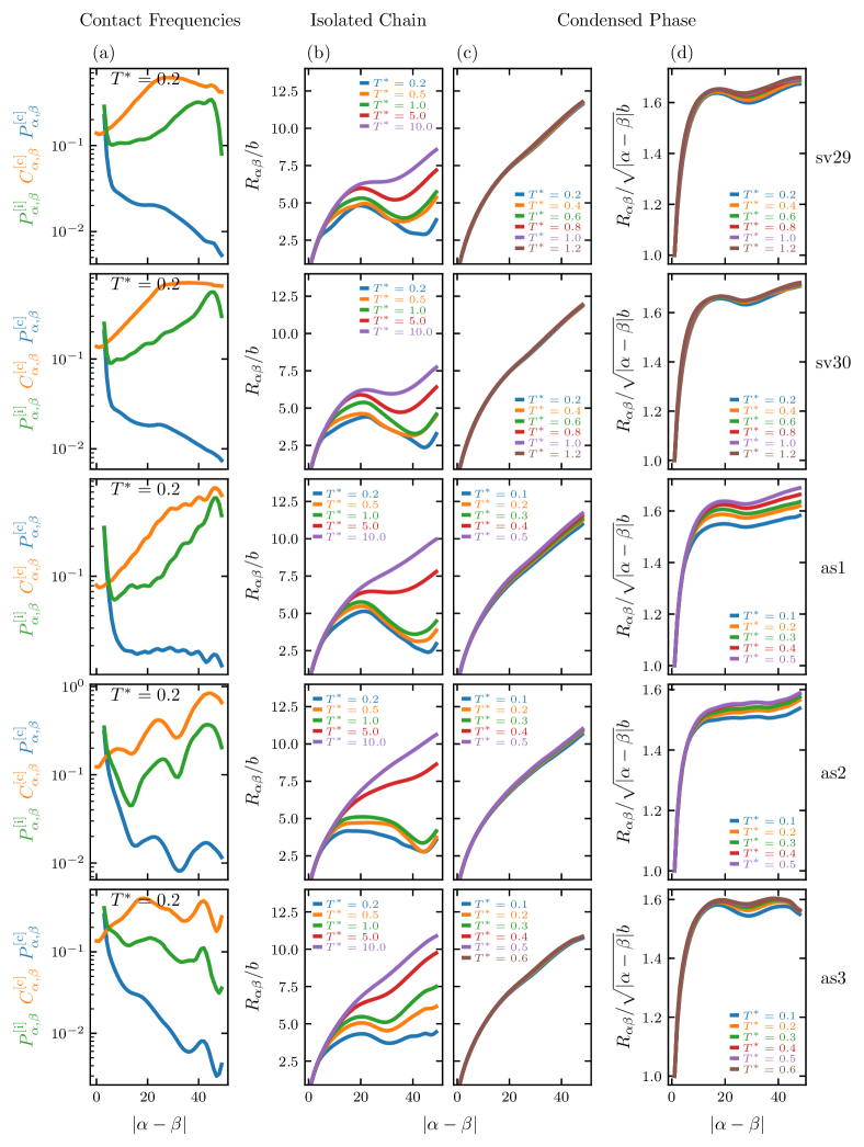
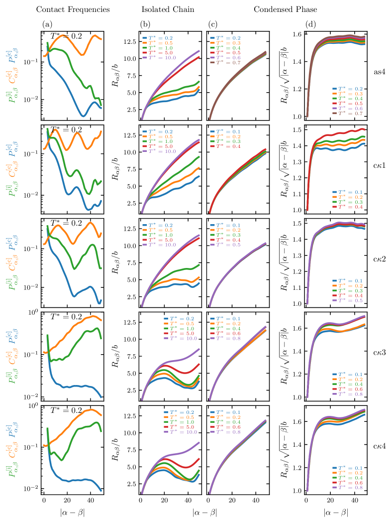
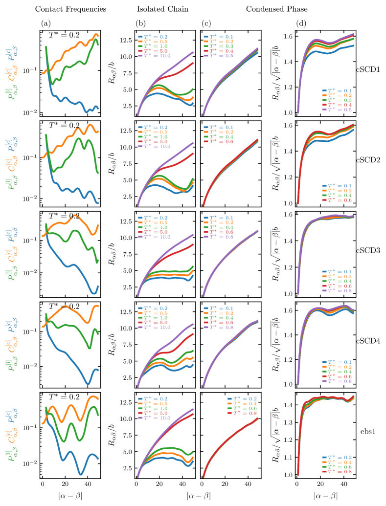
Additional information is provided by contact patterns (Fig. 3a–d).
The intrachain contact frequencies and
are the average numbers of
contacts between the th and th beads, respectively, of an
isolated chain (at infinite dilution) and a chain in the condensed phase,
whereas the interchain is the average number
of contacts between the th bead of one chain and the th
bead of another chain.
By definition,
,
, and
.
For the baseline homopolymer,
the isolated-chain ’s
pattern is typical of Gaussian or self avoiding walk
conformations, with substantially lower frequencies for higher order
contactsChanDill1990 (Fig. 3a, top map, lower triangle).
The condensed-phase intrachain pattern
(Fig. 3a, bottom map, lower triangle) shares a similar trend but
with less variation in contact frequency
(cf. heat map scales
for
and in Fig. 3a).
In contrast, the interchain
is quite insensitive to
except it is slightly higher when either , , or both,
are at or near the chain ends (Fig. 3a, bottom map, upper triangle).
Polyampholyte contact data are illustrated here by an example sequence.
The MD (Fig. 3b) and FTS (Fig. 3c) patterns are quite well
correlated, their differences likely arise from the differing
treatments of excluded volume in the two approaches.joanJPCL2019 ; Pal2021
Data for the other 25
sequences in Fig. 1b are in Fig. S4 of Supporting Information.
In Fig. 3b, the map exhibits sequence-specific
features as well as a contact-order dependence (top map, upper triangle)
indicating differential sequence-local versus nonlocal
effects on . Similar to the homopolymer (Fig. 3a),
the intrachain pattern of an isolated polyampholyte
(Fig. 3b,c top map, lower triangle) is similar to that of a polyampholyte
in the condensed phase (Fig. 3b,c bottom map, lower triangle).
Unlike the homopolymer, the isolated-chain intrachain
pattern (Fig. 3b,c top map, lower triangle) is similar also to the
condensed-phase interchain pattern (Fig. 3b,c bottom map, upper triangle).
This feature, which is echoed by the comparison in Fig. 3e below, applies to
the other 25 sequences as well.
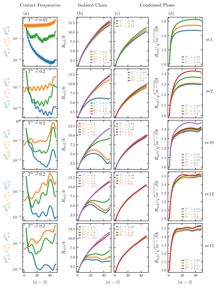
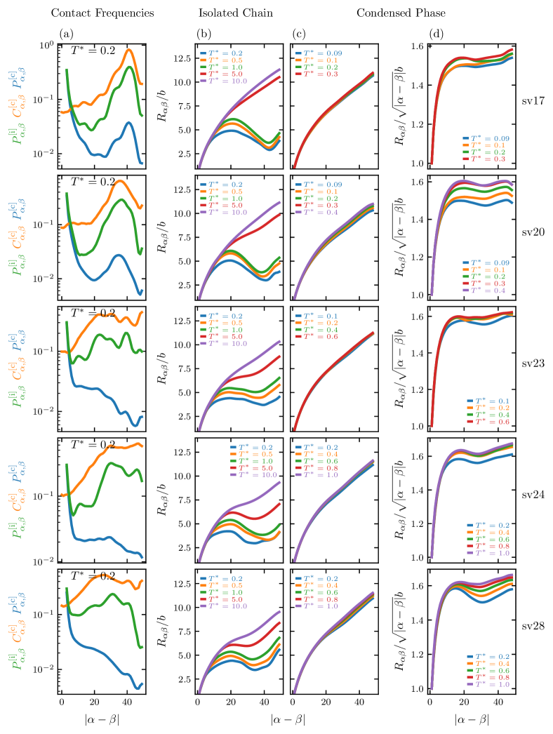
Averages of ,
, or
for a given are illustrated here using
the homopolymer model and the example sequence (Fig. 3d,e).
Similar salient features are exhibited by the other 25 sequences (Fig. S5 of
Supporting Information). Condensed-phase interchain
is least sensitive to
for the homopolymer (Fig. 3d) and for
polyampholytes (Fig. 3e). Notably,
the polyampholyte interchain (orange curve)
is closer to the isolated-chain intrachain
(green curve) than to the condensed-phase intrachain
(blue curve).
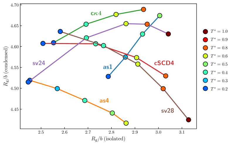
The root-mean-square distance between beads
and is highly sensitive to sequencerohit2013 and
temperature for an isolated polyampholyte
(Fig. 3f) as its decreases at low .
In contrast, Fig. 3g shows that depends only weakly
on . Depending on the sequence, can increase or decrease
slightly with (Fig. S6 of Supporting Information).
As in homopolymer melts,Flory1949 condensed-phase polyampholytes
adopt open, essentially Gaussian-like conformations
( constant except for
small in Fig. 3g), a
phenomenon also seen in recent simulations of biomolecular
condensates.MittalACS2023 ; PappuNatComm2023 ; Johnson2024 ; Mittal2024
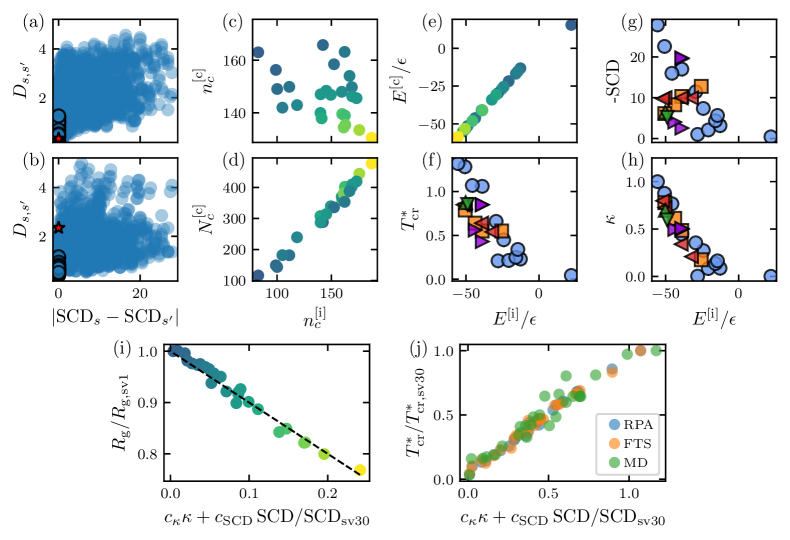
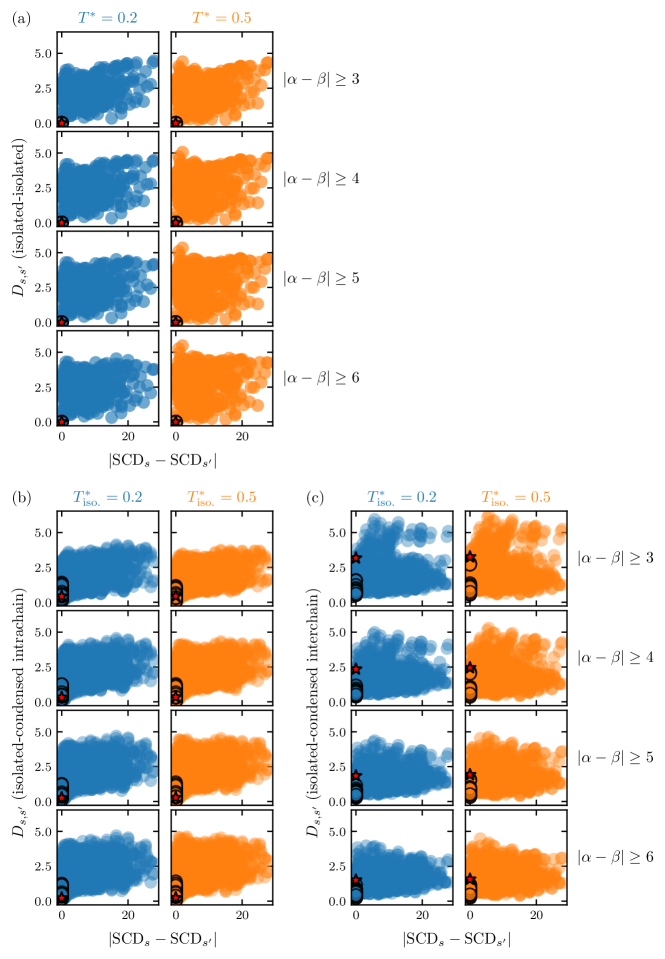
To gain further insights, we compare sequence-specific contact patterns such as those in Fig. 3b by the following symmetrized form of the Kullback-Leibler divergenceKL between contact frequencies and (contact maps) of a pair of sequences :
| (3) |
where serves to exclude local contacts—which are often
highly populated—from overwhelming the contact pattern’s quantitative
characterization,
and are normalized frequencies.
The comparisons of
with (Fig. 4a) and with
(Fig. 4b) entail significant scatter.
Nonetheless, the relatively low values for
(black circles) in Fig. 4b is consistent with the impression
from Fig. 3b,c that the patterns of isolated-chain intrachain
and condensed-phase interchain contacts are similar for a given polyampholyte.
This trend prevails for several other values
and another isolated-chain (Fig. S7 of Supporting Information),
underpinning correlations between sequence-dependent isolated-chain
and condensed-phase properties.
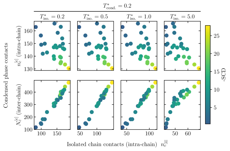
The relationship between isolated-chain and condensed-phase properties
is further elucidated by examining the total number of contacts made by
a polyampholyte. Whereas the number of intrachain contacts
of an isolated chain correlates poorly with that of a condensed-phase
chain (Fig. 4c) because of their significantly
different s (see above), an excellent correlation is seen
between the number of intrachain contacts of an isolated chain with
the number of interchain contacts in the condensed phase (Fig. 4d),
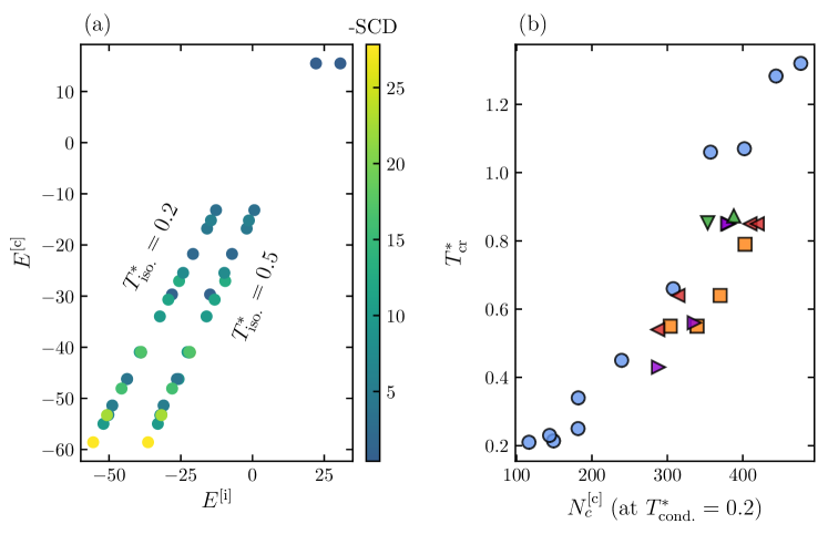
echoed by the excellent correlation between isolated-chain
and condensed-phase potential energies (Fig. 4e).
Similar trends are seen for other values of
(Fig. S8 and Fig. S9a of Supporting Information).
anticorrelates reasonably well with isolated-chain potential
energy (Fig. 4f), which expectedly correlates with
the number of interchain contacts (Fig. S9b in Supporting Information).
Notably, , in turn, anticorrelates quite well with
(Fig. 4h) but not so well with SCD (Fig. 4g), indicating that in some
situations can be a better predictor of LLPS propensity, suggesting
that differential effects of sequence-local versus nonlocal interactions
may be less prominent for LLPS than for isolated-chain .
This understanding is underscored by the fitting coefficients
for and for SCD in Fig. 4i,j
indicating that variation in
can be accounted for essentially entirely by SCD
()
but variation in is rationalized approximately equally
by and SCD ().
is not a good general predictor for though
correlates well with because
is not determined solely by .
For instance, two chains each constrained by one contact with
the same energy but different contact orders
can have very different s.
To recapitulate, many IDPs can exist in dilute and condensed phases serving
different biological functions. Single-chain IDP s in dilute
solutions, readily accessible experimentally,SongSAXS2021
have been used to benchmark MD potentials for
sequence-dependent IDP properties.KrestenNat2024 ; Alex2024
Isolated-chain contact maps,Zheng2023 related topological
constructs such as SCDMHuihuiKingsBJ2020 and energy
maps,Devarajan2022 and their relations with condensed-phase
interchain contact mapsKresten2021 ; bauer2022 have proven useful
in recent computational analyses.
For instance, isolated-chain intrachain and condensed-phase
interchain contacts are similar for heterochromatin protein 1
paralogsPhan2023 and EWS sequencesJohnson2024 but not
the TDP-43 C-terminal domain.mohanty2023
Here, our findings indicate a fundamental divergence in the differential
impact of local versus nonlocal sequence patterns on isolated,
single-chain and condensed-phase multiple-chain properties.
The differential impact is prominent for isolated-chain conformational
dimensions due to chain connectivity.ChanDill1990
It is substantially less
for LLPS propensity because
the multiple-chain nature of condensed-phase interactions
dampens—though not entirely abolish—the effects of contour separations
between residues along a single connected sequence due to the immense
number of configurations in which residues from different chains may interact.
This is a fundamental factor in the dilute/condensed-phase relationship
of IDPs that needs to be taken into account when devising improved
sequence pattern parameters for the characterization of physical
and functional IDP molecular features.Sabari2023 ; Moses2021
Inasmuch as such parameters’ aim is instant estimation of LLPS
propensity, theoretical quantities
that can be numerically computed efficiently—such as the
predicted by RPA-related theoriesWessenDasPalChan2022 —may just
serve the purpose practically even if they are not closed-form
mathematical expressions.
Supporting Information
Methodological and formulational details, supporting table, and
supporting figures
Acknowledgements. This work was supported by Canadian Institutes of Health Research (CIHR) grant NJT-155930 and Natural Sciences and Engineering Research Council of Canada (NSERC) grant RGPIN-2018-04351 to H.S.C. We are grateful for the computational resources provided generously by the Digital Research Alliance of Canada.
Figures (Main Text)
July 4, 2024
Supporting Information
for
Differential Effects of Sequence-Local versus Nonlocal
Charge Patterns on Phase Separation and
Conformational Dimensions of Polyampholytes as
Model Intrinsically Disordered Proteins
Tanmoy PAL,1,† Jonas WESSÉN,1,† Suman DAS,1,2,† and Hue Sun CHAN1,∗
1Department of Biochemistry, University of Toronto, Toronto, Ontario M5S 1A8, Canada
2Department of Chemistry, Gandhi Institute of Technology and Management, Visakhapatnam, Andhra Pradesh 530045, India
†Contributed equally.
∗Correspondence information:
Hue Sun CHAN.
E-mail: huesun.chan@utoronto.ca
Tel: (416)978-2697; Fax: (416)978-8548
Department of Biochemistry, University of Toronto,
Medical Sciences Building – 5th Fl.,
1 King’s College Circle, Toronto, Ontario M5S 1A8, Canada.
Methodological and Formulational Details
Estimating the sequence-space distribution
As outlined in the maintext, we investigate the relationship between the and parameters and its ramifications on isolated-chain and condensed-phase conformational properties by first calculating their distribution for electrically overall neutral 50mer polyampholytes (sequences with 50 beads). Following convention in an earlier work that used lysine (K) for the positively charged () and glutamic acid (E) for the negatively charged () monomers/residues along the chain sequence,rohit2013 we refer to the sequences under consideration as K/E sequence in the following discussion, keeping in mind, however, that K and E here refer only to and polymer beads with no sidechain structure, as in several previous simplified models.kings2015 ; lin2017 ; joanJPCL2019 ; suman2 Values for are computed in the present work using the expression defined in ref. (37).
The distribution is defined in such a way that is the number of possible sequences with values in a small region (two-dimensional bin) in the vicinity of . We compute using the Wang-Landau (WL) algorithm,WangLandau2001 which is a highly efficient flat-histogram method for estimating multi-peaked densities of states. However, before setting up the WL algorithm, prior knowledge about the the mathematically possible combinations is required since the WL algorithm relies on checking that all bins are evenly sampled.
To find the region in the -plane that can support 50mer K/E sequences, we utilize a genetic algorithm (GA) that is capable of scanning the space of sequences efficiently. Specifically, this GA takes an input target point in sequence space and attempts to generate a new sequence (, where the chain length ) with that maximizes the fitness function
| (S1) |
For a given target , the algorithm proceeds as follows:
-
1.
Generate an initial “population” of random electrically neutral K/E sequences (each with 25 K and 25 E).
-
2.
Each sequence in the population is used to generate “offspring” sequences. Every offspring sequence is generated from its parent sequence using one of the following prescriptions:
-
•
Single flip (50%): A randomly selected pair of K/E residues are interchanged.
-
•
Cluster move (45%): A randomly selected block of same-charge residues is moved one step (either left or right chosen at random), e.g., …EEEEEKKKK… …KEEEEEKKK… . As such, this is a special case of single flip. It serves to enhance sampling of blocky sequences.
-
•
New sequence (5%): An entirely new electrically neutral sequence with no relation to the parent sequence is randomly generated.
The three prescriptions are chosen at random with probabilities provided in parentheses above. We do not use crossover to generate offspring sequences (i.e. where multiple parent sequences are combined to generate offspring) as initial exploratory runs did not reveal any major advantage when using crossover.
-
•
-
3.
We next select out the offspring sequences using a diversity enhanced survivor selection algorithm. First, we evaluate the fitness of each offspring sequence , with , according to Eq. (S1), and select the sequence corresponding to the highest (least negative) as the first survivor. The fitness of the remaining sequences are then modified as where . This step punishes sequences that are identical or near-identical to the first selected survivor. The next survivor is then selected based on the updated fitnesses and the remaining sequences acquires new punishments depending on their similarity with . This procedure is repeated until have been selected.
-
4.
The survivors now constitute the population of the next generation and steps 2–3 are iterated until either a sequence with has been found or the 10th generation of iterations is reached.
The diversity enhanced survivor selection procedure prevents the algorithm from being trapped in the vicinity of a local fitness maximum since sequences are selected both according to having a high fitness and being dissimilar to other sequences with high fitness. The method was introduced to scan for experimentally viable parameter regions in extensions of the Standard Model in particle physics,CamargoMolinaMandal2018 but the survivor selection procedure was not outlined in full detail in ref. (38).
We coarse-grain the -plane into bins that cover the rectangular region (i.e., ), , where is the SCD value of the diblock sequence sv30 in ref. (13). The bin spanning the area and is indexed by (with ). The GA is first run for targets on the sites of an evenly spaced grid (marked by white dots in the left panel of Fig. S1a). Every new bin visited during the scan is recorded and the associated sequence is stored. With the exception of the first target iteration, the above step 1 of the GA is modified such that the initial population is generated as offspring of the previously stored sequence with nearest and to the target values instead of being randomly generated. The initial grid scan gives a rough estimate of region populated by sequences. Next, we iteratively run the GA for unvisited target bins adjacent to previously visited bins to map out the boundary of the region. Fig. S1a shows in the left panel the result of the GA scan, where bins for which a sequence was found are shown in black. White bins indicate target bins for which no sequence was found by the GA. For a few target bins, the GA was not able to find a sequence but the subsequent WL scan (described below) revealed sequences populating these bins. These mislabelled bins are shown in red in in the left panel of Fig. S1a.
The goal of the WL algorithm is to calculate the quantity representing the number of sequences with and in bin . To avoid numerical errors associated with large numbers, we (as is customary) formulate the algorithm in terms of rather than . Another central quantity in the WL algorithm is the histogram over the number of visits in bin . The WL algorithm operates as follows:
-
1.
Initialize for all and set the update factor .
-
2.
Generate random electrically neutral 50mer K/E sequences, , , , and compute their associated and values.
-
3.
Perform the updates
(S2) for the bin associated with each sequence.
-
4.
Check if is sufficiently flat. In this work, is deemed flat if
(S3) where the averages are taken only over bins known to be populated by sequences. If the flatness condition is satisfied we reset for all and update as .
-
5.
Propose an update for every sequence . The updates and their associated probabilities used in this work are
-
•
Single flip (80%): Flip the charges of a randomly selected pair of oppositely charged residues.
-
•
Multiple flips (20%): Perform single flips, where is a uniformly distributed random integer between 2 and 10.
Compute and for all proposed sequences and accept the updates with probabilities
(S4) where and refer to the bins associated with and , respectively. If a combination is encountered for which the associated bin was estimated by the GA as empty, the bin is re-labelled as non-empty and kept in all subsequent WL iterations.
-
•
-
6.
Repeat steps 3–5 until 25 WL “levels” have been completed, i.e., until is flat with .
-
7.
Re-weight where is the value of for the bin associated with the di-block sequence sv30. This step accounts for the double counting associated with reversed sequences but relies on the discretization being sufficiently fine such that only received contributions from sv30 and its reverse.
Our version of the WL algorithm differs from more standard implementationsIrback2013 ; IrbackWessen2015 since instantiations, rather than , of the system are evolved while modifying the same and . As such, our setup shares characteristics with the replica-exchange Wang-Landau method,Vogel2013 although we do not e.g., constrain the individual sequences to subregions of the -plane. We observe a dramatic decrease in computation time when and expect that the implementation can be made even more efficient by parallel computing since the sequence updates in Step 5 can be made independently in-between the and updates (see, e.g., refs. (87; 88; 89) for more sophisticated parallel WL algorithm implementations). The sought-after distribution, up to discretization errors, is now shown in the right panel of Fig. S1a as well as maintext Fig. 1a.
Given this , the moderate degree to which and are correlated may be quantified by the Pearson correlation coefficient
| (S5) |
where here denotes average over the
GA/WL-sampled distribution (thus the value between
SCD and is ).
The 26 overall-neutral polyampholyte sequences studied in this work
are given in maintext Fig. 1b and in Table S1, their
and values are listed in Fig. S1 and plotted on the
SCD versus plane in maintext Fig. 1a.
Field-theoretic formulation of polyampholyte conformations and phase separation
We study these model polyampholyte chain sequences using a field-theoretic formulation—using field-theoretic simulation (FTS) and random phase approximation (RPA)—as well as coarse-grained molecular dynamics (MD). As in our previous works (reviewed in ref. (68)), the present field-theoretic formulation is based on a Hamiltonian that accounts for chain connectivity, short-spatial-range excluded-volume repulsion and long-spatial-range electrostatic interactions for a system of polymers (polyampholyte chains) each consisting of monomer (beads). is given by
| (S6) |
where ( is the Boltzmann constant and is absolute temperature), is the reference root-mean-square bond length between two adjacent monomers along the chain sequence when non-bonded interactions are absent, is the position vector of the th bead of the th chain, is bead number density (matter density), is charge density, is the excluded volume parameter and is the Bjerrum length that we use to quantify electrostatic interaction strength, with denoting the protonic charge, and are vacuum and relative permittivities, respectively; and temperature in our field-theoretical models is quantified by the reduced temperature . An electric charge is associated with the th bead of each chain. In this work, we consider only overall charge neutral polyampholyte sequences, thus . To avoid potential singularities arising from modeling polymer beads as point particles, we model each bead as a normalized Gaussian distribution given by where (refs. (90; 67)). Accordingly, the bead number density and charge density are given, respectively, by
| (S7) | ||||
The field-theoretic model system defined by Eqs. S6
and S7 is analyzed using random phase approximation (RPA)
and field-theoretic simulation (FTS).
Random phase approximation (RPA).
An approximate analytical theory, termed RPA, can be derived from the
partition function formulated by path integrals based upon the
Hamiltonian in Eq. S6.
In the present study, all RPA calculations are performed within
the context of an implicit solvent polymer field theoryPal2021
(no explicit
solvent, unlike, e.g., in ref. (29)) with contact-excluded
volume interactions and unscreened Coulomb electrostatic interactions as
specified by Eq. S6 and, as mentioned,
UV (short-distance)-divergences are regulated
by Gaussian-smeared beads involving the function
as described above. In the present RPA calculations, we use a fixed
excluded volume parameter and a Gaussian smearing length
of .
The detailed mathematical formulation and the
computer code employed for our RPA calculations are documented and
available through our recent review.MiMB2023
Examples of phase diagrams computed using FTS and RPA for
the 26 polyampholyte sequences we study (maintext Fig. 1b, Fig. S1b, Table S1)
are provided in maintext Fig. 1d. A complete list of these phase
diagrams are documented in Fig. S2. The critical temperatures of these
sequences’ phase transitions in RPA and FTS are tabulated in Fig. S1b, whereas
the necessary details of our FTS methodology are provided below.
Radius of gyration and contact maps of chain conformations in the field-theoretic formulation. As a novel extension of our previous field-theoretic formulation, we now connect the radius of gyration () of a single polymer chain to the polymer beads’ pair-correlation functionPal2021 as follows:
| (S8) | ||||
where the bead center density is defined here by and denotes thermal averaging. Since the pair-correlation function depends only on the relative distance, we may perform a coordinate transformation such that and , with the associated Jacobian’s determinant , and thus rewrite Eq. (S8) as
| (S9) | ||||
where is the volume of the system. Because we have elected to use smeared Gaussian packets instead of point particles in our field-theoretic formulation to regularize short-range divergences as noted above, we will approximate the -function defined pair-correlation function defined above by smeared densities instead. Accordingly, in the formulation below for calculating of , we replace in Eq. (S8) by where as in Eq. (S7). Mathematically, (where ) is expected to be different from only in these functions’ variations over short distances . Since is integrated and weighted by in Eq. S9 for , the replacement of by is not numerically significant for the accuracy of the computed value of . For our purpose, however, the smearing that replace by is important as it allows and thus to be computed approximately using FTS.
By construction, Eq. S9 is applicable only for a single chain and needs to be extended for a multi-chain system. To do so, consider identical chains in a polyampholyte solution. We now choose one chain at random and recognize it as “tagged”. We denote the rest of the chains as “rest”. The total bead density can now be rewritten as where the superscripts “(t)” and “(r)” refer to “tagged” and “rest”, respectively. With this setup, we can now substitute the smeared self-correlation function of the tagged chain for in Eq. S9 to find the tagged chain’s in the multi-chain system, and can simply set in this general formulation to recover the formula for the of a single isolated chain. For clarity, we will denote this latter isolated-chain smeared self-correlation function by .
Correlation functions can also be utilized to compute residue-residue (bead-bead, or monomer-monomer) contact maps. To do so we only have to identify the monomers’ sequence positions along the polymer chains by rewriting the total bead center density for a multi-chain system as , where is sequence-position-specific density of the center of the th bead in the “tagged” chain/“rest” chains. As specified above for Eq. S8, unlike the smeared defined above, the bead center density (with subscript “c”) is defined by -function of position without smearing. We use unsmeared bead center densities for the computation of contacts because contacts are defined by spatial separations between bead centers. Now, the corresponding bead-specific unsmeared correlation functions can be defined as where . With this definition, we can compute the average contact frequency between the and monomers (beads) by spatially integrating the corresponding from radial distance up to a suitably chosen cutoff in for defining a contact, with the and cases accounting, respectively, for intrachain and interchain contacts. For the present work, we adopt the definitions
| (S10a) | ||||
| (S10b) | ||||
as intrachain (Eq. S10a) and
interchain (Eq. S10b)
contact frequencies, wherein
a radial cutoff distance of is used
for defining a bead-bead spatial contact.
Key steps in the field-theoretic simulation (FTS). Using the expression for the Hamiltonian in Eq. S6, the canonical partition function of our system of interest is given by
| (S11) |
Following standard procedures,FredricksonGanesanDrolet2002 ; Fredrickson2006 ; Pal2021 ; MiMB2023 ; WessenDasPalChan2022 we derive a field theory described by a field Hamiltonian (different from ) such that the partition function itself remains same as Eq. S11 up to an inconsequential overall multiplicative constant, viz.,
| (S12) |
in which two fluctuating auxiliary fields and are introduced, with
| (S13) |
where , , with “” denoting this spatial convolution henceforth. In Eq. S13, the single-chain partition function is given by
| (S14) |
where is the imaginery unit and
| (S15) |
Based on this particle-to-field reformulation, the equilibrium properties of the system can now be studied through the dynamics of the fields. Since the field Hamiltonian involves complex variables, we adoptFredrickson2006 a “Complex Langevin” (CL) prescriptionParisi1983 ; Klauder1983 inspired by stochastic quantizationParisiWu1981 ; ChanHalpern1986 for computing averages for the system defined by Eq. S13 by introducing dependence on a fictitious time to the fields, which then evolve dynamically in accordance to the Langevin equations
| (S16) | ||||
where is a fictitious time, and are fields of real-valued random numbers drawn from a normal distribution of zero mean and standard deviation that is nonzero only when and [, specifically, ]. This is the basic Langevin formulation of FTS. In Eq. S16, and are field operators for total bead density and charge density, respectively, which may be expressed as
| (S17) | ||||
where the forward () and backward () chain propagators and are constructed iteratively:
| (S18) | ||||
with and .
In practice, the differential field evolution equations Eqs. S16 have to be numerically solved in discretized space and discretized CL time. For the present work, every FTS is conducted in a cubic grid with a side length and we set following previous works. A CL time step and a semi-implicit CL time integration schemesii are employed. To compute the thermal average of any thermodynamic observable by FTS, the particle-based thermal average has to be replaced by an average over the field configurations of the corresponding field operator. The field operators could be derived by introducing appropriate “source” terms (fields) in the particle picture Hamiltonian (“” fields, see below), as is commonly practiced in theoretical particle physics.IZ If an observable has a field operator , then in practice the equilibrium field average of that specific operator is evaluated as an asymptotic CL time average through
| (S19) |
where is the maximum number of field configurations considered
(configurations are labeled by in the above equation
for selected values of fictitious time ) and
denotes field averaging.
The configurations at s and the total number of configurations
used in the averaging are chosen such that
the real part of the field averaged quantity has a reasonably small fluctuation over independent simulation runs and
the corresponding imaginary part is approximately zero. For all the FTS
computation, we set the excluded volume parameter .
Further details of our approach can be found in ref. (68).
FTS operators for correlation functions in the computation of polymer radius of gyration. As outlined above in the discussion preceding Eq. S10, to compute equilibrium properties of individual polymer chains in a multiple-chain system, we consider one chain, chosen at random, as tagged. The total bead density in Eq. S7 can then be rewritten as
| (S20) |
where the superscripts “(t)” and “(r)” denote ‘tagged’ and ‘rest’, respectively, with for the tagged chain and for the rest of the chains (untagged chains) given by
| (S21) | ||||
Field operators for total bead densities of “tagged” and “rest” chains are identified by introducing the source terms and in the original particle-picture Hamiltonian in Eq. S6 in the following manner:
| (S22) |
The resulting source-dependent partition function is now given by
| (S23) |
From this last expression (Eq. S23), we obtain the formal relations
| (S24) | ||||
where denotes thermal averaging. In the corresponding field theory representation, we have
| (S25) |
where
| (S26) | ||||
In this equation (Eq. S26), has the same functional form as that in Eq. S14. We can now apply the definitions Eq. S24 to Eq. S25 to arrive at and where
| (S27) | ||||
and is defined in Eq. S17 and, again, represents average over field configurations.
We can also compute the self-correlation function of the tagged chain from the partition function in Eq. S23 through the formal relation
| (S28) |
Applying this relation (Eq. S28) to Eq. S23 results in
| (S29) |
where, following ref. (30), we have avoided computing a functional double derivative of .
When there is only a single isolated chain in the system, the self-correlation function is obtained by setting and in the above derivation, yielding
| (S30) |
Utilizing translational invariance of our systems, we can write
| (S31) | ||||
where, when the density smearing described above is applied, is the Fourier transform of the smeared density . In that case, it follows that where is the Fourier transform of the smearing function and is the Fourier transform of the bead center density . This implies that when Gaussian smearing is utilized in our formulation, the bead center-bead center pair correlation function [] can now be expressed as
| (S32) |
FTS operators for correlation functions in the computation of contact maps of polymers. As noted above, the starting point for contact map computations is the (unsmeared) bead center density correlation functions. As noted above in the discussion preceding Eq. S10, we first rewrite the total bead center density as
| (S33) |
where and could be expressed in terms of the bead-position-specific densities along the chains through
| (S34) | ||||
We now introduce monomer (residue)-specific source terms in the interaction Hamiltonian Eq. S6:
| (S35) |
The corresponding partition function is
| (S36) |
From this expression (Eq. S36), the average density of the th bead center is formally
| (S37) |
and the correlation function between any two bead center is given by
| (S38) |
where . The corresponding partition function in the field picture is then given by
| (S39) |
where
| (S40) | ||||
and the absence of breve in the source terms on the right hand side in the above equation means that the source terms are not smeared. In Eq. S40, has the same functional form as that in Eq. S14, which can be written explicitly as
| (S41) | ||||
where , and
| (S42) |
with defined by Eq. S15. Substituting Eq. S37 into Eq. S39 then results in and , with
| (S43) | ||||
As discussed above in conjunction with eq. S10b, the numbers of interchain contacts and thus interchain contact maps are determined in our formulation via the cross correlation function between the th bead center of the tagged chain and the th bead center of the rest of the chains. This cross correlation is readily obtained by taking double functional derivatives of the partition function in Eq. S39 in accordance with Eq. S38 to yield
| (S44) |
for the calculation of interchain numbers of contacts in Eq. S10b. Similarly, for the numbers of intrachain contacts and intrachain contact maps, we compute, in accordance with Eq. S10a, the correlations between the beads of the tagged chain as follows:
| (S45) | ||||
where
| (S46) | ||||
with . In the last Eq. S46, is a -dependent (Fourier-transformed) single chain restricted partition function, given by
| (S47) | ||||
This implies that in order to evaluate
in Eq. S46, we need to first evaluate
at each and then perform
an inverse Fourier transform according to the last equality in
Eq. S46. Therefore,
for a spatial lattice
used for FTS, ideally we should calculate the values of
on a (reciprocal) -space lattice
of the same size, i.e., determine
times for each pair for each field
configuration (Eq. S47).
This would be exceedingly computationally intensive.
For computational efficiency, we consider instead a slightly more
coarse-grained -space
lattice of dimensions
with , such that the resolution of its
reciprocal space, i.e., the original space, becomes
with .
Nonetheless, we still compute the
volume integrals
in Eq. (S47) in the original
spatial lattice with
resolution .
In this way, we reduce the computational cost by times.
Thus, for all the intrachain FTS contact maps presented here, ,
, and the final equilibrium field configurations of
independent runs are used for field averaging. As a check on the accuracy
of this coarse-graining, we have also computed contact maps with
reciprocal lattice and saw no visible difference from
the results.
Volume integration in simulation boxes with periodic boundary conditions. To perform volume integration of an isotropic function in a cubic box () with periodic boundary conditions, the integration measure has to be modified owing to the periodic boundary conditions, as follows:
| (S48) |
where
| (S49) |
such that integration of any isotropic function from to any upper integration limit on the periodic lattice is specified by
| (S50) |
Numerical estimation of in FTS Binodal phase boundaries in FTS are computed using the method described in ref. (68). In the present study, to estimate the critical temperature from the FTS binodals, we adopt—as in recent coarse-grained MD studies of biomolecular condensatessuman2 ; dignon18 —the scaling approach outlined in ref. (61), which assumes that low- and high-density phase concentrations, denoted by and , respectively, follow the relations
| (S51a) | ||||
| (S51b) | ||||
where , and , , critical density ,
and are free fitting parameters. Now, for
each sequence, we use the highest two simulated for fitting.
First, we estimate and by fitting the
numerical values of to
Eq. S51b.
Next, we apply this fitted to Eq. (S51a)
to fit the numerical values of
to yield fitted values for and .
These fitted parameters are then applied to obtain
and as functions of
from the two relations in
Eq. S51. In Fig. S2 (see below)
and maintext Fig. 1d, these fitted functions are used to construct
continuous curves through the fitted
critical point and the four simulated binodal
and
datapoints with the two highest , whereas
the numerical FTS and
datapoints for the dilute and dense branches of the binodals
for the rest of the simulated are simply connected by lines
as guides for the eye.
Coarse-grained molecular dynamics (MD) model of polyampholyte conformations and phase separation
The coarse-grained MD model here is essentially identical to the “hard-core repulsion” model we used previously in ref. (37) for the simulation of “sv”rohit2013 and “as”suman2 polyampholyte sequences. The only difference is that the repulsive part of the Lennard-Jones (LJ) potential is set to zero for in the present study—where is the reference (equilibrium) bond length between successive beads (monomers) along the chain sequence—instead of for in ref. (37). MD simulation in the present work is carried out using the protocol described in refs. (37; 48). A contact is defined to exist between two monomers when their center-of-mass spatial separation is within .
| Name | Sequence |
|---|---|
| sv1 | EKEKEKEKEKEKEKEKEKEKEKEKEKEKEKEKEKEKEKEKEKEKEKEKEK |
| sv2 | EEEKKKEEEKKKEEEKKKEEEKKKEEEKKKEEEKKKEEEKKKEEEKKKEK |
| sv10 | EKKKKKKEEKKKEEEEEKKKEEEKKKEKKEEKEKEEKEKKEKKEEKEEEE |
| sv12 | EKKEEEEEEKEKKEEEEKEKEKKEKEEKEKKEKKKEKKEEEKEKKKKEKK |
| sv15 | KKEKKEKKKEKKEKKEEEKEKEKKEKKKKEKEKKEEEEEEEEKEEKKEEE |
| sv17 | EKEKKKKKKEKEKKKKEKEKKEKKEKEEEKEEKEKEKKEEKKEEEEEEEE |
| sv20 | EEKEEEEEEKEEEKEEKKEEEKEKKEKKEKEEKKEKKKKKKKKKKKKEEE |
| sv23 | EEEEEKEEEEEEEEEEEKEEKEKKKKKKEKKKKKKKEKEKKKKEKKEEKK |
| sv24 | EEEEKEEEEEKEEEEEEEEEEEEKKKEEKKKKKEKKKKKKKEKKKKKKKK |
| sv28 | EKKKKKKKKKKKKKKKKKKKKKEEEEEEEEEEEEEEEEEEKKEEEEEKEK |
| sv29 | KEEEEKEEEEEEEEEEEEEEEEEEEEEKKKKKKKKKKKKKKKKKKKKKKK |
| sv30 | EEEEEEEEEEEEEEEEEEEEEEEEEKKKKKKKKKKKKKKKKKKKKKKKKK |
| as1 | KKKKKEKKKKKEKKKKEKKKKEKKEKEEEKEEEEKEEEEKEEEEKEEEEE |
| as2 | EEEEEEEEKKEKKKKEEEEEEEEEEEKKKKEEEKEKEKKKKKKKKKKKKK |
| as3 | KKKKEEEEEEEEEEEEEEEEEEKKEKKKKKKKKKKKKKKEKEEEEEKKKK |
| as4 | KKKKKKEEEEEEEEEEEEEEEKKKKKKKKKKKKKKKKKKEEEEEEEEEEK |
| c1 | KKKEEEEEEEEKKKKKKKKKKEEEEEEEEEEKKKKKKKKKEEKEEEKEKE |
| c2 | KKKEEEEEEEKKEEEEEKKKEKKKKKKKKEEEEEEEEEEEEKKKKKKKKK |
| c3 | KKKKKKKKKKKKKKKEKKKKKEKKEEEEKEEEEEKEEEEEKEEEEEEEEE |
| c4 | KKKKKKKKKKEKKKKKEKKKKEKKKKEEKEEEEEKEEEEEEEEEEEEEEE |
| cSCD1 | KKKKEKKKKEEKKKKKKKEEKKKKKEEEEKKEEEEEEEKEEKEEEKEEEE |
| cSCD2 | KEKKKKKKKKEEKKKKKKEEKKKKKEEEEEKKEEEEEEEEKKKEEEEEEE |
| cSCD3 | EEEEEEEKKKKKKKKKKKKKKKEEEKKKKKKKKKKEEEEEEEEEEEEEEE |
| cSCD4 | EEEEEKKKKKKKKKKKKKKKKKKKKEEEEEEEEEEEEEEEEEEEEKKKKK |
| obs1 | KKKKKKKKKKEEEEEEEEEEEEKKKKKEEEEEEEEEEEEEKKKKKKKKKK |
| ebs1 | EEEEEEEEEKKKKKKKKEEEEEEEEKKKKKKKKEEEEEEEEKKKKKKKKK |
Supporting Figures
References
References
- (1) Shin, Y.; Brangwynne, C. P. Liquid phase condensation in cell physiology and disease. Science 2017, 357, eaaf4382.
- (2) Lyon, A. S.; Peeples, W. B.; Rosen, M. K. A framework for understanding the functions of biomolecular condensates across scales. Nat. Rev. Mol. Cell Biol. 2021, 22, 215–235.
- (3) Pappu, R. V.; Cohen, S. R.; Dar, F.; Farag, M.; Kar, M. Phase transitions of associative biomacromolecules. Chem. Rev. 2023, 123, 8945–8987.
- (4) Shen, Z.; Jia, B.; Xu, Y.; Wessén, J.; Pal, T.; Chan, H. S.; Du, S.; Zhang, M. Biological condensates form percolated networks with molecular motion properties distinctly different from dilute solutions. eLife 2023 12, 81907.
- (5) Zhou, H.-X.; Kota, D.; Qin, S.; Prasad, R. Fundamental aspects of phase-separated biomolecular condensates. Chem. Rev. 2024, 124, 8550–8595.
- (6) Nott, T. J.; Petsalaki, E.; Farber, P.; Jervis, D.; Fussner, E.; Plochowietz, A.; Craggs, T. D.; Bazett-Jones, D. P.; Pawson, T.; Forman-Kay, J. D., et al. Phase transition of a disordered nuage protein generates environmentally responsive membraneless organelles. Mol. Cell 2015, 57, 936–947.
- (7) Lin, Y.-H.; Forman-Kay, J. D.; Chan, H. S. Sequence-specific polyampholyte phase separation in membraneless organelles. Phys. Rev. Lett. 2016, 117, 178101.
- (8) Bremer, A.; Farag, M.; Borcherds, W. M.; Peran, I.; Martin, E. W.; Pappu, R. V.; Mittag, T. Deciphering how naturally occurring sequence features impact the phase behaviours of disordered prion-like domains. Nat. Chem. 2022, 14, 196–207.
- (9) Vernon, R. M.; Chong, P. A.; Tsang, B.; Kim, T. H.; Bah, A.; Farber, P.; Lin, H.; Forman-Kay, J. D. Pi-Pi contacts are an overlooked protein feature relevant to phase separation. 2018, eLife 7, e31486.
- (10) Chen, T.; Song, J.; Chan, H. S. Theoretical perspectives on nonnative interactions and intrinsic disorder in protein folding and binding. Curr. Opin. Struct. Biol. 2015, 30, 32–42.
- (11) Bauer, D. J.; Stelzl, L. S.; Nikoubashman, A. Single-chain and condensed-state behavior of hnRNPA1 from molecular simulations. J. Chem. Phys. 2022 157, 154903.
- (12) Hazra, M. K.; Levy, Y. Cross-talk of cation- interactions with electrostatic and aromatic interactions: A salt-dependent trade-off in biomolecular condensates. J. Phys. Chem. Lett. 2023, 14, 8460–8469.
- (13) Das, R. K.; Pappu, R. V. Conformations of intrinsically disordered proteins are influenced by linear sequence distributions of oppositely charged residues. Proc. Natl. Acad. Sci. U.S.A. 2013, 110, 13392–13397.
- (14) Sawle, L.; Ghosh, K. A theoretical method to compute sequence dependent configurational properties in charged polymers and proteins. J. Chem. Phys. 2015, 143, 085101.
- (15) Welsh, T. J.; Krainer, G.; Espinosa, J. R.; Joseph, J. A.; Sridhar, A.; Jahnel, M.; Arter, W. E.; Saar, K. L.; Alberti, S.; Collepardo-Guevara, R.; Knowles, T. P. J. Surface electrostatics govern the emulsion stability of biomolecular condensates. Nano Lett. 2022, 22, 612–621.
- (16) Lyons, H.; Veettil, R. T.; Pradhan, P.; Fomero, C.; De La Cruz, N.; Ito, K.; Eppert, M.; Roeder, R. G.; Sabari, B. R. Functional partitioning of transcriptional regulators by patterned charge blocks. Cell 2023, 186, 327–345.
- (17) Flory, P. J.; Fox, T. G., Jr. Treatment of intrinsic viscosities. J. Am. Chem. Soc. 1951, 73, 1904–1908.
- (18) Shultz, A. R.; Flory, P. J. Phase equilibria in polymer-solvent systems. J. Am. Chem. Soc. 1952, 74, 4760–4767.
- (19) Qian, D.; Michaels, T. C. T.; Knowles, T. P. J. Analytical solution to the Flory-Huggins model. J. Phys. Chem. Lett. 2022, 13, 7853–7860.
- (20) Panagiotopoulos, A. Z.; Wong, V.; Floriano, M. A. Phase equilibtia of lattice polymers from histogram reweighting Monte Carlo simulations. Macromolecules 1998, 31, 912–918.
- (21) Wang, R.; Wang, Z.-G. Theory of polymer chains in poor solvent: Single-chain structure, solution thermodynamics, and point. Macromolecules 2014, 47, 4094–4102.
- (22) Lin, Y.-H.; Chan, H. S. Phase separation and single-chain compactness of charged disordered proteins are strongly correlated. Biophys, J. 2017, 112, 2043–2046.
- (23) Dignon, G. L.; Zheng, W.; Best, R. B.; Mittal, J. Relation between single-molecule properties and phase behavior of intrinsically disordered proteins. Proc. Natl. Acad. Sci. U.S.A. 2018, 115, 9929–9934.
- (24) Amin, A. N.; Lin, Y.-H.; Das, S.; Chan, H. S. Analytical theory for sequence-specific binary fuzzy complexes of charged intrinsically disordered proteins. J. Phys. Chem. B 2020, 124, 6709–6720.
- (25) Riback, J. A.; Katanski, C. D.; Kear-Scott, J. L.; Pilipenko, E. V.; Rojek, A. E.; Sosnick, T. R.; Drummond, D. A. Stress-triggered phase separation is an adaptive, evolutionarily tuned response. Cell 2017, 168, 1028–1040.
- (26) von Bülow, S.; Tesei, G.; Lindorff-Larsen, K. Prediction of phase separation propensities of disordered proteins from sequence. bioRiv – The Preprint Server for Biology, Cold Spring Harbor Laboratory, https://doi.org/10.1101/2024.06.03.597109 (accessed 2024-07-24).
- (27) McCarty, J.; Delaney, K. T.; Danielsen, S. P. O.; Fredrickson, G. H.; Shea, J.-E. Complete phase diagram for liquid-liquid phase separation of intrinsically disordered proteins. J. Phys. Chem. Lett. 2019, 10, 1644–1652.
- (28) Danielsen, S. P. O.; McCarty, J.; Shea, J.-E.; Delaney, K. T.; Fredrickson, G. H. Molecular design of self-coacervation phenomena in block polyampholytes. Proc. Natl. Acad. Sci. U.S.A. 2019, 116, 8224–8232.
- (29) Wessén, J., Pal, T., Das, S., Lin, Y.-H. & Chan, H. S. A simple explicit-solvent model of polyampholyte phase behaviors and its ramifications for dielectric effects in biomolecular condensates. J. Phys. Chem. B 2021 125, 4337–4358.
- (30) Pal, T.; Wessén, J.; Das, S.; Chan, H. S. Subcompartmentalization of polyampholyte species in organelle-like condensates is promoted by charge-pattern mismatch and strong excluded-volume interaction. Phys. Rev. E 2021, 103, 042406.
- (31) Dill, K. A. Dominant forces in protein folding. Biochemistry 1990, 29, 7133-7155.
- (32) Chan, H. S.; Dill, K. A. The effects of internal constraints on the configurations of chain molecules. J. Chem. Phys. 1990, 92, 3118–3135. Erratum: J. Chem. Phys. 1997, 107, 10353.
- (33) Dill, K. A.; Fiebig, K. M.; Chan, H. S. Cooperativity in protein folding kinetics. Proc. Natl. Acad. Sci. U.S.A. 1993, 90, 1942–1946.
- (34) Plaxco, K. W.; Simons, K. T.; Baker, D. Contact order, transition state placement and the refolding rates of single domain proteins. J. Mol. Biol. 1998, 277, 985–994.
- (35) Chan, H. S. Protein folding: Matching speed and locality. Nature 1998, 392, 761–763.
- (36) Chan, H. S.; Zhang, Z.; Wallin, S.; Liu, Z. Cooperativity, local-nonlocal coupling, and nonnative interactions: Principles of protein folding from coarse-grained models. Annu. Rev. Phys. Chem. 2011, 62, 301–326.
- (37) Das, S.; Amin, A. N.; Lin, Y.-H.; Chan, H. S. Coarse-grained residue-based models of disordered protein condensates: Utility and limitations of simple charge pattern parameters. Phys. Chem. Chem. Phys. 2018, 20, 28558–28574.
- (38) Camargo-Molina, J. E., Mandal, T., Pasechnik, R. & Wessén, J. Heavy charged scalars from fusion: a generic search strategy applied to a 3HDM with family symmetry. Journal of High Energy Physics (JHEP) 2018, 2018, 24.
- (39) Wang, F. & Landau, D. P. Efficient, multiple-range random walk algorithm to calculate the density of states. Phys. Rev. Lett. 2001, 86, 2050–2053.
- (40) Hazra, M. K.; Levy, Y. Charge pattern affects the structure and dynamics of polyampholyte condensates. Phys. Chem. Chem. Phys. 2020, 22, 19368–19375.
- (41) Devarajan, D. S.; Wang, J.; Szała-Mendyk, B.; Rekhi, S.; Nikoubashman, A.; Kim, Y. C.; Mittal, J. Sequence-dependent material properties of biomolecular condensates and their relation to dilute phase conformations. Nat. Comm. 2024, 15, 1912.
- (42) Rana, U.; Wingreen, N. S.; Brangwynne, C. P.; Panagiotopoulos, A. Z. Interfacial exchange dynamics of biomolecular condensates are highly sensitive to client interactions. J. Chem. Phys. 2024, 160, 145102.
- (43) Ruff, K. M. Predicting conformational properties of intrinsically disordered proteins from sequence. Methods Mol. Biol. 2021, 2141, 347–389.
- (44) Cohan, M. C.; Shinn, M. K.; Lalmansingh, J. M.; Pappu, R. V. Uncovering non-random binary patterns within sequences of intrinsically disordered proteins. J. Mol. Biol. 2022, 434, 167373.
- (45) Huihui, J.; Firman, T.; Ghosh, K. Modulating charge patterning and ionic strength as a strategy to induce conformational changes in intrinsically disordered proteins. J. Chem. Phys. 2018, 149, 085101.
- (46) Wang, J.; Choi, J. M.; Holehouse, A. S.; Lee, H. O.; Zhang, X.; Jahnel, M.; Maharana, S.; Lemaitre, R.; Pozniakovsky, A.; Drechsel, D., et al. A molecular grammar governing the driving forces for phase separation of prion-like RNA binding proteins. Cell 2018, 174, 688–699.
- (47) Zheng, W.; Dignon, G.; Brown, M.; Kim, Y. C.; Mittal, J. Hydropathy patterning complements charge patterning to describe conformational preferences of disordered proteins. J. Phys. Chem. Lett. 2020, 11, 3408–3415.
- (48) Wessén, J.; Das, S.; Pal, T.; Chan, H. S. Analytical formulation and field-theoretic simulation of sequence-specific phase separation of protein-like heteropolymers with short- and long-spatial-range interactions. J. Phys. Chem. B 2022, 126, 9222–9245. Correction: J. Phys. Chem. B 2023, 127, 11100.
- (49) Rekhi, S.; Devarajan, D. S.; Howard, M. P.; Kim, Y. C.; Nikoubashman, A.; Mittal, J. Role of strong localized vs. weak distributed interactions in disordered protein phase separation. J. Phys. Chem. B 2023, 127, 3829–3838.
- (50) Rekhi, S.; Garcia, C. C.; Barai, M.; Rizuan, A.; Schuster, B. S.; Kiick, K.; Mittal J. Expanding the molecular language of protein liquid-liquid phase separation. Nat. Chem. 2024, 16, 1113–1124.
- (51) Lin, Y.-H.; Brady, J. P.; Chan, H. S.; Ghosh, K. A unified analytical theory of heteropolymers for sequence-specific phase behaviors of polyelectrolytes and polyampholytes. J. Chem. Phys. 2020, 152, 045102.
- (52) Lin, Y.-H.; Kim, T. H.; Das, S.; Pal, T.; Wessén, J.; Rangadurai, A. K.; Kay, L. E.; Forman-Kay, J. D.; Chan, H. S. Electrostatics of salt-dependent reentrant phase behaviors highlights diverse roles of ATP in biomolecular condensates. arXiv – Quantitative Biology (q-bio), Biomolecules (Cornell University) https://arxiv.org/abs/2401.04873 (accessed 2024-07-24).
- (53) Mahdi, K. A.; Olvera de la Cruz, M. Phase diagrams of salt-free polyelectrolyte semidilute solutions. Macromolecules 2000, 33, 7649–7654.
- (54) Ermoshkin, A. V.; Olvera de la Cruz, M. A modified random phase approximation of polyelectrolyte solutions. Macromolecules 2003, 36, 7824–7832.
- (55) Cheong, D. W.; Panagiotopoulos, A. Z. Phase behaviour of polyampholyte chains from grand canonical Monte Carlo simulations. Mol. Phys. 2005, 103, 3031–3044.
- (56) Fredrickson, G. H. The Equilibrium Theory of Inhomogeneous Polymers. Oxford University Press, Oxford, U.K. (2006).
- (57) Sing, C. E.; Perry, S. L. Recent progress in the science of complex coacervation. Soft Matter 2020, 16, 2885–2914.
- (58) Jacobs, W. M. Theory and simulation of multiphase coexistence in biomolecular mixtures. J. Chem. Theory Comput. 2023, 19, 3429–3445.
- (59) Parisi, G. On complex probabilities. Phys. Lett. B 1983, 131, 393–395.
- (60) Klauder, J. R. A Langevin approach to fermion and quantum spin correlation functions. J. Phys. A: Math. Gen. 1983, 16, L317–L319.
- (61) Silmore, K. S.; Howard, M. P.; Panagiotopoulos, A. Z. Vapour–liquid phase equilibrium and surface tension of fully flexible lennard–jones chains. Mol. Phys. 2017, 115, 320–327.
- (62) Dignon, G. L.; Zheng, W.; Kim, Y. C.; Best, R. B.; Mittal, J. Sequence determinants of protein phase behavior from a coarse-grained model. PLoS Comput. Biol. 2018, 14, e1005941.
- (63) Das, S.; Lin, Y.-H.; Vernon, R. M.; Forman-Kay, J. D.; Chan, H. S. Comparative roles of charge, , and hydrophobic interactions in sequence-dependent phase separation of intrinsically disordered proteins. Proc. Natl. Acad. Sci. U.S.A. 2020, 117, 28795–28805.
- (64) Joseph, J. A.; Reinhardt, A.; Aguirre, A.; Chew, P. Y.; Russell, K. O.; Espinosa, J. R.; Garaizar, A.; Collepardo-Guevara, R. Physics-driven coarse-grained model for biomolecular phase separation with near-quantitative accuracy. Nat. Comput. Sci. 2021, 1, 732–743.
- (65) Tesei, G.; Schulze, T. K.; Crehuet, R.; Lindorff-Larsen, K. Accurate model of liquid-liquid phase behavior of intrinsically disordered proteins from optimization of single-chain properties. Proc. Natl. Acad. Sci. U.S.A. 2021, 118, e2111696118.
- (66) Fredrickson, G. H.; Ganesan, V.; Drolet, F. Field-theoretic computer simulation methods for polymers and complex fluids. Macromolecules 2022, 35, 16–39.
- (67) Riggleman, R. A., Kumar, R. & Fredrickson, G. H. Investigation of the interfacial tension of complex coacervates using field-theoretic simulations. J. Chem. Phys. 2012, 136, 024903.
- (68) Lin, Y.-H.; Wessén, J.; Pal, T.; Das, S.; Chan, H.S. Numerical techniques for applications of analytical theories to sequence-dependent phase separations of intrinsically disordered proteins. Methods Mol. Biol. 2023, 2563, 51–94.
- (69) Flory, P. J. The configuration of real polymer chains. J. Chem. Phys. 1949, 17, 303–310.
- (70) Wang, J.; Devarajan, D. S.; Nikoubashman, A.; Mittal, J. Conformational properties of polymers at droplet interfaces as model systems for disordered proteins. ACS Macro Lett. 2023, 12, 1472–1478.
- (71) Farag, M.; Borcherds, W. M.; Bremer, A.; Mittag, T.; Pappu, R. V. Phase separation of protein mixtures is driven by the interplay of homotypic and heterotypic interactions. Nat. Comm. 2023, 14, 5527.
- (72) Johnson, C. N.; Sojitra, K. A.; Sohn, E. J.; Moreno-Romero, A. K.; Baudin, A.; Xu, X.; Mittal, J.; Libich, D. S. Insights into molecular diversity within the FUS/EWS/TAF15 protein family: Unraveling phase separation of the N-terminal low-complexity domain from RNA-binding protein EWS. J. Am. Chem. Soc. 2024, 146, 8071–8085.
- (73) Wang, J.; Devarajan, D. S.; Kim, Y. C.; Nikoubashman, A.; Mittal, J. Sequence-dependent conformational transitions of disordered proteins during condensation. bioRiv – The Preprint Server for Biology, Cold Spring Harbor Laboratory, https://doi.org/10.1101/2024.01.11.575294 (accessed 2024-07-24).
- (74) Kullback, S.; Leibler, R. A. On information and sufficiency. Ann. Math. Statist. 1951, 22, 79–86.
- (75) Song, J.; Li, J.; Chan, H. S. Small-angle X-ray scattering signatures of conformational heterogeneity and homogeneity of disordered protein ensembles. J. Phys. Chem. B 2021, 125, 6451–6478.
- (76) Tesei, G.; Trolle, A. I.; Jonsson, N.; Betz, J.; Knudsen, F. E.; Pesce, F.; Johansson, K. E.; Lindorff-Larsen, K. Conformational ensembles of the human intrinsically disordered proteome. Nature 2024, 626, 897–904.
- (77) Lotthammer, J. M.; Ginell, G. M.; Griffith, D.; Emenecker, R. J.; Holehouse, A. S. Direct prediction of intrinsically disordered protein conformational properties from sequence. Nat. Methods 2024, 21, 465–476.
- (78) Wohl, S.; Zheng, W. Interpreting transient interactions of intrinsically disordered proteins. J. Phys. Chem. B 2023, 127, 2395–2406.
- (79) Huihui, J.; Ghosh, K. Intrachain interaction topology can identify functionally similar intrinsically disordered proteins. Biophys. J. 2020, 120, 1860–1868.
- (80) Devarajan, D. S.; Rekhi, S.; Nikoubashman, A.; Kim, Y. C.; Howard, M. P.; Mittal, J. Effect of charge distribution on the dynamics of polyampholytic disordered proteins. Macromolecules 2022, 55, 8987–8997.
- (81) Phan, T. M.; Kim, Y. C.; Debelouchina, G. Y.; Mittal, J. Interplay between charge distribution and DNA in shaping HP1 paralog phase separation and localization. eLife 2023, 12, RP90820.
- (82) Mohanty, P.; Shenoy, J.; Rizuan, A.; Mercado-Oritz, J. F.; Fawzi, N. L.; Mittal, J. A synergy between site-specific and transient interactions drives the phase separation of a disordered, low-complexity domain. Proc. Natl. Acad. Sci. U.S.A. 2023, 120, e2305625120.
- (83) Zarin, T.; Strome, B.; Peng, G.; Pritišsanac, I.; Forman-Kay, J. D.; Moses, A. M. Identifying molecular features that are associated with biological function of intrinsically disordered protein regions. eLife 2021, 10, e60220.
- (84) Irbäck, A.; Jónsson, S. Æ.; Linnemann, N.; Linse, B.; Wallin S. Aggregate geometry in amyloid fibril nucleation. Phys. Rev. Lett. 2013, 110, 058101.
- (85) Irbäck, A.; Wessén, J. Thermodynamics of amyloid formation and the role of intersheet interactions. J. Chem. Phys. 2015, 143, 105104.
- (86) Vogel, T.; Li, Y. W.; Wüst, T.; Landau, D. P. Generic, hierarchical framework for massively parallel Wang-Landau sampling. Phys. Rev. Lett. 2013, 110, 210603.
- (87) Khan, M. O.; Kennedy, G; Chan, D. Y. C. A scalable parallel Monte Carlo method for free energy simulations of molecular systems. J. Comput. Chem. 2005, 26, 72–77.
- (88) Zhan, L. A parallel implementation of the Wang-Landau algorithm. Comput. Phys. Comm. 2008, 179, 339–344.
- (89) Yin, J.; Landau, D. P. Massively parallel Wang-Landau sampling on multiple GPUs. Comput. Phys. Comm. 2012, 183, 1568–1573.
- (90) Wang, Z.-G. Fluctuation in electrolyte solutions: The self energy. Phys. Rev. E 2010, 81, 021501.
- (91) Parisi, G.; Wu, Y.-S. Perturbation theory without gauge fixing. Sci. Sinica 1981, 24, 483–496.
- (92) Chan, H. S.; Halpern, M. B. New ghost-free infrared-soft gauges. Phys. Rev. D 1986, 33, 540–547.
- (93) Lennon, E. M.; Mohler, G. O.; Ceniceros, H. D.; García-Cervera, C. J.; Fredrickson, G. H. Numerical solutions of the complex Langevin equations in polymer field theory. Multiscale Model. Simul. 2008, 6, 1347–1370.
- (94) Itzykson, C; Zuber, J.-B. Quantum Field Theory. McGraw-Hill Inc., New York, NY (1980).
![[Uncaptioned image]](/html/2407.07226/assets/TOC_Graphics.jpg)
TOC graphics