Sliced Wasserstein Geodesics and Equivalence Wasserstein and Sliced Wasserstein metrics

Abstract

This paper will introduce a family of sliced Wasserstein geodesics which are not standard Wasserstein geodesics, objects yet to be discovered in the literature. These objects exhibit how the geometric structure of the Sliced Wasserstein space differs from the Wasserstein space, and provides a simple example of how solving the barycenter and gradient flow problems change when moving between these metrics. Some of these geodesics will only be Hölder continuous with respect to the Wasserstein metric and thus will provide a direct proof that Sliced-Wasserstein and regular Wasserstein metrics are not equivalent. Previous proofs of this were done for various cases in [2] and [5]. This paper, not only provides a direct proof, but also fills in gaps showing these metrics not equivalent in dimensions greater than 2.

1 Introduction and Definitions

It is a known fact that the space of probability measures with finite $p$th moments (notated $\mathcal{P}_{p}$) when equipped with so called sliced Wasserstein metrics are not length spaces, see [6] and for more general cases see [5]. Even so, it has not been well explored when there are geodesics in this spaces and what do they look like. This paper will introduce the first non-trivial examples of sliced Wasserstein geodesics and hopefully help reveal their nature and to what degree they differ from Wasserstein geodesics. This will have implications for when Wasserstein and sliced Wasserstein geodesics are equivalent. Many of the cases have been proven in these previous papers ([2] and [5]), and the proof presented here fills those gaps and is novel in its method. As such, this paper will construct the first examples of non-trivial sliced Wasserstein geodesics (sections 2 and 3) and it will present a short and novel proof of non-equivalence of these metrics in dimensions greater than 2 (section 4).

We will recall the following definitions of sliced Wasserstein and generalized Monge-Kantorovich metrics as introduced in [5]. These are related to the Radon transform, we will let $R^{\theta}(x):=x\cdot\theta$ and, let $f_{\sharp}\mu$ denote the push-forward of a measure by the map $f$.

Definition 1.1.

For $1\leq p\leq+\infty$, and $1\leq q\leq+\infty$ and $\mu,\nu\in\mathcal{P}_{p}(\mathbb{R}^{d})$ we define the the $p$, $q$ sliced Wasserstein metric to be

$$SW_{p,q}(\mu,\nu):=\left[\frac{1}{\mathcal{H}^{d-1}(\mathbb{S}^{d-1})}\int_{\mathbb{S}^{d-1}}(W_{p}(R_{\sharp}^{\theta}\mu,R_{\sharp}^{\theta}\nu))^{q}d\mathcal{H}^{d-1}(\theta)\right]^{1/q}.$$

Where when $q=+\infty$ this is understood as $\sup_{\theta\in\mathbb{S}^{d-1}}W_{p}(R_{\sharp}^{\theta}\mu,R_{\sharp}^{\theta}\nu)$. Here $W_{p}$ is the $p$th Wasserstein distance on $\mathcal{P}_{p}(\mathbb{R})$.

2 One Dimensional Geodesics

It was shown in [5] that for $1<p$ and $1<q<+\infty$ a necessary and sufficient condition for a family of probability measures $\mu_{t}$ to define a $p$, $q$ sliced Wasserstein geodesic is that for every $\theta\in\mathbb{S}^{d-1}$ that $R_{\sharp}^{\theta}\mu_{t}$ be a geodesics with respect to the $W_{p}$ metric on $\mathcal{P}_{p}(\mathbb{R})$. As such, we will begin discussing one-dimensional Wasserstein flows. In particular we will look at flows between uniform measure on $[-1,1]$ and a convex combination of this measure with a Dirac mass on its support.

Consider for example for $0<\alpha<1$ and $-1\leq\beta\leq 1$ a geodesic between $\mu^{\alpha,\beta}_{0}=\frac{1}{2}\mathcal{L}|_{[-1,1]}$ and $\mu^{\alpha,\beta}_{1}=\frac{1-\alpha}{2}\mathcal{L}|_{[-1,1]}+\alpha\delta_{\beta}$ is given by

$$\mu^{\alpha,\beta}_{t}=\frac{1-\alpha}{2(1-\alpha(1-t))}\mathcal{L}|_{[-1,1]\setminus B_{\alpha(1-t)}[\beta(1-\alpha(1-t))]}+\frac{1}{2(1-t)}\mathcal{L}|_{B_{\alpha(1-t)}[\beta(1-\alpha(1-t))]}$$

$$\frac{1}{2(1-t+t(1-\alpha)^{-1})}\mathcal{L}|_{[-1,1]}+\frac{\alpha(-t+t(1-\alpha)^{-1})}{2\alpha(1-t)(1-t+t(1-\alpha)^{-1})}\mathcal{L}|_{B_{\alpha(1-t)}[\beta(1-\alpha(1-t))]}.$$

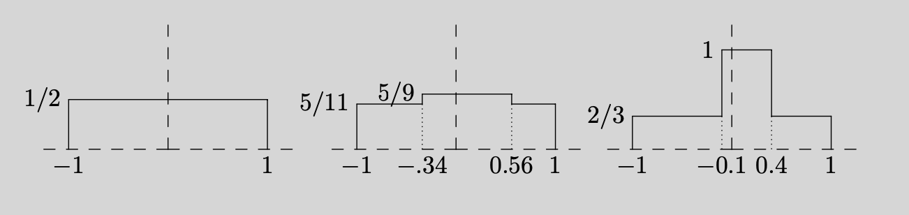
Figure 1: The probability distribution functions for $\mu_{0}^{0.5,0.2}$, $\mu_{.1}^{0.5,0.2}$, and $\mu_{.5}^{0.5,0.2}$ respectively.

Where $B_{r}[x]$ is the open ball of radius $r$ around $x$ and $\mathcal{L}|_{I}$ is Lebesgue measure restricted to the set $I$. See Figure 1 for a visualization since although the notation is cumbersome the images are relatively simple. The first formulation will be used to show these are indeed one dimensional geodesics and the second will be more natural when we wish to write these as projected measures. To see these are 1 dimensional geodesics we will use the following standard facts and notation about 1 dimensional transport problems.

Notation 2.1.

(1) The cumulative distribution function (cdf) $F_{\mu}(t):=\mu((-\infty,t))$.
(2) The ‘generalized inverse’ of the cdf is $F_{\mu}^{\circ}(s):=\sup\{x\in\mathbb{R}:F_{\mu}(x)\leq s\}$ for $s\in[0,1]$.

Theorem 2.2.

(Theorem 6.0.2 in [1]) Let $\mu$, $\nu$ be in $\mathcal{P}_{p}(\mathbb{R})$ and let $c(x,y)=|x-y|^{p}$ which is convex, non-negative, and has p-growth. If $\mu$ has no atoms, then $F_{\nu}^{\circ}\circ F_{\mu}$ is an optimal transport map from $\mu$ to $\nu$ for $1\leq p<+\infty$, and it is unique when $1<p<+\infty$.

If $\mu^{\alpha,\beta}_{0}=\mu=\frac{1}{2}\mathcal{L}_{[-1,1]}$ and $\nu=\mu^{\alpha,\beta}_{1}=\frac{\alpha}{2}\mathcal{L}_{[-1,1]}+(1-\alpha)\delta_{\beta}$, then $\mu$ has no atoms and

$$F_{\mu}(s)=\begin{cases}0&s<-1\\ \frac{1}{2}(s+1)&-1\leq s\leq 1\\ 1&s>1\end{cases},$$

$$F_{\nu}(s)=\begin{cases}0&s<-1\\ \frac{1-\alpha}{2}(s+1)&-1\leq s<\beta\\ \frac{1-\alpha}{2}(s+1)+\alpha&\beta\leq s\leq 1\\ 1&s>1\end{cases}$$

and,

$$F^{\circ}_{\nu}(s)=\begin{cases}-1+\frac{2}{1-\alpha}s&s<\frac{(1+\beta)(1-\alpha)}{2}\\ \beta&\frac{(1+\beta)(1-\alpha)}{2}\leq s\leq\frac{(1+\beta)(1-\alpha)}{2}+\alpha\\ -1+\frac{2}{1-\alpha}(s-\alpha)&s>\frac{(1+\beta)(1-\alpha)}{2}+\alpha\end{cases}.$$

We can put these together to get the transport map

$$F^{\circ}_{\nu}\circ F_{\mu}(s)=\begin{cases}-1&s<-1\\ -1+\frac{s+1}{1-\alpha}&-1\leq s<(1+\beta)(1-\alpha)-1\\ \beta&(1+\beta)(1-\alpha)-1\leq s<(1+\beta)(1-\alpha)-1+2\alpha\\ -1+\frac{s+1-2\alpha}{1-\alpha}&(1+\beta)(1-\alpha)-1+2\alpha\leq s\leq 1\\ 1&s>1\end{cases}.$$

We can then check that

$$\lambda F^{\circ}_{\nu}\circ F_{\mu}+(1-\lambda)\leavevmode\hbox to4.67pt{\vbox to7.51pt{\text{[drawing]}}}=\begin{cases}-\lambda+(1-\lambda)s&s<-1\\ \lambda\frac{\alpha}{1-\alpha}+s(1+\lambda(\frac{1}{1-\alpha}-1))&-1\leq s<\beta-\alpha(1+\beta)\\ \lambda\beta+(1-\lambda)s&\beta-\alpha(1+\beta)\leq s<\beta+\alpha(1-\beta)\\ \lambda\frac{-\alpha}{1-\alpha}+s(1+\lambda(\frac{1}{1-\alpha}-1))&\beta+\alpha(1-\beta)\leq s\leq 1\\ \lambda+(1-\lambda)s&s>1\end{cases}.$$

Where is the identity map. Note we simplified the conditions on $s$ and also collected the terms in $s$ to it is more clear what the push forward is of uniform measure,

$$\mu^{\alpha,\beta}_{0}=(\lambda F^{\circ}_{\nu}\circ F_{\mu}+(1-\lambda)\leavevmode\hbox to4.67pt{\vbox to7.51pt{\text{[drawing]}}})_{\sharp}\mu^{\alpha,\beta}_{0}=\mu^{\alpha,\beta}_{\lambda}$$

(replace the $\lambda$ with a $t$ and take the reciprocal of the term in front of $s$, the factor of $1/2$ comes from the fact we are pushing forward Lebesgue measure weighed by $1/2$). We can check locations of the jumps in the pdf of $\mu_{\lambda}^{\alpha,\beta}$ by looking at the images of the points where the piece-wise definition changes which are $\lambda\beta+(1-\lambda)(\beta-\alpha(1+\beta))=\beta-\alpha(1-\lambda)(1+\beta)$ and $\lambda\beta+(1-\lambda)(\beta+\alpha(1-\beta))=\beta+\alpha(1-\lambda)(1-\beta)$ which are the boundary points of $B_{\alpha(1-\lambda)}(\beta-\alpha\beta(1-\lambda))$.

Since each $\mu^{\alpha,\beta}_{t}$ is given by the push forward of a convex combination of the optimal transport map and the identity we can see that these are indeed 1 dimensional Wasserstein geodesics by theorem 7.2.2 in [1]. Furthermore, we know they are constant speed geodesics and so we can note that $W_{p}(\mu^{\alpha,\beta}_{t},\mu^{\alpha,\beta}_{s})=|t-s|W_{p}(\mu^{\alpha,\beta}_{0},\mu^{\alpha,\beta}_{1})$ which we can compute using the transport map:

$$W_{p}^{p}(\mu^{\alpha,\beta}_{0},\mu^{\alpha,\beta}_{1})=$$

$$\int_{-1}^{\beta-\alpha(1-\beta)}\Big{|}\frac{\alpha(1+s)}{1-\alpha}\Big{|}^{p}\frac{ds}{2}+\int_{\beta-\alpha(1-\beta)}^{\beta+\alpha(1+\beta)}\Big{|}\beta-s\Big{|}^{p}\frac{ds}{2}+\int_{\beta+\alpha(1+\beta)}^{1}\Big{|}\frac{\alpha(s-1)}{1-\alpha}\Big{|}^{p}\frac{ds}{2}$$

$$=\frac{1}{2(p+1)}\Big{[}\frac{\alpha^{p}}{(1-\alpha)^{p}}\Big{(}|1+\beta-\alpha(1-\beta)|^{p+1}+|\beta+\alpha(1+\beta)-1|^{p+1}\Big{)}\Big{]}$$

$$+\frac{1}{2(p+1)}\Big{[}(\alpha(1+\beta))^{p+1}+(\alpha(1-\beta))^{p+1}\Big{]}.$$

Note that when $\beta=0$ this formula simplifies greatly to $\frac{1}{p+1}\alpha^{p}$, thus we have $W_{p}(\mu^{\alpha,0}_{t},\mu^{\alpha,0}_{s})=\frac{\alpha}{(p+1)^{1/p}}|t-s|$ for $1\leq p<+\infty$, we can next use the fact that these measures are compactly supported and that $W_{\infty}(\mu,\nu)=\lim_{p\rightarrow+\infty}W_{p}(\mu,\nu)$ to see that $W_{\infty}(\mu^{\alpha,0}_{t},\mu^{\alpha,0}_{s})=\alpha|s-t|$ and so it is geodesic for $1\leq p\leq+\infty$. We now have sufficiently computed the one dimensional Wasserstein flows that we will reference when discussion sliced Wassertien geodesics.

3 Sliced Wasserstein Geodesics

The phenomena that we will be studying occurs naturally in three dimensions, but by considering embedding of $\mathbb{R}^{3}$ in higher dimensional spaces we get similar effects. Let $\mathbb{R}^{d}$ have an orthonormal basis $e_{1},e_{2},\cdots e_{d}$. We will use the following notation for surface (ie 2-dimensional) measure restricted to a spherical shell in a 3 dimensional subspace as well as some simple maps we will want to pushforward with.

Notation 3.1.

(1) For $d\geq 3$, $r>0$ and $x\in\mathbb{R}^{d}$ define

$$\sigma_{r,x}:=\frac{\mathcal{H}^{2}|_{\{ae_{1}+be_{2}+ce_{3}+x:a^{2}+b^{2}+c^{2}=r^{2}\}}}{\mathcal{H}^{2}(\{ae_{1}+be_{2}+ce_{3}:a^{2}+b^{2}+c^{2}=r^{2}\})}\hskip 20.00003pt\sigma_{0,x}:=\delta_{x}.$$

(2) For $a\in\mathbb{R}$, define the map $M^{a}:\mathbb{R}^{d}\rightarrow\mathbb{R}^{d}$ where $M^{a}(x)=ax$.
(3) Fox $x\in\mathbb{R}^{d}$ define the map $A^{x}:\mathbb{R}^{d}\rightarrow\mathbb{R}^{d}$ by $A^{x}(y)=x+y$.

Calculus and surfaces of revolution will confirm that

$$R^{\theta}_{\sharp}\sigma_{r,x}=\frac{1}{2r}\mathcal{L}|_{[\theta\cdot x-r(\theta\cdot x-rs(\theta),\theta\cdot x+rs(\theta)]}$$

where $s(\theta)=\sqrt{\sum_{i=1}^{3}(e_{i}\cdot\theta)^{2}}$ that is the norm of $\theta$ projected onto $\textup{span}\{e_{1},e_{2},e_{3}\}$. Fix $x\in\overline{B_{1}(0)}$, we will consider the following family of measures in $\mathbb{R}^{d}$,

$$\nu^{\alpha,x}_{t}=\frac{1}{(1-t+t(1-\alpha)^{-1})}\sigma_{1,0}+\frac{\alpha(-t+t(1-\alpha)^{-1})}{(1-t+t(1-\alpha)^{-1})}\sigma_{\alpha(1-t),x(1-\alpha(1-t))}.$$

$$\nu^{\alpha,x}_{0}=\sigma_{1,0}\hskip 30.00005pt\nu^{\alpha,x}_{1}=(1-\alpha)\sigma_{1,0}+\alpha\delta_{x}.$$

What is most important is that from this we get that $R^{\theta}_{\sharp}\nu^{\alpha,x}_{t}=M^{s(\theta)}_{\sharp}\mu^{\alpha x\cdot\theta}_{t}$, that is $t\mapsto\nu^{\alpha,x}_{t}$ is a sliced Wasserstein (extrinsic) geodesic because each projection is a Wasserstein geodesic. Note, this uses the fact that if $\mu_{t}$ is a geodesic then so is $M^{r}_{\sharp}\mu_{t}$.

Remark 3.2.

Note that $\textup{spt}(\nu_{t}^{\alpha,0})\subset\partial B_{1}(0)\cup\partial B_{\alpha(1-t)}(0)$ which is disconnected. We can note that the total mass in $\partial B_{1}(0)$ is $1-\alpha t$ and the total mass in $B_{\alpha}(0)$ is $t\alpha$. The fact this is changing in time is an example of the fact that if one attempted to follow the measures on the particle level, they would hop between these connected components and not move continuously. Note that [6] shows this phenomena can occur with absolutely continuous curves in remark 3.9. The example given here is notable since it is the first example of this pathological ‘hopping’ occurring with a curve as nice as a geodesic.

We should note that we can quickly grow this family of Sliced Wasserstein geodesics by adding dilation and translations. It is a fact that if $t\mapsto\mu_{t}$ is a Wasserstein geodesic in $\mathbb{R}$, then $t\mapsto M^{a}_{\sharp}(\mu_{t})$ and $t\mapsto A^{ty+z}_{\sharp}(\mu_{t})$ are also geodesics for $a\in\mathbb{R}$ and $z,y\in\mathbb{R}$. As such, the restriction of around the origin and having unit radius are simply to reduce notation. Thus for all $\alpha\in(0,1)$, $a\in\mathbb{R}$, $x\in\overline{B_{1}(0)}$ and $y,z\in\mathbb{R}^{d}$, we can note that $t\mapsto M^{a}_{\sharp}(A^{ty+z}_{\sharp}(\nu^{\alpha,x}_{t}))$ are $SW_{p,q}$ geodesics. Note that the edge cases when $\alpha=0$ and $\alpha=1$ are also Sliced Wasserstein geodesics, they are translations when $\alpha=0$ and pure dilation when $\alpha=1$, these are also Wasserstein geodesics and as such were of less interest to the author. Thus, we have found more than one interesting Sliced Wasserstein geodesic, we have actually found a five parameter family, showing that the dimension of the space of sliced Wasserstein geodesics which are not Wasserstein geodesics is at least $3d+2$ for any particular embedding of $\mathbb{R}^{3}$ into $\mathbb{R}^{d}$.

The barycenter and gradient flow problems were referenced in the abstract. Note that geodesics are a simple case of both of these (eg finding the barycenter of measures along the geodesic and gradient flow of the distance functional). These examples demonstrate different behavior of the Wasserstein and Sliced Wasserstein metrics. One difference is that these geodesics show that the Sliced Wasserstein see movement to the ‘interior’ of a shell as closer than the Wasserstein metric. This means, at least in some cases, the Sliced Wasserstein metric will lose mass on the periphery faster along gradients and barycentric flows. Furthermore, these flows no longer correspond to continuous movement on the particle level, which is often said to make Wasserstein flows ‘intuitive’. These qualitative differences in the flows should be kept in mind when opting to replace a Wasserstein metric with a sliced Wasserstein metric. A potential area of future research could be to quantify these differences.

4 Non-equivalence of metrics

We will now use these geodesics to prove the following version of Main Theorem (3) from [5] which was a strengthening of Theorem 2.1(iii) and correction of Theorem 2.1(ii) in [2]. Note that there are some cases, particularly when $p=1$ that are shown in [2] and [5] that are not shown here so this is not a strict strengthening, but we do cover all the remaining cases. This is the first paper as far as the author is aware to address the case when $p=+\infty$ so in addition cases left out by [2] and [5] this edge case has finally been addressed. Attention should be drawn to the proof method which is distinct from the previous papers. Instead of using a probabilistic method which only proved examples exist this paper provides direct proof by constructing specific examples. Additionally, the examples given are all uniformly bounded support, something done in [5] for only $p\geq 2$ and finite $q$, showing that bi-Lipschitz equivalence cannot be recovered by restricting to measures restricted to an arbitrary compact set.

Theorem 4.1.

For $d=2$, $1\leq p\leq+\infty$ and $1\leq q<+\infty$, $p=1$ and $q=+\infty$, or for $d\geq 3$ $1\leq p,q\leq+\infty$, $(\mathcal{P}_{p}(\mathbb{R}^{d}),SW_{p,q})$ and $(\mathcal{P}_{p}(\mathbb{R}^{d}),W_{p})$ are not bi-Lipschitz equivalent.

Proposition 4.2.

For all $1<p\leq+\infty$ and $1\leq q\leq+\infty$ and $d\geq 3$, $d\in\mathbb{N}$, the spaces $(\mathcal{P}_{p}(\mathbb{R}^{d}),W_{p})$ and $(\mathcal{P}_{p}(\mathbb{R}^{d}),SW_{p,q})$ are not bi-Lipschitz equivalent nor are they equivalent along geodesics in $(\mathcal{P}_{p}(\mathbb{R}^{d}),SW_{p,q})$.

Proof of Proposition 4.2.

Consider the family of measures $\nu_{t}^{\alpha,0}$ for $t>0$ and $\nu_{0}^{\alpha,0}$. We have shown above that

$$SW_{p,q}(\nu_{t}^{\alpha,0},\nu_{0}^{\alpha,0})=\left[\frac{1}{\mathcal{H}^{d-1}(\mathbb{S}^{d-1})}\int_{\mathbb{S}^{d-1}}\Big{(}W_{p}(R_{\sharp}^{\theta}\nu_{t}^{\alpha,0},R_{\sharp}^{\theta}\nu_{0}^{\alpha,0})\Big{)}^{q}d\mathcal{H}^{d-1}(\theta)\right]^{1/q}$$

$$=\left[\frac{1}{\mathcal{H}^{d-1}(\mathbb{S}^{d-1})}\int_{\mathbb{S}^{d-1}}\Big{(}W_{p}(M^{s(\theta)}_{\sharp}\mu_{t}^{\alpha,0},M^{s(\theta)}_{\sharp}\mu_{0}^{\alpha,0})\Big{)}^{q}d\mathcal{H}^{d-1}(\theta)\right]^{1/q}$$

$$=\left[\frac{1}{\mathcal{H}^{d-1}(\mathbb{S}^{d-1})}\int_{\mathbb{S}^{d-1}}\Big{(}s(\theta)t\frac{\alpha}{(1+p)^{1/p}}\Big{)}^{q}d\mathcal{H}^{d-1}(\theta)\right]^{1/q}$$

$$=\frac{\alpha t}{(p+1)^{1/p}}\left[\frac{1}{\mathcal{H}^{d-1}(\mathbb{S}^{d-1})}\int_{\mathbb{S}^{d-1}}\Big{(}s(\theta)\Big{)}^{q}d\mathcal{H}^{d-1}(\theta)\right]^{1/q}=\frac{\alpha t}{(p+1)^{1/p}}C_{d,q}.$$

We can note that $C_{d,q}=\left[\frac{1}{\mathcal{H}^{d-1}(\mathbb{S}^{d-1})}\int_{\mathbb{S}^{d-1}}\Big{(}s(\theta)\Big{)}^{q}d\mathcal{H}^{d-1}(\theta)\right]^{1/q}$ is just some dimensional constant depending on $q$, $0\leq s(\theta)\leq 1$ and it is non-zero on a set of positive measure so we can note that $0<C_{d,q}\leq 1$, it is clear when $q=+\infty$ that $C_{d,q}=1$.

On the other hand, we can compute $W_{p}(\nu_{t}^{\alpha,0},\nu_{0}^{\alpha,0})$, the map $T:\mathbb{R}^{d}\rightarrow\mathbb{R}^{d}$ where $T(x)=\frac{x}{|x|}$ for $x\neq 0$ and $T(0)=0$ has c-monotone graph for all $c(x,y)=|x-y|^{p}$ $1\leq p<+\infty$ and so by 6.1.4 in [1] we know that this is an optimal transport map from $\nu_{t}^{\alpha,0}$ to $\nu_{0}^{\alpha,0}$ for $0<t<1$ and since it is for all $1\leq p<+\infty$ we can by taking limits argue it is optimal for $p=+\infty$. We can then compute:

$$W_{p}^{p}(\nu_{t}^{\alpha,0},\nu_{0}^{\alpha,0})=\int|T(x)-x|^{p}d\nu_{t}^{\alpha,0}(x)=\int_{B_{1}(0)}[1-\alpha(1-t)]^{p}d\nu_{t}^{\alpha,0}$$

$$=\frac{\alpha t}{(1-\alpha(1-t))}[1-\alpha(1-t)]^{p}=\alpha t(1-\alpha(1-t))^{p-1}.$$

We can then see that $\frac{W_{p}(\nu_{t}^{\alpha,0},\nu_{0}^{\alpha,0})}{SW_{p,q}(\nu_{t}^{\alpha,0},\nu_{0}^{\alpha,0})}=\frac{(1-\alpha(1-t))^{1-1/p}(p+1)^{1/p}}{C_{d,q}}(\alpha t)^{\frac{1}{p}-1}$. When $1<p<+\infty$ clearly for $p>1$ this expression goes to $+\infty$ as $t\rightarrow 0$ for all fixed $\alpha$ and so we have that $W_{p}$ and $SW_{p,q}$ are not bi-Lipschitz equivalent.

The case when $p=+\infty$ we can note that $W_{\infty}(\nu_{t}^{\alpha,0},\nu_{0}^{\alpha,0})=1-t(1-\alpha)$ and $SW_{\infty,q}(\nu_{t}^{\alpha,0},\nu_{0}^{\alpha,0})=\alpha tC_{d,q}$, we can see that $\lim_{t\rightarrow 0}\frac{W_{\infty}(\nu_{t}^{\alpha,0},\nu_{0}^{\alpha,0})}{SW_{\infty,q}(\nu_{t}^{\alpha,0},\nu_{0}^{\alpha,0})}=+\infty$.

∎

Note that it is not known if the exponents here are optimal, we have here that $t\mapsto\nu_{t}^{\alpha,0}$ are Lipschitz in $SW_{p,q}$ but only $\frac{1}{p}$-Hölder continuous with respect to $W_{p}$. One corollary of theorem 5.1.5 in [4] is that every Lipschitz path (and so every geodesic) in $SW_{p,q}$ in $\mathbb{R}^{d}$ is at least $\frac{1}{p(d+1)}$-Hölder continuous. Thus, as far as the author is aware, it is unclear what is the optimal exponent $\alpha$ such that every Lipschitz path and every geodesic in $SW_{p,q}$ are $\alpha$-Hölder continuous with respect to $W_{p}$ or if the exponents for Lipschitz paths and geodesics are different.

The addendum about along geodesics in Proposition 4.2 means that this theorem can also be applied to show facts about the intrinsic metric of $\mathcal{P}^{n}(\mathbb{R}^{d})$. There was some hope (for instance [3]) in the community that the non-equivalence could be fixed by considering the intrinsic metric, that is the metric where the distance between two points is the length of the shortest path between them (see [6] for example for more details). Unfortunately since the intrinsic and extrinsic metrics agree along extrinsic geodesics we get the immediate corollary.

Definition 4.3.

We define the $SW_{p,q}$ intrinsic metric,

$$\ell_{SW_{p,q}}=\inf_{\{\mu_{t}\}_{t\in[0,1]}\in AC(\mathcal{P}_{p}(\mathbb{R}^{d}),SW_{p,q})}\Bigg{(}\sup_{0=t_{0}<\dots<t_{n}=1;n\in\mathbb{N}}\sum_{i=0}^{n-1}SW_{p,q}(\mu_{t_{i}},\mu_{t_{i+1}})\Bigg{)}.$$

Corollary 4.4.

If $d\geq 3$ and $1<p\leq+\infty$ and $1\leq q\leq+\infty$, then $(\mathcal{P}_{p}(\mathbb{R}^{d}),\ell_{SW_{p,q}})$ and $(\mathcal{P}_{p}(\mathbb{R}^{d}),W_{p})$ are not bi-Lipschitz equivalent.

Proof.

If $t\mapsto\nu_{t}^{\alpha,0}$ is an extrinsic geodesic with respect to $SW_{p,q}$, that is $SW_{p,q}(\nu_{t}^{\alpha,0},\nu_{s}^{\alpha,0})=|s-t|SW_{p,q}(\nu_{0}^{\alpha,0},\nu_{1}^{\alpha,0})$, then it is a standard fact around these constructions that $\ell_{SW_{p,q}}(\nu_{t}^{\alpha,0},\nu_{s}^{\alpha,0})=SW_{p,q}(\nu_{t}^{\alpha,0},\nu_{s}^{\alpha,0})$. Thus, the comparisons done in proposition 4.4.2 between $SW_{p,q}$ and $W_{p}$ are the same as the comparisons between $\ell_{SW_{p,q}}$ and $W_{p}$, so the latter are not bi-Lipchitiz equivalent.

∎

In the introduction, it was promised that this paper would fill the gaps left by [5] and [2]. As of yet this has not fully been done, there remains to show the cases where $d=2$, $p=+\infty$, we will show this case separately.

Lemma 4.5.

For $d=2$ where $p=+\infty$ and $1\leq q\leq+\infty$ or $+\infty>p>1$ and $q=+\infty$ then $(\mathcal{P}_{p}(\mathbb{R}^{d}),W_{p})$ and $(\mathcal{P}_{p}(\mathbb{R}^{d}),SW_{p,q})$ are not bi-Lipschitz equivalent.

Proof.

First for $p=+\infty$ consider the family of measures $\mu_{t}=t\delta_{0}+(1-t)\frac{\mathcal{H}^{1}|_{\partial(B_{1}(0)}}{2\pi}$. Note that $W_{\infty}(\mu_{0},\mu_{t})=1$ for all $0<t\leq 1$. Furthermore, note that $R^{\theta}_{\sharp}\frac{\mathcal{H}^{1}|_{\partial(B_{1}(0)}}{2\pi}$ has the distribution function $\frac{1}{\pi\sqrt{1-x^{2}}}$ call this measure $\nu$. We can then note that the optimal transport map, $T$ between $t\delta_{0}+(1-t)\nu$ and $\nu$ (that is between $R^{\theta}_{\sharp}\mu_{t}$ and $R^{\theta}_{\sharp}\mu_{0}$) is monotone. Note that while $\int_{-s}^{s}\frac{1}{\pi\sqrt{1-x^{2}}}<t$, we can note that $T(s)=0$ and so $|T(s)-s|$ is increasing ($s>0$), but when $\int_{-s}^{s}\frac{1}{\pi\sqrt{1-x^{2}}}>t$ $s\mapsto|T(s)-s|$ is decreasing ($s>0$). Thus, we can find $W_{\infty}(R^{\theta}_{\sharp}\mu_{t},R^{\theta}_{\sharp}\mu_{0})$ to be this maximum which is at $s=\frac{2\sin(t)}{\pi}$. We can then note that due to the spherical symmetry of $\mu_{t}$ we know that $SW_{\infty,q}(\mu_{t},\mu_{0})=W_{\infty}(R^{\theta}_{\sharp}\mu_{t},R^{\theta}_{\sharp}\mu_{0})=\frac{2\sin(t)}{\pi}$ (this is regardless of the choice of $q$ due to the spherical symmetry). Thus, we can note that $\lim_{t\rightarrow 0}\frac{W_{\infty}(\mu_{t},\mu_{0})}{SW_{\infty,q}(\mu_{t},\mu_{0})}=+\infty$, and so we have shown these are not bi-Lipschitz equivalent.

∎

Proof of Theorem 4.1.

Proposition 4.2 covers $d\geq 3$ and $p\neq 1$ and lemma 4.5 covers $d=2$ and $p=+\infty$. We can then note that [5] Main theorem (3) handles $d\geq 3$ $p=1$ and any $q$ as well as $d=2$, $1<p<+\infty$ and $1\leq q<+\infty$ as well as $p=1$ with $q=+\infty$.

∎

We should note that at this point, the math community almost has an if and only if characterization of the equivalence of these metrics, the only remaining cases are $d=2$ with $1<p<+\infty$ and $q=+\infty$.

5 Acknowledgements

I am greatly indebted to Wilfrid Gangbo who taught me optimal transport theory, guided me to sliced Wasserstein metrics, and advised me during the process of writing and research. I would also like to that Jun Kitagawa for fruitful discussion particularly about how to get results in higher dimensions. This work was partially supported by the Air Force Office of Scientific Research under Award No. FA9550-18-1-0502.

References

- [1] Ambrosio, L.; Gigli N.; and Savaré G. “Gradient Flows in Metric Spaces and in the Space of Probability Measures” Second Edition, Lectures in Mathematics ETH Zürich (2008).
- [2] Bayraktar, E. and Gaoyue G. “Strong equivalence between metrics of Wasserstein type,” Electronic Communications in Probability, Electron. Commun. Probab. 26, 1-13, (2021)
- [3] Bonet, C., et al. “Efficient gradient flows in sliced-Wasserstein space.” arXiv preprint arXiv:2110.10972 (2021).
- [4] Bonnotte, N. “Unidimensional and evolution methods for optimal transportation,” Ph.D. thesis (2013). http://cvgmt.sns.it/paper/2341/.
- [5] Kitagawa, J., and Asuka T. “Sliced optimal transport: is it a suitable replacement?” arXiv preprint arXiv:2311.15874 (2023).
- [6] Park, S., and Slepčev D. “Geometry and analytic properties of the sliced Wasserstein space.” arXiv preprint arXiv:2311.05134 (2023).