A Toy Model for the 2/3 Fractional Quantum Hall edge channel
Abstract
We present a minimal model capturing the intriguing physics of the fractional quantum Hall state at filling factor . Inserting fictive reservoirs —either Landauer Reservoirs (LRs) or Energy Preservings Reservoirs (EPRs) —along the counter-propagating modes to mimic edge channel mixing, the conductance is shown rapidly converging towards the Kane-Fisher-Polchinski conductance fixed point ) for both EPRs and LRs. However, LRs give equal charge and thermal relaxation lengths while EPRs show infinite thermal relaxation length. The Hall bar current noise is found varying linearly with current at large bias, leading to an apparent (or Fake) Fano factor for N LRs, or exponentially vanishing for EPRs. Withal, inserting a Quantum Point Contact in the middle of the Hall bar reveals the recently observed conductance plateau. Finally, the 2010 Bid et al. first reported observation of neutral modes can be explained by an upstream diffusive heat flow and delta-T noise, without introducing any specific collective neutral mode.
The Fractional Quantum Hall Effect (FQHE) arises in 2D electron system (2DES) under high perpendicular magnetic field , at low temperature, when the filling factor value is fractional — being the electron density. At simple rational values of , the 2DES forms topologically insulating states. Conduction occurs on the edge via topological chiral edge channels. For , i.e. , , , …, there are p co-propagating edge channels. For , with , counter-propagating edge channels occur. Early theoretical work [1, 2] modelled the edge by an outer chiral integer edge channel, conductance and an inner counter-propagating fractional edge channel with conductance ). However, this picture gives a total conductance of ) while all observations find ). Solving this puzzle, the Kane-Fisher-Polchinski (KFP) model [3, 4] showed, in a Chiral Luttinger Liquid (CLL) picture, that the combination of Coulomb coupled counter-propagating modes with spatially random disorder on the edges leads to a downstream chiral charge mode with conductance and a bosonic upstream neutral mode. Later, experiments led by the Weizmann group using current noise measurements [5] found evidence of upstream excitation, therefore assigned to the predicted neutral mode. The puzzling physics of the edge has then led to a flurry of theoretical models [6, 7, 8, 9, 10, 11, 12, 13, 14] inspired by the KFP model to improve it or to adapt it to situations where more complex reconstruction of the edge occurs [15, 16]. Concurrently experimental works based on conductance, noise, or thermal conductance have explored the nature of the edge [17, 18, 19, 20, 21, 22, 23, 24, 25]. Recently, artificial counter-propagating edge channels have been realised by coupling left and right regions of different ( and ) filling factor [26, 27, 25]. However the KFP model, although widely accepted, lacks of physical intuition for non-experts. It is difficult to separate what comes from the bosonic modes entering in the CLL picture with what comes from the disorder which mixes the counter-propagating modes by tunnelling.
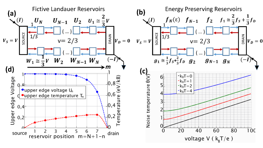
Here we provide a novel approach using basic tools of mesoscopic physics. The model discussed in the following should be better viewed as a Toy model. It is not intended to provide a microscopic description of channel mixing; it aims at exploring, in an easy way, what are the minimal ingredients leading to results compatible with observations. We consider a Hall bar, with physical source and drain ohmic contacts on the left and right ends, see Fig.1(a) and (b). In this Toy model, N fictitious charge reservoirs are inserted along the upper and lower edges to enable charge equilibration between counter-propagating channels. Note that, by using reservoirs, we do not address a third possible the regime: coherent channel mixing[28, 27]. We consider two generic cases schematically shown in Fig.1. In Fig.1(a), the reservoirs are fictive ohmic contacts described as Landauer reservoirs (LR). In Fig.1(b) the reservoirs are Energy-Preserving Reservoirs (EPR), as introduced in [29]. In both cases, the and outer and inner channels ballistically propagate between two consecutive reservoirs. We recall that, for a LR, quasiparticles are absorbed whatever their energy and are emitted following a Fermi distribution having the temperature and the chemical potential of the reservoir (here expressed in voltage units). LRs thus provide full equilibration of both charge and energy between the counter-propagating channels. An opposite situation occurs for EPRs: an excitation hitting the reservoir at energy is absorbed and re-emitted at the same energy and charge equilibration alone occurs.
In the following, we find that both LRs and EPRs lead to the same conductance values for reservoirs, rapidly converging with towards the KFP conductance fixed point. The case of energy preserving scatters was overlooked in the literature and our result shows that dissipative processes are not necessary to reach the KFP conductance fixed point. However, beyond conductance, comparing LRs and EPRs leads to quantitatively different temperature distribution and current noise.
We first concentrate on predictions for conductance and current noise for a Hall bar for both LRs and EPRs.
For LRs, the evenly distributed fictive contacts are floating at potential () along the upper (lower) edge with no external current entering them. For convenience we set the conductance quantum equal to unity. The Landauer-Büttiker relation For the fictive reservoir on the upper edge channel is:
| (1) |
A similar relation holds for the potentials of the lower edge. For energy preserving reservoirs:
| (2) |
with the non-equilibrium energy distribution of the EPR of the upper edge channel. A similar set of equations holds for the energy distributions of the lower edge channel. Using appropriate Landauer-Büttiker boundary conditions on source and drain contacts at potential and respectively, we find the following voltage distribution for LRs (see the Supplemental Material (SM)):
| (3) |
with . Similarly, the energy distribution for the EPRs is:
| (4) |
with the Fermi distributions of the source (drain) contacts at temperature and voltage ( respectively. For the lower edge channel, exchanging source and drain voltages (energy distributions) in equations 3(4) leads to similar expressions for (or ). The conductance for reservoirs is found to be:
| (5) |
for both LRs and EPRs. In general, as long as conductance properties are concerned, both dissipative and non-dissipative reservoirs remarkably give the same conductance. The first five values of when goes from to are respectively: , , , , and . With just two fictive reservoirs the KFP conductance fixed point is reached within accuracy. It is interesting to compare the current flowing through the upper and lower edge channel. For the upper edge we find a downstream current converging towards :
| (6) |
while for the lower edge we find an upstream current exponentially vanishing with :
| (7) |
We now concentrates on the case of dissipative Landauer reservoirs to investigate dissipation and noise. For simplicity we set the voltages and . Along the upper channel, from left to right, we observe from Eq.3 that the voltages remain almost equal to all along the channel and drops rapidly to near the drain contact, see Fig.1(d). Reciprocally, from right to left, the lower channel voltage remains almost zero and rapidly rise to near the source. This feature has several implications: we expect strong dissipation near the drain (source) for the upper (lower) edge and almost no dissipation along the Hall bar. Indeed we find that the power dissipated in the nth upper edge fictive contact is (see SM): . For the lower edge, the power . This confirms the existence of ”hot spots” near the drain and the source for respectively the upper and lower edge channel, as found in previous theoretical models [6, 9, 10] . To check that the calculated power expressions make sense, we have computed, see SM, the total power in the Hall bar, summing the drain, the source, and the upper and lower edge contributions. We find a total power as it should be. Knowing the set of , we can calculate the temperature distribution () for the upper (lower) edge channel using the universal quantum thermal conductance , being the Lorenz number. Equal thermal conductance for the and channels was predicted in [30] and experimentally found in [18, 20, 23]. Fixing the temperature of the physical drain and source reservoirs equal to , the temperature of the fictive reservoirs is obtained by solving the standard heat flow equations (see SM). The solution is:
| (8) |
The same temperature distribution is found for the lower edge. For the upper edge , from right to left, we observe a square root like increases of the spatial temperature distribution followed by a sudden drop to near the drain, see Fig.1(d). A similar symmetric spatial variation occurs for the lower edge. Importantly, the increase of the temperature all along the edge channel signals a diffusive upstream heat flow contrasting with the downstream charge flow. As our model does not require introducing a specific neutral collective mode, the counter-propagating heat flow plays its role. Our Toy model provides thus a new perspective on the nature of the neutral mode.
Knowing the temperature distribution along the edge of the Hall bar, we now can compute the non equilibrium hot electron thermal noise for . To proceed, we consider all independent thermal current noise sources generated between each pair of fictive reservoirs. For the pair on the upper edge the current noise spectral density is with the given by Eq.8. A fluctuation between a fictive contact pair is found giving rise to the fluctuation at the source contact and, from current conservation, an equal fluctuation in the drain contact. Adding the uncorrelated mean square fluctuations of the noise of all pairs provides the total drain current noise. Setting source and drain temperatures to for clarity, we find the total current noise power, can be expressed as:
| (9) |
with the (fake) Fano factor given by (see SM):
| (10) |
Summation (10) is valid for large and gives . For large lengths, the non-equilibrium hot electron thermal noise vanishes like the square root of , the Hall bar length. Similar length dependence was predicted using different theoretical approaches [10, 31] and experimentally observed [25]. We observe from the summation in Eq.10 where stands for , that the main noise contributions do not comes from the ”hot spots” (near the drain for the upper edge) but from noise sources situated close to the source having the smallest noise temperature ( close to ). For finite temperature , the asymptotic linear variation of the noise with applied voltage becomes accurate for see Fig.1(c).
We now turn to the dissipation and the current noise for the case of energy preserving reservoirs instead of LRs. Because of the nature of the fictive EPRs, we do not expect any dissipation along the upper and lower channels except at source and drain which are physical LRs. Indeed, the sum of the power dissipated in the source and the drain is found equal to the Joule power , see SM. Thus, contrasting with the Landauer reservoir case where the thermal and charge equilibration lengths were found equal, the thermal length is here infinite. These two opposite thermal length behaviours have been experimentally observed [21, 32, 33]. For EPR, we expect a current noise different from the LR case. The non-equilibrium energy distribution and given by Eq.4, are in general between zero and one. This leads to fluctuations of the state occupation number at energy equal to . This results in the current noise spectral density associated to a EPR pair equal to : where we have defined the fictive temperatures
| 5 | 0,07911 | 0,1937 | 0,002698 | 0,6556 |
| 6 | 0,07305 | 0,1933 | 0,000908 | 0,6621 |
| 7 | 0,06827 | 0,1931 | 0,000304 | 0,6649 |
| 0 | 0.19298… | 0 | 2/3 |
The total noise observed in the drain or source can be calculated as we did above for LRs, replacing by . In contrast with the LR case, the noise is found exponentially vanishing with the size (see SM). The fictive temperatures growing linearly with , we can define the fake Fano factor . For large we found contrasting with . Such exponential dependence was reported in [33]. Table 1 gives Fano factor values for some finite values.
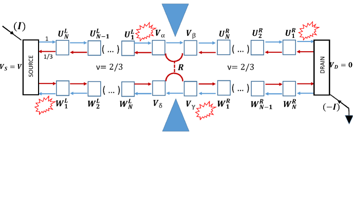
We now address practical situations exploiting the present Toy model. While we have considered above an homogeneous Hall bar, we now investigate the conductance when a quantum point contact is located in the middle of the Hall bar and induces tunnelling between the upstream upper and lower fractional inner edge channels while the downstream integer channel is transmitted. To proceed, we introduce fictive reservoirs on the left side of the QPC (both for the lower and upper edge) and, symmetrically, reservoirs on the right side, see Fig.2. We seek for a solution of the upper and lower potentials and respectively on the right (R) and left (L) side of the QPC. The boundary conditions, given by Landauer-Büttiker relations at the source and the drain and at the QPC, see SM, provide a determination of the unknown potentials. For large , the QPC conductance is found:
| (11) |
where is the reflection probability of the fractional inner channel The graph of QPC conductance versus is given in the SM. Interestingly, for full reflection we get the half conductance quantum . A similar result was found in [24] in a model attempting to explain the observed conductance plateau and in the theoretical works of reference [14, 34]. We find the same conductance for energy-preserving reservoirs instead of LRs, confirming that conductance alone can not distinguish between dissipative and non-dissipative regime.
It is interesting to look at the potential distribution along the edges for the LR case. Starting from the source contact at , the upper edge voltage remains almost equal to but quickly drops near QPC to reach . Then on the upper right of the QPC, starting at the voltages remain almost constant and rapidly drop near the drain at . Similarly, starting from the drain, the lower edge voltages remain almost zero and rapidly increase near the QPC to reach . On the left of the QPC, the voltages remain almost equal to to finally rapidly increase near the source to . The rapid drops of potentials being associated with dissipation we can identify two new ”hot spots” on both side of the QPC as shown in Fig.2.
As another application of the toy-model, we now consider the set-up of Fig.3, which is similar to Bid’s experiment reporting counter-propagating neutral modes [5]. Exploiting the results of [12] shows that neutral modes are unable to propagate more than very few charge relaxation lengths at all frequencies. Then, it is unlikely that the neutral mode can be the source of partition noise in experiment [5]. Here we show that the thermal gradient due to the counter-propagating heat flow fund above is responsible for the observed noise. In the set-up of Fig.3, the source contact (), located at the upper right of a QPC, is at potential and injects the current . The left and right contacts () and () of the Hall bar are grounded. A fourth physical contact () on the lower left side of the QPC records the voltage fluctuations , from which the current noise can be inferred.
For simplicity, and the QPC weakly backscatters the (-1/3) inner edge () leaving the Hall bar almost unperturbed. The Hall bar edges are modelled by fictive LRs. According to the above results, the current flows from () to contact (). A hot spot forms at () and on the left side of (). This generates an upstream heat flow flowing along the upper edge and heating the upper side of the QPC. For LRs between the QPC and (), the temperature of the upper channel at the QPC is, according to Eq. 8:
| (12) |
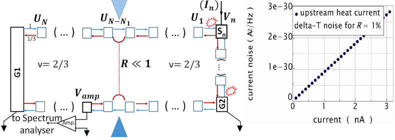
In contrast, the lower channel, connected to zero temperature zero voltage contacts remains at . This situation generates a ”delta-T” shot noise [35, 36, 37, 38] at the QPC whose one side is at and the other side at . A similar conclusion, but in a full CLL approach was found in [6]. is given by, see [36]:
| (13) |
where the (1/3) factor come from the tunnelling of quasiparticle of charge . For , zero temperature and transmission (), nA gives /Hz a value close to the reported experimental value. If LRs are now replaced by EPRs, the distribution function at the location of the QPC is close to the Fermi distribution of contact . Therefore no delta-T noise is expected.
To conclude, the present Toy model provides a novel and easy way to get intuition on the physics of the fractional edge. Generalisation to edges involving and channels yields similar results with . The model gives a new interpretation of neutral excitations as heat flow. A Bid type experiment observing noise would signal a dissipative equilibrium regime (i.e. LRs) generating Delta-T noise. In contrast, observing no noise would signal no thermal equilibration. Finally, we learned that the CLL physics is not the first step required to describe the 2/3 physics. Including capacitance to ground and mutual reservoir capacitances, may give a way to restore the yet neglected CLL physics and describe the AC regime [12, 39, 25].
We thank Ankur Das, Yuval Gefen, Moshe Goldstein, Sourav Manna, Carles Altimiras, Olivier Maillet, François Parmentier for useful discussions. We acknowledge the European Union H2020 research and innovation program under grant agreement No. 862683, “UltraFastNano”.
SUPPLEMENTAL MATERIAL
A1 Hall bar conductance for fictive LRs:
To compute the Hall bar conductance with LRs inserted between source and drain, we use Landauer-Büttiker relations. The boundary conditions are: a current sent by the external circuit enters the physical source contact and accordingly, a current enters the drain contact. The Voltages of the source (drain) contacts are () respectively. The fictive LR voltages are noted () for upper (lower) edges. We have:
| (14a) | |||
| (14b) | |||
| (14c) | |||
| (14d) | |||
with running from to following a counterclockwise (upstream) order. Seeking for a solution we find or . The general solution is a linear combination of these two solutions whose coefficient are determined by the source and drain boundary conditions 14a,14d, which leads to:
| (15) |
with . Using Eq.14d (or Eq. 14a) we find the conductance for N reservoirs, including the case .
To compute the temperature of each floating fictive reservoirs, we set the voltages and for simplicity and we first calculate the Joule power dissipated in each reservoir:
| (16) |
A similar calculation hold for the reservoir of the lower edge with power . To check that the power calculated makes sense, we compute the total power dissipated in the Hall bar in the limit . The Joule power dissipated at the drain and the source by the upper and the lower edge channels are respectively :
| (17) |
as it should be.
To obtain the temperature distribution along the edge, we have to solve the following heat flow equation:
| (18) |
As , the general solution can be written as where , , and are determined from the drain and source thermal boundary conditions. The solution, valid for large , is given by Eq. 8 in the main text. For small , values of are given in table 2 for and .
| N | |||||||
|---|---|---|---|---|---|---|---|
| 4 | 0,2297 | 0,2121 | 0,1747 | 0,1237 | |||
| 5 | 0,2345 | 0,2232 | 0,1949 | 0,1593 | 0,1126 | ||
| 6 | 0,2382 | 0,2310 | 0,2082 | 0,1805 | 0,1474 | 0,1042 | |
| 7 | 0,2409 | 0,2367 | 0,2177 | 0,1949 | 0,1688 | 0,1378 | 0,0974 |
Once we have the set of values, we can compute the (hot) thermal (chiral) current noise source between pair of reservoirs (n+1,n) on the upper edge and calculate, for each independent pairs, the induced source and drain fluctuations. A similar calculation is done for the lower edge. We found that the current noise viewed at the source contact due to the (n+1,n) pair is : . Adding all independent current noise of each pairs for both upper and lower edge and adding the drain and source contacts contributions, we get the total noise of the Hall bar. It is interesting to note the following. The hottest temperature for the upper (lower) edge occurs close to the drain (source), forming ”hot spots”.1 but the current noise contribution is exponentially suppressed by a factor. On the contrary the current noise sources close to the source (drain) contact contribute to with the largest weight while they have the lowest noise temperature. This corresponds to ”noise spots”. However, here no shot noise occurs in the present Toy model, only thermal noise with temperature rising linearly with . As the temperatures near the source scale as the non-equilibrium noise vanishes for large length.
We thus get the effective noise temperature of the whole 2/3 Hall bar defined as: , for N fictive probes when a drain-source voltage s applied. For zero drain and source temperature, . To characterise the noise, we define the effective (or fake) Fano factor by , i.e. .
Table 1, in the main text, gives values of the fake Fano factor. The values for N=5-7 result from an exact numerical calculation for reservoirs. We see that for the large limit given by Eq.10 is almost reached.
A2 Hall bar conductance for fictive EPRs:
The calculation of the unknown distributions and for the reservoir of the upper and lower edge is very similar to the calculation of potentials for LRs. The boundary conditions are the Fermi distribution and at respectively the source and drain reservoirs. We get the set of following linear equations for the upper edge:
| (19a) | |||
| (19b) | |||
| (19c) | |||
A similar set of equation holds for lower edge. The general solution is:
| (20) |
for , where, as above .
The non-equilibrium distribution are thus linear combination of the source and drain Fermi distributions. In the limit of large , , . Similarly, and . The current at the source is :
| (21) |
The conductance is thus insensitive to the nature of the reservoirs, LRs or EPRs.
We now investigate where dissipation occurs in the 2/3 Hall bar with EPRs. Because of the nature of the fictive BRs we do not expect any dissipation along the upper and lower channels except at source and the drain which are physical LRs. Indeed, lets calculate the power and dissipated in the source and in the drain. For simplicity we consider the reservoirs at zero temperature and chose the zero of energy at the chemical potential of the grounded drain contact. For large , we have:
| (22) |
A similar expression gives . The total Joule heating is and thus exclusively occurs in the physical ohmic drain and source contacts. The study of dissipation indicates that no generation of thermal current fluctuations can occurs in the fictive EPRs. However, the distribution , and can generate non thermal population fluctuations. We can define a fictive temperature associated wth the distribution and defined as:
| (23) |
There is an important difference between the for EPRs and the for LRs. While the latter have to obey the heat flow equation 18, the former are entirely defined by the . Figure 4 compares EPR and LR temperatures
The noise for the case of EPR reservoirs is computed in a way similar to the LR case, except the are now replaced by the . Because of the exponential factor relating the noise of a contact pair to the current noise it produces at the source reduces further the small EPR noise, the final noise of the Hall bar is found exponentially vanishing with the sample size. Some values are indicated in table 1 in the main text.
A3 QPC conductance :
While the above studies were considering an homogeneous Hall bar,we consider a QPC inducing tunneling between the upper and lower (-1/3) inner edge channels. We first consider the case of fictive Landauer reservoirs. The computation of conductance for case of EPRs is very similar and leads to same conductance values. Providing the number of reservoirs on the left side and on the right side are infinite, the QPC location has not to be located right in the middle of the Hall bar. Departure from the conductance calculated below will be observable only if the QPC is very close to the drain or to the source. To proceed, we introduce fictive reservoirs on the left side of the QPC (both for the lower and upper edge) and symmetrically reservoirs on the right side. We seek for a solution of the upper and lower potentials and respectively on the right (R) and left (L) side of the QPC. We present the solution in the limit of very large number of reservoirs. We make use of the following property. Consider a part of a 2/3 edge channel with potential on the upstream side and on the downstream side and LRs whose index rises following the upstream direction. the voltages of the reservoir is given by
| (24) |
We apply this relation to solve the boundary condition at the drain, the source and at the four contacts () surrounding the QPC (see figure 2). Namely, the Landauer-Büttiker relation at the drain is:
| (25) |
and becomes, using the large limit of Eq.24:
| (26) |
similarly the Landauer-Büttiker relations applied to contact () on the upper left of the QPC, gives
| (27) |
where we have use the reflection coefficient of the fractional inner and channel and the large limit of Eq.24
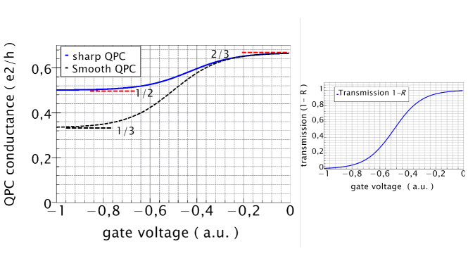
Repeating the same procedure at contacts , and and at the drain provides an efficient way to compute the conductance in presence of the QPC. Figure 5 shows the conductance variation. For comparison we have included the case of a smooth edge and smooth QPC for which the 2/3 edge separates into two reconstructed 1/3 edge channels and a plateau occurs. For full reflection, , the upper edge voltages at the QPC are while the lower edge voltages are: . The voltage drop at the QPC is . This drop could be observable using photo-assisted shot noise which presents a zero temperature noise singularity at the Josephson relation , with the microwave irradiation frequency [40, 41]. We can reproduce the same findings for energy-preserving reservoirs instead of LRs, introducing the non-equilibrium energy distribution and for EPRs around the QPC. As done for voltages in the case of LRs, we use a the generic relation:
| (28) |
where denotes some know distribution on the upstream end of a chain of EPRs and the distribution at the downstream end. Applying this relation to simplify the equations expressing the current conservation at each energy for drain, source and QPC EPRs allows to compute the conductance, which is found identical to the case of LRs.
References
- MacDonald [1990] A. H. MacDonald, Phys. Rev. Lett. 64, 220 (1990).
- Johnson and MacDonald [1991] M. D. Johnson and A. H. MacDonald, Phys. Rev. Lett. 67, 2060 (1991).
- Kane et al. [1994] C. L. Kane, M. P. A. Fisher, and J. Polchinski, Phys. Rev. Lett. 72, 4129 (1994).
- Kane and Fisher [1995] C. L. Kane and M. P. A. Fisher, Phys. Rev. B 51, 13449 (1995).
- Bid et al. [2010] A. Bid, N. Ofek, H. Inoue, M. Heiblum, C. L. Kane, V. Umansky, and D. Mahalu, Nature 466, 585 (2010).
- Takei and Rosenow [2011] S. Takei and B. Rosenow, Phys. Rev. B 84, 235316 (2011).
- Takei et al. [2015] S. Takei, B. Rosenow, and A. Stern, Phys. Rev. B 91, 241104 (2015).
- Protopopov et al. [2017] I. Protopopov, Y. Gefen, and A. Mirlin, Annals of Physics 385, 287 (2017).
- Nosiglia et al. [2018] C. Nosiglia, J. Park, B. Rosenow, and Y. Gefen, Phys. Rev. B 98, 115408 (2018).
- Park et al. [2019] J. Park, A. D. Mirlin, B. Rosenow, and Y. Gefen, Phys. Rev. B 99, 161302 (2019).
- Spånslätt et al. [2020] C. Spånslätt, J. Park, Y. Gefen, and A. D. Mirlin, Phys. Rev. B 101, 075308 (2020).
- Fujisawa and Lin [2021] T. Fujisawa and C. Lin, Phys. Rev. B 103, 165302 (2021).
- Ponomarenko and Lyanda-Geller [2023] V. Ponomarenko and Y. Lyanda-Geller, “Unusual quasiparticles and tunneling conductance in quantum point contacts in fractional quantum hall systems,” (2023), arXiv:cond-mat.mes-hall/2311.05142 .
- Manna et al. [2023] S. Manna, A. Das, and M. Goldstein, “Shot noise classification of different conductance plateaus in a quantum point contact at the edge,” (2023), arXiv:cond-mat.mes-hall/2307.05175 [cond-mat.mes-hall] .
- Meir [1994] Y. Meir, Phys. Rev. Lett. 72, 2624 (1994).
- Wang et al. [2013] J. Wang, Y. Meir, and Y. Gefen, Phys. Rev. Lett. 111, 246803 (2013).
- Gross et al. [2012] Y. Gross, M. Dolev, M. Heiblum, V. Umansky, and D. Mahalu, Phys. Rev. Lett. 108, 226801 (2012).
- Altimiras et al. [2012] C. Altimiras, H. le Sueur, U. Gennser, A. Anthore, A. Cavanna, D. Mailly, and F. Pierre, Phys. Rev. Lett. 109, 026803 (2012).
- Inoue et al. [2014] H. Inoue, A. Grivnin, Y. Ronen, M. Heiblum, V. Umansky, and D. Mahalu, Nature Communications 5, 4067 (2014).
- Banerjee et al. [2017] M. Banerjee, M. Heiblum, A. Rosenblatt, Y. Oreg, D. E. Feldman, A. Stern, and V. Umansky, Nature 545, 75 (2017).
- Rosenblatt et al. [2020] A. Rosenblatt, S. Konyzheva, F. Lafont, N. Schiller, J. Park, K. Snizhko, M. Heiblum, Y. Oreg, and V. Umansky, Phys. Rev. Lett. 125, 256803 (2020).
- Srivastav et al. [2021] S. K. Srivastav, R. Kumar, C. Spånslätt, K. Watanabe, T. Taniguchi, A. D. Mirlin, Y. Gefen, and A. Das, Phys. Rev. Lett. 126, 216803 (2021).
- Le Breton et al. [2022] G. Le Breton, R. Delagrange, Y. Hong, M. Garg, K. Watanabe, T. Taniguchi, R. Ribeiro-Palau, P. Roulleau, P. Roche, and F. D. Parmentier, Phys. Rev. Lett. 129, 116803 (2022).
- Nakamura et al. [2023] J. Nakamura, S. Liang, G. C. Gardner, and M. J. Manfra, Phys. Rev. Lett. 130, 076205 (2023).
- Hashisaka et al. [2023] M. Hashisaka, T. Ito, T. Akiho, S. Sasaki, N. Kumada, N. Shibata, and K. Muraki, Phys. Rev. X 13, 031024 (2023).
- Cohen et al. [2019] Y. Cohen, Y. Ronen, W. Yang, D. Banitt, J. Park, M. Heiblum, A. D. Mirlin, Y. Gefen, and V. Umansky, Nature Communications 10, 1920 (2019).
- Hashisaka et al. [2021] M. Hashisaka, T. Jonckheere, T. Akiho, S. Sasaki, J. Rech, T. Martin, and K. Muraki, Nature Communications 12, 2794 (2021).
- Acciai et al. [2022] M. Acciai, P. Roulleau, I. Taktak, D. C. Glattli, and J. Splettstoesser, Phys. Rev. B 105, 125415 (2022).
- de Jong and Beenakker [1996] M. de Jong and C. Beenakker, Physica A 230, 219 (1996).
- Kane and Fisher [1997] C. L. Kane and M. P. A. Fisher, Phys. Rev. B 55, 15832 (1997).
- Spånslätt et al. [2019] C. Spånslätt, J. Park, Y. Gefen, and A. D. Mirlin, Phys. Rev. Lett. 123, 137701 (2019).
- Kumar et al. [2022] R. Kumar, S. K. Srivastav, C. Spånslätt, K. Watanabe, T. Taniguchi, Y. Gefen, A. D. Mirlin, and A. Das, Nature Communications 13, 213 (2022).
- Melcer et al. [2022] R. A. Melcer, B. Dutta, C. Spånslätt, J. Park, A. D. Mirlin, and V. Umansky, Nature Communications 13, 376 (2022).
- Manna et al. [2024] S. Manna, A. Das, Y. Gefen, and M. Goldstein, “Diagnostics of anomalous conductance plateaus in abelian quantum hall regime,” (2024), arXiv:preprint [cond-mat.mes-hall] .
- Lumbroso et al. [2018] O. S. Lumbroso, L. Simine, A. Nitzan, D. Segal, and O. Tal, Nature 562, 240 (2018).
- Larocque et al. [2020] S. Larocque, E. Pinsolle, C. Lupien, and B. Reulet, Phys. Rev. Lett. 125, 106801 (2020).
- Rech et al. [2020] J. Rech, T. Jonckheere, B. Grémaud, and T. Martin, Phys. Rev. Lett. 125, 086801 (2020).
- Rebora et al. [2022] G. Rebora, J. Rech, D. Ferraro, T. Jonckheere, T. Martin, and M. Sassetti, Phys. Rev. Res. 4, 043191 (2022).
- Lin et al. [2021] C. Lin, M. Hashisaka, T. Akiho, K. Muraki, and T. Fujisawa, Phys. Rev. B 104, 125304 (2021).
- Wen [1991] X.-G. Wen, Phys. Rev. B 44, 5708 (1991).
- Kapfer et al. [2019] M. Kapfer, P. Roulleau, M. Santin, I. Farrer, D. A. Ritchie, and D. C. Glattli, Science 363, 846 (2019).
- Safi [2014] I. Safi, “Time-dependent Transport in arbitrary extended driven tunnel junctions,” (2014), arXiv:1401.5950 [cond-mat.mes-hall] .