The Pass-through of Retail Crime

Abstract

This paper shows that retailers increase prices in response to organized retail crime, revealing a substantial aspect of retail crime’s social costs. We match detailed information on store-level crimes to administrative scanner data from the universe of transactions for cannabis retailers in Washington state. Exploiting quasi-experimental variation from the timing of store-level robberies and burglaries, we find that crimes cause a 1.8% increase in retail prices at victimized stores. Nearby rivals of victimized stores increase prices by a similar amount with a two-month lag. Retailers’ price responses are not driven by demand effects, increased wholesale costs, or strategic price responses. Instead, they are consistent with precautionary security expenditures. We find the largest pass-through rates for independent stores and in less concentrated markets. We estimate that crime imposes a 1% “hidden” unit tax on affected stores, implying an annual negative welfare effect of approximately $30.6 million, with consumers bearing two-thirds of this burden.

Keywords: Retail crime, pass-through, retail pricing, market power, tax incidence
JEL Codes: L11, L81, H22, H23, K49

1 Introduction

Retail crime has surged to the forefront of public discourse in the United States, fueled by an apparent rise in organized retail crime. Retail crime imposes direct and indirect costs on businesses, individuals, and society. A comprehensive assessment of these costs is central for determining the optimal level of public crime prevention (Stigler,, 1970; Owens and Ba,, 2021). One factor often overlooked when considering the social costs of retail crime is its impact on market outcomes. In particular, crime-induced price changes, i.e., the pass-through of retail crime, have critical distributional implications and can introduce an excess burden by distorting firms’ and consumers’ decisions. Yet, evidence of a causal link between retail crime and market prices is nonexistent and the literature lacks a thorough analysis of the associated welfare effects.

We investigate the impact of organized retail crime on prices and the resulting welfare implications using the Washington state retail cannabis industry as a natural laboratory. We choose this context for three main reasons. First, similar to other retail sectors, retail crime is a common occurrence at cannabis stores and has garnered the attention of policymakers (Washington State Office of the Attorney General,, 2022). Second, rich scanner data covering the universe of upstream and downstream transactions for every cannabis store can be matched with store-level information on retail crime incidents, permitting a clean identification of the effects of retail crime on store-level outcomes and their underlying mechanisms. The detailed data further enables us to conduct a comprehensive welfare analysis using a sufficient statistics approach, drawing on insights from the tax incidence literature (Weyl and Fabinger,, 2013). Third, online sales and interstate transactions are not permitted in the Washington state cannabis industry, implying that cannabis retailers compete locally. This segregation allows us to investigate spillover effects of retail crime from victimized stores to competitors and examine the impact on aggregate market outcomes.

Exploiting quasi-experimental variation from the timing of store-level crime incidents, we use a difference-in-differences framework and compare store-level outcomes at victimized stores to outcomes in unaffected local markets. We find that victimized stores increase prices by 1.8 percent after a crime incident. The price increases remain persistent and stable nine months after an incident. In contrast, quantities sold at victimized stores return to pre-crime levels after a short but insignificant dip in the month after the crime. Similarly, we find no effect of crime incidents on wholesale costs at victimized stores. Since idiosyncratic fixed cost shocks such as property loss do not influence marginal costs, our combined results suggest that the rise in prices is consistent with increased expenditures on security or crime insurance. This is corroborated by evidence from a multitude of industry surveys, news articles and reports documenting a marked increase in crime prevention spending by retailers across diverse retail markets (U.S. Chamber of Commerce,, 2023; Dunham,, 2021; National Retail Federation,, 2022; U.S. Department of Homeland Security,, 2022).

We also investigate spillover effects from victimized stores to nearby rival stores, e.g. due to demand substitution on the part of consumers, strategic price responses, or an own-cost shock. We find that rivals of victimized stores—i.e. stores within a 5-mile radius of a victimized store—increase prices by 1.6 percent. However, in contrast to victimized stores, this price increase materializes with a two-month lag. Again, we find no effects on wholesale costs or quantities sold. The latter finding rules out demand substitution as a mechanism driving the price response at rival stores. To assess whether rivals’ price response reflects strategic complementarity in prices, we leverage the fact that—in addition to retail transactions—we observe the universe of vertical transactions between producers and retailers. This allows us to estimate the extent to which changes in stores’ own wholesale costs and the costs of their competitors are passed through to retail prices. Our results indicate that stores primarily adjust prices in response to their own costs rather than rivals’ costs. We find a marginal cost pass-through rate of 1.65, i.e. a $1 increase in a product’s wholesale price corresponds to a $1.65 increase in its retail price. The influence of rivals’ cost changes is statistically significant but economically negligible at $0.02 (from a $1 increase in wholesale price). Thus, rivals’ substantial price hikes in the wake of nearby retail crimes cannot be attributed to strategic complementarity in prices. Instead, rivals’ price effects appear consistent with an own-cost shock, e.g. due to precautionary security expenditures or higher crime insurance premiums.

The richness of our data further allows us to identify heterogeneity in price effects conditional on store and local market characteristics. First, we find that crime pass-through is higher at independent stores as compared to chains. Our findings suggest that retail crime pass-through is particularly relevant for mom-and-pop shops, while owners of multiple stores can offset costs across locations, mitigating retail crime’s impact on prices. Second, we find the largest price increases for stores operating in markets with comparably low market concentrations. This finding aligns with the idea that pass-through rates and market power are inversely related, as increased competition makes prices more sensitive to marginal costs—a theoretical prediction that relies on the curvature of firms’ cost functions (Ritz,, 2024) and on whether pass-through rates exceed unity (Miller et al.,, 2017).

Our main specification builds on the stacked difference-in-differences (DiD) estimator introduced by Cengiz et al., (2019) with treatment timing defined as the store-specific month of a crime incident. Similar to other DiD frameworks, stacked DiD estimates the causal treatment effect under the assumption of parallel trends and no anticipation. To account for biases from heterogeneous treatment effects and timing (De Chaisemartin and d’Haultfoeuille,, 2020; Goodman-Bacon,, 2021), stacked DiD creates crime incident-specific sub-experiments comparing treated stores to “clean” control stores, i.e., never-treated or not-yet-treated stores for a particular crime incident. We choose stacked DiD over related estimators (e.g., Callaway et al.,, 2024; Borusyak et al.,, 2024) because the rules for defining clean controls can be readily extended to geographic criteria. In addition to the timing-based criteria, we require incident-specific clean control stores to be located between 30 to 50 miles from the respective victimized store (which we refer to as unaffected local markets). These conditions ensure a sizeable control group that is comparable to our treatment group while at the same time minimizing confounding effects from spillovers to nearby stores (Muehlegger and Sweeney,, 2022). Our paper is one of the first to extend the stacked DiD framework to spatial criteria, contributing to the advancing literature on this methodology (Cengiz et al.,, 2019; Deshpande and Li,, 2019; Butters et al.,, 2022; Wing et al.,, 2024).

To derive the welfare implications of retail crime pass-through, we draw from the imperfect competition model by Weyl and Fabinger, (2013) which nests standard imperfect competition models, as well as the monopoly and perfect competition cases. We postulate that retail crime incidents constitute a positive marginal cost shock to affected stores that can be understood as a hidden crime tax. The implications of standard tax theory carry over to our case: i) the burden of the hidden crime tax falls disproportionately on the more inelastic side of the market; ii) under imperfect competition, there is a deadweight loss that increases with firms’ market power; iii) the pass-through rate serves as a sufficient statistic for tax incidence and the deadweight loss.

Next, we employ the framework from Weyl and Fabinger, (2013)—together with our marginal cost and retail crime pass-through estimates—to quantify the welfare effects of the crime-related price increases in the Washington state cannabis industry. At the average unit price, our estimated retail crime pass-through rate implies a $0.45 unit price increase from crime in affected markets. This unit price increase corresponds to a hidden unit tax of approximately $0.27, or about 1% of the average unit price. Given the average annual quantity sold in affected markets, our results imply an annual decrease in consumer surplus of about $20.5 million due to crime-induced price increases. In addition, we estimate a negative effect on producers of around $10.1 million, implying an incidence of the hidden crime tax on consumers of around 67% and a total social cost of retail-crime pass-through of $30.6 million. Even if we assume that the entire fictional tax revenue (the implied increase in total security expenditures at affected stores) stays within the Washington economy, our findings indicate a deadweight loss of more than $18 million from retail crime pass-through.

The implications of our findings extend well beyond the cannabis industry. Organized retail crime is common in many retail sectors and firms invest heavily in strategies to prevent retail crime (see Section 2.2). Numerous industry surveys suggest that retailers across different industries pass these costs through to consumers U.S. Department of Homeland Security, (2022); Dunham, (2021). This conjecture is supported by the findings of a study by Jackson and Tran, (2020), which reveals that increased felony larceny thresholds are associated with higher prices for automobiles and computers. The generalizability of our results is reinforced by the similarities between the retail cannabis industry and conventional retail settings in terms of cost structures and demand elasticities (Hollenbeck and Uetake,, 2021). The absence of a prevalent black market competing with legal cannabis sales further supports the broad applicability of our findings (Hollenbeck and Uetake,, 2021). A naive extrapolation of our social cost estimate, using relative sales shares and assuming retail crime impacts other retail industries similarly, suggests that the U.S.-wide social costs of retail crime pass-through exceed $120 billion. While effects are likely to be less pronounced in other sectors due to different market structures and retail crime incidence, the estimate highlights that the social costs of retail crime are significantly underappreciated when not accounting for pass-through effects.

We contribute to two broad strands of the literature. First, our study contributes to the extensive literature on the economic impact of crime and the related policy discussion on the optimal level of crime prevention. Much of this literature studies the trade off between the social costs of crime and the benefits of crime prevention (Stigler,, 1970; Owens and Ba,, 2021). We are the first to document a causal relationship between retail crime and market prices. Additionally, we provide a thorough discussion of the associated welfare implications highlighting an often neglected aspect of retail crime’s social costs.

Previous research has linked property and violent crimes to a range of economic outcomes: increased property prices (Lynch and Rasmussen,, 2001; Gibbons,, 2004; Linden and Rockoff,, 2008), economic growth (Fenizia and Saggio,, 2024), urban depopulation (Cullen and Levitt,, 1999), elevated savings levels (De Mello and Zilberman,, 2008), changes in working time (Hamermesh,, 1999), land use and crop yields (Dyer,, 2023), and even increased physical activity (Janke et al.,, 2016). More specific to our focus, several studies examine crime’s impact on consumer behavior and business dynamics. Mejia and Restrepo, (2016) highlight how crime reduces the consumption of conspicuous goods. Fe and Sanfelice, (2022) observe a crime-related decline in local food and entertainment consumption, while others identify a connection between crime and overall business activity and entrepreneurial decisions (Greenbaum and Tita,, 2004; Hipp et al.,, 2019; Rosenthal and Ross,, 2010). Using increased security expenditures as an instrument for violent crime in Columbia, Rozo, (2018) shows that increased violence leads to lower output and prices, along with a rise in firms exiting the market. Stolkin, (2023) links organized drug trafficking to higher consumer prices in Mexico, and Jackson and Tran, (2020) finds larceny thefts are positively associated with prices for computers and cars. In contrast to existing studies, we focus on organized retail crime in the U.S. and identify underlying factors behind the rise in retail prices.

Second, we contribute to the extensive literature studying the pass-through of different cost shocks, the underlying drivers, and their implications (Weyl and Fabinger,, 2013; Miravete et al.,, 2018; Miller et al.,, 2017). In our study, we examine a distinctive type of cost shock—retail crime—where costs are endogenous to firms updating their beliefs about the probability of future crime risks and outcomes. Our analysis shows that rivals’ price adjustments seem less a strategic response and more a reaction to their own increased marginal costs (e.g. due to precautionary security expenditures or increased business crime insurance premia). Such spillovers are not only relevant in the context of retail crime but also in other settings where firms compete in local markets and learning from competitors is central to firms’ costs. In these cases, price changes driven by knowledge spillovers could be mistakenly interpreted as strategic pricing.

Our heterogeneity analyses also contribute to the discussion on asymmetric strategies and market outcomes between chain and independent stores (e.g. Jia,, 2008; Hollenbeck,, 2017; Hollenbeck and Giroldo,, 2022; Janssen and Zhang,, 2023; Klopack,, 2024). We find that the pass-through of retail crime is considerably smaller for chain stores, aligning with studies that show a lack of within-chain price adjustments to local conditions (Hitsch et al.,, 2021; DellaVigna and Gentzkow,, 2019). From a welfare perspective, this pattern suggests a potential benefit to increasing the presence of chain stores within an industry. Additionally, our finding of higher pass-through rates in less concentrated markets adds to the ongoing discussion about the relationship between market competition and pass-through rates (Miller et al.,, 2017; Cabral et al.,, 2018; Genakos and Pagliero,, 2022; Ritz,, 2024).

This paper proceeds as follows. Section 2 describes the institutional context of our study, including retail crime in the United States and the retail cannabis industry. Section 3 details our data and Section 4 describes our main empirical strategy. Section 5 presents our main findings. Section 6 discusses potential endogeneity concerns and robustness checks. Section 7 outlines our policy analysis and derives the welfare implications. Section 8 concludes.

2 Institutional Background

2.1 The cannabis industry in Washington state

Approximately 50% of U.S. states have legal recreational cannabis markets. Washington state’s cannabis market opened in July 2014 for adults 21 years and older. Cannabis has since become one of the largest agricultural industries in the state, contributing $1.85 billion to gross state product (Nadreau et al.,, 2020). Cannabis consumption is widespread, with approximately 30% of Washington adults consuming cannabis on a monthly basis (Washington State Department of Health,, 2024). Consumption is relatively equal across race/ethnicity, education, and gender, but decreases monotonically with income and age. We detail the demographic characteristics of cannabis consumers in Appendix A.

The industry is regulated by the Washington State Liquor and Cannabis Board (LCB) which offers separate business licenses for upstream and downstream establishments . Producer-processors (i.e. upstream establishments) can cultivate, harvest, and process cannabis but cannot sell to end consumers. Retailers (i.e., downstream establishments) can purchase fully packaged and labeled products from producer-processors and sell them in retail stores. Producer-processors cannot own retail licenses and vice versa, creating complete vertical separation along the supply chain. Retailers can only buy from producer-processors located in Washington state and producer-processors can only sell to retailers in the state. This seals off the core of the supply chain from other U.S. states with legal recreational markets. Retailers cannot sell online, meaning retailers operate brick-and-mortar stores. Appendix A contains additional information on the cannabis supply chain.

Cannabis business licenses are capped by the LCB at 556 retailers and 1,426 producer-processors (Washington State Liquor and Cannabis Board,, 2020). Licenses are granted at the establishment level so that a single firm can own several licenses. However, a firm can only own licenses of the same type. Approximately 65% of retail stores belong to one- or two-store firms; 25% of stores belong to 3-5 store chains; less than 11% of stores belong to chains with more than 5 stores. Not all licenses are actively in business, meaning that some license holders have not opened an establishment and have no reported sales activity, especially at the producer-processor level. During our sample period, there were 508 active retailers and 692 active producer-processors.

The LCB distributes retail licenses to counties according to population density (there are no restrictions on where producer-processors can be located). Retailers are located in 37 of the 39 counties in Washington state. The average cannabis consumer in Washington is located approximately five miles from the nearest retailer (Ambrose et al.,, 2021). The geographic distribution of retail stores is illustrated in Figure 2(b), Panel (a).

Retail sales are subject to a 37% sales tax but there is no tax on upstream sales. Per month, retailers sell approximately 14,500 units and earn about $280,000 in (tax-inclusive) revenue (see Table 1(b)). However, there is substantial variation across stores, with the average monthly revenue ranging from $6,900 at the smallest store to $475,000 at the largest. For more information on the distribution of store characteristics, see Appendix A.

Table 1(b) provides an overview of the cannabis product market. Retail stores sell a variety of cannabis products—around 470 distinct products per month on average. The LCB classifies products according 12 categories (Washington State Legislature,, 2015). As Table 1(b) illustrates, usable marijuana (i.e. unprocessed dried flower) and concentrate for inhalation (e.g. for use in vape pens) account for more than 80% of all retail sales. Another 14% of retail sales comes from solid edibles (chocolate bars, gummies, etc), liquid edibles (soda and other infused drinks), and infused mix (e.g. pre-roll joints infused with concentrates). The remaining categories make up less than 2% of total revenue; these are topical products (e.g. creams and ointments), packaged marijuana mix (e.g. pre-roll joints), capsules, tinctures, transdermal patches, sample jar, and suppository.

Table 1: Product market descriptive statistics

(a) Retail store characteristics

	Monthly average per store	Sample total
Establishments		508
Units sold	15,157	263 million
	(5,829)
Distinct products	470	210,842
	(305)
Sales	$282,857	$5.07 billion
	($273,082)

Notes: Column 1 reports monthly averages at the store level. Standard deviations are in parentheses. Column 2 reports totals across all stores and months in the sample period. Sales are tax-inclusive.

(b) Retail product categories

Product category	Monthly sales (in millions of $)	Market share
Usable marijuana	$58.77	0.52
Concentrate for inhalation	$34.70	0.31
Solid edible	$8.45	0.08
Infused mix	$5.40	0.05
Liquid edible	$2.96	0.03
Other	$2.16	0.02

Notes: Column 1 reports the average monthly retail sales (in millions of dollars) across Washington state for the major product categories; Column 2 shows the corresponding market shares. Sales are tax-inclusive.

2.2 Organized retail crime

Organized retail crime in the United States

Organized retail crime is defined as large-scale theft of retail merchandise or cash, typically by two or more people, often as part of a criminal enterprise. While the exact definition varies across law enforcement agencies and jurisdictions, a defining characteristic of organized retail crime is that merchandise is not stolen for personal use but is instead resold through third-party outlets. This contrasts with petty theft (e.g. stealing baby powder because one cannot afford it), which is not the focus of our study. For ease of notation, we refer to organized retail crime and retail crime interchangeably throughout the paper.

In 2022, the U.S. Chamber of Commerce declared organized retail crime a “national crisis” (U.S. Chamber of Commerce,, 2022). According to the National Retail Security Survey (NRSS), organized retail crime is responsible for nearly $5 billion in annual losses (National Retail Federation,, 2020). Organized retail crime is pervasive in scope, with criminals targeting a variety of stores and goods (U.S. Department of Homeland Security,, 2022). Incidents are often violent in nature and threaten employee and customer safety. Many retailers invest heavily in strategies to prevent retail crime, including third-party guard services, enhanced surveillance technologies, locking cases, and employee safety and de-escalation training (see e.g. Target, (2023); Reagan and Schlesinger, (2019); Fonrouge, (2022)).

Many states have enacted legislation specifically targeting retail crime, including stiffer penalties for people caught stealing from stores with the intent to resell merchandise, and adding language targeting organized groups that rob multiple retail outlets (Lewis,, 2023). In addition to legislation, numerous local, state, and federal law enforcement agencies have created retail crime task forces across the United States (Washington State Office of the Attorney General,, 2022; U.S. Department of Homeland Security,, 2022).

Organized retail crime in cannabis

Similar to other retail sectors, retail crime is pronounced at cannabis stores. Between 2017 and 2023 there were 210 reported robberies and burglaries at cannabis retailers in Washington state. Figure 1 illustrates that retail crime in cannabis has increased over time and that the trend largely tracks data provided by the FBI on overall robberies in Washington state. This trend has prompted policymakers to take action. Retail cannabis was cited by the Washington state attorney general when creating the state’s retail crime task force (Washington State Office of the Attorney General,, 2022), and in 2023 a senate bill was introduced in the state legislature aimed at providing tax relief for security improvements at cannabis retail stores (Washington State Legislature,, 2023).

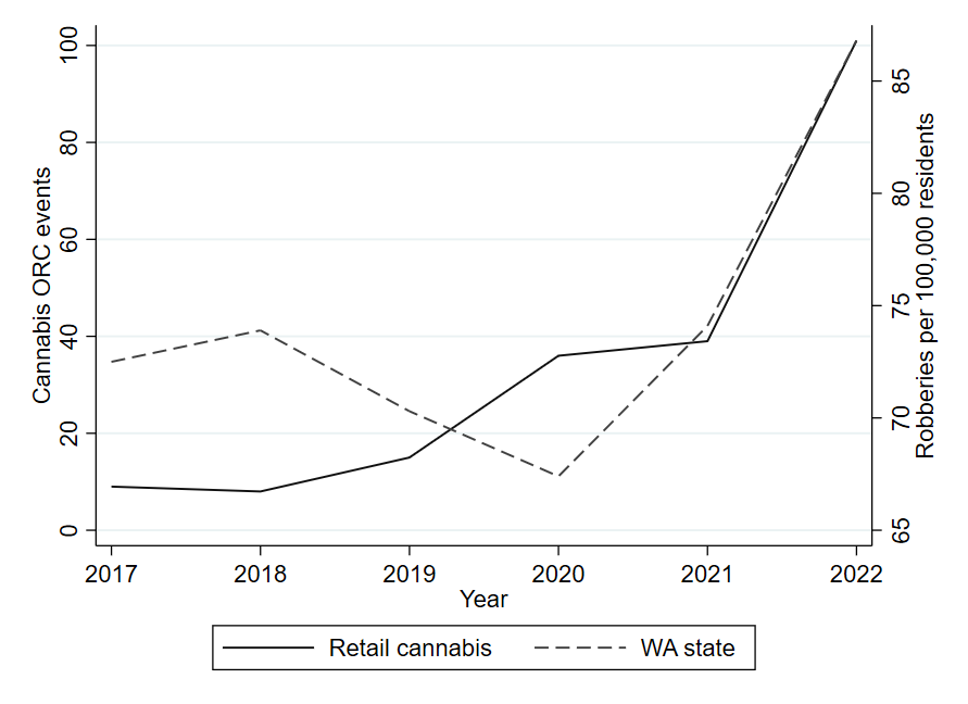
Figure 1: Comparing robberies and cannabis retail crime in Washington state

  Notes: The figure displays annually reported organized retail crime incidents in the Washington state cannabis industry (solid line) and robberies per 100,000 inhabitants in Washington state (dotted line) from 2017 to 2022. Data sources: Uncle Ike’s Robbery Tracker for cannabis industry incidents and the FBI Crime Data Explorer for state-wide robbery statistics.

Organized retail crimes in cannabis are predominantly armed robberies involving a group of perpetrators entering a store during store hours with guns drawn. Perpetrators typically extract cash from the register, demand that employees give them access to the safe, or clear shelves of merchandise. Since cannabis remains illegal at the federal level, cannabis stores do not have access to electronic payment processing services like Visa and Mastercard and nearly all retail transactions are cash-based. Stores thus handle a large amount of cash, making them prime targets for retail crime.

Robberies are often violent: in several instances, consumers or employees have been temporarily taken hostage, physically assaulted, shot at, or even killed. Victimized stores often respond to retail crime incidents by increasing security expenditures. According to the state’s Organized Retail Crime Task Force, interviews with store owners, and numerous news reports, the most common expenditure involves hiring additional security guards (Washington State Liquor and Cannabis Board,, 2022; Saldanha,, 2022; Phan,, 2022). Further preventative measures include installing panic buttons, two-way door systems, and investing in employee de-escalation training.

3 Data

3.1 Price data

To monitor developments in the cannabis market, legalization came with stringent data reporting and sharing requirements for cannabis businesses. Retailers must record all sales and regularly upload data feeds to the LCB. Compliance with data reporting is strictly enforced by the LCB. When a business is issued a violation, it can receive a fine, a temporary license suspension, or both. In cases of repeated violations, a license can be revoked by the LCB board. Given such strict enforcement, violations are uncommon. In 2022 for example, the LCB issued 63 violations among over 1,100 active licensees (Washington State Liquor and Cannabis Board,, 2024).

The data, which is reported weekly, contains detailed information on the price and quantity of each product sold by a producer-processor to a retailer, and the subsequent price and quantity of that very same product sold at the retail level. We refer to the price charged by a producer-processor as the wholesale price, and the price charged by retailers as the retail price. This reflects that producer-processors resemble wholesalers when viewed from the perspective of retailers.

The data captures granular product differentiation. To give an example, a 1.0 gram package and a 2.0 gram package of Sunset Sherbert usable marijuana (i.e. unprocessed dried flower) produced by Northwest Harvesting Co are treated as different products in the data.

The LCB switched providers for its traceability system in October 2017 and again in December 2021, creating two structural breaks in the price data. Our sample period lies between these breaks and spans March 2018 through December 2021. We obtained the data from Top Shelf Data, a data analytic firm that ingests the raw tracking data from the LCB and matches it with additional product information. The estimation sample covers the universe of sales from all 508 active retail establishments. Per month, retailers sell approximately 14,500 units and earn about $280,000 in tax-inclusive sales revenue (see Table 1(b)). Over the entire sample period, the data contain $5.07 billion in tax-inclusive retail sales. All retail prices and revenues reported in this paper are tax-inclusive.

To estimate pass-through semi-elasticities, we follow previous studies (e.g., Renkin et al.,, 2022; Leung,, 2021; Harasztosi and Lindner,, 2019) and use as our dependent variable the natural logarithm of the monthly store-level price index. The log price index measures the price inflation for store $j$ in month $t$, and is denoted as $\pi_{j,t}$:

$$\pi_{j,t}=\ln I_{j,t},\,\text{with}\,I_{j,t}=\prod_{c}I_{c,j,t}^{\omega_{c,j,y(t)}}$$ (1)

$I_{j,t}$ is an establishment-level Young price index that aggregates price changes across product subcategories $c$, where each subcategory is a unique category-unit weight combination. The index weight $\omega_{c,j,y(t)}$ is the revenue share of subcategory $c$ in establishment $j$ during the calendar year of month $t$. The dependent variable is equivalent to the first difference of the log of the weighted store price level between month $t$ and $t-1$. Store-level indices are common in the literature on retail price movements and carry several advantages over more disaggregated product-level price data. First, retail crime occurs at the store level, making the store a natural unit of analysis. Second, a store-level index allows the researcher to weigh products by their importance for each store. Finally, entry and exit occur at a much higher frequency for products compared to stores, and a product-level time series would contain frequent gaps. Since the vast majority of cannabis businesses have succeeded at staying in business, the store-level panel is much more balanced. We describe the establishment-level price index in more detail in Appendix B.

Besides prices, we are also interested in the effect of retail crime on other store-level outcomes. First, we consider the possibility that consumers substitute out of victimized and into nearby rival stores following crime incidents (e.g. due to increased prices or fear of physical harm). To investigate this, we construct a store-level quantity index measuring the monthly percent change in quantity sold. The quantity index is constructed similarly as the price index with index weights based on annual revenue shares (see Appendix B).

It is also possible that stores adjust their wholesale expenditures to offset the costs of crime. Wholesale costs are particularly important since the Cost of Goods Sold (COGS) accounts for 80% of cannabis retailers’ variable costs (see Appendix A), similar to other retail sectors (Renkin et al.,, 2022). An advantage in our setting is that we directly observe wholesale prices and quantities at the store-product-month level. We construct a wholesale cost index that captures the month over month percent change in wholesale prices paid by a store. The index weights are based on retailers’ annual wholesale expenditures (rather than annual revenue as with the price index).

Finally, we investigate whether stores adjust retail margins in response to crime. We construct a store-level margins index that measures the monthly percent change in the ratio of unit retail price to unit wholesale cost (using annual revenue weights).

Table 2 provides descriptive statistics for our indices. The price, wholesale cost, and margins indices are centered around zero and have means close to zero. Standard deviations for these indices range from 0.002 to 0.029. The quantity index has a larger variance than the other indices. This is a common characteristic of quantity indices constructed from store-level scanner data, and is similar to what is found elsewhere in the literature (see e.g. Renkin et al.,, 2022). The distributions of the indices can be found in Appendix Figure 8.

Table 2: Dependent variable descriptive statistics

	Mean	SD	Median
Log price index	-0.001	0.029	0
Log quantity index	-0.008	0.21	-0.012
Log wholesale cost index	1.18e-05	0.002	0
Log margins index	-0.001	0.029	0

Notes: This table presents the mean, standard deviation, and median of our main dependent variables: Log price index, Log quantity index, Log wholesale cost index, and Log margins index.

3.2 Retail crime data

Crime at retail cannabis stores is not formally tracked or aggregated by law enforcement agencies. However, on behalf of the market at large, Uncle Ike’s, a retailer and member of Washington’s Craft Cannabis Coalition of over 70 small businesses, maintains a public database of retail crime incidents reported by businesses, law enforcement, and the news media. While the database offers a reasonably accurate list of crimes reported to local police departments, it is not an official census of retail crime at cannabis stores. We view this as unproblematic for two reasons. First, each incident in our sample period is cross-referenced with either a police report, police case number, or a news article that references a police investigation. This makes it highly unlikely that treatment is falsely assigned to a store that is, in fact, untreated. Conversely, it is possible that not all crimes are reported to the police or news media and, hence, do not appear in the database. In that case, treated stores would potentially be misclassified as controls, leading to attenuation bias and conservative treatment effect estimates. However, since the control group is much larger than the treatment group in our setting, misclassified controls will be dominated by correctly classified controls. As a result, we expect attenuation bias from misclassified controls to be minimal.

Figure 2(b) shows the locations of stores with a reported crime during our sample period. There were 76 reported crimes at 57 different stores (46 stores were victimized only once and 12 stores were victimized more than once). Of these crimes, 62 were armed robberies and 14 were burglaries. Approximately two-thirds of these crimes occurred at stores in the Seattle area and the neighboring cities of Tacoma and Bellevue, which roughly corresponds to the share of stores in those cities compared to the rest of the state. In general, crime incidence at cannabis stores reflects the geographic distribution of stores.

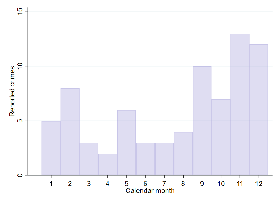
Figure 7: Reported crimes at cannabis retailers by calendar month

There is some evidence of seasonality in crime incidents at cannabis retailers, with more crimes occurring in the fourth quarter compared to other quarters (see Appendix Figure 7). Over the entire sample period, crime incidents at cannabis retailers increased, which roughly tracks the increase in reported crime in Washington state more generally (see Figure 1).

Figure 2: Retail cannabis stores in Washington state

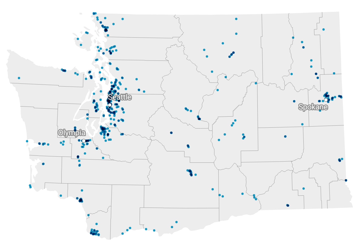
(a) Retail stores

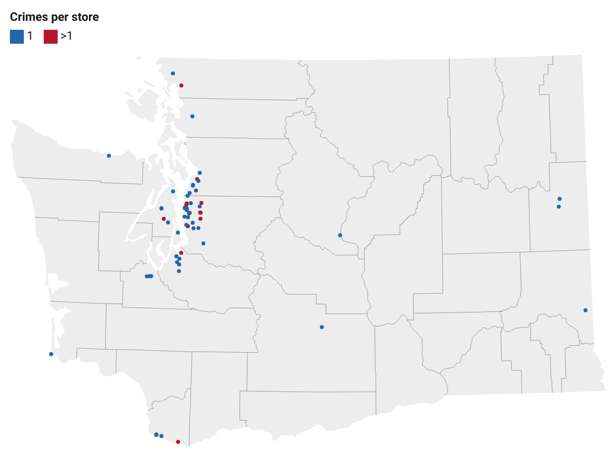
(b) Stores with reported crimes

  Notes: Panel (a) illustrates the geographical distribution of cannabis retail stores in our sample. Panel (b) shows the geographical distribution of victimized stores, with stores reporting one crime incident marked by blue dots and those with at least two reported crime incidents marked by red dots.

4 Empirical strategy

We are interested in the effect of retail crime on store-level prices. To identify a causal effect, we exploit the quasi-experimental variation in the time and location of retail crimes using a (stacked) difference-in differences (DiD) estimator. The following subsections describe our empirical strategy in more detail.

4.1 Treatment and control groups

Two treatment groups: victimized and rival stores

We define treatment timing as the store-specific month of a robbery or burglary. We distinguish between two treatment groups based on their exposure to retail crime: i) victimized stores, i.e., all stores that directly experience a robbery or burglary, and ii) rival stores, i.e., stores located within a 5-mile radius of a victimized store. The first treatment group allows us to analyze the direct impact of crime on victimized stores’ pricing strategies, while the second accounts for potential spillovers to nearby stores. Such spillovers could result from demand substitution, strategic complementarity in prices, or an own-cost shock (e.g. from precautionary security expenditures or higher business crime insurance premia). We choose the 5-mile radius for several reasons. First, victimized stores have an average of nine competing stores within this radius. This implies that a consumer at the average store can choose between several alternative stores. To the extent that crime induces changes in consumer behavior, we view it as plausible that these nearby stores may be affected. Second, the 5-mile radius is sufficiently small so as to reasonably capture local market characteristics that may influence how rival stores react to a nearby store being victimized. Results are robust to adjusting the boundary (see Appendix F). In assigning treatment to a larger group of nearby units, our strategy resembles those from the spatial treatment literature (see e.g. Keiser and Shapiro,, 2019; Lipscomb and Mobarak,, 2017).

Control group: unaffected local markets

We compare both treatment groups to a common control group: stores in unaffected local markets. In defining unaffected local markets, we face a tradeoff. On the one hand, we want to ensure that stores in the control group are in markets that are comparable to (and hence near) the treated group. At the same time, if there are spillovers from the treated group to nearby stores, then including nearby stores in the control group leads to biased estimates. In this subsection, we identify potential spillovers and use them to guide our definition of unaffected local markets.

One concern is strategic complementarity in pricing. Muehlegger and Sweeney, (2022) show that in the presence of imperfect competition, the strategic response of (untreated) competitors may disqualify them as a valid control group. In practice, this implies that the price a firm sets is a function of not just its own costs, but also those of its rivals. A major advantage in our setting is that—in addition to retail prices and quantities—we also observe prices and quantities for the universe of vertical transactions between producer-processors and retailers. This allows us to measure retailers’ spatial sensitivity to competitors’ costs and identify the distance at which retailers no longer compete in prices. In Appendix D, we estimate the pass-through of the average wholesale costs of competing stores within a certain distance from store $j$ on store $j$’s retail prices. We find that sensitivity to competitors’ unit costs dissipates by the 30-mile mark under a variety of specifications (see Appendix D for more details). This suggests that stores located more than 30 miles from a victimized store will not have a strategic price response to the victimized store’s crime pass-through, and hence serve as valid controls from a strategic pricing standpoint.

Spillovers can also arise if consumers substitute demand out of victimized stores and into nearby competitors, e.g. out of fear for their own safety or temporary crime-induced store closures. While demand substitution is distinct from strategic complementarity in pricing, at a mechanical level both entail consumers choosing between stores from the same choice set. Therefore, we view the 30-mile boundary for strategic pricing as a plausible boundary for demand substitution as well.

Finally, spillovers can occur if crime incidents induce a cost shock at rival stores. There are at least two potential reasons for such a cost shock. First, upon learning about crime at a victimized store, rival stores may update their own expectations of being victimized and invest in precautionary security measures. While the geographic scope of such knowledge spillovers and precautionary expenditures is difficult to measure, it is plausible that stores located close to a victimized store are more likely to update their expectations of being victimized compared to stores located further away, e.g. due to local market characteristics. Therefore, we expect this channel to operate within a similar geographic radius as strategic complementarity in pricing and demand substitution. Second, if crime incidents cause insurers to reevaluate the crime risk in local markets, then retailers may face higher crime insurance premia. Since crime insurance premia are typically a function of the number of employees at a store as well as store revenues and size, a hike in premia may amount to a marginal cost shock.

While potential spillovers require omitting nearby stores from the control group, it is important to ensure that the control group remains comparable to the treated stores to the greatest possible extent. We therefore limit the distance at which a store can serve as a control to 50 miles. Unaffected local markets thus consist of stores located in the concentric “donut” between 30 and 50 miles from a victimized store. We conduct several robustness checks to test the sensitivity of our main results to adjusting the boundaries for unaffected local markets (see Appendix F).

Panel (a) in Table 3 compares pre-treatment characteristics of treated and untreated stores in our study. Columns 1 and 2 show that the average unit price at victimized and rival stores is similar prior to treatment. Victimized stores sell more products per month, have higher monthly revenue, and have more product variety compared to rival stores, though the differences are small and never statistically significant. The similarities between victimized and rival stores prior to crimes support our assertion that the location of crime incidents is conditionally quasi-random. Column 3 summarizes the never-treated group and is based on the entire sample period. Note that never-treated stores may or may not serve as controls depending on their location. The mean price at never-treated stores is similar to victimized and rival stores, but the quantity sold, monthly revenue, and product variety are lower than at victimized and rival stores. This could reflect that victimized and rival stores are primarily located in densely populated urban areas, whereas never-treated stores may contain a larger share of rural stores. Our definition of unaffected local markets effectively controls for such differences. Panel (b) of Table 3 shows the number of stores in each group (victimized, rivals, and never-treated).

Table 3: Estimation sample summary statistics

(a) Pre-treatment characteristics
	(1)	(2)	(3)
	Victimized	Rivals	Never-treated
Unit price (in dollars)	26.24	25.47	26.00
	(4.33)	(4.49)	(4.50)
Units sold per month	13,260	12,304	10,908
	(12,409)	(11,931)	(11,617)
Monthly revenue (in dollars)	248,516	215,201	210,416
	(234,911)	(217,957)	(235,890)
Unique products per month	505	425	393
	(388)	(346)	(324)
(b) Treatment group sizes
Stores	57	264	137
Control stores	329	321
Total store-months	15,949	17,055

Notes: Panel (a) summarizes store-level variables prior to treatment, with statistics for the never-treated group based on the entire sample period. Standard deviations are in parentheses. The reported variables include unit price, average store quantity sold per month, average store revenue per month, and average number of distinct products sold per month. Columns 1-2 display summary statistics for the two treatment groups: victimized stores and rival stores. Column 3 presents data for stores that are never in one of the treatment groups and may or may not serve as controls depending on their location. Panel (b) shows the number of stores in each treatment group.

4.2 Main specification

Our main specification builds on the stacked DiD estimator. Stacked DiD has been applied in a variety of settings, including investigating the effect of local cost shocks on national retail chains (Butters et al.,, 2022), the effect of application costs on the targeting of disability programs (Deshpande and Li,, 2019), and the effects of minimum wage hikes on low wage employment (Cengiz et al.,, 2019). Stacked DiD overcomes issues with canonical DiD which can yield biased estimates under staggered treatment adoption and heterogeneous treatment effects (see, e.g., Baker et al., (2022); Goodman-Bacon, (2021); Sun and Abraham, (2021); Callaway and Sant’Anna, (2021)). Similar to other DiD estimators, the stacked DiD estimator identifies the causal treatment effect under the assumption of parallel trends and no anticipation. We discuss these identifying assumptions and other threats to identification in more detail in Section 6.

The idea behind stacked DiD is to create a separate dataset (i.e. sub-experiment) for each crime incident comparing the treated group for that incident to a set of “clean” controls. An identifying variable is generated for each dataset and the datasets are concatenated to create a single “stacked” dataset. The model is estimated on the stacked data with sub-experiment-specific unit- and time-fixed effects.

Most studies using stacked DiD define clean controls solely based on treatment timing as this accounts for biases from heterogeneous treatment effects under staggered adoption. We add a geographic layer to the clean control criteria to remove additional contamination from treatment effect spillovers. Thus, to be considered a clean control for a given sub-experiment, a store must be (i) a never-treated or not-yet-treated store outside of its own event window, (ii) located between 30-50 miles of the corresponding crime incident, and (iii) cannot be within 30 miles of a victimized store whose event window overlaps with the focal incident.

The flexibility of the stacked DiD estimator in extending rules for clean controls to geographic criteria is crucial in our setting. In particular, stacked DiD reduces biases from spillovers to untreated stores, maintains geographically comparable treatment and control stores, and ensures a large pool of clean control stores. This feature is the primary reason we choose the stacked DiD estimator over related estimators (Callaway and Sant’Anna,, 2021; Borusyak et al.,, 2024) which typically impose restrictions on the control group composition for the entire sample and thereby significantly reduce the pool of valid control observations. Details about our inclusion criteria for clean controls and the advantages of using stacked DiD compared to other estimators are discussed in Appendix E.

For each sub-experiment, stacked DiD identifies a group average treatment effect for the treated (ATT), similar to the cohort-specific ATT in Sun and Abraham, (2021) and the group-time ATT in Callaway et al., (2024). Moreover, when there is balance in the number of pre-and post- treatment periods across sub-experiments, the stacked DiD regression recovers an aggregate ATT that is a convex combination of underlying causal effects (Wing et al.,, 2024). Since our setting contains several crime incidents near the beginning and end of the sample period, dropping these incidents substantially reduces our treatment sample size. Therefore, in our main specification we allow for compositional imbalance in pre- and post-treatment periods across sub-experiments. Nevertheless, we impose compositional balance in a robustness check and find very similar results (see Section 6).

For estimation, we specify a distributed lag model with leads and lags before and after treatment adoption. We define treatment adoption, $\Delta T_{j,d,t-l}$, as a dummy variable that is equal to one if store $j$ is treated $l$ months after period $t$ (or $l$ months before when $l$ is negative), and equal to zero otherwise. In our main specification, we drop stores with multiple treatments from the sample prior to the second treatment so as to isolate the effect of the first crime on store prices (we allow for multiple treatments in a robustness check in Section 6). Since the store-level price indexes and the treatment adoption indicators are in first-differences, we estimate the following model in first-differences:

$$\pi_{j,t,d}=\sum_{l=-k+1}^{k}\beta_{l}\Delta T_{j,d,t-l}+\gamma_{t,d}+\epsilon_{j,d,t}$$ (2)

Equation 2 relates the monthly inflation rate at store $j$, $\pi_{j,t,d}$, to leads and lags of the treatment adoption indicator, $\Delta T_{j,d,t-l}$, for store $j$ in sub-experiment $d$. We control for sub-experiment-by-time fixed effects, $\gamma_{t,d}$. Since the model is in first differences, store FE are swept out. Since the identifying variation is at the store level, standard errors are clustered by store to allow for autocorrelation in unobservables within stores, similar to Butters et al., (2022); Deshpande and Li, (2019).

The parameter $\beta_{l}$ measures the change in establishment $j$’s inflation resulting from a robbery or burglary $l$ months after a crime (or $l$ months before when $l$ is negative) compared to the control group. While inflation is the dependent variable, we follow previous studies and present the estimates as the effect of treatment on the price level (see e.g. Renkin et al., (2022); Leung, (2021)). We thus normalize the effect on the price level to zero in the baseline period one month before treatment and report the cumulative treatment effect as the sum of $\beta_{l}$ at various lags: $E_{L}=\sum_{l=0}^{L}\beta_{l}$. The pre-treatment coefficients are reported in a similar manner with $P_{-L}=-\sum_{l=-1}^{-L+1}\beta_{l}$. This linear transformation is commonly applied in studies with a dependent variable that is in first-differences (Renkin et al.,, 2022; Leung,, 2021). The cumulative distributed lag coefficients are numerically equivalent to the parameter estimates from an event study design under constant treatment effects outside the effect window (Schmidheiny and Siegloch,, 2023).

An important consideration is the number of leads and lags to include in equation 2. One limitation is that the establishment panel is not balanced, meaning that changes in the underlying sample may affect estimates when $l$ is large. Therefore, in our baseline estimation, we set $k=5$. This implicitly assumes constant treatment effects outside of the 11-month event window, i.e. $\beta_{l}=0\;\forall\;l>|k|$. We show in Appendix F that treatment effects remain stable over a longer event window.

Our main analysis investigates the effects of retail crime on prices at retail cannabis stores. However, we are also interested in the effects of retail crime on other store-level outcomes, as this sheds light on the underlying factors driving retail crime pass-through. For this purpose, we estimate equation 2 using the store-level quantity indexes, wholesale cost indexes and retail margin indexes as dependent variables (we describe these variables in detail in Section 3).

5 Results

5.1 Main results

Figure 3(a) shows the estimated price level effects for victimized and rival stores according to our main specification. We report cumulative effects, i.e. the effect on the price level (in percent) relative to the baseline period in $t-1$ (see Section 4 for details). For both groups, the figure shows no significant pre-treatment effects. In the month of a retail crime incident, however, prices at victimized stores increase and continue to rise for three months. Four months after the crime, prices at victimized stores are 1.8% higher compared to the month before the crime and stay at this higher price level for the following months. In contrast, rival stores show no price increase in the month that a retail crime hits a nearby store. Nevertheless, two months after crime incidents at victimized stores, a very similar price increase can be observed at rival stores. Four months after the crime, rival store prices are 1.6% higher than the month before the crime, and the effect is not statistically significantly different from that at victimized stores. Overall, our estimates reveal that retailers in the Washington state cannabis market increase their prices following retail crime incidents.

Figure 3: Effect of crime on store outcomes

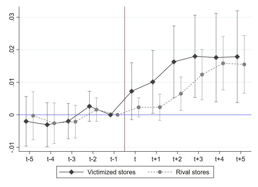
(a) Price level

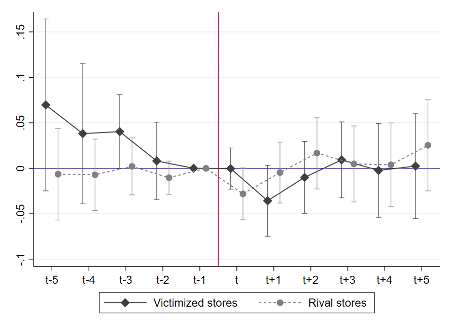
(b) Quantity sold

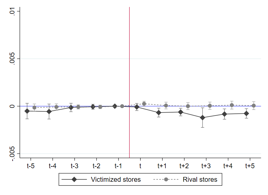
(c) Wholesale cost

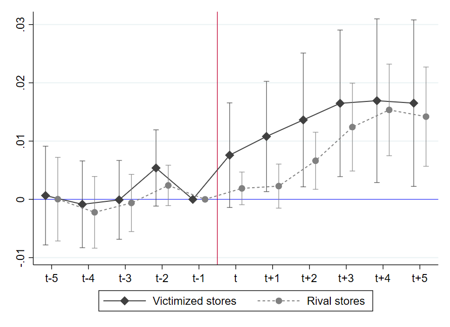
(d) Retail margins

  Notes: Each panel shows the cumulative treatment effects ($E_{L}$) $L$ months after a crime on different outcomes, along with corresponding 90% confidence intervals based on standard errors clustered at the store level. Coefficients are interpretable as percent increases in outcome levels relative to the month before a crime incident. The black line depicts the cumulative effects of crime on outcomes at victimized stores, while the grey line represents rival stores. The dependent variables are: store-level price index (Panel (a)), store-level quantity index (Panel (b)), store-level wholesale cost index (Panel (c)), and store-level margins index (Panel (d)).

Figure 3(b) presents estimates from equation 2 when using the quantity index as the dependent variable. Pre-incident estimates are insignificant at the 10% level for both store types. Our findings indicate a 3% (but insignificant) decrease in quantity sold for both victimized and rival stores immediately after a crime incident. However, the quantity sold returns to pre-incident levels within a month. This finding speaks against demand substitution out of victimized and into rival stores due to, e.g., stigmatization or personal safety concerns on the part of consumers. Moreover, our findings suggest that demand in our setting is relatively inelastic. This is consistent with high search costs and aligns with previous evidence from Hollenbeck and Uetake, (2021). Finally, the results indicate that our estimated price effects are not confounded by underlying changes in demand.

Figure 3(c) shows estimates with the wholesale cost index as the dependent variable. Estimated monthly treatment effects on wholesale costs are statistically significant but economically small, at approximately 0.1%. These negligible effect sizes imply that retailers do not meaningfully adjust their wholesale expenditures in response to retail crime incidents, and also indicate no major reaction from wholesalers to the crime incidents at their client stores. Additionally, these results provide reassurance that changes in COGS are not a confounder driving the observed retail price effects in Figure 3(a). Pre-incident effects show no discernible divergence in the evolution of wholesale costs between the treatment and control groups.

Lastly, we explore the impact of retail crime on retail margins, which serve as a proxy for retailers’ profits. Given the absence of effects on wholesale costs, the treatment effects on retail margins expectedly reflect the estimated price effects, as shown in Figure 3(d). Unfortunately, we do not observe detailed profit data for retailers, which could provide further insights into other factors driving the price effects.

5.2 Heterogeneity analysis

In this subsection, we conduct two main heterogeneity analyses to gain more insight into the role of market structure in crime pass-through.

Chain vs Independent stores

We first examine whether crime pass-through differs between chain and independent stores. One concern is that chain size may correlate with profitability and is therefore endogenous. This is less of a concern in our setting for two reasons. First, when the market was initially created, the LCB randomly assigned licenses to applicants, reducing self-selection bias for store types Hollenbeck and Giroldo, (2022). Second, the number of licenses is capped by the LCB, meaning that profitable firms cannot easily increase their chain size.

We define chains as stores belonging to firms running three or more stores and consider all other stores as independent. Of the 508 stores in our sample, 330 are independent and 181 belong to a chain. We split our sample into two subgroups according to this definition and estimate our main specification separately for each subgroup. Table 4 reports the results of the subsample analyses. Columns 1 and 2 show that among victimized stores, the pass-through of crime is large at independent stores but small and not statistically significantly different from zero at chain stores. Columns 5 and 6 show that the same pattern holds among rival stores. Results are similar when defining independent as single-store firms and chains as firms with two or more stores (see Appendix Table 11). Our findings align with studies showing little within-chain price adjustments to local conditions (Hitsch et al.,, 2021; DellaVigna and Gentzkow,, 2019) and suggest that owning multiple stores may serve as insurance against negative cost shocks, possibly due to better financing conditions or high returns to scale (Hollenbeck and Giroldo,, 2022). Alternatively, or as an additional mechanism, the results suggest that chains may already have more effective crime prevention strategies or insurance plans in place that require less adjustment, supporting the notion of firm learning.

Market concentration

Next, we investigate whether effects vary by market concentration. Concentration is endogeneous if profitability affects market entry. However, since the LCB caps the number of cannabis store licenses and distributes them according to population density, profitability does not directly affect concentration in our setting. We consider each store in our sample (including non-treated stores) as the focal point of its own market comprising the set of stores (including the focal store) within a 5-mile radius. We calculate the Herfindahl–Hirschman Index (HHI) for each market in the sample, and we then divide the sample into two subgroups for stores above and below the sample median HHI. A high HHI implies high concentration and thus low market competition. We provide descriptive statistics on the HHI in Table 9.

We estimate our main specification on each subsample to test whether crime pass-through differs between stores above and below the median HHI. We report results in Table 4. Columns 3 and 4 show that among victimized stores, crime causes prices to increase 3.1% in low-concentration markets while in high-concentration markets the effect is not significantly different from zero. Moreover, the difference in effect sizes is statistically significant. This pattern carries over to rival stores, though the difference in effects sizes between low and high market concentration is less pronounced. Prices in low-concentration markets increase 2.2% while in high-concentration markets they increase 1.1%.

The heterogeneous pass-through rates may be attributable to differences in rural and urban markets. The LCB awards licenses to counties according to population density, and market concentration likely decreases with population density. Since wages are higher in more populated areas, and crime may induce a labor cost shock, it is plausible that crime induces a larger cost shock at stores in densely populated urban areas. In a robustness check, we find that once rural-urban differences in market concentration are accounted for, the difference in effect size between low- and high-concentrated markets becomes slightly smaller but largely persists (see Appendix Table 11). We explore this issue in more detail in Appendix C.

These results are in line with standard imperfect competition models (e.g. the canonical Cournot model) which predict that when competition increases, prices become more sensitive to marginal costs and pass-through rates rise. However, if marginal cost pass-through rates exceed unity, predictions regarding the relationship between competition and pass-through rates can change (Weyl and Fabinger,, 2013; Miller et al.,, 2017). This is an important consideration in our context, as we find marginal cost pass-through rates greater than one in Section 7. Moreover, Ritz, (2024) show that the positive relationship between competition and pass-through rates is sensitive to the shape of the cost function. Empirical findings on the relationship between competition and cost pass-through rates are similarly mixed. Some studies report that pass-through rates increase with competition (Cabral et al.,, 2018; Genakos and Pagliero,, 2022), while other studies find the opposite (Doyle Jr and Samphantharak,, 2008; Miller et al.,, 2017).

Table 4: Heterogeneity

	Victimized				Rivals
	(1)	(2)	(3)	(4)	(5)	(6)	(7)	(8)
	Indep. stores	Chain stores	Low concentration	High concentration	Indep. stores	Chain stores	Low concentration	High concentration
$E_{0}$	0.010	0.0014	0.012	0.0019	0.0025	0.0033	0.0019	0.0038
	(0.0078)	(0.0027)	(0.0097)	(0.0027)	(0.0022)	(0.0029)	(0.0026)	(0.0023)
$E_{2}$	0.021**	0.0063	0.024**	0.0075	0.010***	0.00062	0.0077	0.0062*
	(0.0096)	(0.0050)	(0.011)	(0.0060)	(0.0037)	(0.0048)	(0.0049)	(0.0033)
$E_{4}$	0.024**	0.0035	0.031**	0.0011	0.024***	0.0042	0.022***	0.011*
	(0.012)	(0.0056)	(0.013)	(0.0088)	(0.0060)	(0.0076)	(0.0073)	(0.0063)
$\sum\text{Pre-event}$	-0.0016	-0.0013	0.0015	-0.0059	-0.0030	-0.00014	0.00049	-0.0053
	(0.0063)	(0.0055)	(0.0063)	(0.0067)	(0.0050)	(0.0075)	(0.0073)	(0.0058)
$N$	15,355	14,929	15,197	15,087	13,863	11,657	13,231	12,289

Notes: Each column shows the cumulative treatment effects on store price levels for different subsamples zero, two, and four months after a crime, along with the sums of pre-treatment coefficients. Coefficients are interpretable as percent increases in outcome levels relative to the month before a crime incident. The first four columns use victimized stores as the treatment group, and the last four columns consider rival stores. Columns 1 and 5 show effects for independent stores (i.e., owned by firms running one or two stores only), while columns 2 and 6 show effects for stores owned by firms running at least three stores. For the other columns, the Herfindahl-Hirschman Index is calculated for the market around each store (including non-treated stores) within a 5-mile radius, and the sample is split according to the median market concentration across all markets. Columns 3 and 7 show effects for treated stores in markets with below median concentration, and columns 4 and 8 for treated stores in markets with above median concentration. Standard errors of the sums are clustered at the store level and shown in parentheses. ^∗ $p<0.10$, ^∗∗ $p<0.05$, ^∗∗∗ $p<0.01$.

6 Threats to identification, robustness checks and alternative specifications

In this section, we address potential endogeneity concerns in our setting. We present various alternative specifications, robustness checks and placebo tests to corroborate the validity of our results.

Endogenous treatment timing and parallel trends

The key identifying assumption of our empirical strategy is the parallel trends assumption. This implies that store-level prices in the control and treatment groups would have followed a common trend in the absence of retail crime incidents.

In our framework, we account for all time-invariant factors that could influence treatment, such as store location and average revenues, through the inclusion of store-fixed effects. Similarly, we account for all time-varying factors that equally apply to all stores, such as the seasonality of robberies or COVID-19 effects, through the month-year fixed effects. However, the parallel trends assumption can be violated if the timing and location of retail crimes are correlated with changes in our outcome variables. An example is if stores that strongly increase or decrease revenues are more likely to be robbed or burglarized. This is less of a concern with rival stores’ treatment timing. However, it is also possible that changes in policing in certain areas are correlated with revenues in those areas, which could also threaten the causality for our rival store regression.

The first clear indication of the validity of the parallel trends assumption in our setting is the lack of significant pre-trends across all main specifications. Figure 3 shows no pre-treatment differences for prices, quantity sold and wholesale cost between victimized, rival, and control stores. Furthermore, pre-trends remain insignificant for alternative specifications, for instance, if we expand the event window (Figure 12) or when using alternative estimators (Appendix E.1). Additionally, the lack of observable pre-trends supports the validity of the second identifying assumption regarding no anticipation. If store owners anticipate robberies, we would expect to see changes in the outcome variables before the actual events.

To further corroborate our findings, we conduct placebo tests, in which we run our main regression analysis with the actual treatment timing shifted by 12 months in both directions. This approach tests for the presence of non-parallel trends or seasonal variations not fully addressed by our fixed effects. The placebo test results, detailed in Appendix Table F.14, reveal no discernible patterns, reinforcing our confidence in the validity of the parallel trends assumption and our empirical model.

Alternative estimators

The stacked DiD estimator offers advantages over related estimators due to its flexibility for applying rules for clean controls based on geographic criteria (for more details, see Appendix E). Nevertheless, other estimators may have advantages in terms of efficiency and comparability to other studies. To assess whether our findings are sensitive to the choice of estimator, we estimate dynamic treatment effects using three alternative estimators: i) the canonical two-way fixed effect DiD estimator ii) the imputation estimator developed by Borusyak et al., (2024) (BSJ); and iii) the estimator proposed by Callaway and Sant’Anna, (2021) (CS). Following our main approach, we first estimate a distributed lag model (Equation 2) for the designated event window and then calculate cumulative treatment effects using the last pre-treatment period as our baseline. We discuss the details of the alternative estimators in Appendix E.1.

The dataset used for alternative estimators includes all stores, which means the control group may comprise stores within 30 miles of victimized stores. Positive price effects at these nearby stores, as suggested by our main results, would thus imply that treatment effects are attenuated in these models. Restricting the sample to stores more than 30 miles away from any treated stores reduces the number of (potential) control stores from 329 to just 78 stores, highlighting the benefits of using the stacked DiD framework in our setting.

Table 13 displays the cumulative treatment effects at $k=0$, $k=2$, and $k=4$ for the alternative estimators. As expected, the effects are slightly smaller than in our main specification—about 1.5% for victimized stores and 1% for rival stores, except for the CS specification, which yields higher effects for victimized stores. However, in the majority of these alternative specifications, treatment effects are statistically significant and not different from our main specification, demonstrating that our findings are not driven by the choice of our estimator.

Alternative definitions of unaffected local markets and rival stores

When defining clean control stores, we balance comparability with treated stores against potential biases from treatment spillovers, as discussed in Section 4. To investigate whether our estimated effects are sensitive to our definition of clean control stores, we estimate our model using alternative definitions of unaffected local markets and rival stores.

First, we expand the area of unaffected local markets along two dimensions: i) including all stores within 10 and 50 miles of victimized stores; ii) including all stores that are located more than 30 miles away from victimized stores. Figures 13(a) and 13(b) in Appendix F show that, as anticipated under positive spillover effects, treatment effects fall slightly to around 1.6% (victimized) and 1.3% (rivals) when expanding the inner boundary, but remain statistically significant. A similar picture emerges if we include more distant stores in the control group, as treatment effects slightly decrease but remain statistically significant.

Next, we inspect the sensitivity of our results to expanding the inner ring that defines rival stores. We report results in Figure 13(c) in Appendix F. Interestingly, the treatment effect remains roughly constant when we include all stores within a 10-mile radius as rivals, and only declines for stores located further away. These results suggest that spillover effects may apply to a larger set of stores than initially thought. Furthermore, the declining treatment effect beyond the 10-mile radius indicates that spillovers decrease with distance from the crime incident. This provides supportive evidence for our choice of control stores, as it suggests that stores located further away from victimized stores are less likely to be contaminated by spillovers.

Additional Robustness checks

We conduct a number of additional robustness checks to rule out other factors potentially driving our findings. We present the results of these robustness checks in Table 5. In both panels, Column 1 reproduces our baseline specification from Figure 3(a). Column 2 shows that our results are similar when we include control variables such as county population, the local house price index (at the three-digit zip code level), and average county wage. These control variables absorb variation in prices stemming from local business cycles, population growth, or fluctuations in the housing market (Stroebel and Vavra,, 2019).

Since our price indexes are store-level aggregations of diverse sets of products and product categories, it is important to check whether results hold for a narrower set of homogeneous products. Therefore, in Column 3 we restrict the sample to products belonging to the usable marijuana product category and convert all prices to price per gram. Effect sizes are larger using this price index, though we show in Appendix 5.2 that this is due to larger effects for usable marijuana compared to other product categories. In Column 4 we winsorize inflation rates below the bottom 0.5 percentile and above the 99.5 percentile to show that our results are not driven by outliers.

Our price indexes are constructed with weights based on calendar year revenue shares (see Section 3). To ensure that our main effects are not an artifact of this weighting scheme, in Column 5 we use indexes constructed with weights based on the fiscal year running from July through June. Estimates are similar to our baseline specification, though for victimized stores the standard errors are larger at higher lags.

Our main analysis only includes a store’s first reported crime incident and hence does not capture the effects of subsequent crimes at stores that are victimized more than once (of the 57 victimized stores in our sample period, 12 stores have multiple crime incidents). In Column 6, we include all reported crimes which allows for individual stores to be treated more than once. For victimized stores, treatment effects are slightly higher shortly after crime incidents but become attenuated at later lags when allowing for multiple treatments. This is in line with the idea that store owners invest more following the first event but react less to subsequent events. This finding is reaffirmed when looking separately at treatment effects from subsequent crime incidents only (see Appendix Figure 9(b)). One month after a subsequent crime incident, prices show a slightly higher treatment effect than for the first crime, but price levels quickly return back to the level before the subsequent crime event. Note, however, that estimates, particularly at the end of the event window, become very noisy given the limited number of observations.

Allowing multiple treatments also attenuates price effects at rival stores (Panel (b) Column 6). Similarly, when looking separately at subsequent incidents we find a small effect of subsequent crimes on rival store prices (see Appendix Figure 9(b)).

By excluding recently or soon-to-be-treated stores from the control group, stacked DiD identifies an incident-specific ATT for each crime incident under the standard DiD assumptions of parallel trends and no anticipation. Wing et al., (2024) show that even when the DiD assumptions hold within each sub-experiment, the aggregated parameter estimate can be biased if the stacked dataset is not balanced in the number of pre- and post-periods across sub-experiments. This is the case if some crime incidents occur near the beginning or end of the period for which data are available so that causal effects are identified for a larger number of event-time periods for some crime incidents than others. The bias arises because changes in the aggregate parameter may reflect compositional changes rather than treatment effect dynamics. To account for this, in Column 7 we estimate our stacked DiD regression using the subset of crime incidents for which the entire event window falls within our sample period. In both panels of Table 5, Column 7 shows that imposing compositional balance in pre- and post-treatment periods substantially reduces our sample size but does not meaningfully change our estimates. Standard errors tend to be larger due to the reduced sample size, but the effects are still significant at the 10% level.

Stacked DiD implicitly weights treatment and control trends differently across sub-experiments. This can lead to bias in the aggregate parameter estimate if the share of treated and control stores differs across sub-experiments. The bias can arise even if the incident-specific ATTs are unbiased and there is compositional balance in pre- and post-periods across sub-experiments. Wing et al., (2024) show that this bias can be corrected by using sample weights that account for relative treatment and control group shares. Using the balanced stacked dataset (from Column 7), we estimate a weighted least squares regression using sample weights based on relative treatment shares in each sub-experiment. We report results in column 8 of Table 5. Effect sizes are slightly lower but not statistically significantly different from our baseline estimates. The estimates are significant at the 10% level.

Table 5: Price effects at victimized and rival stores - robustness checks

(a) Victimized stores
	(1)	(2)	(3)	(4)	(5)	(6)	(7)	(8)
	Baseline	Controls	Price per gram	Wins.	Alt. weights	Mult. treatments	Bal-anced (unweighted)	Bal-anced (weighted)
$E_{0}$	0.008	0.008	0.009	0.008	0.007	0.016*	0.009	0.009
	(0.006)	(0.006)	(0.007)	(0.006)	(0.005)	(0.009)	(0.009)	(0.009)
$E_{2}$	0.016**	0.016**	0.024***	0.016**	0.013*	0.022**	0.019*	0.019*
	(0.007)	(0.007)	(0.009)	(0.007)	(0.008)	(0.009)	(0.010)	(0.010)
$E_{4}$	0.018*	0.017*	0.026**	0.018*	0.015	0.015**	0.019*	0.019*
	(0.009)	(0.009)	(0.011)	(0.009)	(0.010)	(0.007)	(0.011)	(0.011)
$\sum\text{Pre-event}$	-0.001	-0.000	-0.004	-0.002	0.001	0.009	-0.002	-0.002
	(0.005)	(0.005)	(0.008)	(0.005)	(0.004)	(0.010)	(0.007)	(0.007)
$N$	15,294	15,294	15,258	15,294	15,294	17,294	11,182	11,182
(b) Rival stores
	(1)	(2)	(3)	(4)	(5)	(6)	(7)	(8)
	Baseline	Controls	Price per gram	Wins.	Alt. weights	Mult. treatments	Bal-anced (unweighted)	Bal-anced (weighted)
$E_{0}$	0.002	0.002	0.003	0.001	0.003	0.000	0.001	-0.0003
	(0.002)	(0.002)	(0.004)	(0.002)	(0.002)	(0.001)	(0.003)	(0.003)
$E_{2}$	0.005	0.005	0.008	0.005	0.004	0.002	0.002	0.002
	(0.003)	(0.004)	(0.005)	(0.003)	(0.003)	(0.002)	(0.004)	(0.004)
$E_{4}$	0.017***	0.016***	0.020***	0.014***	0.014**	0.005*	0.012*	0.011*
	(0.006)	(0.006)	(0.007)	(0.005)	(0.006)	(0.002)	(0.006)	(0.006)
$\sum\text{Pre-event}$	-0.002	-0.001	-0.005	-0.001	0.001	-0.003*	-0.007	-0.008
	(0.005)	(0.005)	(0.006)	(0.005)	(0.004)	(0.002)	(0.006)	(0.006)
$N$	16,142	16,142	16,084	16,142	16,142	21,898	12,406	10,579

Notes: Each column shows the cumulative treatment effects on store price levels for different specifications zero, two, and four months after a crime, along with the sums of pre-treatment coefficients. Coefficients are interpretable as percent increases in outcome levels relative to the month before a crime incident. Panel A uses victimized stores as the treatment group, and Panel B considers rival stores. Column 1 in each panel shows the cumulative treatment effects from the main specification. Column 2 includes additional time-varying control variables: county population, local house price index (at the three-digit zip code level), and average county wage. Column 3 restricts the sample to Usable Marijuana products and converts all prices to price per gram. Column 4 uses store-level price indexes winsorized at the 0.5 and 99.5 percentiles as the dependent variable. Column 5 uses price indexes weighted based on the fiscal year running from July through June as the dependent variable. Column 6 considers subsequent store-level crimes as additional treatment events. Column 7 shows effects for events with a completely observable and balanced event window. Column 8 applies the sample weights proposed by Wing et al., (2024) to the balanced stacked data set. Standard errors of the sums are clustered at the store level and shown in parentheses. ^∗ $p<0.10$, ^∗∗ $p<0.05$, ^∗∗∗ $p<0.01$.

7 Policy analysis—Retail crime as a hidden tax

In the previous sections, we estimated the pass-through of a retail crime incident at store $j$ onto prices at store $j$ and its rivals. Abstracting from strategic price responses, standard microeconomic theory would predict a change in prices if crime constitutes a marginal cost shock, e.g., due to increased security or insurance costs. This marginal cost shock can be understood as a hidden tax that drives a wedge between the unit price paid by consumers and that received by retailers. In this section, we quantify the hidden tax and derive its welfare implications for the retail cannabis market.

In Section 7.1, we build on the symmetric oligopoly model of Weyl and Fabinger, (2013)—which nests common imperfect competition models as well as the monopoly and perfect competition cases—to derive the general welfare implications of a hidden crime tax. Section 7.2 examines how retailers adjust their prices in response to changes in marginal cost, utilizing methodologies from the extensive literature on cost pass-through (e.g. Hollenbeck and Uetake,, 2021; Muehlegger and Sweeney,, 2022; Conlon and Rao,, 2020; Miller et al.,, 2017). Our objective in estimating the marginal cost pass-through rate is twofold. First, assuming that crime-related cost shocks are passed through at a similar rate as other marginal cost shocks, the marginal cost pass-through rate enables us to quantify the hidden crime tax. Second, our analysis of marginal cost pass-through encompasses not just a retailer’s own marginal costs but also the average marginal costs of it’s competitors, which allows us to examine strategic complementarity in pricing in the cannabis industry. The degree of strategic price complementarity is informative about the mechanisms driving rivals’ price response to crime and has important implications for our welfare analysis. In Section 7.3, we combine the estimated marginal cost and retail crime pass-through rates with the theoretical insights from Weyl et al., (2013) to derive and quantify the welfare effects of the hidden crime tax in our context.

7.1 Welfare implications of a hidden crime tax

We consider a market with $N$ firms. Firm $j$ maximizes profits by setting a unidimensional strategic variable, $r_{j}$, that can be price, $p_{j}$, or quantity, $q_{j}$. Each firm produces one single good with marginal costs equal to $mc_{j}=c^{\prime}(q_{j})+\tau$, where $c^{\prime}(q_{j})$ is the first derivative of the cost function, $c(q_{j})$, which is identical for all firms. $\tau$ is the unit cost shock stemming from a retail crime incident, that is, the hidden crime tax. We make the simplifying assumption that the hidden crime tax applies equally to all $N$ firms in the affected local market (i.e. stores within a 5-mile radius of the crime). In this case, Weyl and Fabinger, (2013) show that under symmetric imperfect competition the pass-through rate (in dollars) for a small unit tax is:

$$\rho=\dfrac{dp}{d\tau}=\dfrac{1}{1+\dfrac{\epsilon_{D}-\theta}{\epsilon_{S}}+\dfrac{\theta}{\epsilon_{ms}}+\dfrac{\theta}{\epsilon_{\theta}}},$$ (3)

where $\epsilon_{S}$ is the elasticity of the supply function, i.e., of the inverse marginal cost function, and $\epsilon_{D}=-\frac{p}{qp^{\prime}(q)}$ is the elasticity of market demand. $\theta$ is a conduct parameter summarizing the degree of market competition. It can be understood as the ratio of the markup in a market to the (fictional) monopoly markup. Consequently, $\theta$ is zero for perfect competition and one for the monopoly case. $\epsilon_{\theta}$ is the elasticity of the conduct parameter with respect to quantity. $\epsilon_{ms}$ is the elasticity of the inverse marginal surplus function equal to $\epsilon_{ms}=\frac{ms}{ms^{\prime}q}$, which describes the curvature of the demand function. The marginal effect of the unit tax on consumer surplus (CS) and producer surplus (PS) is given by:

$$\dfrac{dCS}{d\tau}=-\rho q$$ (4)

$$\dfrac{dPS}{d\tau}=-\left[1-\rho(1-\theta)\right]q$$ (5)

Accordingly, the incidence of the unit tax, that is the ratio of consumer to producer harm from an infinitesimal unit tax increase, is given by:

$$I=\dfrac{\rho}{1-\rho(1-\theta)}$$ (6)

These results offer important insights regarding the welfare implications of a hidden crime tax. Specifically, they suggest that the pass-through of retail crime is influenced by four factors: demand elasticity, supply elasticity, the curvature of the demand function, and the conduct parameter (together with its elasticity with respect to $q$ which is often zero in common models, such as the Cournot model). Under perfect competition ($\theta=0$), $\rho$ is only determined by the ratio of supply and demand elasticities, where the more inelastic side of the market bears more of the tax burden—a familiar result of the tax literature.

Even if we assume that the crime-induced increase in marginal costs is fully redistributed to other players in the economy (e.g. security service providers), crime-induced price hikes still lead to a deadweight loss in the case of imperfect competition. This loss results from price distortions caused by the market power of firms. To see this, consider the monopoly case where $\theta=1$. In this case, the monopolist fully pays the hidden tax out of their profits ($\frac{dPS}{d\tau}=-q$). Yet, consumers still bear $\frac{dCS}{d\tau}=-\rho q$, implying that the tax is more than fully shared by market participants. This excess burden is zero for the perfect competition case, $\theta\to 0$. In an oligopoly, the higher the market power of firms, the higher the deadweight loss.

The results of the model also show that the pass-through rate serves as a sufficient statistic (together with $\theta$) for deriving the welfare effects of a unit tax, its incidence, and the deadweight loss. This has the advantage that one need not impose restrictive assumptions about the underlying market structure. For a given pass-through rate, the incidence of a hidden tax falls more on firms and less on consumers if market power (i.e. the conduct parameter) is higher.

7.2 The marginal cost pass-through rate

Next, we estimate the marginal cost pass-through rate, which we can directly relate to the sufficient statistic approach from the tax pass-through literature (Weyl and Fabinger,, 2013). To estimate the marginal cost pass-through rate, we follow the industrial organization literature that measures the pass-through of cost shocks and taxes. In particular, we build on the approach of Hollenbeck and Uetake, (2021), who use similar data to evaluate the optimal cannabis sales tax. A major advantage of this approach is that, because we observe wholesale unit prices, we can directly measure how changes in marginal cost are passed through to prices.

We estimate the marginal cost pass-through rate, that is, the increase in retail unit prices (in dollars) stemming from a $1 increase in wholesale unit prices. We specify a model at the store-product-month level that relates a store-product’s retail price to (i) that store-product’s wholesale price and (ii) the average wholesale price paid by rival stores, i.e. stores within a 5-mile radius of the focal store. We include rivals’ cost changes to capture the effect of rivals’ cost-induced price changes (i.e. strategic complementarity in prices). We estimate the following model in first-differences:

$$\Delta p_{i,j,t}=\rho\Delta w_{i,j,t}+\beta\Delta w_{i,r(j),t}+\gamma_{t}+\Delta\varepsilon_{i,j,t},$$ (7)

where $p_{i,j,t}$ is the average price (in dollars) of product $i$ sold at store $j$ in month $t$, $w_{i,j,t}$ is the average wholesale price that retailer $j$ pays for product $i$ in month $t$, $w_{i,r(j),t}$ is the average wholesale price that store $j$’s rivals pay for product $i$ in month $t$, and $\gamma_{t}$ is the year-month FE. Since the model is in first differences, product and retailer FE are swept out. The pass-through rate, $\rho$, is the dollar increase in price at store $j$ from a $\$1$ increase in store $j$’s marginal cost. $\beta$ measures the pass-through of wholesale unit costs at rival stores.

We estimate several variants of equation 7 for robustness. First, we estimate equation 7 in log-log terms which gives us an estimate of the wholesale cost pass-through elasticity. Besides providing a natural way to account for outliers, measuring pass-through in elasticities has the advantage that it directly relates to the DiD estimates from above. Second, we estimate the model in levels rather than first differences, with store-product fixed effects to control for unobserved heterogeneity.

It is worth noting that equation 7 is at the store-product-month level of aggregation. There are two reasons for using this disaggregated level in our baseline specification. First, our target parameter is the pass-through of unit (i.e. per product) cost to unit price. The disaggregation allows us to estimate this parameter by directly relating these two values. In contrast, a regression based on store-level indexes first aggregates products within their respective subcategory and then aggregates across subcategories within a store. While this is preferable when estimating treatment effects at the store level, the two-step aggregation necessarily breaks the direct vertical link between unit cost and unit price. Second, and more importantly, this link is further cleaved by the fact that rivals’ cost indexes contain cost changes for products and subcategories that store $j$ may not actually sell. In the extreme case, one might relate costs and prices for adjacent stores that sell non-overlapping baskets of goods and hence do not compete in prices at the product level. As a result, the estimated coefficient for rivals’ cost changes—and by extension the own-cost pass-through rate—may be biased when using store-level indexes. Nevertheless, we estimate the pass-through regression using store-level price and cost indexes as a robustness check. In an additional test, we specify an index-based pass-through regression using only products belonging to the usable marijuana category and with prices and costs converted to price per gram. This is expected to increase the overlap with rivals’ indexes since usable marijuana is a comparatively homogeneous product category with a higher degree of substitutability across stores.

In Appendix D, we include the costs of competitors located further away in our pass-through regression. For each store, we sort competitors into 12 five-mile bins, $r(j)$, according to their geographic distance from store $j$, and calculate the average wholesale price $w_{i,r(j),t}$ for each bin. We find that sensitivity to competitors’ wholesale costs dissipates by the 30-mile mark, providing empirical support for our definition of unaffected local markets used in Section 4. Further robustness checks are discussed in the Appendix D, including county-by-time FE (to account for spatially correlated demand shocks) and testing for sensitivity to outliers.

Table 6 reports the results from the pass-through regression. We find that a $1 increase in unit wholesale cost corresponds to a retail unit price increase of $1.65 (Column 1). Such over-shifting of costs onto consumers is in line with the findings of Hollenbeck and Uetake, (2021), and indicates that cannabis retailers exercise substantial market power (see more details in Section 7.1). According to equation 3, for pass-through to exceed unity it is sufficient that marginal costs are constant, firms exercise market power ($\theta>0$), and demand is log-convex ($\epsilon_{ms}<0$).

The estimated pass-through rates are consistent across different specifications (Table 6): estimation in levels rather than first-differences (Column 3), the first difference of the log of prices (Column 2), and the log store-level price index (Column 4), with the latter two coefficients interpreted as elasticities.

We also find economically small but significant effects of rival stores’ costs on a store’s own retail prices. For a given product sold at store $j$, a $1 increase in the unit cost at rival stores corresponds to a $0.02 increase in store $j$’s unit price (significant at the 5% level). This aligns with Hollenbeck and Uetake, (2021) who find that cannabis retailers in Washington behave like local monopolists. Consequently, it is unlikely that the price increase at rival stores after a crime incident reflects a strategic response to increasing prices at victimized stores.Instead, rivals’ price increase is consistent with an own-cost shock e.g. from precautionary security expenditures or higher commercial crime insurance premia. This conclusion remains unchanged across all of the specifications in Table 6. In our welfare analysis, we therefore abstract from strategic complementarity in pricing and assume that the effect of crime on prices at victimized and rival stores runs entirely through the own-cost channel.

Table 6: Unit cost pass-through rates

	(1)	(2)	(3)	(4)
	Dollars (FD)	Logs (FD)	Dollars (levels)	Store-level index
Own wholesale cost	1.654***	0.712***	1.294***	1.023***
	(0.035)	(0.008)	(0.375)	(0.159)
Competitors’ wholesale	0.017**	0.003	0.105***	0.029
cost (0-5 miles)	(0.007)	(0.002)	(0.026)	(0.045)
$N$	3,580,835	3,580,835	5,695,425	11,840

Notes: The table reports the estimates of pass-through rates of wholesale unit cost to retail unit price at the store-product-month level, according to equation 7. We report estimates for own wholesale cost changes and for average changes in wholesale costs at competitor stores located within 5 miles of the respective store. All specifications control for month-year fixed effects. The dependent variables are: the first difference of store-product price (Column 1), the first differenced logarithm of the store-product price (Column 2), the store-product price in dollars (Column 3), and the logarithm of the store-level monthly price index (Column 4). Standard errors are clustered at the store level and shown in parentheses. ^∗ $p<0.10$, ^∗∗ $p<0.05$, ^∗∗∗ $p<0.01$.

It is worth noting that the small effect of rival costs on stores’ own prices does not rule out strategic complementarity in cannabis prices more generally. A growing literature shows that the scope of cost shocks matter and that aggregate (i.e market-wide) cost shocks elicit a larger strategic price response than idiosyncratic or highly localized shocks (Muehlegger and Sweeney,, 2022). In Appendix D, we provide evidence of non-negligible strategic price effects for aggregate cost shocks of sufficient geographic scope. Moreover, we find that sensitivity to competitors’ unit costs vanishes beyond the 30-mile mark across different specifications, indicating that stores located more than 30 miles from each other do not engage in strategic price competition. This empirically validates our choice of 30 miles as the cutoff for defining clean control stores (discussed in Section 4).

7.3 Quantifying the welfare effects of retail crime pass-through in cannabis

To quantify the hidden tax of crime and the corresponding welfare effects in the Washington state cannabis industry, we combine the sufficient statistics approach outlined in Section 7.1, our DiD estimates from Section 5, and our marginal cost pass-through estimates from Section 7.2. Our goal is not to measure the overall welfare effects of retail crime in the Washington state cannabis market, as these include other direct and indirect costs of crime that we do not observe. Instead, we seek to quantify the welfare effects specifically stemming from the pass-through of retail crime onto stores’ prices.

The hidden tax from crime

As a first step, we quantify the hidden unit tax from crime. In Section 5 we found that stores in affected markets (i.e. victimized and rival stores) raise prices by 1.6 percent after a crime incident. Multiplying this semi-elasticity by the mean unit price of $27.93 in affected markets, we find that crime causes an increase in the average unit price of around $0.45. We then compare this to the marginal cost pass-through rate obtained in Section 7.2. Assuming that crime-related changes in marginal cost are passed through at a similar rate, we can calculate the implied hidden unit tax of crime by dividing our treatment effect in dollar terms by the pass-through rate. This yields a unit tax per crime incident of about $0.27—or approximately 1% at the average unit price. Next, we calculate the fictional annual tax revenue. This can be approximated by multiplying the unit tax per crime ($0.27) by the average annual units sold in affected local markets. The average annual quantity sold in affected markets is 45,520,552 units, implying a fictional tax revenue of around $12.3 million per year.

The welfare effects of retail crime pass-through

Next, we calculate the effect on consumer surplus by multiplying the crime-induced increase in unit prices ($0.45) by the average annual units sold in affected markets. This yields a negative annual effect on consumer surplus of around $20.5 million.

To quantify the effect on producer surplus and the incidence of the hidden tax, we rely on the conduct parameter estimate by Hollenbeck and Uetake, (2021), who study the same industry using comparable data. They estimate an average $\theta$ of 0.89, which aligns well with our results of substantial market power by retailers. Together with our marginal cost pass-through estimate and the average annual quantity sold, equation 5 implies that a $1 unit tax reduces producer surplus by around $37.3 million, or a decrease of $10.1 million for the estimated $0.27 hidden crime tax. Accordingly, the hidden crime tax incidence falls about 67% on consumers and 33% on producers. The incidence of the tax on consumers is equal to around 62.3% in the monopoly case ($\theta=1$) and increases if retailers’ market power decreases.

The combined annual welfare effect for market participants is about $ 30.6 million. Assuming that the fictional tax revenue stays within the Washington state economy, we find a deadweight loss from retail crime pass-through of around $18.3 million per year ($30.6 million - $12.3 million). Note that these welfare calculations assume that only stores within a 5-mile radius of an incident are affected. As our robustness checks in Appendix F Figure 13 show, the effect of retail crime on prices remains constant up to a 10-mile radius and only declines for stores located further away. Thus, our main analysis is conservative and the actual welfare effects on Washington state’s economy could be significantly higher.

8 Discussion and conclusion

In this paper, we present the first causal evidence that retailers pass costs related to organized retail crime through to consumer prices, uncovering an overlooked aspect of retail crime’s social costs. We show this using novel matched administrative datasets from the Washington state cannabis industry which provides an ideal setting to estimate causal relationships and disentangle the channels driving the pass-through of retail crime.

While the cannabis industry is distinct, our findings have significant welfare implications beyond our context. The cannabis industry shares several important characteristics with other retail sectors. These include a comparable variable cost structure (see Appendix A) and similar demand elasticities, both of which are important determinants of cost pass-through (Hollenbeck and Uetake,, 2021). The lack of a competing black market (Hollenbeck and Uetake,, 2021) underscores the generalizability of our results. Further support for the broad applicability of our findings comes from a variety of news reports, a recent survey by the National Retail Federation, (2022), and from findings of a study by Jackson and Tran, (2020), who show that a decreased likelihood of a felony conviction is connected to increased prices for automobiles and computers. These sources highlight that increased crime-related costs are a widespread concern for retailers in numerous sectors, suggesting that these costs are passed on to consumers in a variety of settings.

We estimate an annual social cost for the Washington state cannabis industry of around $30.6 million. In 2020, the state’s total cannabis sales amounted to $1.4 billion, while total U.S. retail sales reached $5,572 billion (U.S. Census Bureau,, 2022). When we scale the social costs of retail crime pass-through to all U.S. retailers based on the relative shares of sales, our estimates imply an annual welfare cost of about $122 billion nationwide. This naive extrapolation requires careful interpretation since the impact of retail crime on prices likely differs across sectors due to different market structures and crime rates. Nevertheless, even if the pass-through rate of retail crime in other sectors is substantially lower, our analysis underscores the importance of considering pass-through effects when evaluating the social costs of retail crime. Furthermore, with state and local governments allocating approximately $126 billion to police protection in 2020 (Moore et al.,, 2022), our findings provide a compelling argument for increasing public expenditure on crime reduction.

Our welfare analysis makes some restrictive assumptions on the implications of retail crime pass-through. For instance, we abstract from the potential negative external effects of cannabis consumption. While the cannabis sales tax aims to internalize these external effects, the identified price hikes may still have beneficial corrective effects for some consumers. Moreover, we neglect the distributional implications of our results. The price effects may be regressive in the sense that they fall disproportionally on low-income and younger individuals, aligning with the demographics of cannabis consumers (see Appendix A). A detailed analysis of these additional welfare implications goes beyond the scope of this paper and is left for future research.

Appendix A Cannabis industry background

Cannabis consumption in WA state

Cannabis use is widespread in Washington state. Approximately 30% of Washington adults consume cannabis on a monthly basis (Washington State Department of Health,, 2024). For context, about 10% of adults in Washington consume cigarettes. Figure 4(e) shows cannabis consumption in Washington state along various demographic lines. The data come from the Behavioral Risk Factor Surveillance System (BRFSS) survey, an annual survey conducted by the Department of Health in partnership with the Centers for Disease Control and Prevention (CDC). The purpose of the survey is to measure changes in the health behaviors of people in Washington state (Washington State Department of Health,, 2024).

The figures show the percent of each demographic group that consumes cannabis at least once a month. Panel (a) illustrates that over 40% of adults age 18 to 24 use cannabis regularly; the same holds for adults age 25 to 34. 33% of adults age 35 to 44 consume regularly, while only one in five adults aged 55+ consume regularly. Panel (b) shows that regular cannabis consumption decreases monotonically with household income. There are no major differences between levels of education (Panel (c)). Panel (d) shows that consumption is highest among American indian, black, multiracial, and other (approx 40%), while consumption is lowest for asian and hispanic adults (approx. 25%). Panel (e) shows that males consume more than females (35% vs 25%).

Figure 4: Demographic characteristics of regular cannabis consumers

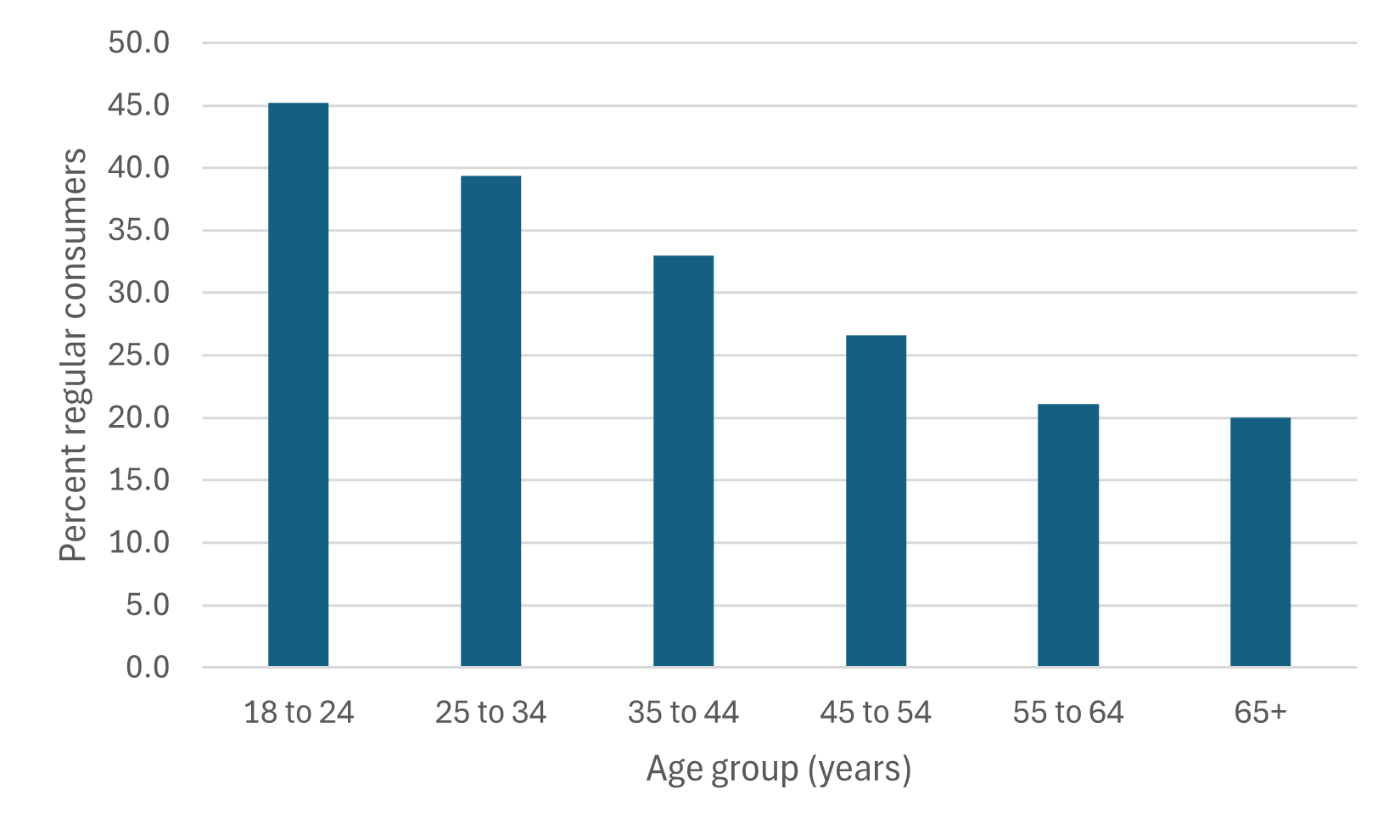
(a) Age

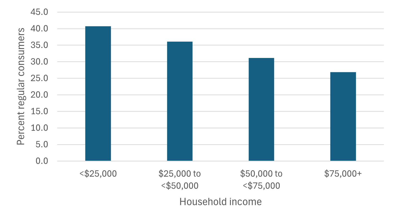
(b) Household income

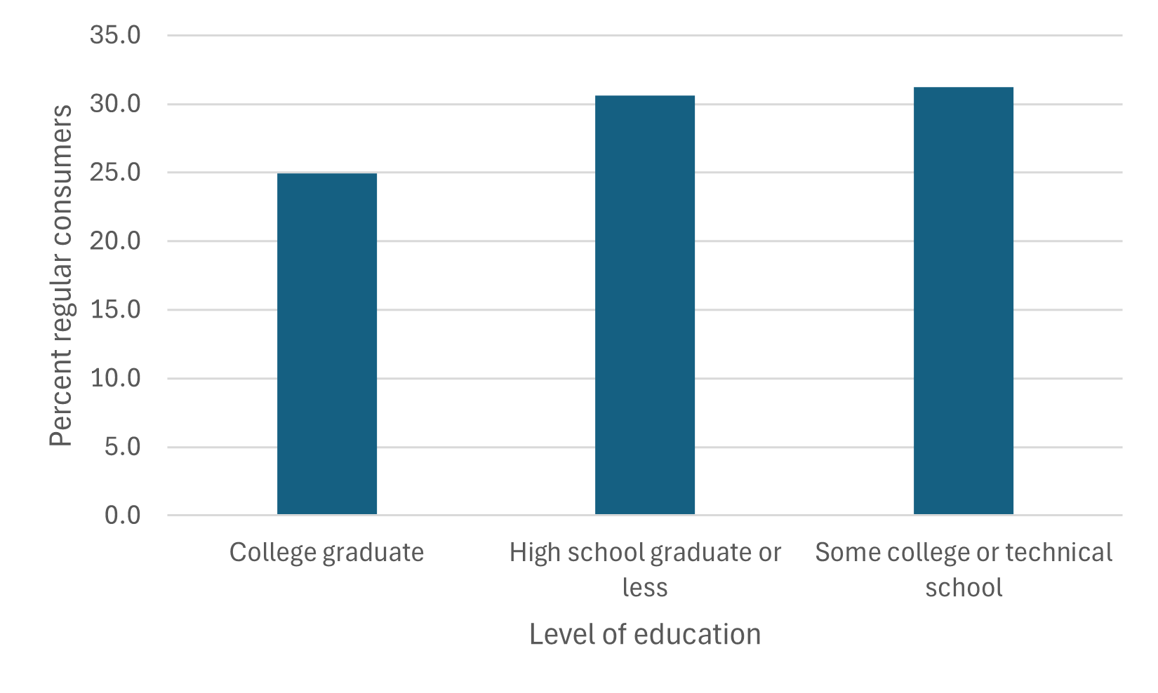
(c) Education

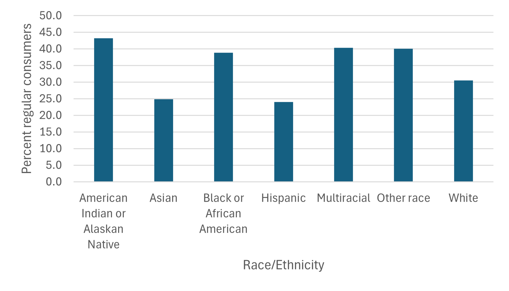
(d) Race/Ethnicity

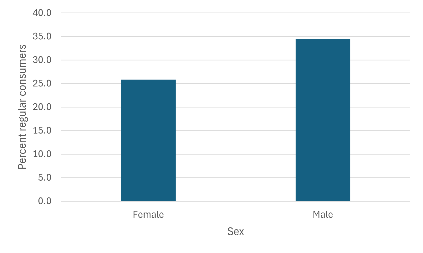
(e) Sex

  Notes: This figure presents the distribution of regular cannabis consumers in Washington state, broken down by various demographic characteristics: (a) age, (b) household income, (c) education level, (d) race/ethnicity, and (e) gender. Each bar represents the proportion of regular cannabis consumers within the respective subgroup. The data is from the 2021 Behavioral Risk Factor Surveillance System by the Washington State Department of Health, Center for Health Statistics.

The cannabis supply chain

Figure 5 shows the stages of the cannabis supply chain. Most cannabis in Washington is grown in indoor facilities ranging in size from 2,000 to 30,000 square feet of plant canopy. When plants reach a mature stage, their buds are harvested, dried, and cured. The majority of cannabis is consumed in this unprocessed form (called ”Usable marijuana”) while the rest is processed into derivative subproducts like edibles and concentrates.

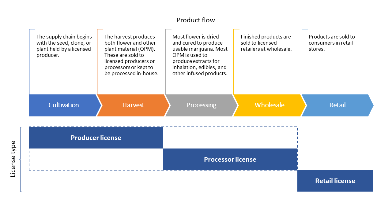
Figure 5: The cannabis supply chain

  Notes: This figure depicts the flow of cannabis products, from left to right, as they move through the supply chain. Only licensed producers are permitted to cultivate and harvest cannabis plants; producers can only sell to licensed processors, who in turn are permitted to process products; only processors can sell finished products at wholesale to retailers; licensed retailers can sell finished products to end consumers. An establishment can jointly hold producer and processor licenses, so the overwhelming majority of upstream establishments hold both licenses (i.e. producer-processors). Retailers may not hold a producer or a processor license and vice versa. As a result, production and retail activities are legally separated.

Store characteristics

Figure 6(c) shows the distribution of store-level monthly averages for various store characteristics. Panel (a) shows the average number of distinct products sold per month across stores. A 1.0 gram package and a 2.0 gram package of Sunset Sherbert usable marijuana (i.e. unprocessed dried flower) produced by Northwest Harvesting Co are examples of distinct products in our data. The average store in our sample sells 473 distinct products per month (median: 419). However, Panel (a) reveals substantial variation across stores in our sample, with values ranging from as low as 13 to a maximum of 1,833 products per month. Panel (b) reports the average units sold per month across stores (in thousands). The average store in our sample sells 14,836 units per month (median: 10,905). As is the case with product variety, there is large variation in units sold across stores. Stores at the 1st percentile sell 287 units per month, while those at the 99th percentile sell 72,826 units per month. Panel (c) shows the distribution of tax-inclusive monthly revenue across stores. The average store generates $285,320 revenue per month (median: $205,377). Again, revenue varies across stores: stores at the 1st percentile generate $3,765 while those at the 99th percentile generate $1,447,000 per month.

Figure 6: Distribution of monthly averages across stores

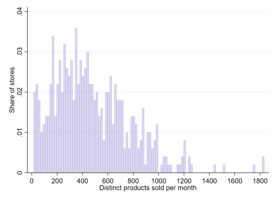
(a) Product variety

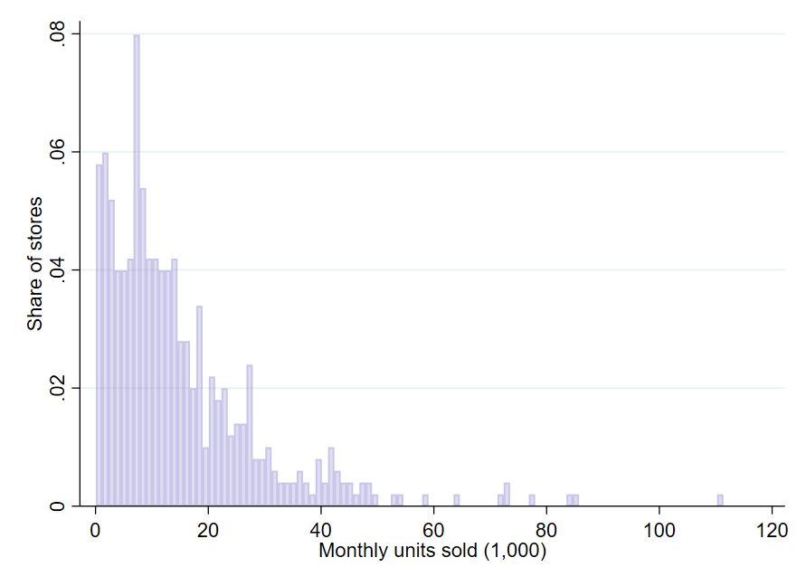
(b) Units sold

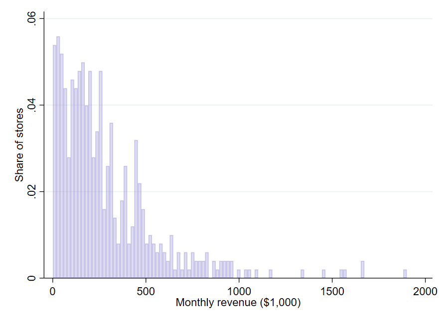
(c) Revenue (tax-inclusive)

  Notes: The figures show the distribution of store-level average statistics across all stores in our sample. Panel (a) presents the distribution of the average monthly number of unique products sold. Panel (b) displays the distribution of the monthly average units sold. Panel (c) illustrates the distribution of average monthly sales revenue across stores.

Variable cost structure for cannabis retailers

To ascertain the variable cost structure for cannabis retailers, we use aggregate payroll data on cannabis retailers from the Washington State Employment Security Department (ESD) and High Peak Strategy. The ESD collects data on employment and wages in industries covered by unemployment insurance (95 percent of U.S. jobs). The data spans the years 2018-2020. Table 7 illustrates that cannabis retailers have a similar variable cost structure as other retail industries studied in the literature. Renkin et al., (2022), for example, find that for U.S. grocery stores, COGS accounts for 83% of variable costs. Note that in most retail settings, cost of goods sold (COGS) and labor cost together account for 99% of variable cost while other expenditures like packaging and transport typically make up less than 1% of variable cost (Renkin et al.,, 2022).

Table 7: COGS and the labor share of costs for cannabis retailers

	Average expenditure		Variable cost share
Year	Labor	COGS	Labor	COGS
2018	$324,582	$702,358	0.32	0.68
2019	$370,897	$1,187,462	0.24	0.76
2020	$407,273	$1,584,301	0.20	0.80

Notes: This table compares average annual labor expenditure and COGS expenditure for cannabis retail stores in Washington state for the years 2018-2020. Aggregate payroll data on cannabis retailers is from the Washington State Employment Security Department and High Peak Strategy (2018-2020). Labor expenditure equals total wages divided by the number of active stores. Stores with missing UI data are excluded from total wages and establishment counts. COGS is the average annual wholesale expenditure for cannabis retailers in the estimation sample. Wholesale purchases from processor-only licenses are included.

The geography of wholesale costs

Table 8 shows the percentage of retailers’ wholesale costs in relation to a producer’s geographic location. Column 1 shows that only 5.22% of retailers’ wholesale expenditures go to producers located in the same city as the retailer. Column 2 shows that less than 15% goes to producers in the same county as the retailer. For Column 3, we sort counties into their respective 3-digit zip codes (retailers are located in 14 3-digit zip codes compared to 37 counties). Column 3 shows that less than 16% of wholesale cost goes to producers located in the same 3-digit zip code. Next, we sort counties into three regions (west, central, east), defined by well-established topographic and economic boundaries. Column 4 shows that 62% of wholesale sales go to retailers in a different region than the producer. Column 5 looks at the subset of establishments located in the west and east regions of the state, thus dropping producers in the central region. The east and west regions are non-contiguous and are located on opposite sides of the state. For establishments located in these two regions, 23.9% of wholesale sales go to retailers located in the other region, that is to say, retailers on the opposite side of the state. Because the majority of retail establishments are located in the west and east regions, this share amounts to 21.4% of all of wholesale expenditures in the industry. Taken together, the results from Table 8 illustrate that there is no home bias in wholesale cannabis purchases.

Table 8: Share of retailers’ wholesale costs by geographic proximity

	(1)	(2)	(3)	(4)	(5)	(6)
	Same city	Same county	Same 3-digit zip code	Same region	Non-contiguous region	Same state
Percent of wholesale expenditure	5.22%	14.67%	15.59%	62.08%	23.90%	100%

Notes: This table shows the share of retailers’ wholesale expenditure according to wholesalers’ geographic proximity. The shares are based on 5.92 million unique wholesaler-retailer-product-month observations from August 2018 through July 2021. Retailers are located in 14 3-digit zip codes and 35 counties. Region groups counties into three categories: west, central, or east. Data from Top Shelf Data.

Seasonality of crimes

Table 7 illustrates the seasonality in treatment timing within our sample. Each bar represents the number of crimes that occurred in the respective calendar month, with 1 indicating January and 12 indicating December. The figure shows that crime occurs throughout all months but that rates tend to be higher towards the end of the year.

  Notes: This figure illustrates the seasonality in treatment timing within our sample. Each bar represents the number of crimes that occurred in the respective calendar month, with 1 indicating January and 12 indicating December.

Appendix B Establishment-level indexes

This section provides more detial on the store-level indexes used in our analysis.

B.1 Price indexes

Our empirical analysis uses traceability data provided by the data analytic firm Top Shelf Data (TSD), which ingests the raw tracking data from the Washington state Liquor and Cannabis Board (LCB) and matches it with additional product information. Note that the raw tracking data from the LCB includes each product’s SKU, but TSD does not report this. Instead, each product is identified by a unique combination of five elements: retailer-producer-category-product name-unit weight. For products with no unit weight (such as liquid edibles), the first four elements identify the product. TSD then calculates the average price of product $i$ at retail store $j$ in month $t$ as

$$P_{i,j,t}=\frac{TR_{i,j,t}}{TQ_{i,j,t}}.$$ (8)

where $TR_{i,j,t}$ is the revenue from product $i$ at retailer $j$ in month $t$, and $TQ_{i,j,t}$ is total quantity.

To construct store-level price indexes, we employ a two-step process similar to that used by Renkin et al., (2022). In the first step, we use $P_{i,j,t}$ to construct a geometric mean of month-over-month changes for product subcategory $c$ at store $j$:

$$I_{c,j,t}=\prod_{i}\left(\frac{P_{i,j,t}}{P_{i,j,t-1}}\right)^{\omega_{i,c,j,y(t)}}$$ (9)

where each subcategory is a unique category-unit weight combination. For example, usable marijuana is a category, whereas 1.0 gram usable marijuana and 2.0 gram usable marijuana are separate subcategories. Following Renkin et al., (2022), the weight $\omega_{i,c,j,y(t)}$ is the share of product $i$ in total revenue of subcategory $c$ in establishment $j$ during the calendar year of month $t$.

In the second step, we aggregate across subcategories to get the price index for store $j$ in month $t$:

$$I_{j,t}=\prod_{c}I_{c,j,t}^{\omega_{c,j,y(t)}}.$$ (10)

Similar to the first step, the weight $\omega_{c,j,y(t)}$ is the share of subcategory $c$ in total revenue in store $j$ during the calendar year of month $t$. The store-level inflation rate is then simply the natural logarithm of the index

$$\pi_{j,t}=\ln I_{j,t}$$ (11)

B.2 Quantity indexes

The quantity indexes are constructed the same way as the price indexes. The only difference is in the first step

$$I_{c,j,t}=\prod_{i}\left(\frac{Q_{i,j,t}}{Q_{i,j,t-1}}\right)^{\omega_{i,c,j,y(t)}}$$ (12)

where $Q_{i,j,t}$ is the quantity sold of product $i$ at store $j$ in month $t$. The index weights are otherwise identical to those from the price index.

B.3 Wholesale cost indexes

The wholesale cost indexes are constructed similar to the price indexes. TSD calculates the average monthly wholesale price at the SKU-level as

$$W_{i,j,t}=\frac{TE_{i,j,t}}{TQ_{i,j,t}}.$$ (13)

where $TE_{i,j,t}$ is the total expenditure on product $i$ at retailer $j$ in month $t$, and $TQ_{i,j,t}$ is total quantity purchased at wholesale. In the first step of the establishment-level cost index, we construct a geometric mean of the month-over-month changes in wholesale price for product subcategory $c$ at store $j$:

$$I_{c,j,t}=\prod_{i}\left(\frac{W_{i,j,t}}{W_{i,j,t-1}}\right)^{\omega_{i,c,j,y(t)}}$$ (14)

where the subcategories are the same as before. In contrast to the price indexes, $\omega_{i,c,j,y(t)}$ is an expenditure weight equal to the share of product $i$ in the wholesale expenditure of subcategory $c$ at store $j$ in the calendar year of month $t$. Note that by calculating this weight based on annual (rather than monthly) expenditure shares, we may not capture short-term wholesale substitution patterns on the part of retailers. To check this, we also construct the index using monthly expenditure shares. This increases the variance of the indexes but does not change our main estimation results. Therefore, we use the annual expenditure weights for our preferred specification.

In the second step, we aggregate across subcategories to get the wholesale cost index for store $j$ in month $t$:

$$I_{j,t}=\prod_{c}I_{c,j,t}^{\omega_{c,j,y(t)}}.$$ (15)

Similar to the first step, the weight $\omega_{c,j,y(t)}$ is the share of subcategory $c$ in total wholesale expenditure in store $j$ during the calendar year of month $t$. The store-level wholesale cost index is then simply the natural logarithm of the index, $\ln I_{j,t}$.

B.4 Margins indexes

The margins indexes are constructed in a similar manner as the other indexes. Margins at the store-product-month level are defined as the ratio of the retail and wholesale prices

$$M_{i,j,t}=\frac{P_{i,j,t}}{W_{i,j,t}}$$ (16)

As with the other indexes, we construct a geometric mean of the month-over-month changes in margins for product subcategory $c$ at store $j$:

$$I_{c,j,t}=\prod_{i}\left(\frac{M_{i,j,t}}{M_{i,j,t-1}}\right)^{\omega_{i,c,j,y(t)}}$$ (17)

where the subcategories are the same as before. the weights are the same as those from the price index, i.e. based on annual revenue shares.

In the second step, we aggregate across subcategories to get the margins index for store $j$ in month $t$:

$$I_{j,t}=\prod_{c}I_{c,j,t}^{\omega_{c,j,y(t)}}.$$ (18)

The weight $\omega_{c,j,y(t)}$ is the share of subcategory $c$ in total revenue in store $j$ during the calendar year of month $t$. The store-level margins index is the natural logarithm of the index, $\ln I_{j,t}$.

Figure 8 shows the distributions for our indexes. For visual clarity, we omit extreme outliers that are otherwise included in our regressions. All four panels show that the distributions are centered at or near zero. Note that the quantity index has a higher variance than the other indexes. This is a common characteristic of indexes based on store-level scanner data and is similar to the findings of (Renkin et al.,, 2022; Leung,, 2021). The wholesale cost index has a comparatively smaller variance, reflecting the relative stability of wholesale cannabis prices.

Figure 8: Distributions for store-level indexes

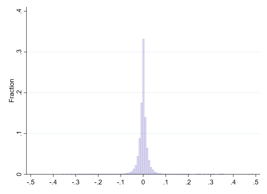
(a) Price

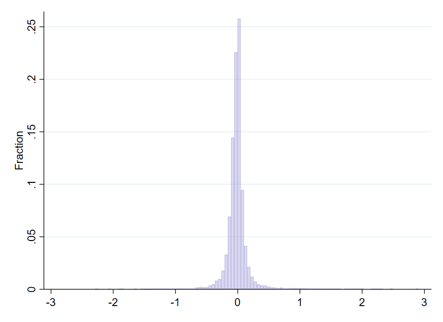
(b) Quantity sold

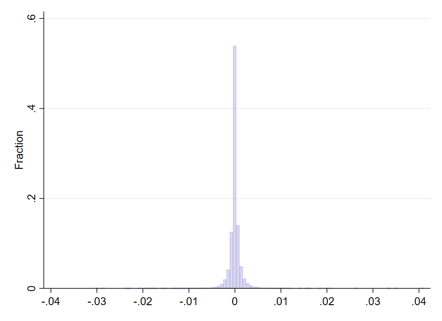
(c) Wholesale cost

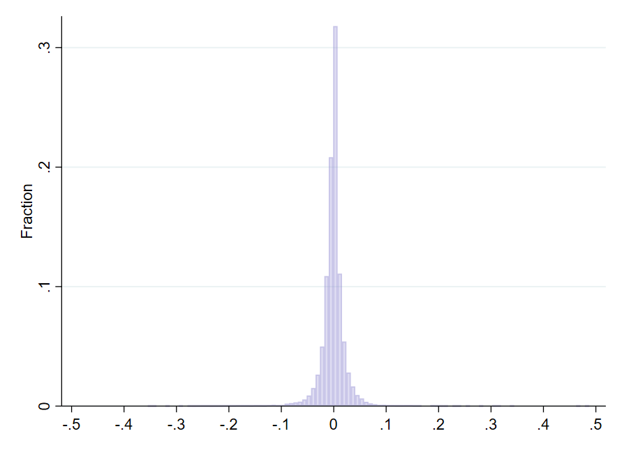
(d) Retail margins

  Notes: The figures show the distribution of the main dependent variables over the sample period. Panel (a) depicts the monthly store-level price index. Panel (b) illustrates the monthly store-level quantity index. Panel (c) displays the monthly store-level wholesale cost index. Panel (d) presents the monthly store-level retail margins index. For visual clarity, extreme outliers are omitted from the figures, although they are included in our regressions.

Appendix C Additional Heterogeneity Analysis

C.1 Descriptive statistics

Table 9: Market concentration descriptive statistics

	(1)	(2)	(3)
	Mean	Median	Std
Victimized HHI	0.15	0.11	0.19
All HHI	0.27	0.15	0.28

Notes: The table shows descriptive statistics for our market concentration measure, calculated on the store-level. The first row only considers victimized stores. the second row considers all stores withing the Washington State cannabis industry.

Table 10: Chain store characteristics

	(1)	(2)
	Independent	Chains
Unit price (in dollars)	26.74	26.78
	(4.29)	(4.58)
Units sold per month	13,421	16,161
	(13,068)	(15,399)
Monthly revenue (in dollars)	257,473	312,154
	(252,444)	(301,285)
Unique products per month	460	553
	(379)	(391)
$N$	330	181

Notes: The table reports descriptive statistics for chains and independent stores in our sample, as defined in the main paper. Standard deviations are in parentheses. The variables reported are: unit price, average store quantity sold per month, average store revenue per month, and average number of distinct products sold per month.

First versus subsequent crime incidents

In our main analysis, we concentrate on the first store-level crime incident during our observation period, meaning stores with multiple crime incidents are dropped from the sample prior to their second incident. In this subsection, we compare the effect on prices after the first incident at a store with that from subsequent (i.e. non-first) incidents at stores that had already experienced a crime. Of the 57 victimized stores in our sample period, 12 stores have multiple crime incidents: nine were victimized twice and three were victimized four times. Panel (a) in Figure 9(b) shows that the effect at victimized stores is not statistically significantly different from zero following a subsequent crime. The smaller number of subsequent crimes reduces the precision of our estimates, particularly towards the end of the event window. We conduct a similar analysis for rival stores. Dropping each rival store’s first treatment from the sample reduces the number of rival treatments from 264 to 94. Panel (b) shows that the price effect at rival stores falls from 1.7% percent to 0.7%. The effect remains statistically significant at the 10% level, which is likely due to the fact that numerous rivals stores are subsequently treated 1-2 months after their first treatment, so that removing the first treatment does not entirely eliminate the novelty of nearby crime incidents.

Overall, subsequent crime incidents have a smaller effect on prices at both victimized and rival stores compared to first crime incidents. This is consistent with the idea that subsequent crime incidents are not novel and do not induce stores to update their expectations over future crime incidents to the same degree as the first crime incident. In contrast, the first store-level crime incident comes as a surprise, leading stores to update their expectations and inducing a larger cost shock.

Figure 9: Price effects of first versus subsequent crime incidents

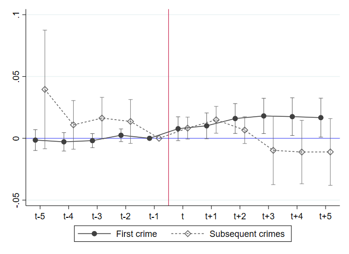
(a) Victimized stores

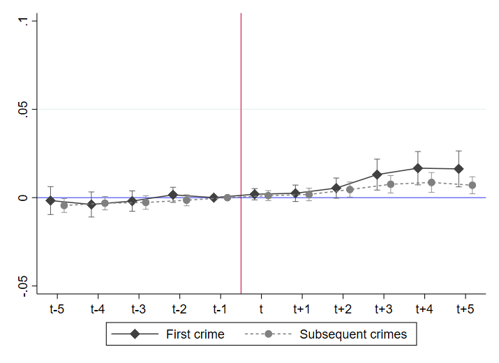
(b) Rival stores

  Notes: This figure shows the cumulative treatment effects ($E_{L}$) $L$ months after a crime on store price levels, along with corresponding 90% confidence intervals based on standard errors clustered at the store level. Coefficients are interpretable as percentage increases in outcome levels relative to the month before a crime incident. The black line shows the cumulative effects of the first crime per victimized store on price levels, i.e., our main specification. The dotted line illustrates the treatment effects of subsequent crimes at stores that experienced multiple crime incidents.

C.2 Additional results

Independent versus chain stores

In Table 11 we report alternative specifications for our heterogeneity analyses. In Section 5.2, we distinguished between small and large chains, with the former defined as stores belonging to firms with 1-2 stores and the latter corresponding to three or more stores. Now, we instead distinguish between independent stores (i.e. stores belonging to a single-store firm) and chain stores (stores at firms with two or more stores). Columns 1 and 5 show that effects at independent stores are smaller than the effects at small chains found in Section 5.2. Moreover, Columns 2 and 6 show a larger the effect at chains than in those found in Section 5.2. This redistribution of treatment effects reflects that stores in small chains have a large treatment effect that is similar in magnitude to independent stores. This points to small chain stores facing similar competitive pressures as independent stores, and validates our distinction between small and large chains in our main heterogeneity analysis in Section 5.2.

Market concentration

In Section 5.2, we found large effects at stores in markets with low concentration, and no effect at markets with high concentration. One possible reason for this finding is that low concentration markets are generally located in urban areas, where labor costs (and hence the security cost shock) may be higher compared to rural areas. To test this, we use an alternative definition of low and high concentration markets that accounts for urban-rural heterogeneity. We proceed as follows. First, we categorize as urban stores that are located in the four largest and most densely populated cities (Seattle, Tacoma, Bellevue, and Spokane), and consider all other stores as rural. Next, we calculate the median HHI for stores in the urban subsample and the median HHI for stores in the rural subsample. We split the urban subsample into high concentration and low concentration parts, and do the same for the rural subsample. This leaves us with four subsamples: urban low concentration, urban high concentration, rural low concentration, and rural high concentration. Finally, we pool the high concentration subsamples into a single subsample, and the low concentration subsamples into another subsample. Our low concentration subsample thus contains stores in markets considered low concentration in an urban setting, but also stores in markets considered low concentration in a rural setting. Finally, we estimate our main regression equation separately for the high concentration and the low concentration subsamples. Columns 3-4 show that at victimized stores, the difference in effect sizes between low and high concentration markets is 0.016 and not statistically significantly different from zero. The difference in effect sizes in Section 5.2 is 0.030 and statistically significant. Thus, accounting for the urban-rural divide appears to explain at least some of the comparatively large effect size for low concentration markets found in Section 5.2. Column 7 of Table 11 shows that compared to the results from Section 5.2, the low concentration effect decreases for rival stores as well when accounting for the rural-urban divide. In Section 5.2 we found an effect of 0.022, whereas now the effect is 0.019. However, the effect in high concentration markets also falls (Column 8), and the difference between low and high concentration markets slightly increases when accounting for the rural-urban heterogeneity.

To summarize, for victimized stores, urban-rural heterogeneity appears to explain some of the heterogeneous effects for low and high concentration markets. However, for rival stores, results are less clear. On the one hand, the effect in low concentration markets decreases when accounting for rural-urban differences, while on the other hand, the effect actually increases slightly in high concentration markets.

Table 11: Heterogeneity analysis robustness checks

	Victimized				Rivals
	(1)	(2)	(3)	(4)	(5)	(6)	(7)	(8)
	Indep. stores	Chain stores	Low concentration	High concentration	Indep. stores	Chain stores	Low concentration	High concentration
$E_{0}$	0.016	0.0015	0.0094	0.0053	0.0031	0.0019	0.0021	0.0078
	(0.012)	(0.0033)	(0.0075)	(0.0052)	(0.0037)	(0.0019)	(0.0023)	(0.0054)
$E_{2}$	0.029**	0.0079	0.020*	0.013**	0.0092**	0.0054	0.0087**	0.0037
	(0.014)	(0.0052)	(0.010)	(0.0059)	(0.0046)	(0.0038)	(0.0037)	(0.0084)
$E_{4}$	0.034**	0.0072	0.024*	0.0085	0.019***	0.015**	0.019***	0.0070
	(0.016)	(0.0078)	(0.013)	(0.0070)	(0.0068)	(0.0061)	(0.0065)	(0.011)
$\sum\text{Pre-event}$	0.0070	-0.0072	-0.0044	0.0022	-0.0091	0.0026	0.0005	-0.0004
	(0.0066)	(0.0062)	(0.0057)	(0.0060)	(0.0072)	(0.0052)	(0.0054)	(0.010)
$N$	14,856	15,428	8,163	7,786	10,845	14,675	8,756	8,299

Notes: Each column shows the cumulative treatment effects on store price levels for different subsamples zero, two, and four months after a crime, along with the sums of pre-treatment coefficients. Coefficients are interpretable as percentage increases in outcome levels relative to the month before a crime incident. The first four columns use victimized stores as the treatment group, and the last four columns consider rival stores. Columns 1 and 5 show effects for independent stores (owned by firms running one store only), while columns 2 and 6 show effects for stores owned by firms running at least two stores. For the other columns, the Herfindahl-Hirschman Index, conditional on a store being located in a rural or urban area, is calculated for the market around each store (including non-treated stores) within a 5-mile radius. The sample is then split according to the median market concentration in rural and urban areas, respectively. Columns 3 and 7 show effects for treated stores in rural and urban markets with below median concentration, and columns 4 and 8 for treated stores in markets with above median concentration. Standard errors of the sums are clustered at the store level and shown in parentheses. ^∗ $p<0.10$, ^∗∗ $p<0.05$, ^∗∗∗ $p<0.01$.

Appendix D Strategic complementarity in pricing

In this appendix section, we discuss the implications and potential issues arising from strategic complementarity in pricing in our setting. Furthermore, we present estimation results measuring the extent of strategic pricing in the Washington state cannabis industry.

D.1 Theoretical framework

We follow the framework of Muehlegger and Sweeney, (2022) and consider the pass-through of a tax (or input cost shock) $\tau$ onto the price of firm $j$. Firm $j$ sets the profit-maximizing price $p_{j}$ and faces tax-inclusive marginal costs $\alpha_{j}$. Each firm in the market can have a different exposure to the tax, with $\frac{\partial\alpha_{j}}{\partial\tau}$ capturing the marginal unit tax rate faced by firm $j$. In oligopolistic markets, the price a firm sets is a function of not just its own costs, but also those of its rivals. The pass-through of the tax onto firm $j$’s price can thus be decomposed as a direct (own-cost) and an indirect (competitors’ cost) effect:

$$\frac{\partial p_{j}}{\partial\tau}=\frac{\partial p_{j}}{\partial\alpha_{j}}\frac{\partial\alpha_{j}}{\partial\tau}+\sum_{i\neq j}\frac{\partial p_{j}}{\partial p_{i}}\frac{\partial p_{i}}{\partial\alpha_{i}}\frac{\partial\alpha_{i}}{\partial\tau}$$ (19)

where $\frac{\partial p_{j}}{\partial p_{i}}$ is firm $j$’s best response to a change in firm $i$’s price. Consequently, in the presence of imperfect competition, the strategic response of (untreated) competitors may disqualify them as a valid control group.

D.2 Quantifying strategic complementarity in prices

To identify the scope of strategic complementary in prices, we follow the industrial organization literature that measures the pass-through of cost shocks and taxes. In particular, we build on the approach of Hollenbeck and Uetake, (2021), who use similar data to evaluate the optimal cannabis sales tax. A major advantage of this approach is that, because we observe wholesale unit prices, we can directly measure how changes in unit cost are passed through to prices. In addition to stores’ own wholesale unit costs, we also observe the wholesale unit costs of their competitors. By relating stores’ prices to competitors’ cost changes, we can measure the effect of competitors’ cost-induced price changes, i.e. strategic complementarity in prices. Moreover, we can test whether this effect is a function of the geographic distance between stores. We use the results of this analysis to define unaffected local markets (a clean control inclusion criterion in Section 4).

To investigate the geographic scope of strategic complementarity of prices, we sort competitors into 5-mile bins and calculate average wholesale prices for each store-product-month-bin. We specify a model at the store-product-month level that relates a store-product’s retail price to (i) the wholesale unit price and (ii) the average wholesale unit price paid by stores in each distance bin. By including both own costs and competitors’ costs, we capture the total effect (i.e. own-cost and strategic price response) of an aggregate unit cost shock on stores’ prices. Since cannabis transaction data is publicly available, stores have full information on competitors’ unit costs and prices updated on an almost weekly basis. Therefore, we focus on contemporaneous changes in costs and prices. This is in line with the pass-through literature from other industries (see e.g. Hollenbeck and Uetake,, 2021; Muehlegger and Sweeney,, 2022; Conlon and Rao,, 2020; Miller et al.,, 2017). We estimate the following model in first-differences:

$$\Delta p_{i,j,t}=\rho\Delta w_{i,j,t}+\sum_{r=1}^{R}\beta_{r}\Delta w_{i,r(j),t}+\Delta\gamma_{t}+\Delta\varepsilon_{i,j,t},$$ (20)

where $p_{i,j,t}$ is the average price (in dollars) of product $i$ sold at store $j$ in month $t$, $w_{i,j,t}$ is the average wholesale price that retailer $j$ pays for product $i$ in month $t$, $w_{i,r(j),t}$ is the average wholesale price that competitors pay for product $i$ in month $t$, and $\gamma_{t}$ is the year-month FE. In our baseline specification, we set $R=12$ (setting $R\neq 12$ does not strongly affect estimates but changes the sample size and standard errors). We cluster standard errors at the store level to allow for autocorrelation in unobservables within stores.

The overall effect of the aggregate cost shock on store $j$’s prices comprises two parts: (i) the own cost pass-through rate, and (ii) the competitors’ cost pass-through rate (i.e. the strategic price response). The own cost pass-through rate, $\rho$, is the increase in unit price at store $j$ from the increase in store $j$’s own unit cost. The coefficient $\beta_{r}$ measures the pass-through of wholesale unit costs at competing stores in bin $r$ to unit prices at store $j$. This is equivalent to the strategic price response between store $j$ and competing stores in bin $r$. Thus, $\beta_{1}$ is the strategic price response for stores within 0-5 miles of store $j$, $\beta_{2}$ is the additional strategic price effect attributable to stores 5-10 miles away, and so on.

In addition to our main specification, we estimate several variants of our pass-through regression. First, we estimate equation 20 in levels rather than first-differences, with store-product FE. Second, we specify equation 20 using the first-difference of logs. This minimizes the influence of outliers and delivers pass-through elasticities instead of pass-through rates.

In Figure 10(c), we report estimated pass-through rates of competitors’ unit costs for each distance bin $r\in[1,12]$. Panels (a) and (c) show increasing marginal strategic complementary in prices up to the 30-mile mark. The fact that the effect increases with distance may reflect commuting patterns, with the average daily distance travelled in Washington state ranging from less than 20 miles in some counties to more than 70 in others (Axios,, 2024). Beyond 30 miles, the incremental effect of increasing the scope of the cost shock drops to zero for three consecutive bins. Interestingly, in panel (c) the 45-50 mile bin is positive and significant at the 10% level, though approximately half the size of the largest coefficients within 30-miles. Panel (b) shows some evidence of strategic complementarity in prices up to the 30-mile mark, again with effects that drop to zero for three consecutive bins thereafter.

Figure 10: The pass-through of competitors’ unit costs to own unit prices

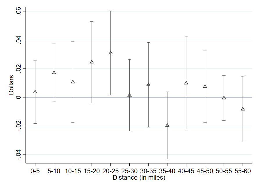
(a) Dollars, first-differenced

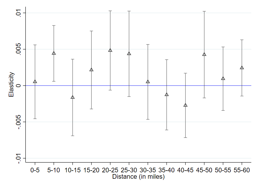
(b) First difference of logs

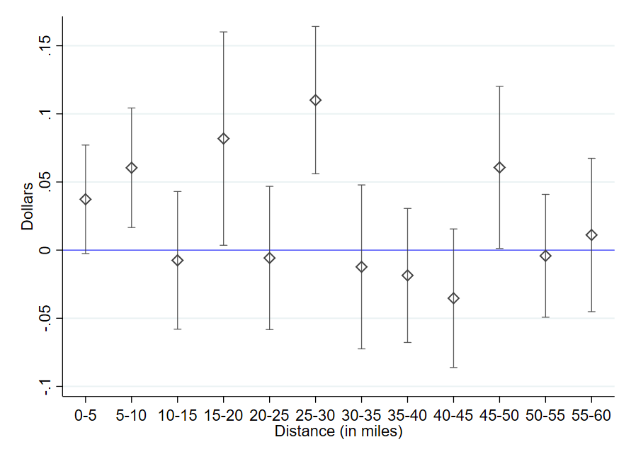
(c) Dollars

  Notes: the figures shows cumulative sums of coefficients $\sum_{r=1}^{R}\beta_{r}$ for $R\in[1,12]$, obtained from the pass-through regression (equation 20). Panel (a) is estimated in dollars; Panel (b) is first-differences of dollars. Panel (c) is specified in logs; Panel (d) is first-differences of logs. The figure shows 90% confidence intervals of the sums based on SE clustered at the store level. Data: Top Shelf Data, March 2018 through December 2021.

The $\beta_{r}$ estimates in Figure 10(c) measure the additional effect on store $j$’s prices of increasing the geographic scope of an aggregate cost shock by another 5 miles. This is informative about the geographic scope of strategic complementarity in cannabis prices. However, to quantify the effect on prices of an aggregate cost shock, we report cumulative effects $\sum_{r=1}^{R}\beta_{r}$ at increasing distance bins in Table 12. Since effects change little beyond the 30-mile mark (see Figure 10(c)), we only report cumulative effects up to 45 miles. The results in Table 12 indicate that an aggregate cost with sufficient geographic scope shock has non-negligible strategic price effects. A $1 increase in wholesale unit costs at all stores within a 30-mile radius corresponds to a $0.09 (Column 1), $0.10 (Column 2), and $0.45 (Column 3) increase in a store’s retail price solely due to strategic complementarities. These effects are much larger than those from a cost shock affecting only rival stores (i.e. 0-5 miles) found in Table 6. This aligns with a growing literature showing that the scope of cost shocks matters and that aggregate (i.e market-wide) cost shocks elicit a larger strategic price response than idiosyncratic or highly localized shocks (Muehlegger and Sweeney,, 2022).

Table 12: Cumulative pass-through of competitors’ unit costs

	(1)	(2)	(3)
	Dollars (FD)	Logs (FD)	Dollars (levels)
Own wholesale cost	1.654***	0.712***	1.294***
	(0.035)	(0.008)	(0.375)
Competitors’ wholesale cost
$<5$ miles	0.004	0.001	0.068*
	(0.011)	(0.003)	(0.037)
$<10$ miles	0.021	0.005	0.174***
	(0.014)	(0.003)	(0.058)
$<15$ miles	0.031*	0.003	0.193**
	(0.018)	(0.004)	(0.081)
$<20$ miles	0.056**	0.005	0.300***
	(0.023)	(0.005)	(0.100)
$<25$ miles	0.087***	0.010**	0.319***
	(0.025)	(0.005)	(0.111)
$<30$ miles	0.088***	0.015***	0.449***
	(0.027)	(0.005)	(0.139)
$<35$ miles	0.097***	0.015***	0.474***
	(0.030)	(0.005)	(0.158)
$<40$ miles	0.077**	0.014***	0.470***
	(0.031)	(0.005)	(0.165)
$<45$ miles	0.087***	0.011**	0.422***
	(0.028)	(0.005)	(0.159)
$N$	2,012,861	2,012,861	3,239,632

Notes: The table reports estimates of pass-through rates of wholesale unit cost to retail unit price at the store-product-month level, according to equation 20. We report estimates for own wholesale cost changes and for average changes in wholesale costs at competing stores according to the distance-bins described in the main text. Competing store effects are cumulative sums $\sum_{r=1}^{R}\beta_{r}$. Coefficients are interpretable as the dollar increase in prices resulting the strategic price response from a $1 dollar wholesale cost shock affecting all stores within a given distance. Standard errors are clustered at the store level and shown in parentheses. ^∗ $p<0.10$, ^∗∗ $p<0.05$, ^∗∗∗ $p<0.01$

Overall, the results from Figure 10(c) and Table 12 provide suggestive evidence of strategic complementarity in prices for stores within 30 miles of each other. Increasing the geographic scope of an aggregate cost shock appears to have little additional effect on store prices beyond the 30-mile mark. This suggests that stores located more than 30 miles from a victimized store will not have a strategic price response to the crime-induced cost shock at victimized and rival stores. We therefore view Figure 10(c) and Table 12 as providing supportive evidence for our definition of unaffected local markets from Section 4.

Appendix E Spatial treatment and alternative estimators

E.1 Stacked DiD with spatial treatment

One advantage of the stacked DiD estimator, compared to other estimators that address biases from staggered treatment adoption (e.g. Callaway and Sant’Anna,, 2021; Borusyak et al.,, 2024), is that rules defining clean controls readily extend to geographic criteria. This feature allows us to mitigate biases from spillovers to untreated stores and/or differences between stores, while at the same time ensuring a large number of clean control stores. In contrast, with alternative estimators (including canonical TWFE) restrictions on the control group composition must be imposed for the entire sample period, which considerably decreases the number of valid control observations.

To illustrate how our stacked DiD estimator addresses spillover effects, we provide a simple example in Figure 11. The figure depicts four stores: A and B are both victimized while stores C and D are not victimized. Concentric rings of diameter $\underline{d}$ and $\overline{d}$ denote the boundaries for control candidates for the victimized stores. Store C is a control candidate for both A and B while store D is a control candidate for B only. Since D is in another store’s inner ring (that of store A) it is not a clean control: if the event windows for stores A and B overlap, D is disqualified from the control group for both stores. However, store D qualifies as a clean control for store B if the event windows for stores A and B do not overlap. This reflects that store D’s contamination from store A’s treatment is zero outside of store A’s treatment window. Similarly, an earlier-treated store would qualify as a control store for a later-treated store if the earlier-treated store is in the later-treated’s outer ring and the event windows do not overlap. Store C qualifies as a clean control for both stores A and B because it is in the outer ring for both stores. This holds even if the event windows for store A and B overlap, since store C is unaffected by either store’s treatment.

Figure 11: Clean controls

  Notes: The figure depicts the locations of four stores (A, B, C, D) in relation to each other. Stores A and B are victimized while stores C and D are not. Concentric rings of diameter $\underline{d}$ and $\overline{d}$ denote the boundaries defining clean control stores in our setting.

Using the intuition from Figure 11, we can formally express the inclusion criteria for clean controls in our stacked DiD design. Let $J$ be the set of all stores in our sample, $t_{j}$ is the month that store $j$ is victimized, $w$ is the size of the event window (in months), $d_{k,j}$ is the geodesic distance between stores $j$ and $k$ (in miles). Store $i$ qualifies as a clean control if the following conditions jointly hold:

1. IC.1: $i\notin T_{j^{-}}$, where $T_{j^{-}}=\{k\in J,k\neq j:(t_{k}+w<t_{j})\lor(t_{k}-w>t_{j})\}$

2. IC.2: $i\in O_{j}$ where $O_{j}=\{k\in J:\underline{d}\leq d_{k,j}\leq\overline{d}\}$

3. IC.3: $i\notin D_{T_{j^{-}}}$, where $D_{T_{j^{-}}}=I_{j^{-}}\cap T_{j^{-}}$, and $I_{j^{-}}=\{k\in J:d_{k,j}<\underline{d}\}$

Condition IC.1 requires that store $i$’s treatment window does not overlap with that of store $j$. This is the standard stacked DiD inclusion criterion that prevents unclean comparisons between early- and late-treated stores. Condition IC.2 requires that store $i$ be located between $\underline{d}$ and $\overline{d}$ miles of store $j$. This is the geographic criterion that designates, e.g., stores C and D as candidate controls for store B in Figure 11. Condition IC.3 requires that store $i$ not be located within $\underline{d}$ miles of any treated store whose event window overlaps with that of store $j$. Condition IC.3 ensures two things. First, it imposes the geographic criterion that disqualifies store D as a clean control for store A in Figure 11. Second, it extends this criterion along the time dimension so that store D nevertheless qualifies as a control candidate for store B if store B’s event window does not overlap with that of store A.

If store $i$ satisfies all three conditions (IC.1-IC.3) then it qualifies as a clean control for store $j$ and is included in the sub-experiment corresponding to the crime incident at store $j$. Before moving on, it is worth highlighting two points. First, store $i$ may satisfy IC.1-IC.3 for some crime incidents but not for others. As long as store $i$ satisfies all three criteria for a given crime incident, then it will be included in that sub-experiment. Second, store $i$ may qualify as a clean control for multiple sub-experiments that overlap in calendar-time. This is a common feature of the stacked DiD estimator and it implies that certain store-month observations may be recycled and appear in multiple sub-experiments (Wing et al.,, 2024). For example, in Figure 11, if stores A and B are both victimized in the same period, then store C serves as a clean control for both sub-experiments (assuming the other conditions are satisfied). Store C is then included in each of the sub-experiment-specific datasets, meaning the stacked dataset will contain duplicate observations for store C for the calendar months corresponding to that particular event window.

Alternative estimators

To assess whether our findings are sensitive to the choice of estimator, we use three alternative approaches: i) the canonical two-way fixed effect Difference-in-Differences estimator (TWFE) prone to biases under staggered treatment adoption; ii) the imputation estimator developed by Borusyak et al., (2024) (BSJ); and iii) the estimator proposed by Callaway and Sant’Anna, (2021) (CS). We estimate all models separately for both of our treatment groups (victimized and rival stores). Similar to our main specification, we first estimate a distributed lag model for the same event window (equation 2) and then calculate the cumulative treatment effects using the period before treatment as our reference period.

The underlying dataset for the alternative estimators includes all stores, which means the control group may comprise stores within 30 miles of victimized stores, potentially introducing biases due to spillover effects. Accordingly, positive price effects at these stores would imply that we underestimate the treatment effects in these models. If we would restrict the sample to all stores that are located more than 30 miles from any treated stores, the number of clean control stores falls from 329 to 78 stores, demonstrating the advantages of the stacked DiD framework in our setting.

For the BSJ estimator, we use the accompanying Stata package ”did_imputation” from Borusyak et al., (2024). Standard errors allow for clustering at the store level. We calculate standard errors (detailed in Borusyak et al., (2024)) using the treatment effect averages across treatment cohorts (time since treatment) excluding the own unit. For the CS estimator, we employ the Stata package ”csdid” with clustered, asymptotic standard errors and stabilized inverse probability weighting. For both estimators, we consider all never-treated and not-yet-treated stores as potential control observations.

One notable difference among the estimators is the benchmark against which the average distributed lag coefficients are calculated. The canonical TWFE, similar to our main specification, calculates the distributed lag coefficients relative to the last period before the event window. The CS estimator uses the last pre-treatment period as a reference, while BJS bases its comparison on the average of all pre-treatment periods (Roth et al.,, 2023). If all benchmarks were zero, these differences would be irrelevant. However, since the last pre-treatment period coefficient is slightly negative, the cumulative coefficients from the CS estimator turn out to be higher than those from other estimators. For the CS estimators, we employ ”long” differences, yet the interpretation of pre-treatment coefficients still varies slightly between BSJ and other estimators. Importantly, all distributed lag coefficients are insignificant, and pre-tests included in the packages reveal no concerning pre-trends.

Table 13 shows the cumulative treatment effects at $k=0$, $k=2$, and $k=4$ for the alternative estimators. As anticipated, the treatment effects are generally smaller than those in our main specification. The effect size is approximately 1.5% for victimized stores and around 1% for rival stores, except in the CS specification for victimized stores that shows higher effects. For victimized stores, all effects become statistically significant two periods after treatment. For rival stores, effects materialize with some delay, becoming significant after four periods in the TWFE and BSJ specifications, but not in the CS estimation. Overall, this evidence supports our conclusion that the effects of crime on prices are robust and not dependent on the choice of estimator.

Table 13: Alternative estimators

	Victimized			Rivals
	(1)	(2)	(3)	(4)	(5)	(6)
	TWFE	BJS	CS	TWFE	BJS	CS
$E_{0}$	-0.001	-0.001	0.009	0.001	0.002	0.002
	(0.004)	(0.005)	(0.006)	(0.002)	(0.002)	(0.003)
$E_{2}$	0.010**	0.016***	0.025**	0.003	0.004	0.007
	(0.004)	(0.006)	(0.011)	(0.003)	(0.003)	(0.007)
$E_{4}$	0.014*	0.016**	0.035**	0.010**	0.010*	0.015
	(0.008)	(0.007)	(0.017)	(0.004)	(0.005)	(0.012)
$\sum\text{Pre-event}$	-0.001	-0.001	0.012	-0.001	-0.002	0.001
	(0.005)	(0.006)	(0.012)	(0.004)	(0.005)	(0.010)
N	17,606	17,110	17,517	17,606	13,489	16,698

Notes: Each column shows the cumulative treatment effects on store price levels zero, two, and four months after a crime using different alternative estimators, along with the sums of pre-treatment coefficients. Coefficients are interpretable as percent increases in store price levels relative to the month before a crime incident. Columns 1-3 use victimized stores as the treatment group, while Columns 4-6 consider rival stores. Columns 1 and 4 estimate our regression equation using the canonical two-way fixed effects estimator. Columns 2 and 5 employ the imputation estimator proposed by Borusyak et al., (2024). Columns 3 and 6 show cumulative treatment effects using the estimator developed by Callaway and Sant’Anna, (2021). Standard errors, which allow for clustering at the store level, are reported in parentheses. ^∗ $p<0.10$, ^∗∗ $p<0.05$, ^∗∗∗ $p<0.01$.

Appendix F Additional robustness checks

Placebo tests

We conduct several placebo tests to check for a potential violation of the parallel trends assumption. We shift treatment assignment forward by 12 months and estimate our main empirical equation (equation 2) with leads and lags based on this placebo treatment assignment. In a second test, we shift treatment timing back by 12 months. If either of these placebo treatment timings were to produce large and and statistically significant treatment effects, then this would cast doubt on our parallel trends assumption.

We report our placebo test estimates in Table 14. Column 1 shows that when the treatment timing for victimized stores is moved forward by 12 months, treatment effects are close to zero and statistically insignificant. Column 2 shows the effect at victimized stores when treatment timing is shifting back in time by 12 months. Columns 3 and 4 report the same tests for rival stores (with rivals defined as in the main text). In Column 4, the effect at rival stores in $t=0$ is significant at the 10% level. However, the effect size is small and is not stable over time, which eases our concerns. Note that the sample sizes in Columns 2 and 4 are reduced. This is because our scanner data only runs through December 2021; since more crimes occurred in the second half of the sample period, shifting treatment timing back in time results in a substantially reduced treated group (e.g. a store originally treated in August 2021 is assigned treatment in August 2022, which falls outside of the sample period). Overall, the results speak against a violation of the parallel trends assumption.

Table 14: Placebo tests

	Placebo
	(1)	(2)	(3)	(4)
	Vict. -12 months	Vict. +12 months	Rivals -12 months	Rivals +12 months
$E_{0}$	-0.000	-0.011	-0.002	-0.004*
	(0.004)	(0.009)	(0.004)	(0.003)
$E_{2}$	-0.001	-0.019	-0.004	-0.004
	(0.008)	(0.013)	(0.006)	(0.005)
$E_{4}$	0.004	-0.020	-0.002	-0.006
	(0.010)	(0.015)	(0.006)	(0.007)
$\sum\text{Pre-event}$	-0.007	-0.001	-0.003	-0.005
	(0.020)	(0.009)	(0.006)	(0.005)
$N$	11,015	7,827	10,897	8,393

Notes: Each column shows the cumulative placebo effects on store price levels for different subsamples zero, two, and four months after a placebo crime date, along with the sums of the corresponding pre-”treatment” coefficients. The placebo crime date is defined as 12 months before (Columns 1 and 3) or 12 months after (Columns 2 and 4) the actual crime date. Coefficients are interpretable as percentage increases in outcome levels relative to the month before a placebo crime incident. The first two columns use victimized stores as the treatment group, while the last two columns consider rival stores. Standard errors of the sums are clustered at the store level and shown in parentheses. ^∗ $p<0.10$, ^∗∗ $p<0.05$, ^∗∗∗ $p<0.01$.

Longer event window

Figure 12 illustrates that our main results carry over when we extend the event window from 11 months to 19 months. Prices at victimized stores rise for three months following a crime incident and maintain a higher level for nine months. Rival stores experience similar price increases, albeit with a two-month delay. The treatment effects remain largely unchanged beyond the original 11-month event window, reinforcing our empirical strategy’s assumption of constant treatment effects outside this period.

The effects on quantity sold (Panel (b)) are more volatile than those for price, reflecting the much larger variance for the quantity indexes compared to the other indexes. Pre-treatment, the effects at both victimized and rival stores are insignificant and show no significant differences. Interestingly, several months post-crime, we notice a decrease in quantities sold at both victimized and rival stores. This reduction is likely due to consumers shifting away from these stores in response to the higher prices. Initially, demand at these stores appears inelastic, but as consumers adjust to the increased prices, demand decreases as expected.

Panel (c) shows little effect on wholesale prices, as in the main section. As in the main section, the effects on margins (Panel (d)) closely resemble the price level effects, again reflecting the lack of wholesale price effects. Taken together, the results from Figure 12 illustrate that treatment effects materialize and stabilize well before $t+5$, which validates our choice of an 11-month event window for our main analysis in Section 5.

Figure 12: Effect of crime on store outcomes with extended event window

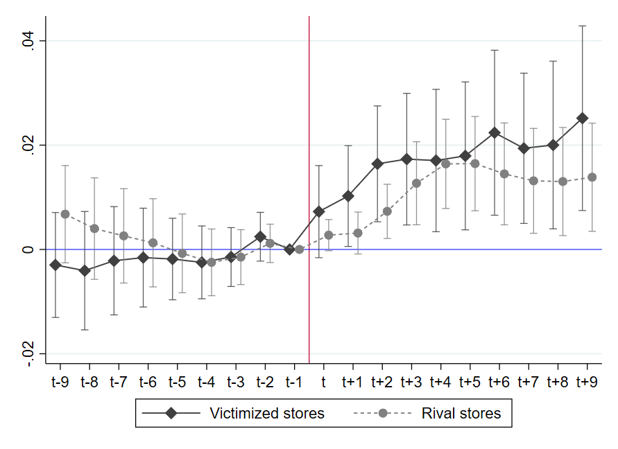
(a) Price level

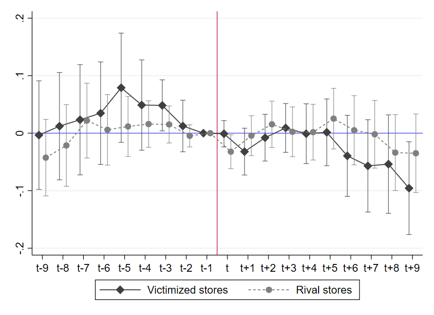
(b) Quantity sold

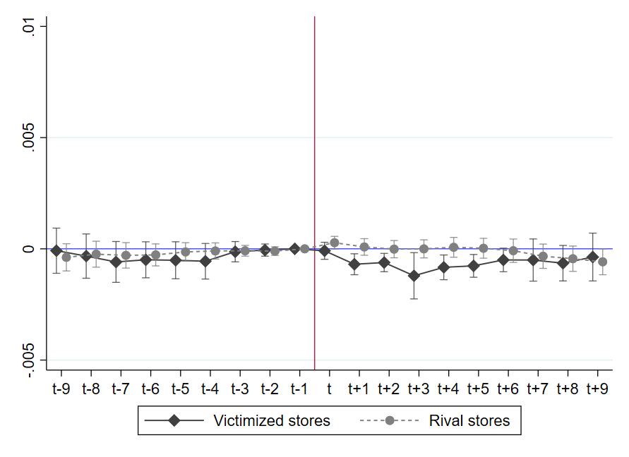
(c) Wholesale cost

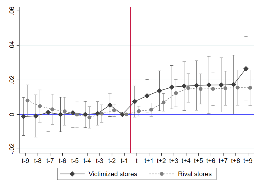
(d) Retail margins

  Notes: Each panel shows the cumulative treatment effects ($E_{L}$) $L$ months after a crime on different outcomes, along with corresponding 90% confidence intervals based on standard errors clustered at the store level. Compared to the main specification, we extend the event window from 11 to 19 months. Coefficients are interpretable as percentage increases in outcome levels relative to the month before a crime incident. The black line depicts the cumulative effects of crime on outcomes at victimized stores, while the grey line represents rival stores. The dependent variables are: store-level price index (Panel (a)), store-level quantity index (Panel (b)), store-level wholesale cost index (Panel (c)), and store-level margins index (Panel (d)).

Alternative inner vs. outer ring sizes

To investigate whether our estimated effects hinge on our definition of clean control stores, we estimate our model using alternative spatial definitions of clean control stores. Figures 13(a) and 13(b) show the cumulative treatment effects four months after a crime incident for victimized stores and for rival stores, respectively. The middle bar refers to our main specification. The first bar in both figures shows the effects when expanding the inner boundary to include all stores within 10 and 50 miles as potential control stores, and the third bar shows the effects of expanding the outer boundary to include all stores that are located more than 30 miles away from victimized stores.

Similarly, Figure 13(c) illustrates estimated effects as we expand the definition of the inner ring defining rival stores. The first bar reflects cumulative effects in our main specification; the second shows effects for stores within 10 miles, and the third for stores within 15 miles of victimized stores.

Figure 13: Price effects with alternative inner and outer rings

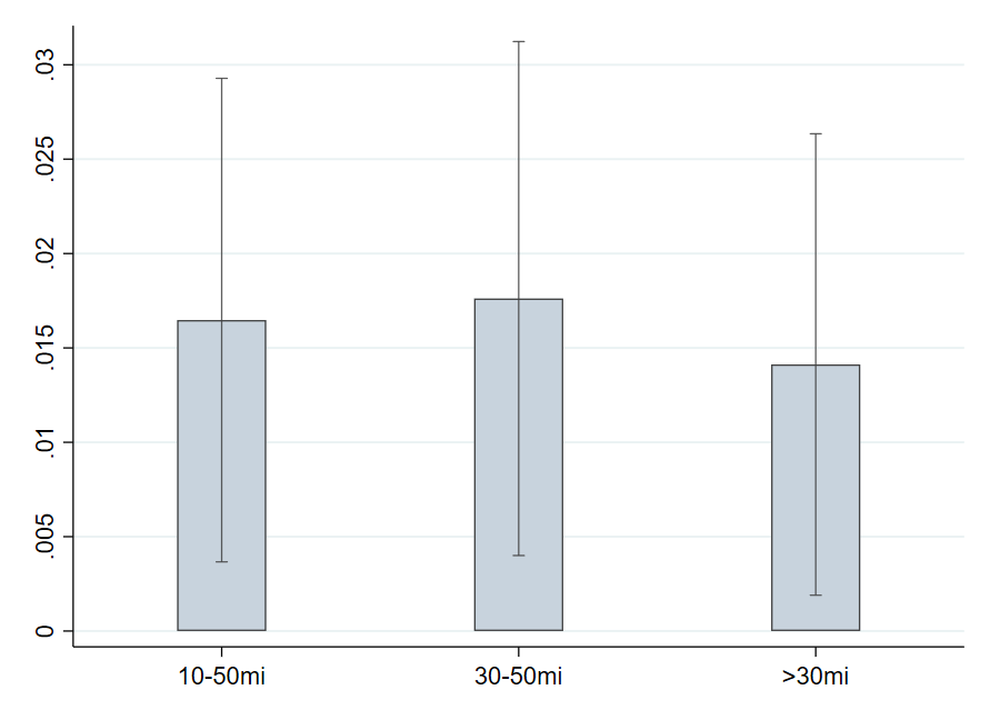
(a) Victimized stores, outer ring

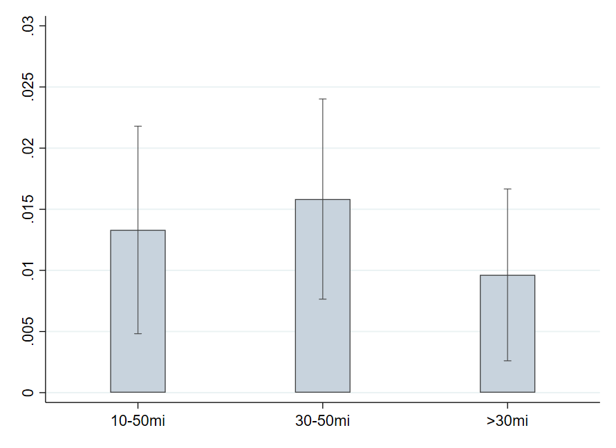
(b) Rival stores, outer ring

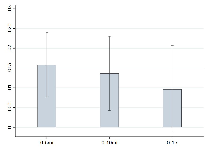
(c) Rival stores, inner ring

  Notes: Panels (a) and (b) show the cumulative treatment effects four months after a crime incident for victimized stores and for rival stores, respectively, along with corresponding 90% confidence intervals based on standard errors clustered at the store level. The first bar in both panels shows the effects when considering all stores within 10 and 50 miles as potential control stores. The middle bar refers to our main specification. The third bar shows the effects when considering all stores located more than 30 miles away from victimized stores as clean control stores. Panel (c) illustrates estimated effects as we expand the definition for rival stores. The first bar reflects cumulative effects in our main specification; the second bar shows effects when considering all stores within 10 miles as rival stores, and the third bar shows effects when considering all stores within 15 miles as rivals.

References

- Ambrose et al., (2021) Ambrose, C. A., Cowan, B. W., and Rosenman, R. E. (2021). Geographical access to recreational marijuana. Contemporary Economic Policy, 39:778–807.
- Axios, (2024) Axios (2024). Americans’ average daily travel distance, mapped. https://www.axios.com/2024/03/24/average-commute-distance-us-map. Retrieved April 24, 2024.
- Baker et al., (2022) Baker, A. C., Larcker, D. F., and Wang, C. C. (2022). How much should we trust staggered difference-in-differences estimates? Journal of Financial Economics, 144:370–395.
- Becker, (1968) Becker, G. S. (1968). Crime and punishment: An economic approach. Journal of Political Economy, 76(2):169–217.
- Borusyak et al., (2024) Borusyak, K., Jaravel, X., and Spiess, J. (2024). Revisiting event study designs: Robust and efficient estimation. Review of Economic Studies, pages 1–33.
- Butters et al., (2022) Butters, R. A., Sacks, D. W., and Seo, B. (2022). How do national firms respond to local cost shocks? American Economic Review, 112:1737–1772.
- Cabral et al., (2018) Cabral, M., Geruso, M., and Mahoney, N. (2018). Do larger health insurance subsidies benefit patients or producers? evidence from medicare advantage. American Economic Review, 108(8):2048–2087.
- Callaway et al., (2024) Callaway, B., Goodman-Bacon, A., and Sant’Anna, P. H. (2024). Difference-in-differences with a continuous treatment. NBER Working Paper 32117.
- Callaway and Sant’Anna, (2021) Callaway, B. and Sant’Anna, P. H. (2021). Difference-in-differences with multiple time periods. Journal of Econometrics, 225:200–230.
- Cengiz et al., (2019) Cengiz, D., Dube, A., Lindner, A., and Zipperer, B. (2019). The effect of minimum wages on low-wage jobs*. The Quarterly Journal of Economics, 134:1405–1454.
- Chapekis and Shah, (2024) Chapekis, A. and Shah, S. (2024). Most americans now live in a legal marijuana state – and most have at least one dispensary in their county. Technical report, Pew Research Center.
- Cole, (2013) Cole, J. M. (2013). Guidance Regarding Marijuana Enforcement [Memo]. U.S. Department of Justice. https://www.justice.gov/iso/opa/resources/3052013829132756857467.pdf. Retrieved June 1, 2024.
- Conlon and Rao, (2020) Conlon, C. T. and Rao, N. L. (2020). Discrete prices and the incidence and efficiency of excise taxes. American Economic Journal: Economic Policy, 12:111–143.
- Cullen and Levitt, (1999) Cullen, J. B. and Levitt, S. D. (1999). Crime, urban flight, and the consequences for cities. Review of Economics and Statistics, 81(2):159–169.
- De Chaisemartin and d’Haultfoeuille, (2020) De Chaisemartin, C. and d’Haultfoeuille, X. (2020). Two-way fixed effects estimators with heterogeneous treatment effects. American Economic Review, 110(9):2964–2996.
- De Mello and Zilberman, (2008) De Mello, J. M. and Zilberman, E. (2008). Does crime affect economic decisions? an empirical investigation of savings in a high-crime environment. The BE Journal of Economic Analysis & Policy, 8(1).
- DellaVigna and Gentzkow, (2019) DellaVigna, S. and Gentzkow, M. (2019). Uniform pricing in U.S. retail chains. The Quarterly Journal of Economics, 134(4):2011–2084.
- Deshpande and Li, (2019) Deshpande, M. and Li, Y. (2019). Who is screened out? application costs and the targeting of disability programs. American Economic Journal: Economic Policy, 11:213–248.
- Doyle Jr and Samphantharak, (2008) Doyle Jr, J. J. and Samphantharak, K. (2008). $2.00 gas! studying the effects of a gas tax moratorium. Journal of Public Economics, 92(3-4):869–884.
- Draca et al., (2019) Draca, M., Koutmeridis, T., and Machin, S. (2019). The changing returns to crime: do criminals respond to prices? Review of Economic Studies, 86(3):1228–1257.
- Dunham, (2021) Dunham, J. (2021). The impact of organized retail crime and product theft in the United States. Technical report, Retail Industry Leaders Association and Buy Safe America Coalition.
- Dyer, (2023) Dyer, J. (2023). The fruits (and vegetables) of crime: Protection from theft and agricultural development. Journal of Development Economics, 163:103109.
- Fe and Sanfelice, (2022) Fe, H. and Sanfelice, V. (2022). How bad is crime for business? evidence from consumer behavior. Journal of Urban Economics, 129:103448.
- Fenizia and Saggio, (2024) Fenizia, A. and Saggio, R. (2024). Organized crime and economic growth: Evidence from municipalities infiltrated by the mafia. American Economic Review (Forthcoming), (w32002).
- Fonrouge, (2022) Fonrouge, G. (2022). Rising thefts at walmart could lead to price jumps, store closures, ceo says. https://www.cnbc.com/2022/12/06/walmart-ceo-says-shoplifting-could-lead-to-price-jumps-store-closures.html. Retrieved December 17, 2023.
- Ganapati et al., (2020) Ganapati, S., Shapiro, J. S., and Walker, R. (2020). Energy cost pass-through in US manufacturing: Estimates and implications for carbon taxes. American Economic Journal: Applied Economics, 12:303–342.
- Genakos and Pagliero, (2022) Genakos, C. and Pagliero, M. (2022). Competition and pass-through: evidence from isolated markets. American Economic Journal: Applied Economics, 14(4):35–57.
- Gibbons, (2004) Gibbons, S. (2004). The costs of urban property crime. The Economic Journal, 114(499):F441–F463.
- Goodman-Bacon, (2021) Goodman-Bacon, A. (2021). Difference-in-differences with variation in treatment timing. Journal of Econometrics, 225:254–277.
- Greenbaum and Tita, (2004) Greenbaum, R. T. and Tita, G. E. (2004). The impact of violence surges on neighbourhood business activity. Urban Studies, 41(13):2495–2514.
- Hamermesh, (1999) Hamermesh, D. S. (1999). Crime and the timing of work. Journal of Urban Economics, 45(2):311–330.
- Harasztosi and Lindner, (2019) Harasztosi, P. and Lindner, A. (2019). Who pays for the minimum wage? American Economic Review, 109:2693–2727.
- Hipp et al., (2019) Hipp, J. R., Williams, S. A., Kim, Y.-A., and Kim, J. H. (2019). Fight or flight? crime as a driving force in business failure and business mobility. Social Science Research, 82:164–180.
- Hitsch et al., (2021) Hitsch, G. J., Hortacsu, A., and Lin, X. (2021). Prices and promotions in US retail markets. Quantitative Marketing and Economics, 19:289–368.
- Hollenbeck, (2017) Hollenbeck, B. (2017). The economic advantages of chain organization. RAND Journal of Economics, 48(4):1103–1135.
- Hollenbeck and Giroldo, (2022) Hollenbeck, B. and Giroldo, R. Z. (2022). Winning big: Scale and success in retail entrepreneurship. Marketing Science, 41(2):271–293.
- Hollenbeck and Uetake, (2021) Hollenbeck, B. and Uetake, K. (2021). Taxation and market power in the legal marijuana industry. RAND Journal of Economics, 52:559–595.
- Jackson and Tran, (2020) Jackson, O. and Tran, T. (2020). Larceny in the product market: A hidden tax? Federal Reserve Bank of Boston Research Department Working Papers No. 20-14.
- Janke et al., (2016) Janke, K., Propper, C., and Shields, M. A. (2016). Assaults, murders and walkers: The impact of violent crime on physical activity. Journal of Health Economics, 47:34–49.
- Janssen and Zhang, (2023) Janssen, A. and Zhang, X. (2023). Retail pharmacies and drug diversion during the opioid epidemic. American Economic Review, 113(1):1–33.
- Jia, (2008) Jia, P. (2008). What happens when wal-mart comes to town: An empirical analysis of the discount retailing industry. Econometrica, 76(6):1263–1316.
- Keiser and Shapiro, (2019) Keiser, D. A. and Shapiro, J. S. (2019). Consequences of the clean water act and the demand for water quality. Quarterly Journal of Economics, 134:349–396.
- Klopack, (2024) Klopack, B. (2024). One size fits all? the value of standardized retail chains. RAND Journal of Economics, 55(1):55–86.
- Leung, (2021) Leung, J. H. (2021). Minimum wage and real wage inequality: Evidence from pass-through to retail prices. Review of Economics and Statistics, 103:1–16.
- Lewis, (2023) Lewis, N. (2023). What the panic over shoplifting reveals about american crime policy. https://www.themarshallproject.org/2023/02/27/shoplifting-retail-theft-lawmakers-response. Retrieved June 7, 2023.
- Linden and Rockoff, (2008) Linden, L. and Rockoff, J. E. (2008). Estimates of the impact of crime risk on property values from megan’s laws. American Economic Review, 98(3):1103–1127.
- Lipscomb and Mobarak, (2017) Lipscomb, M. and Mobarak, A. M. (2017). Decentralization and pollution spillovers: Evidence from the re-drawing of county borders in brazil. Review of Economic Studies, 84:464–502.
- Lynch and Rasmussen, (2001) Lynch, A. K. and Rasmussen, D. W. (2001). Measuring the impact of crime on house prices. Applied Economics, 33(15):1981–1989.
- Mejia and Restrepo, (2016) Mejia, D. and Restrepo, P. (2016). Crime and conspicuous consumption. Journal of Public Economics, 135:1–14.
- Miller et al., (2017) Miller, N. H., Osborne, M., and Sheu, G. (2017). Pass-through in a concentrated industry: empirical evidence and regulatory implications. RAND Journal of Economics, 48:69–93.
- Miravete et al., (2018) Miravete, E. J., Seim, K., and Thurk, J. (2018). Market power and the laffer curve. Econometrica, 86:1651–1687.
- Moore et al., (2022) Moore, R., Ricks, K., and Little, J. (2022). Annual State and Local Government Finances Summary: 2020. https://www2.census.gov/programs-surveys/gov-finances/tables/2020/2020_alfin_summary_brief.pdf. Retrieved March 10, 2024.
- Muehlegger and Sweeney, (2022) Muehlegger, E. and Sweeney, R. L. (2022). Pass-through of own and rival cost shocks: Evidence from the us fracking boom. Review of Economics and Statistics, 104(6):1361–1369.
- Nadreau et al., (2020) Nadreau, T. P., Fortenbery, T. R., and Mick, T. B. (2020). 2020 contributions of the Washington cannabis sector. https://app.leg.wa.gov/committeeschedules/Home/Document/234124#:~:text=In%202020%20the%20Washington%20cannabis,18%2C700%20full%20time%20equivalent%20jobs. Retrieved March 9, 2022.
- National Retail Federation, (2020) National Retail Federation (2020). 2020 organized retail crime survey. https://nrf.com/research/2020-organized-retail-crime-survey. Retrieved July 5, 2023.
- National Retail Federation, (2022) National Retail Federation (2022). Retail security survey. https://cdn.nrf.com/sites/default/files/2022-09/National%20Retail%20Security%20Survey%20Organized%20Retail%20Crime%202022.pdf. Retrieved November 17, 2023.
- National Retail Federation, (2023) National Retail Federation (2023). Retail security survey. https://cdn.nrf.com/sites/default/files/2023-09/NRF_National_Retail_Security_Survey_2023.pdf. Retrieved March 5, 2024.
- Owens and Ba, (2021) Owens, E. and Ba, B. (2021). The economics of policing and public safety. Journal of Economic Perspectives, 35(4):3–28.
- Phan, (2022) Phan, S. (2022). Pot retail stores consider armed security, other costly safety measures. https://komonews.com/news/local/pot-retail-stores-consider-armed-security-proposed-safety-measures-will-be-costly. Retrieved April 25, 2023.
- Pless and van Benthem, (2019) Pless, J. and van Benthem, A. A. (2019). Pass-through as a test for market power: An application to solar subsidies. American Economic Journal: Applied Economics, 11(4):367–401.
- Reagan and Schlesinger, (2019) Reagan, C. and Schlesinger, J. (2019). Inside home depot’s efforts to stop a growing theft problem at its stores. https://www.cnbc.com/2019/11/22/inside-home-depots-efforts-to-stop-a-growing-theft-problem.html. Retrieved June 8, 2023.
- Renkin et al., (2022) Renkin, T., Montialoux, C., and Siegenthaler, M. (2022). The pass-through of minimum wages into u.s. retail prices: Evidence from supermarket scanner data. Review of Economics and Statistics, 104:890–908.
- Ritz, (2024) Ritz, R. A. (2024). Does competition increase pass-through? RAND Journal of Economics, 55(1):140–165.
- Rosenthal and Ross, (2010) Rosenthal, S. S. and Ross, A. (2010). Violent crime, entrepreneurship, and cities. Journal of Urban Economics, 67(1):135–149.
- Roth et al., (2023) Roth, J., Sant’Anna, P. H., Bilinski, A., and Poe, J. (2023). What’s trending in difference-in-differences? a synthesis of the recent econometrics literature. Journal of Econometrics, 235(2):2218–2244.
- Rozo, (2018) Rozo, S. V. (2018). Is murder bad for business? evidence from colombia. Review of Economics and Statistics, 100:769–782.
- Saldanha, (2022) Saldanha, A. (2022). Armed robberies at WA pot shops hit decade high. https://www.seattletimes.com/seattle-news/law-justice/armed-robberies-at-wa-pot-shops-hit-decade-high/. Retrieved June 9, 2023.
- Schmidheiny and Siegloch, (2023) Schmidheiny, K. and Siegloch, S. (2023). On event studies and distributed-lags in two-way fixed effects models: Identification, equivalence, and generalization. Journal of Applied Econometrics, 38(5):695–713.
- Statista, (2022) Statista (2022). Average sales per store of U.S. supermarkets 2012-2016. https://www.statista.com/statistics/240948/average-sales-per-store-of-us-supermarkets/. Retrieved April 23, 2024.
- Statista, (2024) Statista (2024). In-store sales per convenience store in the United States from 2014 to 2022. https://www.statista.com/statistics/308780/in-store-sales-per-convenience-store-in-the-us/. Retrieved April 24, 2024.
- Stigler, (1970) Stigler, G. J. (1970). The optimum enforcement of laws. Journal of Political Economy, 78(3):526–536.
- Stolkin, (2023) Stolkin, G. (2023). Paying for violence: The effect of drug trafficking organization presence on consumer prices. Working Paper. Available at SSRN 4428016.
- Stroebel and Vavra, (2019) Stroebel, J. and Vavra, J. (2019). House prices, local demand, and retail prices. Journal of Political Economy, 127:1391–1436.
- Sun and Abraham, (2021) Sun, L. and Abraham, S. (2021). Estimating dynamic treatment effects in event studies with heterogeneous treatment effects. Journal of Econometrics, 225(2):175–199.
- Target, (2023) Target (2023). Target closes select stores to prioritize team member and guest safety [Press Release]. https://corporate.target.com/press/statement/2023/09/target-closes-select-stores-to-prioritize-team-member-and-guest-safety. Retrieved Feburary 8, 2024.
- U.S. Census Bureau, (2022) U.S. Census Bureau (2022). U.S. Retail Sales Top $6,523 Billion. https://www.census.gov/newsroom/press-releases/2022/retail-sales.html. Retrieved February 29, 2024.
- U.S. Chamber of Commerce, (2022) U.S. Chamber of Commerce (2022). Letter to the members of the United States congress. https://www.uschamber.com/economy/us-chamber-letter-on-organized-retail-crime-and-retail-theft. Retrieved October 3, 2023.
- U.S. Chamber of Commerce, (2023) U.S. Chamber of Commerce (2023). Crime risk to business: 2023 [Report]. https://www.uschamber.com/assets/documents/USCC-CrimeRisktoBusinessReport_FINAL.pdf. Retrieved February 21, 2024.
- U.S. Department of Homeland Security, (2022) U.S. Department of Homeland Security (2022). Detecting and Reporting the Illicit Financial Flows Tied to Organized Theft Groups (OTG) and Organized Retail Crime (ORC) [Report]. https://www.acams.org/en/media/document/29436.
- Washington State Department of Health, (2024) Washington State Department of Health (2024). Tobacco and cannabis use dashboard.
- Washington State Legislature, (2015) Washington State Legislature (2015). Title 314. chapter 55.
- Washington State Legislature, (2021) Washington State Legislature (2021). Bill Number SB 5927 - 2021-22.
- Washington State Legislature, (2023) Washington State Legislature (2023). Bill Number SB 5259 - 2023-24.
- Washington State Liquor and Cannabis Board, (2020) Washington State Liquor and Cannabis Board (2020). Bill Number E2SHB 2870.
- Washington State Liquor and Cannabis Board, (2022) Washington State Liquor and Cannabis Board (2022). Board caucus meeting - cannabis retail safety forum. https://lcb.wa.gov/sites/default/files/publications/board/2022_Board_Agendas/03%2029%2022%20BOARD%20CAUCUS%20MINUTES%20-%20Signed.pdf.
- Washington State Liquor and Cannabis Board, (2024) Washington State Liquor and Cannabis Board (2024). Violations and due process. https://lcb.wa.gov/enforcement/violations-and-due-process. Retrieved April 10, 2024.
- Washington State Office of the Attorney General, (2022) Washington State Office of the Attorney General (2022). Attorney General Ferguson convenes Washington Organized Retail Crime Theft Task Force [Press Release]. https://www.atg.wa.gov/news/news-releases/attorney-general-ferguson-convenes-washington-organized-retail-crime-theft-task.
- Weyl and Fabinger, (2013) Weyl, E. G. and Fabinger, M. (2013). Pass-through as an economic tool: Principles of incidence under imperfect competition. Journal of Political Economy, 121(3):528–583.
- Weyl et al., (2013) Weyl, E. G., Fabinger, M., by Miguel Espinosa, Jaber, A., Kralev, R., Kramer, A., Lo, S., Miao, Y., Phan, T., Ueda, D., and Weingarten, W. (2013). Pass-through as an economic tool: Principles of incidence under imperfect competition.
- Wing et al., (2024) Wing, C., Freedman, S. M., and Hollingsworth, A. (2024). Stacked difference-in-differences. NBER Working Paper w32054.