The YMCA (Yes, Magellanic Clouds Again) survey: probing the outer regions of the Magellanic system with VST

Abstract

Context. The Magellanic Clouds (MCs) are the Milky Way’s most massive dwarf satellites. As they also represent the closest pair of galaxies in an ongoing tidal interaction, while simultaneously infalling into the Milky Way halo, they provide a unique opportunity to study in detail an ongoing three-body encounter.

Aims. We present the “YMCA (Yes, Magellanic Clouds Again) survey: probing the outer regions of the Magellanic system with VST” based on deep optical photometry carried out with the VLT Survey Telescope (VST).

Methods. YMCA targeted 110 square degrees, in the $g$ and $i$ filters, in the periphery of both the MCs, including a long strip in between the Large Magellanic Cloud (LMC) and the Small Magellanic Cloud (SMC). The photometry of YMCA is sufficiently deep (50% complete down to $g\simeq 23.5-24.0$ mag) to allow for a detailed analysis of main-sequence stars in regions of the MCs remained relatively unexplored at these faint magnitudes.

Results. The resulting colour-magnitude diagrams reveal that the outskirts of the MCs are predominantly characterized by intermediate-age and old stellar populations, with limited or negligible evidence of recent star formation. The analysis of the age distribution of star clusters (SCs) within the surveyed area, both already known and newly discovered candidates, hints at a close fly-by between the LMC and SMC that occurred $\simeq 2.5-3.0$ Gyr ago, in agreement with previous results. We also report the discovery of candidate SCs with ages within the so-called “age-gap”, questioning its real existence.

1 Introduction

One of the key questions in astrophysics is how galaxies form and evolve. The widely accepted $\Lambda$-CDM paradigm predicts that most galaxies, including the smaller ones, should have an extended old, metal-poor, stellar halo, populated by the debris of past merging events (e.g. Bullock & Johnston, 2005; Cooper et al., 2010; Annibali et al., 2016). Halos and their characteristic underlying old stellar populations thus provide a fossil record of past mergers and interactions in the form of extended tidal debris (e.g. Amorisco et al., 2014). The distribution and extent of such debris are both sensitive to the total mass and size of the galaxy, while their star formation history (SFH) is sensitive to the occurred accretion and outflow events. Hence, probing the low surface brightness edges of galaxies can constrain their formation history (e.g. Deason et al., 2014). The debris originated by the past merger events are expected to have a very low surface brightness (i.e. 28-30 mag/arcsec²) and to extend for many kpc (e.g. Cooper et al., 2010, 2015), hence only a combination of very deep photometry and wide sky coverage can unveil them in nearby galaxies.

The Magellanic Clouds (MCs) are the most massive dwarf satellites of the Milky Way (MW). Historically this system has been pivotal for many different astrophysical branches, spanning from improving the stellar evolutionary and pulsation models (Keller & Wood, 2002, 2006; Brocato et al., 2003; Marconi & Clementini, 2005; Girardi & Marigo, 2007; Lebzelter & Wood, 2007; Marconi et al., 2017) to a finer evaluation of the Hubble constant (e.g., Riess et al., 2021; Ripepi et al., 2021, and references therein). As they also represent the closest pair of galaxies in an ongoing tidal interaction ($D\sim$ 50-60 kpc, de Grijs & Bono, 2015; Pietrzyński et al., 2019), while simultaneously infalling into the MW halo (see, e.g., D’Onghia & Fox, 2016, and references therein), they offer a unique benchmark to study in detail a gas-rich interacting system whose outskirts can be investigated down to the intrinsically faintest and oldest constituents.

Amongst the most evident signatures of their mutual interaction and of their interaction with the MW, it is worth mentioning the Magellanic Stream, an extended stream of HI gas that spans for more than 200° around the Galactic South pole of the MW (Mathewson et al., 1974; Putman et al., 2003; Brüns et al., 2005; Nidever et al., 2010; D’Onghia & Fox, 2016), and the Magellanic Stream counterpart, dubbed the Leading Arm, which is located ahead of the LMC (Putman et al., 1998). Recent works discovered a population of stars that appear to be the stellar counterpart of both the trailing and leading arms of the Magellanic Stream (Price-Whelan et al., 2019; Zaritsky et al., 2020; Petersen et al., 2022; Chandra et al., 2023). A further noticeable interacting feature is the Magellanic Bridge (MB), a stream made of gas and stars that connects the two galaxies from the east side of the SMC to the south-west of the LMC (Hindman et al., 1963; Irwin et al., 1985; Demers & Battinelli, 1998; Harris, 2007; Bagheri et al., 2013; Nidever et al., 2013; Noël et al., 2013; Dobbie et al., 2014; Skowron et al., 2014; Noël et al., 2015; Carrera et al., 2017; Mackey et al., 2017).

The advent of recent powerful instrumentation at different wavelengths has changed our view of the MC system. It is now well accepted, thanks to very precise tangential velocities achieved with the Hubble Space Telescope (HST) combined with dynamical models, that the two galaxies may have not always orbited around the MW, but entered into the Galaxy halo some Gyr ago (e.g. Kallivayalil et al., 2006, 2013; Besla et al., 2012; Vasiliev, 2024). Moreover, the recent discovery of a large number of MW satellites in a small area around the MCs (Koposov et al., 2015; Martin et al., 2015; Koposov et al., 2018; Torrealba et al., 2018; Cerny et al., 2021), in combination with proper motion measurements obtained from the Gaia space mission (Gaia Collaboration et al., 2018), suggested that at least a fraction of the new objects might have once been part of the Magellanic group (Kallivayalil et al., 2018; Pace & Li, 2019; Pardy et al., 2020; Patel et al., 2020), thus reinforcing earlier hints that some of the satellite galaxies of the MW may be associated with MCs (e.g. Lynden-Bell, 1976). Additionally, in the last decade, many studies reported the presence of new substructures in the form of elongated, ring-like, or arc-like stellar streams, discovered in the periphery of the MCs, likely originated by their mutual gravitational interaction, and with the MW as well (Belokurov & Koposov, 2016; Pieres et al., 2017; Choi et al., 2018; Mackey et al., 2016, 2018; Belokurov & Erkal, 2019; Massana et al., 2020; El Youssoufi et al., 2021; Gatto et al., 2022b; Petersen et al., 2022). It is then crucial to investigate the outskirts of the MCs and collect new insights about their interaction history and their recent connection with the MW, and also about their early evolution, as it is poorly constrained yet.

In this context, we present the first results from the VST (VLT Survey Telescope) survey “Yes, Magellanic Clouds Again” (YMCA; PI: V. Ripepi). We describe the YMCA survey in Sect. 2, whereas the observation strategy is explained in Sect. 3. The data reduction, including the absolute photometric calibration of the sources and the construction of the final catalogue, is presented in Sect. 4, as well as the artificial star test to derive the completeness of the YMCA survey. Throughout the Sect. 5, we describe the analysis of the stellar populations of the MCs within the entire YMCA footprint. Sect. 6 presents a detailed investigation of MCs star clusters (SCs), that comprises SCs already reported in literature as well as unknown candidate SCs discovered in this work. A summary closes the article.

2 The YMCA survey

The YMCA survey probes 110 square degrees in the periphery of the MCs, as well as a strip above the MB connecting them, through deep and homogeneous photometry in the optical $g$ and $i$ filters. The survey aims at reconstructing the evolutionary history of the MCs but also at better constraining their interaction history. We plan to tackle this task by deriving the SFH over the whole Hubble time for a large region around the MCs not covered by other surveys of equivalent photometric depth. The main tool for obtaining the SFH is the colour-magnitude diagram (CMD) of the MC resolved stars, and to reach this purpose, we obtained photometry 1-2 magnitudes fainter than the main sequence turn-off (MSTO) of the oldest population. The photometric depth of the survey also allows us to search for faint and old SCs that may still lie hidden and undetected in the outskirts of the system. Further goals of the survey include the search of low-surface brightness structures in the periphery of the galaxies, as proxies of tidal induced disturbances.

Besides the YMCA, a few ongoing or proposed surveys plan to cover the MCs and their immediate surroundings. “The SMC in Time: Evolution of a Prototype interacting late-type dwarf galaxy” (STEP: PI V. Ripepi, Ripepi et al., 2014) is a completed optical photometric survey complementary to the YMCA. It covers 53 square degrees of the SMC main body and the MB with the $g,r,i,$ and $H_{\alpha}$ filters. Some of its main objectives are to: i) derive the SFH of the SMC; ii) unveil how the stellar component of the Bridge was formed; iii) make a homogeneous statistical analysis of the SMC star clusters. “The Survey of the MAgellanic Stellar History” (SMASH, Nidever et al., 2017) maps 480 square degrees around the MCs with the Dark Energy Camera (DECam) in the $u,g,r,i,z$ filters, with the primary goal of resolving low surface brightness structures related to the MCs tidal interactions. The “VIsible Soar photometry of star Clusters in tApii and Coxi HuguA” survey (VISCACHA, Maia et al., 2019) aims at performing deep photometric observations of MC star clusters through the SOuthern Astrophysical Research (SOAR) telescope. The fourth phase of the “Optical Gravitational Lensing Experiment” (OGLE-IV, Udalski et al., 2015) probes the MCs in $V$ and $I$ bands with repeated observations to characterize the variable stars of the Magellanic system. The Magellanic Satellites Survey (MagLiteS, Drlica-Wagner et al., 2016) observed 1200 square degrees in the MCs periphery with the DECam to search for MC satellites. Finally, the VISTA survey of the Magellanic Clouds (VMC, Cioni et al., 2011) obtained $YJK_{s}$ photometry for 184 square degrees in the LMC and SMC main bodies, the Bridge and the Stream as well.

The YMCA survey targeted with unprecedented depth and photometric accuracy periphery regions of the MCs not covered by the above-mentioned complementary surveys, making it the only dataset which allows us to resolve and analyze the very old MC stellar population in those fields. The YMCA survey already demonstrated its capability in spotting and subsequently analyzing faint old stellar systems in the MC peripheries thanks to its deep and accurate photometry. For example, in a pilot work made by our group we tested a new cluster-finder algorithm on some preliminary observed fields. In this framework, we reported the discovery of a list of candidate LMC SCs with ages falling in the so-called “age gap” (Gatto et al., 2020), a period ranging from $\sim$4 up to 10 Gyr ago almost devoid of SCs (e.g. Jensen et al., 1988; Da Costa, 1991). An analysis made on the CMD of the catalogued SC KMHK 1762 by using new YMCA data, allowed us to assert that it is the third age gap SC ever discovered in the LMC (Gatto et al., 2022c). The algorithm also led to the detection of a new stellar system, dubbed YMCA-1 (Gatto et al., 2021), which is old, likely associated with the LMC, and has structural properties in between the known LMC globular clusters (GCs) and the ultra-faint dwarf galaxies (UFDg) of the Local Group (Gatto et al., 2022a).

Table 1: Overview of the surveys.

Survey	Area	Bands	Depth	Seeing	Pxl scale
	[Sq. Deg.]		[mag]	[″]	[″]
OGLE-IVa	3000	VI	$I\leq 20$	1.25–1.35	0.26
MagLiteSb	1200	gr	$g>23.0$	$\leq 1.5$	0.263
SMASHc	480	ugriz	$g\simeq 24.8$	1.13	0.263
STEP	53	griHα	$g\simeq 25.0$	1.19	0.21
VMCd	184	YJKs	$Y\simeq 21.1$	1.03	0.339
YMCA	110	gi	$g\simeq 24.8$	1.13	0.21

3 YMCA Observations

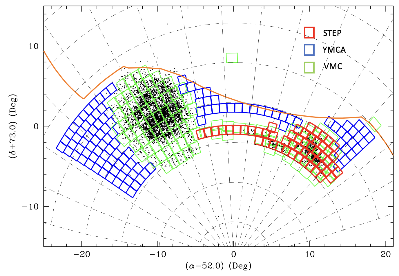
Figure 1: Footprint of the OmegaCam pointings of the YMCA survey (blue boxes) in a zenithal equidistant projection. For comparison, the footprints of the STEP (red boxes) and the VMC survey (green boxes) are also displayed in the figure. The orange solid line indicates the Southermost border of the Dark Energy Survey (DES, Dark Energy Survey Collaboration et al., 2016), which observed 5000 square degrees of the sky. Black points mark the position of all objects presented by Bica et al. (2008).

The YMCA survey has been carried out with the VLT Survey Telescope (VST, Capaccioli & Schipani, 2011), a 2.6-meter telescope located at Cerro Paranal (Chile). OmegaCam is a 32-CCD, 16k x 16k detector mosaic with a wide field of view (FoV, 1 deg², Kuijken, 2011) mounted on VST, it has a pixel scale of 0.214$\arcsec$, with thin gaps between the CCDs and an overall geometric filling factor of 91.4%. The combination of a wide field of view (FOV) and good optical quality makes OmegaCam@VST the ideal instrument to homogeneously sample the stellar components of the MCs down to the faint magnitudes required to achieve the main goals of the survey.

Figure 1 shows a footprint of YMCA in a zenithal equidistant projection along with some complementary optical and infrared surveys. As evident from the figure, most YMCA fields are centred on the LMC outer regions, while the remaining observed areas are in the north-western periphery of the SMC and in a strip in the sky linking the north-east side of the SMC with the westernmost fields of the LMC. The observations were carried out between October 2016 and December 2020, except the field 4_37 whose images were obtained in 2021 (see Table 2). We adopted the 5-point diag dithering pattern, which shifts the telescope by $\pm 25\arcsec$ and $\pm 85\arcsec$ in the X and Y direction, respectively, between two consecutive exposures. Each tile (e.g. a single OmegaCam pointing) has been observed in a “deep” mode which consists of 10 long exposures of 180 s (200 s for the fields observed in 2016-2017) and 140 s (in $g$ and $i$ filters, respectively) and in a “shallow” mode, namely 5 exposures of 25 s (both in $g$ and $i$), to avoid saturation of the brightest MC stars. When the images are stacked, we achieve an average 50% completeness level at $g\simeq 23.5-24.0$ mag (see Sect. 4.4), which is sufficient for the main goals of the survey.

Table 2 reports the essential observation log for all the 110 tiles. Figure 2 illustrates the distribution of the seeing in both filters, showing that the seeing is in the range $\sim$0.7″-1.6″and $\sim$0.7″-$\sim$1.3″, while the median is 1.13″and 0.98″, for the observations made with $g$ and $i-$filters, respectively.

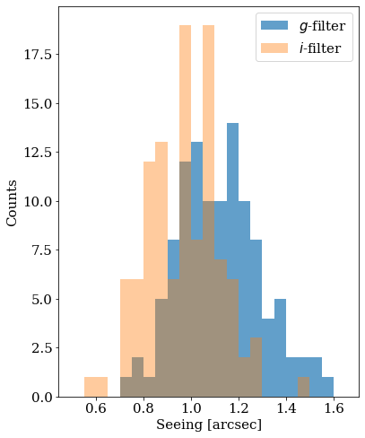
Figure 2: Histograms of the seeing, as reported in the last columns of Table 2, for observations carried out in $g$ (blue) and $i$ (red) bands.

Table 2: Log of Observations.

Tile	R.A.	Dec	Date	Sg	Si	Tile	R.A.	Dec	Date	Sg	Si
	(hms)	(dms)		(″)	(″)		(hms)	(dms)		(″)	(″)
1_27	06:23:46.392	-73:59:14.640	2016-10-11	1.24	1.01	1_28	06:38:14.976	-73:59:14.640	2016-10-12	1.34	1.00
1_29	06:52:43.584	-73:59:14.640	2016-10-12	1.51	0.96	1_30	07:07:12.192	-73:59:14.640	2016-10-23	1.30	0.87
1_31	07:21:40.776	-73:59:14.640	2016-11-19	1.34	0.82	2_30	06:41:13.272	-72:53:03.480	2017-10-12	1.30	1.06
2_31	06:54:49.056	-72:53:03.480	2017-10-13	1.17	1.17	2_32	07:08:24.864	-72:53:03.480	2017-10-12	1.30	1.01
2_33	07:22:00.672	-72:53:03.480	2016-12-18	1.05	0.73	3_1	00:06:30.648	-71:46:52.680	2018-12-12	1.23	0.85
3_10	02:01:54.576	-71:46:52.680	2018-12-15	1.15	0.88	3_21	04:22:57.144	-71:46:52.680	2017-10-12	1.09	1.09
3_32	06:43:59.688	-71:46:52.680	2020-01-04	1.16	1.07	3_33	06:56:49.032	-71:46:52.680	2020-01-04	1.03	0.80
3_34	07:09:38.352	-71:46:52.680	2020-12-13	0.92	0.86	3_35	07:22:27.672	-71:46:52.680	2020-12-14	1.03	0.81
4_1	00:06:09.144	-70:40:41.520	2018-06-07	1.24	1.09	4_2	00:18:17.256	-70:40:41.520	2018-06-08	1.28	1.08
4_9	01:43:14.040	-70:40:41.520	2018-12-14	1.24	0.83	4_10	01:55:22.152	-70:40:41.520	2018-12-15	1.09	0.98
4_11	02:07:30.264	-70:40:41.520	2018-12-15	1.01	0.88	4_12	02:19:38.376	-70:40:41.520	2018-12-17	1.17	1.09
4_13	02:31:46.488	-70:40:41.520	2018-12-17	1.06	0.80	4_14	02:43:54.600	-70:40:41.520	2019-08-21	0.98	1.06
4_15	02:56:02.712	-70:40:41.520	2019-08-22	0.89	0.90	4_16	03:08:10.824	-70:40:41.520	2019-08-23	0.90	1.08
4_17	03:20:18.936	-70:40:41.520	2019-08-22	1.07	0.98	4_18	03:32:27.048	-70:40:41.520	2019-08-22	1.04	0.97
4_19	03:44:35.160	-70:40:41.520	2017-10-12	1.19	0.98	4_20	03:56:43.272	-70:40:41.520	2017-10-13	1.13	0.99
4_21	04:08:51.384	-70:40:41.520	2017-12-23	1.08	0.97	4_22	04:20:59.496	-70:40:41.520	2017-12-25	1.12	0.99
4_33	06:34:28.728	-70:40:41.520	2020-02-22	1.23	1.09	4_34	06:46:36.840	-70:40:41.520	2020-02-12	1.02	1.08
4_35	06:58:44.952	-70:40:41.520	2020-12-15	0.96	0.77	4_36	07:10:53.064	-70:40:41.520	2020-12-16	0.92	0.82
4_37	07:23:01.176	-70:40:41.520	2021-11-26	1.6	0.74	5_1	00:05:49.992	-69:34:30.360	2018-09-16	1.48	0.93
5_2	00:17:21.312	-69:34:30.360	2018-12-13	1.54	0.87	5_3	00:28:52.656	-69:34:30.360	2018-12-13	1.37	1.05
5_21	03:56:16.680	-69:34:30.360	2018-12-12	1.38	1.07	5_22	04:07:48.024	-69:34:30.360	2017-12-26	1.13	1.08
5_23	04:19:19.368	-69:34:30.360	2018-01-11	1.25	1.09	5_36	06:49:06.720	-69:34:30.360	2020-02-27	1.05	1.17
5_37	07:00:38.040	-69:34:30.360	2020-02-27	0.93	1.04	5_38	07:12:09.384	-69:34:30.360	2020-02-29	1.46	1.13
5_39	07:23:40.728	-69:34:30.360	2020-03-02	1.44	1.14	6_1	00:05:32.832	-68:28:19.560	2017-11-20	1.13	0.87
6_2	00:16:31.176	-68:28:19.560	2017-11-20	1.12	0.90	6_3	00:27:29.496	-68:28:19.560	2018-12-14	1.26	1.11
6_4	00:38:27.816	-68:28:19.560	2018-12-14	1.10	1.06	6_5	00:49:26.136	-68:28:19.560	2018-12-14	1.16	1.07
6_6	01:00:24.480	-68:28:19.560	2018-12-15	1.09	0.93	6_23	04:06:56.040	-68:28:19.560	2018-12-12	1.19	0.90
6_24	04:17:54.360	-68:28:19.560	2018-12-13	0.99	0.81	6_37	06:40:32.616	-68:28:19.560	2020-01-04	1.22	1.27
6_38	06:51:30.960	-68:28:19.560	2020-01-03	1.31	0.97	6_39	07:02:29.280	-68:28:19.560	2020-01-03	1.00	0.95
6_40	07:13:27.600	-68:28:19.560	2020-01-03	0.87	1.16	6_41	07:24:25.944	-68:28:19.560	2020-01-02	1.12	0.86
7_1	00:05:17.400	-67:22:08.400	2017-11-23	1.27	1.02	7_2	00:15:45.960	-67:22:08.400	2017-11-20	1.33	0.96
7_3	00:26:14.496	-67:22:08.400	2017-11-20	1.27	1.25	7_4	00:36:43.056	-67:22:08.400	2017-11-23	1.37	1.13
7_26	04:27:11.160	-67:22:08.400	2018-12-12	1.14	1.10	7_27	04:37:39.720	-67:22:08.400	2018-12-14	1.45	1.11
7_38	06:32:53.784	-67:22:08.400	2020-01-03	1.22	1.08	7_39	06:43:22.320	-67:22:08.400	2020-01-01	1.23	0.98
7_40	06:53:50.880	-67:22:08.400	2020-01-01	1.14	0.97	7_41	07:04:19.416	-67:22:08.400	2020-01-01	1.04	1.50
7_42	07:14:47.976	-67:22:08.400	2020-01-02	1.38	1.06	7_43	07:25:16.536	-67:22:08.400	2020-01-02	1.03	0.95
8_1	00:05:03.456	-66:15:57.600	2017-11-22	1.30	1.18	8_2	00:15:05.016	-66:15:57.600	2017-11-22	1.40	1.02
8_3	00:25:06.576	-66:15:57.600	2017-11-28	1.20	1.21	8_28	04 35:45.696	-66:15:57.600	2018-12-15	1.20	0.89
8_39	06:26:02.880	-66:15:57.600	2020-01-01	1.22	1.03	8_40	06:36:04.464	-66:15:57.600	2020-01-03	0.95	1.11
8_41	06:46:06.024	-66:15:57.600	2019-12-31	0.96	0.76	8_42	06:56:07.584	-66:15:57.600	2019-12-31	0.92	0.71
8_43	07:06:09.144	-66:15:57.600	2019-12-31	0.86	0.88	8_44	07:16:10.704	-66:15:57.600	2019-12-31	1.02	0.96
8_45	07:26:12.288	-66:15:57.600	2020-01-01	0.94	0.93	9_40	06:19:53.976	-65:09:46.440	2019-12-29	1.17	0.99
9_41	06:29:30.984	-65:09:46.440	2019-12-30	1.00	0.93	9_42	06:39:07.992	-65:09:46.440	2019-12-31	0.76	1.08
9_43	06:48:45.000	-65:09:46.440	2019-12-29	0.97	1.00	9_44	06:58:21.984	-65:09:46.440	2019-12-30	0.92	0.79
9_45	07:07:58.992	-65:09:46.440	2019-12-30	0.84	0.82	9_46	07:17:36.000	-65:09:46.440	2019-12-30	0.98	0.83
9_47	07:27:13.008	-65:09:46.440	2019-12-30	0.90	1.00	10_42	06:23:36.600	-64:03:35.640	2018-12-17	0.75	0.62
10_43	06:32:51.168	-64:03:35.640	2018-12-17	1.01	1.16	10_44	06:42:05.736	-64:03:35.640	2019-04-10	1.06	1.18
10_45	06:51:20.304	-64:03:35.640	2019-04-10	0.97	1.03	10_46	07:00:34.872	-64:03:35.640	2019-04-11	1.20	1.14
10_47	07:09:49.440	-64:03:35.640	2019-12-29	1.16	0.85	10_48	07:19:04.008	-64:03:35.640	2019-12-29	1.08	1.00
10_49	07:28:18.576	-64:03:35.640	2019-12-29	1.08	0.81	11_41	06:00:28.848	-62:57:24.480	2017-12-09	0.98	0.96
11_42	06:09:22.848	-62:57:24.480	2018-01-08	1.15	0.77	11_43	06:18:16.848	-62:57:24.480	2018-01-14	1.05	0.72
11_44	06:27:10.848	-62:57:24.480	2018-01-19	0.93	0.85	11_45	06:36:04.872	-62:57:24.480	2018-01-19	0.97	0.82
11_46	06:44:58.872	-62:57:24.480	2018-12-12	1.02	0.87	11_47	06:53:52.872	-62:57:24.480	2018-12-13	1.20	1.26
11_48	07:02:46.872	-62:57:24.480	2018-12-14	1.20	1.27	11_49	07:11:40.896	-62:57:24.480	2018-12-15	1.16	0.74
11_50	07:20:34.896	-62:57:24.480	2018-12-16	0.96	0.71	11_51	07:29:28.896	-62:57:24.480	2018-12-16	0.80	0.59

4 Data reduction

In this section we describe the procedures adopted to i) remove the instrumental signature from the raw images; ii) obtain the astrometric calibration; iii) carry out the Point Spread Functions (PSF) photometry; iv) calibrate our photometry to the absolute system.

4.1 Pre-reduction, astrometry and PSF photometry

The pre-reduction, astrometry and stacking of all dithered images to create a single frame were performed by the VST-TUBE imaging pipeline (Grado et al., 2012, but see also the Appendix in Capaccioli et al. 2015) for all fields observed until the ESO Period 102, namely the first 21 tiles observed between October 2016 and January 2019. The VST-TUBE pipeline removes bias, performs flat-field correction, applies CCD gain equalization and applies an illumination correction. Once the pre-reduction procedure was completed, it returned two images in both the $g$ and $i$ filters, one corresponding to the stack of the “shallow” and the other to the “deep” observations. More details can be found in Grado et al. (2012) and Ripepi et al. (2014). For the remaining tiles, collected from the ESO Period 103 to 105 (April 2019-March 2020), these tasks have been performed with ASTROWISE pipeline (McFarland et al., 2013), since the VST-TUBE package was not available anymore.

Then, for all 110 YMCA tiles, we made use of the standard DAOPHOT IV/ALLSTAR (Stetson, 1987, 1992) packages to carry out the PSF photometry for each stacked shallow and deep image in both filters. To derive the PSF, we adopted an automated pipeline based on DAOPHOT IV/ALLSTAR, SExtractor (Bertin & Arnouts, 1996), and other routines written in Fortran. Once we obtained the photometry in each tile and each filter, we adopted the STILTS package (Taylor, 2006) for merging the catalogues resulting from the shallow and deep images to obtain a unique catalogue of stars in the two separate filters. Finally, we cross-matched the $g$ and $i$ catalogues to get the final photometric catalogue of each tile.

4.2 Absolute calibration

The absolute photometric calibration has been carried out employing the local standard stars provided by the “AAVSO Photometric All-Sky Survey” (APASS). For each tile, we carried out the following steps:

• We cross-matched the photometric catalogue obtained as described in Sect. 4.1 with the APASS data release 10 by adopting a search radius of 0.5″, found empirically (see Ripepi et al., 2014; Gatto et al., 2020), to mitigate the number of wrong matches (the APASS instrument’s pixel-size is 2.57″). We also retained only APASS observations with signal-to-noise (S/N) ratio larger than 10, namely with a photometric uncertainty lower than 0.1 mag.

• We searched for and corrected any residual spatial variation of the photometric zero points. To this aim, we inspected the photometric zero point difference between our photometry and the APASS one as a function of the RA and Dec.

• We corrected the colour dependence of the zero points in $g$ and $i$ filters.

At the end of this procedure, we achieved an average precision (1-sigma errors) of the order of 0.02 and 0.03 mag in $g$ and $i$ bands, respectively (see also Gatto et al., 2020). To validate our photometry we retrieved standardised synthetic photometry in the SDSS system from the Gaia Synthetic Photometry Catalogue (GSPC Gaia Collaboration et al., 2023) for about 300,000 stars in common with YMCA. The median ($\pm$ standard deviation) differences in the two passbands are $g_{\rm YMCA}-g_{\rm Gaia}=-0.011\pm 0.025$ mag e $i_{\rm YMCA}-i_{\rm Gaia}=-0.013\pm 0.024$ mag, and no perceivable colour trend, confirming that YMCA photometric zero points are very accurate.

4.3 Creation of the photometric catalogue

The final step to obtain a ready-to-use catalogue is concatenating all sub-catalogues obtained, as described in the previous sections, for each single tile. Since the dithering pattern adopted makes adjacent YMCA tiles slightly overlap at their borders, we made use of the STILTS package (Taylor, 2006) to find common stars between adjacent tiles adopting a tolerance radius of 0.25″, and get rid of duplicates. We opted for using a weighted mean of the photometry for sources in common between two or more tiles, and a simple mean for the SHARPNESS and CHI output parameters of the DAOPHOT IV/ALLSTAR (Stetson, 1987, 1992) packages. We kept in the catalogue also stars located within the overlapping regions and detected only in one tile. At the end of this procedure we obtained the final YMCA catalogue, made by 9,838,499 sources spanning 110 square degrees. Table 3 displays the first rows of the final YMCA catalogue, that provides, for each source, the coordinates, the calibrated magnitudes in both g and i filters, and finally the CHI and SHARPNESS parameters.

This catalogue still includes spurious detections due to bad pixels and extended sources. As these sources would produce undesired features in the CMD, we applied a cut using the SHARPNESS parameter. In particular, to remove also extended objects, and spurious sources near the edge of the tiles, we filtered out all sources beyond the interval -1 $\leq$ SHARPNESS $\leq$ 1. Throughout this work, any plot and/or scientific exploitation of YMCA data will refer to this point-source sub-sample made by a total of 6,467,819 stars. We also provide the scientific community with this cleaned catalogue.

Table 3: Main photometric catalogue of the YMCA survey.

RA	Dec	$g$	$\Delta_{g}$	$i$	$\Delta_{i}$	CHI	SHARP
(J2000)	(J2000)	(mag)	(mag)	(mag)	(mag)
359.92552	-72.29845	24.03	0.32	23.08	0.33	0.98	-0.34
359.92622	-72.30697	22.93	0.12	22.14	0.17	0.78	0.91
359.92649	-72.28756	23.77	0.19	22.85	0.33	0.75	0.11
359.92701	-72.28275	24.48	0.38	23.21	0.31	0.76	0.73
359.92882	-72.29437	23.88	0.19	23.31	0.38	0.70	-0.46
359.92890	-72.26670	21.98	0.08	20.30	0.04	0.98	-0.88
359.92893	-72.27306	23.90	0.29	23.04	0.28	1.03	-0.21
359.92894	-72.28692	22.94	0.10	20.46	0.05	0.78	0.20
…	…	…	…	…	…	…	…

4.4 Completeness

To derive the completeness of the survey, we followed the standard procedure by adding artificial star to the images and measuring the recovery fraction of stars as a function of magnitude. We performed this task over the entire strip defined by the tiles 7_26, 7_27, 7_38, 7_39, 7_40, 7_41, 7_42, 7_43, which surround the LMC, to probe our photometric depth at different radial distances from the LMC centre (different crowding) and/or observing conditions (e.g. seeing).

We applied the same procedure on the 8 investigated tiles. Main steps are the following: (i) Random selection of stars evenly distributed in a grid CMD with a resolution of 0.01 mag on both axes and whose intervals are: $-1.0\leq g-i\leq 3.0$ mag and $17.5\leq g\leq 26.0$ mag; (ii) Sub-division of the whole tile into boxes of 10″ per side, adding only one star per box to avoid self-crowding; (iii) PSF pipeline was carried out on the images containing the artificial stars, exactly as described in Sect. 4; (iv) Points (i), (ii), and (iii) were repeated over the same tile until the number of artificial stars was tenfold the actual number of stars detected in the tile; (v) A star was considered recovered if it is detected in both $g$ and $i$ bands, its position and magnitude estimates are within 0.25″ and 0.75 mag, respectively, from their input values, and its SHARPNESS parameter is within the same range indicated in Sect. 4.3.

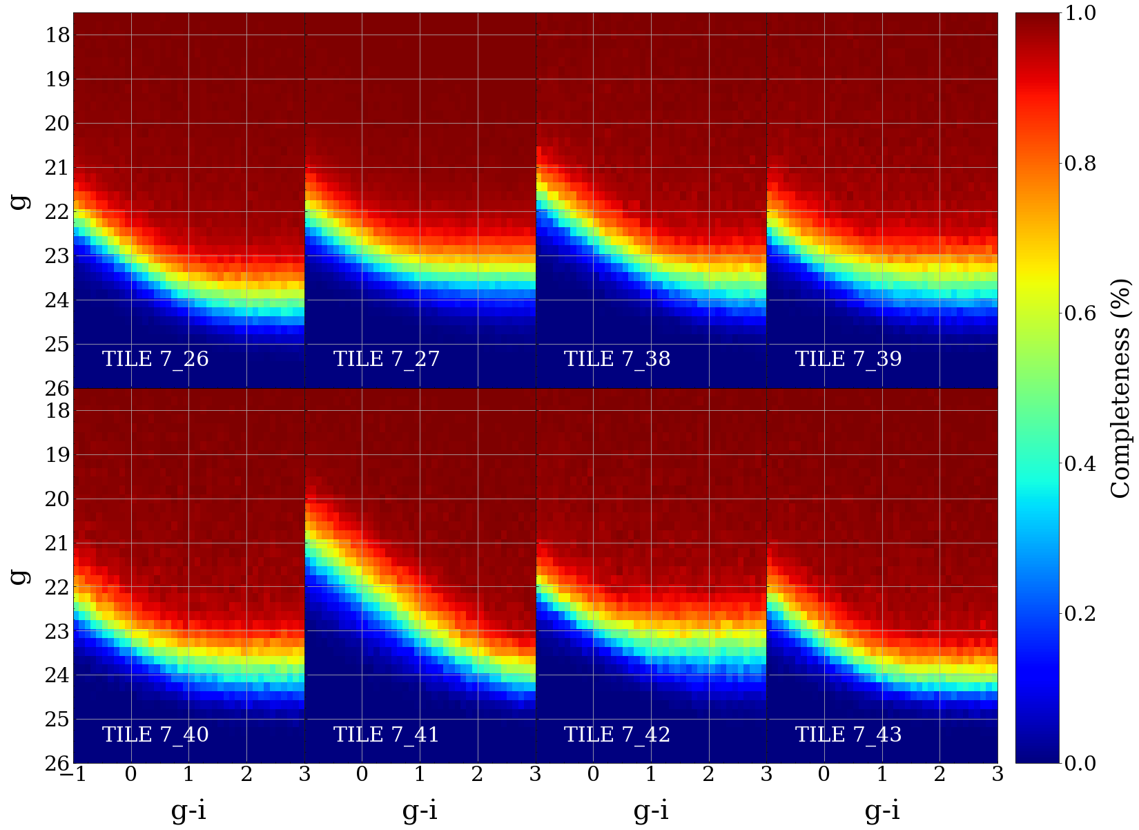
Figure 3: Completeness values in the CMD estimated in bins of 0.01 mag $\times$ 0.02 mag. Each subplot shows the measured completeness in different tiles, as indicated in the bottom left corner of each panel.

Figure 3 displays the recovery fraction of artificial stars in each bin of the CMD for the eight probed tiles. The figure shows that, if we consider the colour interval of the faint MS (e.g. $0\leq g-i\leq 1$ mag), the 50% completeness level is achieved on average between $g\simeq 23-23.5$ mag in the tiles 7_27 and 7_38 and $g\sim 23.5-24$ mag in the tiles 7_40 and 7_43. The only exception is the tile 7_41, whose 50% completeness level is reached, in the same colour intervals, at $g\simeq 22-23$ mag. We notice a strong correlation between the recovery fraction of artificial stars and the seeing (see also Table 2) rather than tiles crowding, as the tiles showing the deepest completeness levels are those with the best seeing, regardless of their distance from the LMC centre. Therefore, we assume that completeness levels for the remaining YMCA tiles might, in principle, be similar to those tiles observed in similar atmospheric conditions.

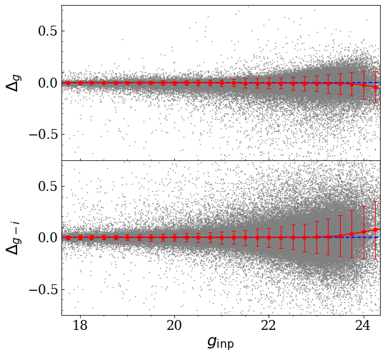
Figure 4: Magnitude difference (Top) and colour difference (Bottom), as a function of the input $g$-magnitude, between the injected and recovered artificial stars in the tile 7_26. We displayed only stars in the colour interval $0\leq g_{\rm inp}-i_{\rm inp}\leq 1$, which is typical for MC stars. Grey points show the position in these panels of each recovered artificial star, selected in the above-mentioned colour interval. Red dots and error bars indicate the mean magnitude/colour difference and their standard deviations in bins of $g_{\rm inp}$=0.25 mag.

Figure 4 shows the magnitude and colour difference between each inserted and recovered artificial star that passed the selection criteria described above in the tile 7_26, to estimate the photometric precision of the survey. Moreover, in this plot, we only included stars that had a colour input in the range $0\leq g_{\rm inp}-i_{\rm inp}\leq 1$, that embraces all MC stars in the MS, red clump (RC), and most of the RGB evolutionary phases, adopting the typical metallicities of the LMC and SMC old ($t\geq 10$ Gyr) stellar populations. The average magnitude offset for this tile measured at $g_{\rm inp}=22.5$ mag, which is the magnitude of the MSTO of the oldest stellar population of the LMC, is $\Delta_{g}=-0.01\pm 0.06$ mag, while the colour difference at the same input magnitude is $\Delta_{g-i}=0.00\pm 0.12$ mag. In particular, the standard dispersion of the magnitude and colour offsets can be used as a proxy for the statistical errors of the photometric data, and they appear to be quite small even at the faint magnitudes of the MSTO of the oldest LMC stellar population.

We examined the photometric precision also for the other seven tiles for which we performed the artificial star tests, and listed in Table 4 the average $\Delta_{g}$, and $\Delta_{g-i}$ values and their standard deviations at the $g-$magnitude of the MSTO. Most of the tiles exhibit a similar level of photometric precision, with two main exceptions, namely a higher $\delta_{g}$ within the tile 7_27 and a higher $\delta_{g-i}$ within the tile 7_41. Looking at Table 2, and at Figure 3, we speculate that the high seeing (1.45″ and 1.5″ in $g$ and $i$ for the tiles 7_27 and 7_41, respectively) may have affected the average accuracy and precision within these two tiles. Based on these considerations, we conclude that the YMCA survey achieves a precision of $\delta_{g}\sim$ 0.06 mag and $\delta_{g-i}\sim$ 0.12 mag at the MSTO magnitudes of the oldest LMC stellar population with the exceptions of tiles observed in very bad atmospheric conditions, namely with seeing higher than 1.4-1.5″. Table 4 also contains the average magnitude offset at the $g-$magnitude of the MSTO of oldest SMC stellar population, namely $g\sim$ 23 mag for each of the eight investigated tiles. The standard deviations of $\Delta_{g}\sim$ and $\Delta_{g-i}$ are only slightly larger than $g_{\rm inp}=$ 22.5 mag, despite the lower magnitude. In particular, the YMCA survey achieves a precision of $\delta_{g}\sim$ 0.08 mag and $\delta_{g-i}\sim$ 0.14 mag at the MSTO magnitudes of the oldest SMC stellar population.

Table 4: Artificial star tests.

Tile	$g_{\rm inp}$	$\Delta_{g}$	$\Delta_{g-i}$
7_26	22.5	-0.01 $\pm$ 0.06	0.00 $\pm$ 0.12
7_26	23.0	-0.01 $\pm$ 0.08	0.01 $\pm$ 0.15
7_27	22.5	0.09 $\pm$ 0.15	0.02 $\pm$ 0.21
7_27	23.0	0.12 $\pm$ 0.19	0.03 $\pm$ 0.26
7_38	22.5	0.00 $\pm$ 0.07	0.01 $\pm$ 0.16
7_38	23.0	-0.01 $\pm$ 0.08	0.04 $\pm$ 0.20
7_39	22.5	0.00 $\pm$ 0.06	0.00 $\pm$ 0.11
7_39	23.0	-0.01 $\pm$ 0.08	0.01 $\pm$ 0.14
7_40	22.5	0.00 $\pm$ 0.05	0.01 $\pm$ 0.10
7_40	23.0	0.00 $\pm$ 0.07	0.01 $\pm$ 0.13
7_41	22.5	0.00 $\pm$ 0.05	0.04 $\pm$ 0.17
7_41	23.0	0.00 $\pm$ 0.06	0.09 $\pm$ 0.24
7_42	22.5	0.00 $\pm$ 0.05	0.00 $\pm$ 0.11
7_42	23.0	0.00 $\pm$ 0.08	0.01 $\pm$ 0.15
7_43	22.5	0.00 $\pm$ 0.05	0.00 $\pm$ 0.10
7_43	23.0	0.00 $\pm$ 0.06	0.01 $\pm$ 0.14

5 Stellar populations analysis through the CMD

In this section, we describe the CMDs of the different regions surveyed by YMCA. In particular, we split the entire survey into three main sub-regions, namely the east side of the LMC, the LMC west side along the bridge that connects the two galaxies and, finally, the northwest of the SMC (see Fig. 1). All CMDs presented in this section are reddening-corrected through the reddening maps by Schlegel et al. (1998), re-calibrated by Schlafly & Finkbeiner (2011), and retrieved using the python package DUSTMAPS (Green, 2018). For the subsequent CMD analysis, throughout this work, we adopt the PARSEC suite of isochrones (Bressan et al., 2012) at varying ages and metallicities.

5.1 The east side of the LMC

Figure 5 depicts the Hess diagram of the LMC towards its eastern direction, including about 4.2 million stars located within a sky region of $\sim$67 deg². In the same figure, we also drew different isochrones spanning a range of ages from 500 Myr up to 10 Gyr, corrected for the average distance modulus of the LMC (i.e. $\rm{DM}=18.48$ mag, Pietrzyński et al., 2019).

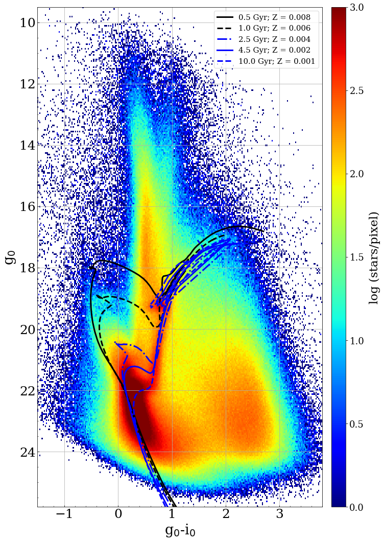
Figure 5: Hess diagram towards the eastern direction of the LMC. Each pixel is $0.02\times 0.05$ mag in size. Isochrones with different ages and metallicities, listed in the top right corner of the plot, are also superposed on the Hess diagram.

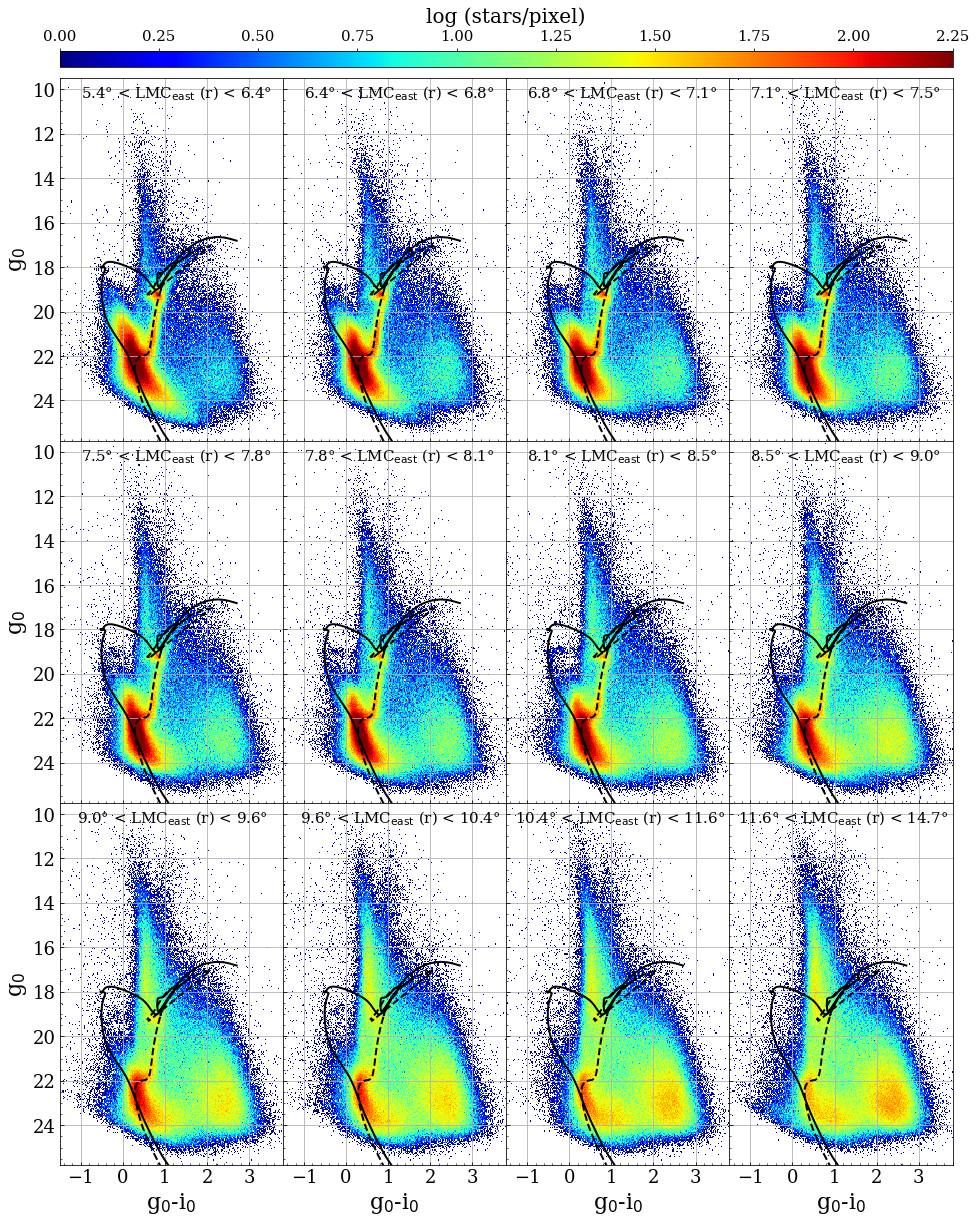
Figure 6: Hess diagrams of the LMC east side built at increasing distances from the LMC centre. Each subpanel shows about 300,000 stars. The isochrones are representative of a young and metal-richer (t = 500 Myr; Z = 0.006 dex, solid line) and old, metal-poorer (t = 10 Gyr, Z = 0.001 dex, dashed line) stellar population, corrected for the distance modulus of the LMC. At the top of each subplot, the range of angular distances from the LMC centre is indicated.

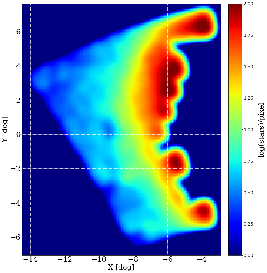
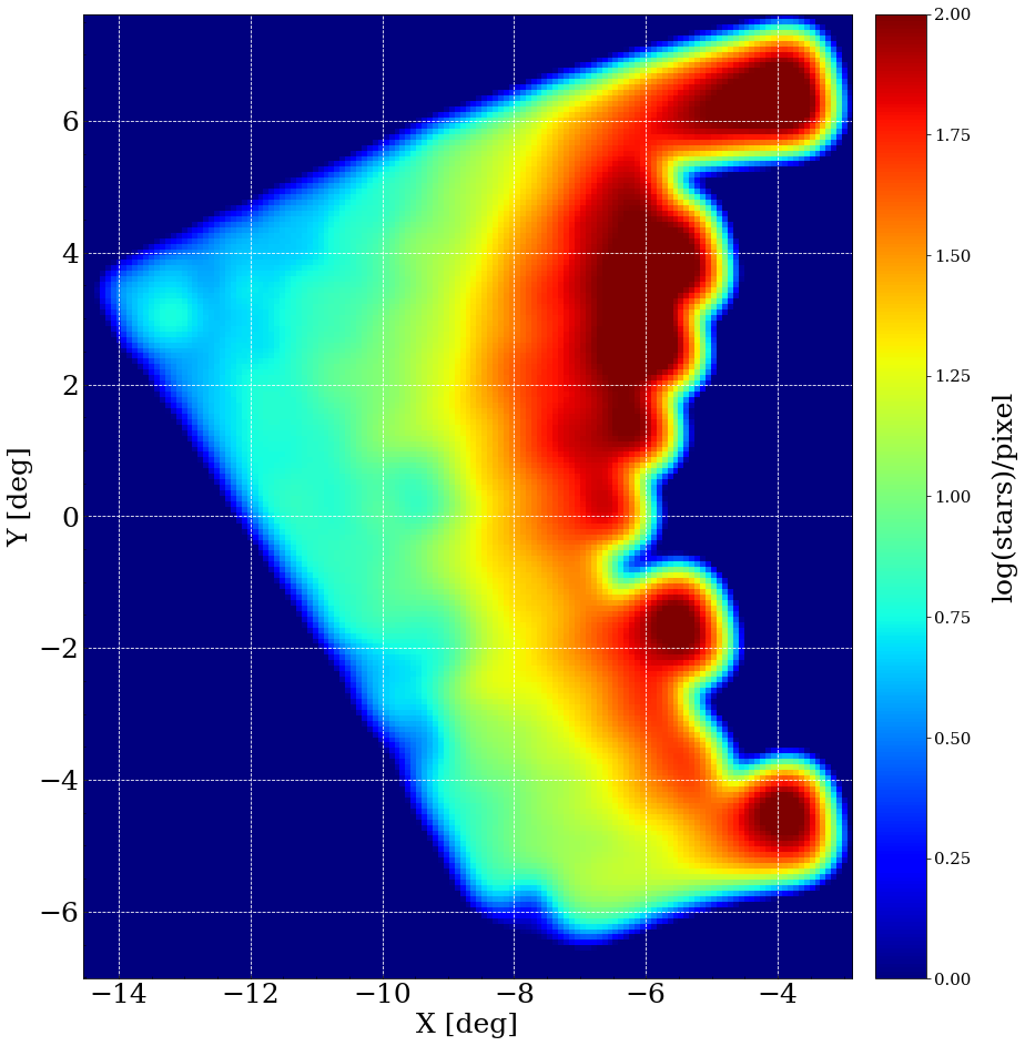
Figure 7: Density map of the LMC East periphery, constructed by adopting only MSTO stars of an intermediate-age ($7\leq t\leq 9$ Gyr, left panel) and old ($t\geq 10$ Gyr, right panel) stellar populations. Specifically, we picked up stars within the colour and magnitude range of $0\leq g-i\leq 0.5$ mag and $21.4\leq g\leq 21.9$ mag for the younger stellar population, and $0.1\leq g-i\leq 0.6$ mag and $21.9\leq g\leq 22.4$ mag, for the older one, respectively. Each pixel has size of $5\arcmin\times 5\arcmin$ and we adopted a Gaussian Kernel Density Estimator with bandwidth = 0.25° to smooth the plot.

The diagram shows that the LMC periphery is made of a mix of stars of different ages, although it is mostly dominated by intermediate-age and old stellar populations, marked by a well-defined red-giant branch (RGB) and red clump (RC). The blue plume (at $g_{0}-i_{0}\simeq-0.5$ mag and $18\leq g_{0}\leq 19$ mag) suggests the presence of a younger stellar population formed possibly about 500 Myr ago, whereas a significant recent star formation activity seems missing. Some regions of the CMD also display a severe contamination by MW foreground or halo stars. In particular, the vertical sequence at $g_{0}-i_{0}\simeq 0.6-0.8$ mag and $g_{0}\leq$19 mag, whose faint end intersects the RC evolutionary phase, is likely dominated by stars belonging to the MW thick disk, whereas the blob of stars in the Hess diagram visible between 1.5 $\leq g_{0}-i_{0}$ mag $\leq$ 3 and $g_{0}>$ 20.5 mag likely represents a mix of halo and disk MW stars (see Figure 13 in Ripepi et al., 2014, for the expected MW contamination into the CMD).

To examine the spatial distribution of the different stellar populations, Fig. 6 displays the same Hess diagram divided into 12 subplots, each one containing stars in circular annuli at increasing distances from the LMC centre; built in order to have the same number of stars (i.e. about 350,000) in each galactocentric interval. Two isochrones, representative of a young and an old stellar population are superposed onto each Hess diagram for comparison. As evident from the figure, the LMC eastern tiles cover a range of angular distances between 5.4° and about 15° (i.e. between $\sim 5$ and $\sim 13$ kpc at the LMC distance).

A close inspection of the single subplots, starting from the top left panel (i.e. the shell closest to the LMC), reveals the presence of an intermediate-age to old stellar population, as well as a relatively young one, born $\sim 0.5$ Gyr ago, traced by the blue plume. Moving towards larger distances from the LMC, the young population becomes increasingly less evident, and it disappears beyond $\simeq$9°. Therefore, the LMC old stellar population dominates the outer regions, while young stars are more concentrated at smaller distances, as already determined by previous works (e.g. El Youssoufi et al., 2021) and as usually found in star-forming dwarf and irregular galaxies (e.g., Annibali & Tosi, 2022, and references therein). Within the interval of distances between $\sim$ 7° and 10° the horizontal branch (HB) also stands out, at $-0.6\leq g_{0}-i_{0}\leq 0$ mag and $g_{0}\simeq 19.0$ mag, representing the signature of a very old population (t ¿ 10 Gyr). HB stars possibly populate also regions closer to the LMC, where, however, a clear detection is hampered by the presence of the blue plume, partially overlapping the HB. Beyond 10°, the HB is no longer detectable. At larger galactocentric distances, the contamination by MW stars becomes very high, although an old LMC stellar population is still visible also in the last distance bin (bottom right panel). These findings are in agreement with previous results (e.g. Muñoz et al., 2006; Saha et al., 2010; Nidever et al., 2019).

Note that the observed increase in background galaxies in the figure is attributed to our method of generating annuli containing an equal number of stars. Specifically, the stellar density decreases from the centre toward the outer regions. Consequently, larger areas are required to gather the same number of stars in these outer regions. Assuming a uniform density of background galaxies within the YMCA footprint (on scales larger than those of galaxy groups and clusters), this methodology leads to the inclusion of significantly more background galaxies as the area enclosed by the annuli increases.

Finally, Figure 7 presents a density map of the LMC East periphery, constructed by adopting stars within the MSTO of intermediate-age ($7\leq t\leq 9$ Gyr, left plot) and an ancient ($t\geq 10$ Gyr, right panel) stellar population. As expected, the density of stars diminishes towards the outer regions, albeit maintaining non-negligible values (especially visible in the right panel), indicating an extension of the LMC beyond the area covered by the YMCA survey in this direction (as also hinted by the bottom rightmost panel of Figure 6). Notably, the density exhibits a sudden decline at about 8° from the LMC centre, mirroring the steep drop-off in density reported by Nidever et al. (2019) in the same direction. However, a comprehensive analysis of the radial density profile of the LMC is beyond the scope of this paper.

5.2 The west side of the LMC out to the periphery of the SMC

Here we discuss the CMD of the 24 tiles located between the LMC and the SMC, approximately to the north of the classical Bridge (see Fig. 1). The westernmost tiles of this sub-sample lie in the surroundings of the LMC, whereas the easternmost ones cover the northeast periphery of the SMC. Therefore, Fig. 8, which displays the overall Hess diagram for the 1.593.456 stars within these 24 tiles, should contain a mix of LMC and SMC stars. The remarkable RGB and RC visible in this plot show that intermediate-age and old stars are still predominant, although the blue plume is more pronounced with respect to that discussed in Fig. 5, an indication of a more intense star formation activity in recent epochs in these regions.

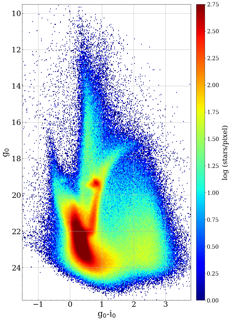
Figure 8: Hess diagram of the tiles in between the LMC and the SMC. Each pixel is $0.02\times 0.05$ mag in size. Note that to preserve the readability of the figure we do not overlap any isochrone to it as the CMD contains both LMC and SMC stars, which are therefore placed at two different distance moduli and have different metallicities.

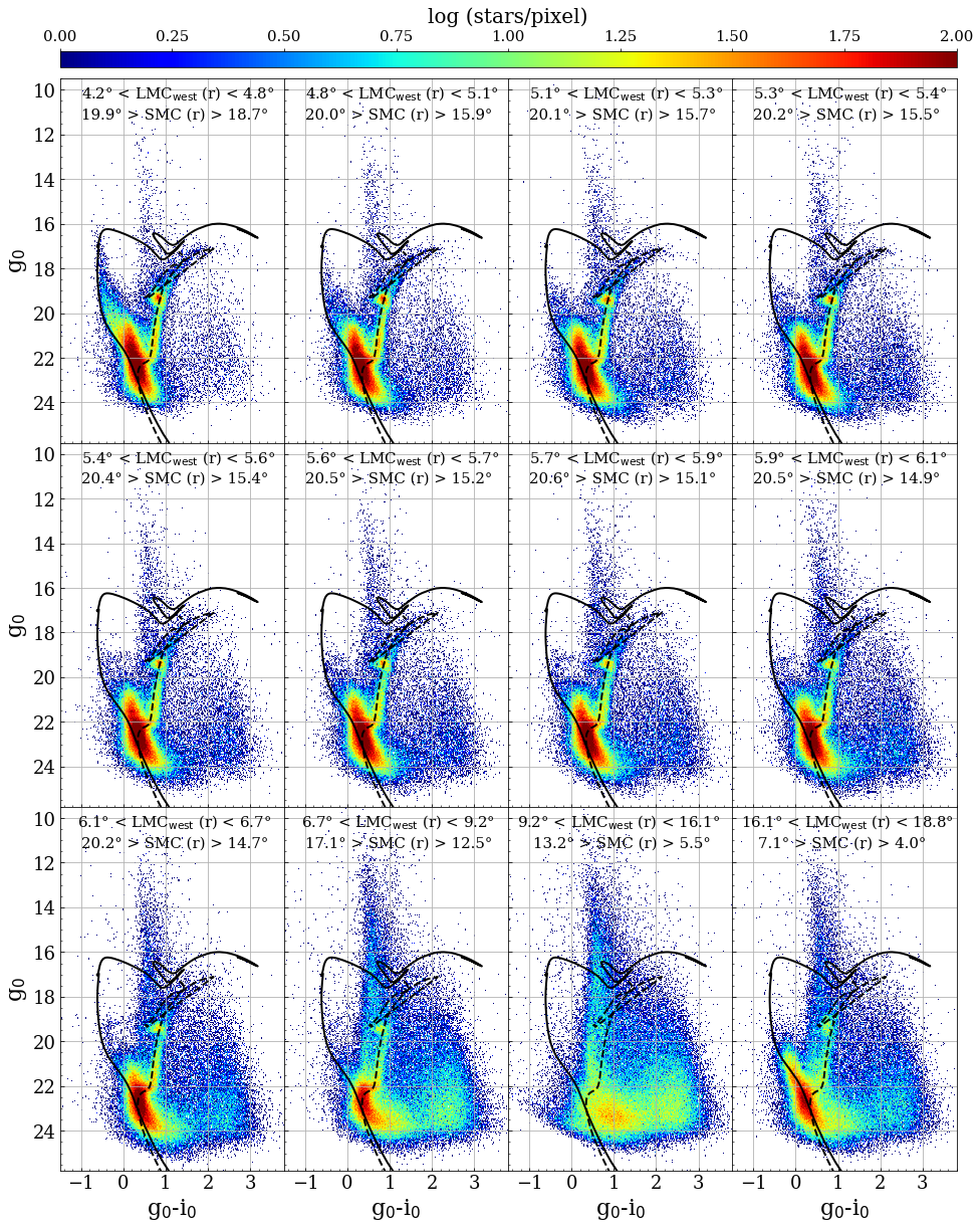
Figure 9: Hess diagrams of the tiles located between the west side of the LMC and the east side of the SMC. They are ordered based on their distance from the LMC centre. Each subpanel shows about 130.000 stars. The isochrones are representative of a young (t = 200 Myr; Z = 0.008 dex, solid line) and old (t $\sim$ 12.5 Gyr, Z = 0.001 dex, dashed line) stellar population, corrected for the distance modulus of the LMC. At the top of each subplot the range of angular distances from the LMC and SMC centres are indicated.

In Fig. 9 we show the Hess diagram of the whole region split into 12 different sub-panels, each one containing about 130.000 stars, located between $\sim 4\degr$ up to $\sim 20\degr$ from the LMC centre (the farthest layer is at about 4° from the SMC centre). Two isochrones representative of a young ($t\sim 200$ Myr; Z = 0.008) and an old ($t\sim 12.5$ Gyr; Z = 0.001) stellar population, and placed at the LMC distance, are also drawn in the figure. The top left panel, which contains the stars closest to the LMC (less than 5° from the LMC centre), exhibits the presence of stars formed about 200 Myr ago, attesting that recent events of star formation have occurred in these regions. The presence of populations younger than 200 Myr is not supported by a significant population of classical Cepheids in this tile (see Ripepi et al., 2022). All these stars belong to the easternmost part of the tile 7_27, which is spatially very close to the west rim of the LMC bar, where the northern arm of the LMC departs, regions known to host a very young stellar population (e.g. Harris & Zaritsky, 2009; Indu & Subramaniam, 2011; Gaia Collaboration et al., 2021; Mazzi et al., 2021; Ripepi et al., 2022). It is currently accepted that the intense star formation activity observed at $\sim$200 Myr is likely a consequence of the last close passage between the LMC and the SMC occurred about 150–200 Myr ago (Zivick et al., 2018, 2019; Schmidt et al., 2020; Choi et al., 2022). Stars formed about 200 Myr ago are not found beyond 5° from the LMC centre. Only intermediate-age and old stellar populations are found at larger galactocentric distances, as already observed towards the east side of the LMC. Interestingly, the density of LMC stars appears to abruptly drop down beyond $\simeq 9\degr$ ($\simeq$ 8 kpc at the LMC distance), as illustrated in the subpanel located in the third row and third column of the figure.

The density map depicted in Figure 10, constructed using MSTO stars in the strip region, provides a more detailed illustration of the sharp decline in density. Specifically, top panels show the density map of the tiles closer to the LMC, indicating that the LMC stellar population abruptly truncates at about 8°–8.5° from the LMC centre.

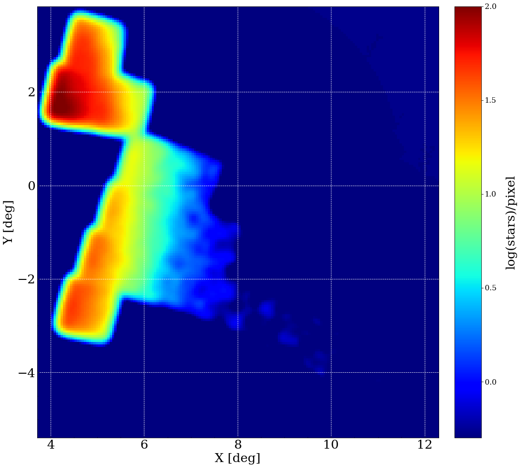
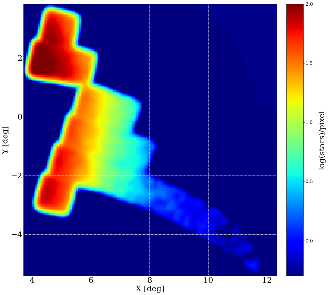
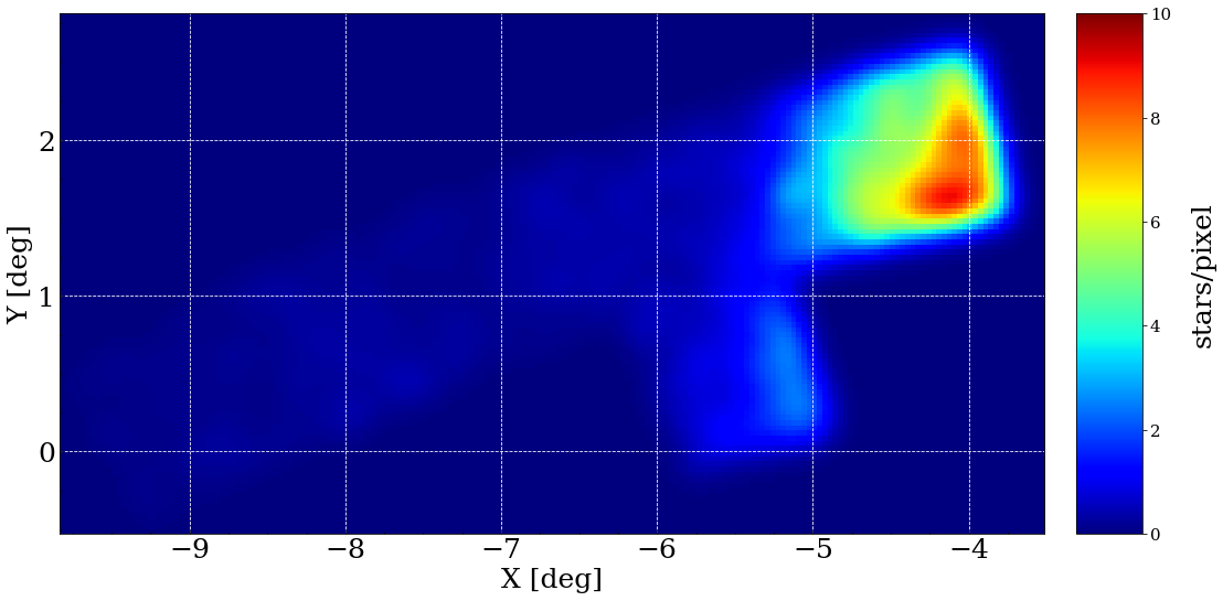
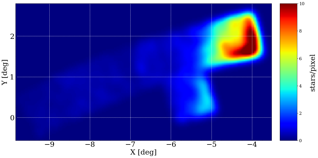
Figure 10: Top: Density map of the strip region close the LMC, derived by adopting MSTO stars corresponding to intermediate-age ($7\leq t\leq 9$ Gyr, left panel) and old ($t\geq 10$ Gyr, right panel) stellar populations. We selected stars within colour and magnitude ranges of $0.0\leq 0.5$ mag and $21.4\leq g\leq 21.9$ mag for the younger stellar population, and $0.1\leq g-i\leq 0.6$ mag and $21.9\leq g\leq 22.4$ mag, for the old one, respectively. Each pixel has size of $3\arcmin\times 3\arcmin$. Bottom: Density map of the strip region close the SMC. The region of the CMD adopted to select SMC MSTO stars is $0.0\leq g-i\leq 0.5$ mag and $21.8\leq g\leq 22.3$ mag for the younger stellar population, and $0.1\leq g-i\leq 0.6$ mag and $22.3\leq g\leq 22.8$ mag for the ancient one, respectively. Each pixel has size of $2\arcmin\times 2\arcmin$. We applied a Gaussian Kernel Density Estimator with bandwidth = 0.1° for smoothing all four subplots.

Notably, on the Eastearn side, main sequence stars of the LMC remain observable up to $\simeq 12\degr-15\degr$ (i.e. 10 - 13 kpc), as evidenced in the bottom rightmost panel of Fig. 6). This distinctive feature was previously documented by Mackey et al. (2018), who observed a sudden truncation of the LMC disc in the West and Southern regions, facing the SMC, using MSTO stars extracted from the photometric catalogue provided by the Dark Energy Survey. Furthermore, Belokurov & Erkal (2019) employed simulations to model the LMC disc’s behaviour in presence of both the MW and the SMC. Their findings suggest that a close encounter with the SMC could lead to the truncation observed on the West side of the LMC.

In the top rightmost panel, the HB begins to be perceivable and it is clearly visible when the MSTO becomes fainter than $g_{0}\simeq 20$ mag, namely beyond 5.7°. The HB stage seems to be present up to a distance of $\sim 7\degr$, then it vanishes. Interestingly, in the bottom right-central panel, with stars located between the tiles 4_12 and 4_18, that is beyond 9° from the LMC centre, the LMC stellar population is overwhelmed by MW contaminants, and an old main sequence and a feeble sub-giant branch (SGB) are only barely discernible. The last sub-panel displays the Hess diagram for stars in the North-East periphery of the SMC, in particular between $4\degr\leq r_{\rm SMC}\leq 7\degr$. It, therefore, contains SMC stars, and indeed evolutionary phases of intermediate-age and old stars are still clearly visible in the plot.

Interestingly, the magnitude of the RC, that can be used as a distance indicator (Girardi, 2016), is similar to that of the LMC.

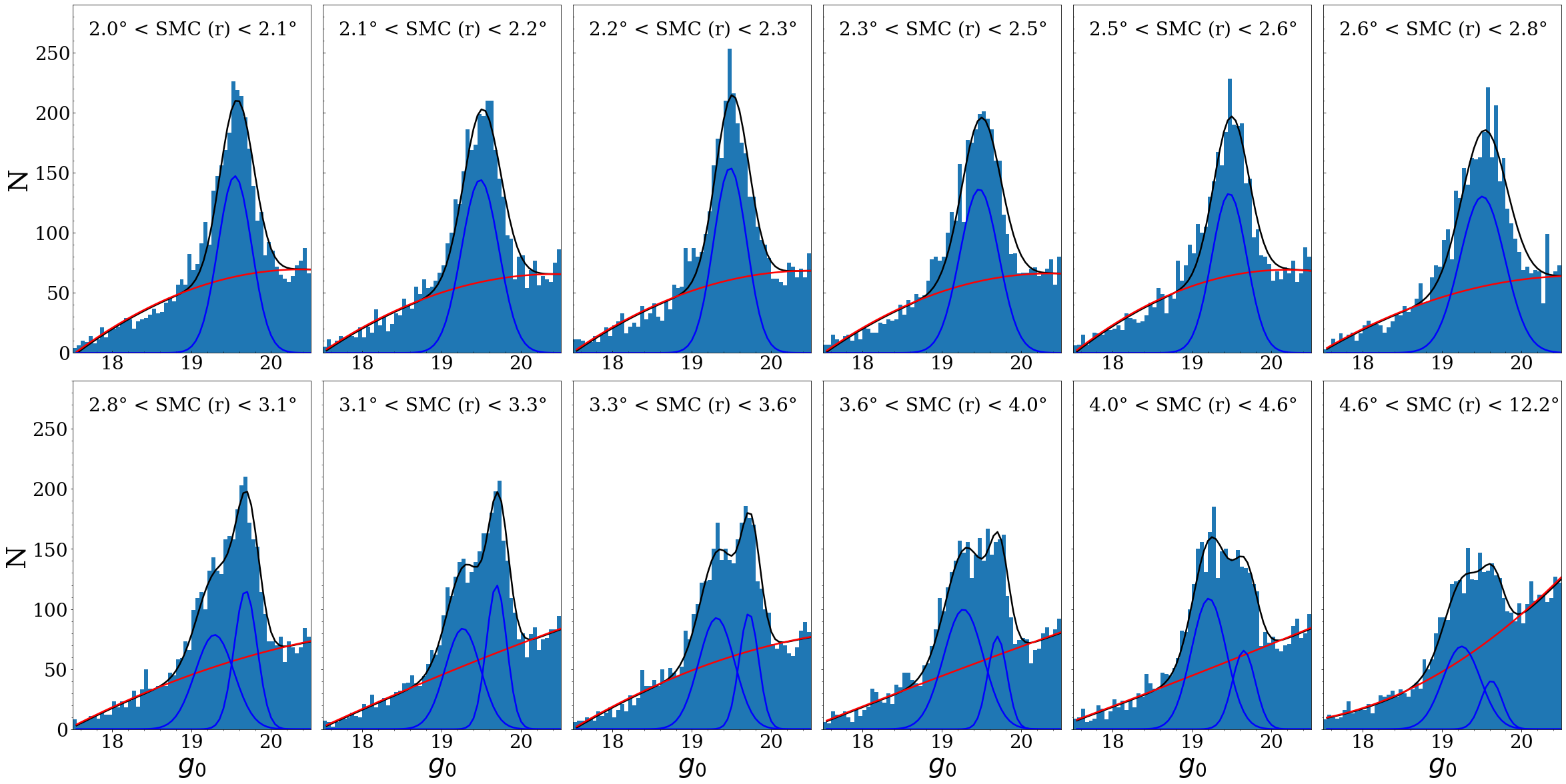
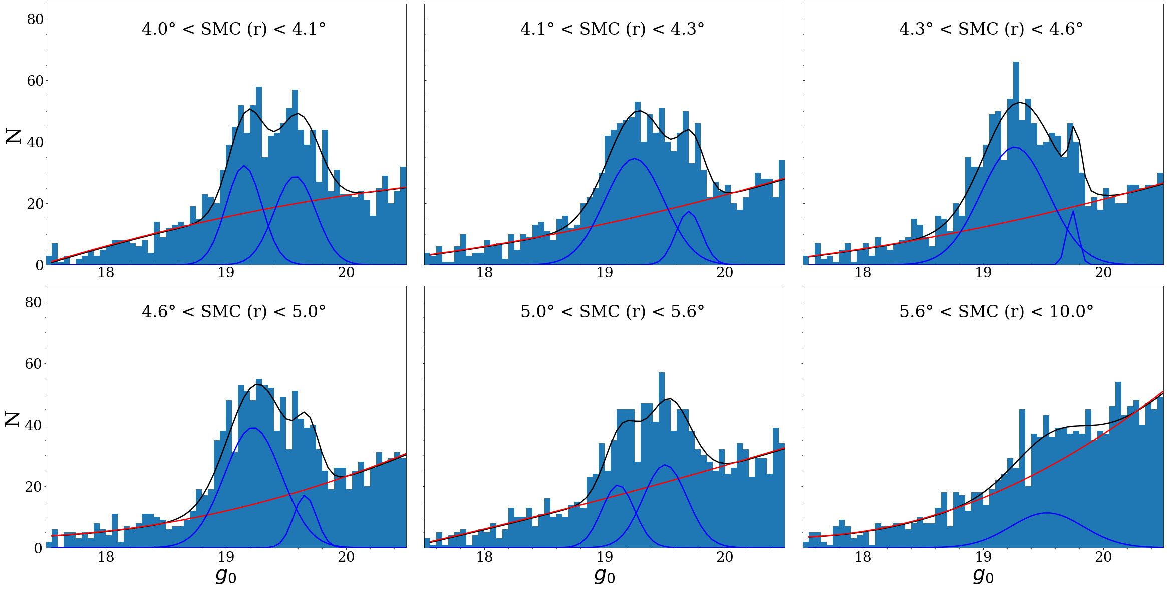
Figure 11: Magnitude distribution in the $g$ band for stars included in both the YMCA and STEP catalogues and having the position angle in the range $55\degr\leq PA\leq 95\degr$. The panels in the first two rows display $\sim$ 4360 stars with magnitudes between $g_{0}$ = 17.5 mag and $g_{0}$ = 20.5 mag, while the panels in the last two rows contain $\sim$ 1370 stars within the same range of magnitudes. At the top of each sub-panel the interval of distances from the SMC centre is reported. The blue solid lines represent the Gaussian distributions of RC stars, whereas the red solid line is the quadratic polynomial modeling the distribution of stars along the RGB. The black solid line illustrates the best-fit model derived from the combined contributions of both stellar evolutionary phases.

This might indicate that these regions are much closer to us with respect to the average distance of the SMC main body, namely $\rm DM\sim 18.9$ (de Grijs & Bono, 2015), and it could be a further consequence of the mutual gravitational interaction between the MCs. Recent works already reported the presence of a foreground SMC stellar population within SMC northeastern regions based on the analysis of the RC feature, attributing it to the tidal stripping of the LMC (Nidever et al., 2013; Subramanian et al., 2017; Tatton et al., 2021). For example, Omkumar et al. (2021) traced this substructure up to $\sim$5-6° from the SMC centre, thanks to the dataset provided by Gaia Data Release 2 (Gaia Collaboration et al., 2018), estimating that on average it is $\sim$12 kpc closer to us with respect to the SMC main body. In addition, James et al. (2021) observed in the same region a bimodal distribution in the radial velocities of RGB stars, being the two components separated by $\sim 35-45$ km s^-1. They suggested that RGB stars in the lower radial velocity component belong to the same foreground stellar substructure traced by RC stars.

In our pursuit to validate the existence of a closer SMC stellar population, we integrated the YMCA dataset with the STEP catalogue (Ripepi et al., 2014), which covers the SMC contiguously from its core to the edge of YMCA tiles. Subsequently, we conducted an analysis of the luminosity function of RC stars in the de-reddened $g$ band, following a methodology akin to that employed by Omkumar et al. (2021). Notably, the RC position in the CMD is highly contaminated by MW halo stars, as depicted in Figs. 5-8. To mitigate this, we cross-matched the YMCA+STEP catalogue with Gaia DR3, adopting a tolerance of 1″. We exclusively retained stars with reliable astrometric data characterized by RUWE ¡ 1.4 and astrometric_excess_noise_sig ¡ 2. Leveraging the Gaia dataset we excluded stars with distances and tangential velocities incongruent with those expected for the MCs. In particular, as suggested by Gaia Collaboration et al. (2021), we get rid of foreground MW stars by imposing $\bar{\omega}\leq 3\sigma_{\bar{\omega}}$, where $\bar{\omega}$ is the parallax and $\sigma_{\bar{\omega}}$ is the parallax error. Finally, we selected only stars with PMs within 5$\sigma$ from the average PM of the SMC: $0.7321-(5\cdot 0.3728)\leq\mu_{\alpha}\leq 0.7321+(5\cdot 0.3728)$ and $-1.2256-(5\cdot 0.2992)\leq\mu_{\delta}\leq-1.2256+(5\cdot 0.2992)$. These average SMC PM values and their associated uncertainties were derived from Gaia Collaboration et al. (2021).

Following Girardi & Salaris (2001) we modeled the magnitude distribution of $g_{0}$ adopting the following equation:

$$N(g_{0})=a+b\cdot g_{0}+c\cdot g_{0}^{2}+d\cdot{\rm exp[-\frac{(g_{0}-g_{0}^{\rm RC})^{2}}{2\sigma_{g_{0}^{2}}}]}$$ (1)

where the Gaussian function models the RC distribution, while the quadratic polynomial accounts for RGB stars contaminants. Additionally, we introduced the possibility of including a second Gaussian function to assess the potential presence of a foreground stellar population within the SMC. We sub-divided the YMCA-STEP catalogue into slices at different angular distances from the SMC centre, each holding an equal number of stars, in the direction of the observed closer RC stellar population. Specifically, we confined our analysis to stars falling within the position angle range: $55\degr\leq PA\leq 95\degr$. Employing the LMFIT Python package, we conducted individual fits within each slice, considering a model with two Gaussians only when their centres were separated by at least the sum of their widths.

Figure 11 illustrates the results obtained from the fit of regions at increasing angular distances, moving from the top left to the bottom right. The top two rows correspond to distances ranging between $2.0\degr$ and $12.2\degree$, with approximately 4360 stars in each sub-panel. The last two rows, that aim to better visualize the outer regions that contain less stars, encompass distances between 4° and 10°, with approximately 1370 stars in each sub-panel. Our analysis reveals a discernible foreground stellar population emerging around $\sim 2.8\degree$ from the SMC centre, becoming more prominent at greater angular distances and becoming the predominant feature beyond $\simeq 3.5\degr$. However, beyond 5.0°, the faint RC appears again as the dominant stellar population, and beyond $\simeq 5.5\degree$, the foreground stellar population becomes indiscernible. Table 5 provides the mean and standard deviation of the Gaussians for each slice, indicating that the closer stellar population exhibits an average distance modulus smaller than 0.4 mag, corresponding to about 14.5 kpc at the distance of the SMC. These findings align with the conclusions drawn by Omkumar et al. (2021).

Table 5: Statistics of the Gaussian approximating the RC stellar population within the investigated region.

r	$g_{0}^{\rm RC_{f}}$	$g_{0}^{\rm RC}$
2.0°- 2.1°	-	19.5 $\pm$ 0.2
2.1°- 2.2°	-	19.5 $\pm$ 0.2
2.2°- 2.3°	-	19.5 $\pm$ 0.2
2.3°- 2.5°	-	19.5 $\pm$ 0.2
2.5°- 2.6°	-	19.5 $\pm$ 0.2
2.6°- 2.8°	-	19.5 $\pm$ 0.3
2.8°- 3.1°	19.3 $\pm$ 0.2	19.7 $\pm$ 0.1
3.1°- 3.3°	19.3 $\pm$ 0.2	19.7 $\pm$ 0.1
3.3°- 3.6°	19.3 $\pm$ 0.2	19.7 $\pm$ 0.1
3.6°- 4.0°	19.3 $\pm$ 0.2	19.7 $\pm$ 0.1
4.0°- 4.6°	19.2 $\pm$ 0.2	19.7 $\pm$ 0.1
4.6°- 12.2°	19.2 $\pm$ 0.2	19.6 $\pm$ 0.1
4.0°- 4.1°	19.2 $\pm$ 0.1	19.6 $\pm$ 0.2
4.1°- 4.3°	19.2 $\pm$ 0.2	19.7 $\pm$ 0.1
4.3°- 4.6°	19.3 $\pm$ 0.3	19.7 $\pm$ 0.0
4.6°- 5.0°	19.2 $\pm$ 0.2	19.7 $\pm$ 0.1
5.0°- 5.6°	19.1 $\pm$ 0.1	19.5 $\pm$ 0.2
5.6°- 10.0°	-	19.5 $\pm$ 0.3

5.3 The unexplored north-west periphery of the SMC

In this section, we discuss the characteristics of the $\sim$700,000 stars placed in the 19 tiles on the northwestern side of the SMC. As in the previous sections, Fig. 12 shows the overall Hess diagram of all stars in these fields, along with three isochrones of different ages, corrected for the distance modulus of the SMC (${\rm DM}=18.9$ mag). Unlike the regions previously described, the absence of the blue plume in the plot denotes the absence of any population younger than $\simeq 1.0$ Gyr, while the RC and RGB evolutionary phases are evident, indicating that the periphery of the SMC is made only by intermediate-age and old stars.

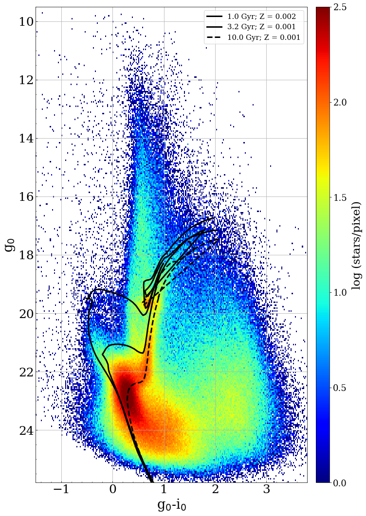
Figure 12: Hess diagram of the 19 tiles centred at the north-western periphery of the SMC. Each pixel is $0.02\times 0.05$ mag in size. Three different isochrones, with ${\rm DM}=18.9$ mag and ages and metallicities listed in the top right corner of the plot, are also superposed on the Hess diagram.

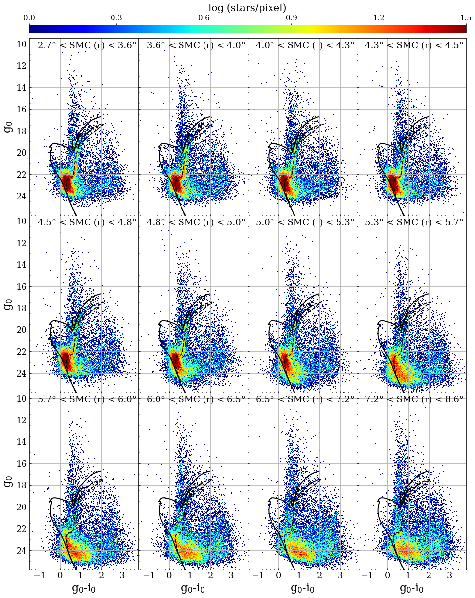
Figure 13: Hess diagrams of the fields on the northwest side of the SMC. Each subpanel contains about 60.000 stars, and they are ordered according to their distance from the SMC centre. Two isochrones (t = 1 Gyr; Z = 0.001 dex, solid line and t = 10 Gyr, Z = 0.001 dex, dashed line), corrected for the distance modulus of the SMC, are superposed as a comparison. At the top of each subplot the range of distances from the SMC centre is indicated.

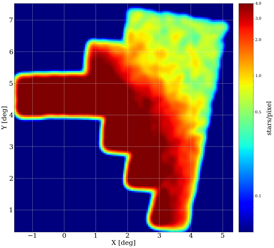
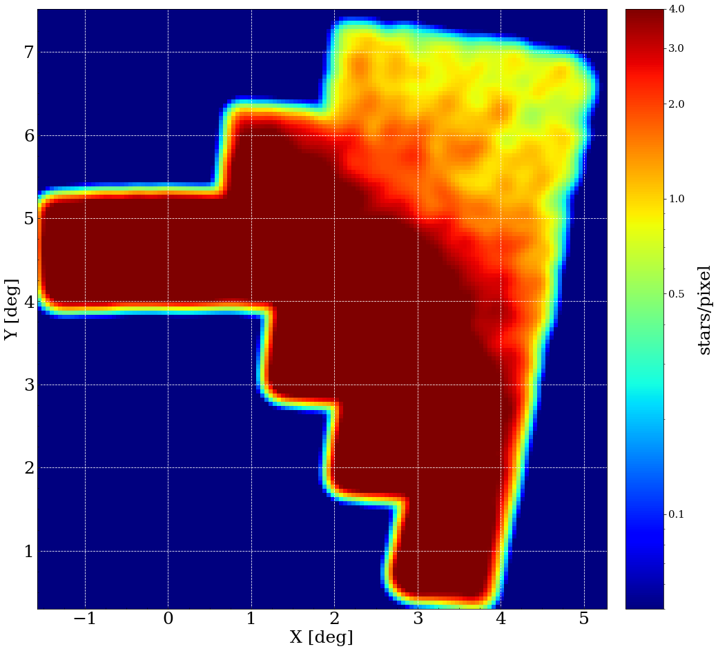
Figure 14: Density map of the SMC north-western periphery, derived by adopting MSTO stars corresponding to intermediate-age ($7\leq t\leq 9$ Gyr, left panel) and old ($t\geq 10$ Gyr, right panel) stellar populations. Specifically, we selected stars within colour and magnitude ranges of $0.0\leq g-i\leq 0.5$ mag and $21.8\leq g\leq 22.3$ mag for the left panel, and $0.1\leq g-i\leq 0.6$ mag and $22.3\leq g\leq 22.8$ mag for the right panel, respectively. Each pixel has size of $3\arcmin\times 3\arcmin$ and we applied a Gaussian Kernel Density Estimator with bandwidth = 0.1° for smoothing the plot.

To analyze the trend of the stellar population with the distance from the SMC centre, in Fig. 13, we display 12 Hess diagrams for stars at different galactocentric radii. Each subplot contains about 60,000 stars and we also draw two isochrones of 1 Gyr and 10 Gyr to guide the eye. These tiles cover an interval of galactocentric distances between $\sim$ 3° and 8.5° , corresponding to $\sim$ 3 and $\sim$ 9 kpc at the mean distance of the SMC. The shell closest to the SMC reveals that the youngest stellar population in this area is possibly older than 1 Gyr, suggesting a total absence of recent star formation in the northwest side of the SMC. On the contrary, it is known that the SMC main body and its eastern direction (i.e. the Wing) underwent a very intense recent period of star formation (Cignoni et al., 2013; Rubele et al., 2018). The intermediate-age and old stellar population coexist up to $\sim$5.7°, beyond which the RGB and RC begin to fade. In the farthest two subpanels the densest areas of the Hess diagram are at $g_{0}-i_{0}\sim 1$ mag and $g_{0}\sim 24$ mag, which likely represent MW halo stars (see also Fig. 13 in Ripepi et al., 2014). In all these plots the HB is less evident with respect to what was observed in the outskirts of the LMC (see Figures 6 and 9), a clue that the star formation activity at look-back times greater than 10 Gyr was not so energetic as in the LMC (Cignoni et al., 2013). Many authors reported a substantial difference in the SFHs of the MCs for the period between 10 Gyr and 12-13 Gyr, casting doubt on them having formed as a pair (see e.g. Rezaeikh et al., 2014; Massana et al., 2022, and references therein).

Figure 14 displays the density map of the SMC north-western periphery, as traced by MSTO stars belonging to intermediate-age ($7\leq t\leq 9$ Gyr, left plot) and ancient ($t\geq 10$ Gyr, right panel) stellar populations. Unlike the LMC, at a radial distance of about 6°, corresponding to 6.3 kpc, the density of the younger population sharply approaches zero, suggesting the border of the SMC in this direction. This feature can also be hinted at by looking in subplots of Figure 13 displaying radial distances greater than $\sim$6.5°.

6 Discovery of unknown star clusters in the MC periphery

In Gatto et al. (2020), we presented a list of 78 new candidate SCs, which were discovered in the outskirts of the LMC using an algorithm designed to identify over-densities characteristic of SCs in the sky. That work was based on 21 YMCA + 2 STEP tiles in the vicinity of the LMC available at that time. Here we report the results of the cluster-finding algorithm applied to the remaining 79 YMCA tiles, including those located in the periphery of the SMC and in the region between the LMC and SMC.

6.1 Main steps of the cluster finding algorithm

The working flow of the algorithm is thoroughly described in Sect. 3 of Gatto et al. (2020). Here, we provide a brief summary of the process. The algorithm takes the coordinates of stars as its only input parameter, and processes each tile individually to identify regions of the sky where the number of stars is higher than the local background. To achieve this, it performs a Kernel Density Estimation (KDE) on each tile using both the tophat and the gaussian functions as kernels, with a bandwidth of 0.2′. The algorithm then automatically determines the centres and radii of the detected over-densities (see Sect. 3.2 of Gatto et al., 2020). The final outcome is a list of over-densities for each tile, including some that are not actual physical systems (usually called asterisms) and must be removed, as described in the next Section.

6.2 Cleaning the colour-magnitude diagram from field star contamination

To distinguish between real SCs and asterisms we first have to decontaminate the CMD of the SC candidates from field stars. Following Gatto et al. (2020), we adopt the method described by Piatti & Bica (2012) to clean the CMDs, which is well-suited for sparse SCs, such as those found in this work. In this paper, we apply a method slightly different from that adopted in Gatto et al. (2020); therefore, we summarize the method below. In this procedure, the CMD of each SC candidate (over-density) is compared with those of six surrounding fields with the aim to identify probable field stars and remove them from the SC CMD. Each field is defined as a circular region with a radius three times that of the SC candidate, thereby ensuring a sufficient sample size of the local stellar background even in low-density environments. For each of the six fields, boxes centred on each star are constructed, with sides that vary based on the local density of the CMD stars. In particular, small boxes are constructed in denser areas (see Fig. 12 in Piatti & Bica, 2012, for an example of the procedure). Note that in the following steps we leave out stars within the CMD region defined by $g-i>1.5$ mag and $g>20$ mag, as these are likely MW dwarf disk stars (see Fig. 13 in Ripepi et al., 2014) that could alter the outcome of the cleaning procedure.

The median number of stars in the six fields is estimated and normalized to the SC area, providing an estimate of the expected number of contaminant stars ($N_{\rm bkg}$) in the SC area. Subsequently, in order to determine the likelihood of a star belonging to the candidate SC, we randomly extracted $N_{\rm bkg}$ stars for each field, and then identified and subtracted the $N_{\rm bkg}$ closest stars in the CMD of the candidate SC for each of the six surrounding fields. This process was repeated for all six fields and the probability of a star belonging to the cluster was calculated as $P=1-(N_{\rm subt})/6$, where $N_{\rm subt}$ refers to the number of times a star was subtracted. The position of the stars with a high membership probability on the CMD was then utilized to distinguish between real physical systems and asterisms, and to estimate the age of the SCs through an isochrone fitting procedure (see Sect. 6.3).

As done in Gatto et al. (2020), to quantitatively gauge the goodness of each SC we also estimate the number of stars hosted by the SC divided by the standard deviation above the local average mean. Hence, we define

$$G=(N_{\rm cl}-N_{\rm bkg})/\sqrt{N_{\rm bkg}}$$ (2)

where $N_{\rm cl}$ is the number of stars within the SC radius. With respect to Gatto et al. (2020), we preferred a more conservative approach by taking into consideration only candidate SCs with $G>5.0$. The CMDs of the SC passing this selection were subsequently analysed in more detail as explained in the following section.

6.3 Determine SC age through isochrone fitting

To determine the age of each SC candidate, we adopted a visual isochrone matching procedure. The PARSEC isochrones by Bressan et al. (2012) were used and the distance modulus was fixed to either ${\rm DM}=18.49$ mag or ${\rm DM}=18.9$ mag for SCs located in the LMC and SMC peripheries, respectively. The metal content was fixed based on the age-metallicity relation derived by Piatti & Geisler (2013) and Parisi et al. (2015) for the LMC and SMC, respectively. We varied the age of the isochrones to seek the best one that matches the positions of the stars with high membership values (i.e. $P\geq 50\%$) on the de-reddened CMD. In particular, we focus on the following evolutionary phases to aid the matching procedure: MS, RC, RGB, and sub-giant branch (SGB). To be conservative, we considered an age uncertainty of $\sigma_{\log t}=0.2$ dex, which includes both the statistical error from the visual procedure and the systematic error due to the elongation of the LMC/SMC along the line of sight. To assess the accuracy of the SC ages estimated via this procedure, we provide a comprehensive comparison of our SC ages with those in common with the existing literature in Appendix A.

6.4 Candidate SCs in the MC periphery

Table 6: Main parameters of the SCs investigated in this work.

ID*	RA	Dec	R	$\log t$	${\rm N_{\rm stars}}$	G	$n_{0}$	$r_{c}$	$r_{c}$	Tile	Flag	Simbad Name
	(J2000)	(J2000)	(’)				(arcmin-2)	(’)	(pc)
YMCA-0049	11.8554	-68.9199	1.10	9.60	422	47.7	$676\pm 7$	$0.32\pm 0.13$	$5.6\pm 2.2$	6_5	A	L 32; OGLE-CL SMC 310
YMCA-0050	14.7444	-68.9153	0.85	9.70	210	31.6	$382\pm 5$	$0.28\pm 0.03$	$4.8\pm 0.5$	6_6	A	ESO 51-9; OGLE-CL SMC 309
YMCA-0051	25.4233	-71.1624	0.70	9.20	165	22.9	$249\pm 8$	$0.34\pm 0.19$	$5.0\pm 2.7$	4_9	A	HW 84; OGLE-CL SMC 305
YMCA-0052	28.2998	-70.7526	0.95	9.85	79	14.0	$187\pm 9$	$0.14\pm 0.02$	$2.0\pm 0.4$	4_10	A	OGLE-CL MBR 6
YMCA-0053	66.7160	-67.2567	0.50	9.75	54	6.6	$83\pm 9$	$0.24\pm 0.12$	$3.5\pm 1.7$	7_26	B
YMCA-0054	67.3571	-67.4461	0.40	9.40	62	6.9	$337\pm 10$	$0.14\pm 0.05$	$2.0\pm 0.7$	7_26	A	OGLE-CL LMC 0841
YMCA-0055	67.6149	-67.7673	0.25	9.45	27	5.2	$136\pm 17$	$0.16\pm 0.12$	$2.4\pm 1.7$	7_26	C
YMCA-0056	67.6596	-66.9542	0.35	9.25	77	15.7	$486\pm 10$	$0.16\pm 0.05$	$2.3\pm 0.7$	7_26	A	HS 8; KMHK 5
YMCA-0057	67.8233	-67.7799	0.20	9.40	22	5.5	$228\pm 16$	$0.12\pm 0.10$	$1.8\pm 1.4$	7_26	C	OGLE-CL LMC 0834
YMCA-0058	68.8670	-67.7115	0.50	9.30	112	9.2	$284\pm 10$	$0.17\pm 0.02$	$2.5\pm 0.3$	7_27	A	HS 13; KMHK 11
YMCA-0059	69.4153	-66.1983	1.30	9.25	836	33.8	$692\pm 25$	$0.38\pm 0.06$	$5.5\pm 0.9$	8_28	A	ESO 84-30; LW 11; NGC 1644; SL 9
YMCA-0060	69.7900	-67.4985	0.25	9.40	38	5.9	$164\pm 14$	$0.19\pm 0.06$	$2.8\pm 0.9$	7_27	C
YMCA-0061	69.9930	-67.3831	0.35	9.80	62	6.0	$176\pm 21$	$0.21\pm 0.13$	$3.1\pm 1.9$	7_27	C
YMCA-0062	93.9911	-64.9733	0.60	9.25	178	17.0	$615\pm 19$	$0.19\pm 0.06$	$2.7\pm 0.8$	9_40	A	KMHK 1710; LW 444
YMCA-0063	94.4250	-65.5469	0.40	9.45	86	11.2	$456\pm 9$	$0.15\pm 0.02$	$2.1\pm 0.3$	9_40	A	OGLE-CL LMC 0758
YMCA-0064	94.4670	-65.3440	0.30	9.45	33	5.0	$85\pm 8$	$0.21\pm 0.16$	$3.1\pm 2.4$	9_40	C
YMCA-0065	96.1209	-66.5061	0.45	9.20	109	13.7	$448\pm 18$	$0.18\pm 0.05$	$2.7\pm 0.7$	8_39	A	OHSC 34; KMHK 1751
YMCA-0066	96.2493	-66.5821	0.40	9.40	58	6.6	$235\pm 14$	$0.12\pm 0.02$	$1.8\pm 0.4$	8_39	B
YMCA-0067	97.0305	-67.2605	0.35	9.35	35	6.2	$139\pm 6$	$0.18\pm 0.07$	$2.7\pm 1.1$	7_38	B
YMCA-0068	97.4257	-70.5889	0.80	9.25	226	13.4	$309\pm 12$	$0.25\pm 0.04$	$3.6\pm 0.6$	4_33	A	OHSC 36; KMHK 1757
YMCA-0069	97.4821	-70.4781	0.35	9.45	39	6.1	$124\pm 6$	$0.19\pm 0.15$	$2.8\pm 2.1$	4_33	C
YMCA-0070	97.5571	-64.3277	2.50	10.10	3291	227.8	$1013\pm 10$	$0.74\pm 0.05$	$10.8\pm 0.8$	10_43	A	ESO 87-24; KMHK 1756; LW 481;
												NGC 2257 ; SL 895
YMCA-0071	98.0190	-70.5724	0.40	9.35	42	5.0	$176\pm 12$	$0.11\pm 0.02$	$1.7\pm 0.4$	4_33	B
YMCA-0072	98.2564	-71.1269	1.00	9.00	417	32.8	$377\pm 7$	$0.43\pm 0.11$	$6.3\pm 1.5$	4_33	A	KMHK 1760; LW 483; SL 897
YMCA-0073	106.9160	-69.9839	0.50	9.75	51	23.9	$355\pm 8$	$0.16\pm 0.06$	$2.3\pm 0.9$	5_38	A	KMHK 1762; OHSC 37

Table 6 lists the main parameters of the 25 SCs identified within the 79 remaining YMCA tiles. Within these regions, sixteen of them were already reported in the literature, while the remaining nine are new discoveries. As a result, we have increased the number of previously known SCs in these fields by $\simeq 50\%$.

It is important to note that we did not find any new SC within the YMCA tiles located in the periphery of the SMC, and therefore all the 9 newly detected candidate SCs reside in the outskirts of the LMC. Among the main SC parameters, the table provides the G value defined in the Eq. 2 and a flag assigned subjectively to each SC to classify them as likely real physical systems versus possible asterisms. Our assessment of each SC is based on its statistical significance, such as the ${\rm G}$ parameter, or the discernible presence in the CMD of distinct evolutionary phases, such as the RC or a well-defined RGB. Additionally, Figures 18 and 20 illustrate the CMDs of all the SCs studied in this work.

Figure 15 illustrates the relative spatial position of the 21 SCs located in the LMC periphery, with respect to the centre of the LMC itself. The majority of the SCs detected in this work are located in close proximity to those previously known. In particular, all newly discovered SCs reside within 7° from the LMC centre, consistent with previous findings (Pieres et al., 2016; Gatto et al., 2020), in spite of the fact that the LMC disc extension is significantly larger (e.g. Saha et al., 2010). Note that this result is not due to an observational bias, as the YMCA tiles used in this work cover regions of the LMC up to $\sim$15° from its centre. The same Fig. 15 suggests the presence of a possible SC clump at ($\xi$, $\eta$) $\simeq$ (5°,-2°), corresponding to the tiles $7\_26-7\_27-8\_28$. These tiles are amongst the ones with the highest number of stars and the closest to the LMC centre. Consequently, in principle, it may be hypothesized that the SC over-density in this region is a result of the highest number of stars located in these tiles. However, this hypothesis is challenged by the observation of a low number of SCs in tiles with a similar number of stars (e.g. tile $8\_39-9\_40$) or by the complete absence of SCs in tiles at similar radial distances (e.g. tile $6\_24$). As the SC agglomeration is located at the edge of the LMC bar, a more plausible explanation may be a higher level of star formation occurred in this region in the last Gyrs (Mazzi et al., 2021).

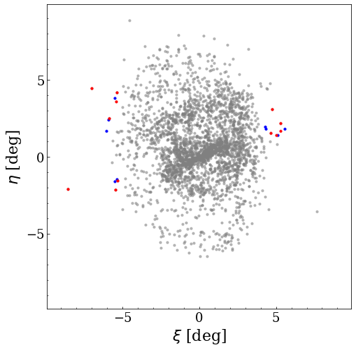
Figure 15: Relative positions of the 21 SCs located in the surroundings of the LMC, with respect to the LMC centre. Coloured points indicate the clusters identified in this work, in red those already known in the literature, in blue the newly discovered ones. Grey points represent SCs reported in the catalogue by Bica et al. (2008).

6.5 The age distribution of the SCs in the LMC outskirts

Figure 16 shows the age distribution of the 21 candidate SCs in the LMC outskirts, as well as of 10 SCs reported in Gatto et al. (2020) with $G\geq$ 5. The distribution exhibits a prominent peak at approximately 2.0-3.0 Gyr, which is consistent with the findings of Gatto et al. (2020). The number of SCs steadily decreases towards younger ages ($t\leq 2$ Gyr), while on the opposite side, after 3 Gyr, namely slightly before the beginning of the period dubbed as the age gap, it sharply drops down. The sudden SC formation enhancement at $\sim 3.0$ Gyr may be associated with a past close encounter between the MCs, which triggered a new episode of massive SC formation. This is independently supported by different works that tried to reconstruct the history of the orbital path of the MCs, and most of them agree that a past pericentric passage between the LMC and SMC happened between 1 and 3 Gyr ago (see for example, Bekki & Chiba, 2005; Patel et al., 2020, and references therein). Interestingly, Pieres et al. (2016) reported a similar peak at $\sim$ 2.7 Gyr by analysing the CMD of 109 SCs to the Northern side of the LMC. However, they also evidenced a major peak at $\sim$ 1.2 Gyr that is not present in our SC sample. Indeed, we detected only two SCs younger than 1.5 Gyrs and none of them is younger than 1 Gyr, suggesting that no recent SC formation event occurred in the LMC outskirts, at least in our analyzed tiles. The lack of young SCs (younger than 1 Gyr) in our sample is consistent with the general consensus that the periphery of the LMC is inhabited by an old population (Saha et al., 2010; Piatti & Geisler, 2013; Mazzi et al., 2021).

Alternatively, these results may indicate that an episodic increase in the SC formation $\sim 1-2$ Gyrs ago occurred in the Northern region of the LMC, investigated by Pieres et al. (2016), leaving quite unaltered the fields investigated in this work. To explore this possibility, we took advantage of Mazzi et al. (2021)’s work that derived the spatial-resolved SFH of the LMC in 96 deg², down to sub-spatial regions of 0.125 deg², using near-infrared observations from the VMC (Cioni et al., 2011).

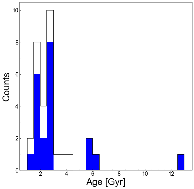
Figure 16: Age distribution of the 21 SCs identified in the LMC periphery, as examined in this work (depicted by the blue filled histogram). Additionally, we integrate data from 10 SCs previously analyzed in Gatto et al. (2020) with $G\geq$ 5 (represented by the black histogram).

Examining their fig. 5, we noticed that during the 1-1.58 Gyr interval (left-lower panel in their figure), the LMC star formation was more intense within the central bar, and in a morphological feature resembling a spiral arm that originates from the West edge of the bar and wraps to the North, encompassing the regions investigated by Pieres et al. (2016), in a counter-clockwise direction. At the greater look-back time, the SF is more evenly distributed around the LMC, with only the bar displaying a significantly more intense SF rate. Based on these observations, it seems plausible to infer that the region explored by Pieres et al. (2016) was undergoing an enhanced SC formation at about 1 Gyrs ago, while the LMC outskirts in other directions, including the fields analyzed in this work, were in a more quiescent phase, after a more intense SF activity occurred 2-3 Gyrs ago throughout the LMC, as also indicated by the secondary peak at 2.7 Gyrs identified by Pieres et al. (2016).

Even more importantly, as illustrated in Fig. 16, we confirm the existence of three reliable candidate SCs within the age gap, in particular having ages of 5.5-6.0 Gyr. Amongst them, we have already demonstrated (Gatto et al., 2022c) that KMHK 1762 (YMCA-0073) is the third ever confirmed age gap SC, besides ESO121-03 and KMHK 1592 (Piatti, 2022). The other two candidate SCs residing in the age-gap are YMCA-0053 and YMCA-0061. On these bases, and considering also the detailed discussion in Gatto et al. (2020), we shall conclude that the age gap in the SC population of the LMC, may either be significantly narrower than previously believed, lasting no more than 3 Gyr (e.g. between 7 - 10 Gyr), or it may be an artefact of the photometric and spatial limitations attained by the previous surveys. If confirmed, our results would fix the long-lasting debated issue about a different evolutionary path between SC and stellar field components in the LMC. We cannot exclude that low-mass SCs formed in the (now narrower) age gap were tidally disrupted (shocked) during the LMC-SMC encounter around 3 Gyr ago which thereby removed those clusters, whilst triggering the formation of new SCs around that time. This would allievate the cluster-field tension also.

In order to confirm the reality of the newly discovered SC candidates, especially those within the age gap, further photometric follow-up is necessary. Indeed, given that the new SC candidates are generally old and faint, very deep photometry, up to four magnitudes below the MSTO (i.e. $V\sim$ 26.5 mag) obtained in very good seeing conditions (to reduce confusion) would be valuable to confirm them as real physical systems. The advent of the Rubin-LSST telescope is expected to greatly aid in this endeavour, as it promises to deliver deep photometry across the entire southern sky, and has a dedicated observational program for the MCs (Olsen et al., 2018).

6.6 Density profiles

To estimate the structural parameters of the SCs under investigation we derived their radial density profiles (RDP) and we fitted them with the Elson, Fall, and Freeman (EFF; Elson et al., 1987) profile:

$$n(r)=n_{0}\times\left(1+\frac{r^{2}}{\alpha^{2}}\right)^{\frac{-\gamma}{2}}+\phi$$ (3)

where $n(r)$ represents the number of stars per squared arcminute as a function of the distance from the centre of the cluster, $n_{0}$ is the central surface density, $\alpha$ is the core parameter, $\gamma$ is the slope parameter, and $\phi$ is the background value, which is a free parameter of the fit. We obtained the best fitting parameters through the module curve fit of the Python library scipy. These parameters can be used to calculate the core radius of the SCs using the equation:

$$r_{c}=\alpha\times\sqrt{2^{2/\gamma}-1}$$ (4)

We inserted the values of $n_{0}$ and the core radius for each SC in both arcminute and parsec in Table 6 (columns eight to ten). To obtain the physical size of the core radius, we applied a correction for the adopted distance modulus of the LMC or the SMC, depending on the SC membership. Figures 21 and 23 display the RDPs and their best fit profile for the known SCs analyzed in this work, and for the new candidate SCs, respectively.

7 Summary

We have presented and discussed the data acquired with the YMCA survey, a wide-field optical imaging project conducted with the VLT Survey Telescope using $g$ and $i$ filters. The primary objective of YMCA is to reconstruct the evolution of the MCs and unravel their complex interaction history. It covers 110 square degrees in the periphery of both the MCs. Specifically, this survey covered the East and West side of the LMC, the North-West side of the SMC, and a strip of 1° in size above the Magellanic Bridge that links the two Clouds. These targeted regions complement the optical STEP survey, which probed the main body of the SMC and the Bridge, utilizing the same instrument and with similar observing constraints. Together, YMCA and STEP provide a deep catalogue covering more than 160 square degrees within the Magellanic System. The YMCA catalog of stars adopted in this work will be published at the CDS.

The depth and accuracy achieved by YMCA allows us to resolve individual stars down to $\simeq$ 1.5-2.0 mag below the MSTO of the oldest stellar population of the MCs, opening a view into the early stages of their evolution. While preliminary studies based on subsamples of the YMCA catalogue already demonstrated the potential of this survey in addressing critical questions about the past MCs’ evolutionary path (Gatto et al., 2020, 2021, 2022c), here we presented an overall analysis of the stellar field population within the periphery of the MCs, including their SC system, by leveraging the full YMCA dataset.

The analysis of the deep CMD constructed with the YMCA photometric catalogue suggests:

• The peripheries of the LMC and the SMC are dominated by intermediate-age and old stellar populations. This finding is common amongst star-forming dwarf galaxies in the Local Group. (see the review by Annibali & Tosi, 2022, and references therein)

• While the North-West side of the SMC does not exhibit the presence of young stars, a moderate blue plume, indicating a younger (t $\sim$ 300 - 500 Myr) stellar population is evident within the YMCA tiles closest to the LMC, on both its West and East sides. Notably, the tile 7_27, situated near the West edge of the LMC bar, shows a more pronounced blue plume, suggesting that a more recent event (t $\simeq$ 200 Myr) of star formation may have occurred.

• Consistently with observations by Mackey et al. (2018), the LMC disc appears to be truncated on its Western side at about $9\degr$, namely 8 kpc from the LMC centre. This feature might be the consequence of a close encounter with the SMC (Belokurov & Erkal, 2019).

• We confirmed the presence of a foreground stellar population, hinted by the presence of a double RC in the CMD, towards the North-Eastern direction of the SMC (see also Omkumar et al., 2021; James et al., 2021). The closer substructure emerges at $\simeq 2.8\degree$ from the SMC centre, and is clearly visible up to $\simeq 5.5\degree$, in line with previous studies (Omkumar et al., 2021).

In addition, we investigated SCs properties within the YMCA footprint to get additional insights into the MCs’ past evolution. This pursuit involved an in-depth analysis of SCs properties already documented in the literature by means of the deeper YMCA survey, as well as an extensive research to detect unknown SCs adopting a customized algorithm applied to the YMCA dataset. In particular:

• We detected 9 new candidate SCs in the outskirts of the LMC.

• In agreement with previous studies, the age distribution of the SCs showcases a pronounced peak at $\simeq$ 2–3 Gyr. This finding potentially sheds light on the timeline of a past close encounter between the LMC and the SMC, the likely main actor of such a sudden increase in the SC formation activity.

• The age distribution of the SCs examined in this work challenges the actual existence of the so-called age gap in the LMC, proposed more than three decades ago (Jensen et al., 1988; Da Costa, 1991), and already questioned in Gatto et al. (2020) and in Gatto et al. (2022c).

Deeper photometric follow-ups are crucial to confirm the existence of a population of SCs born during the age-gap period, and thus to finally resolve the long-standing debated discrepancy between the star field and SC formation histories observed in this broad period of the LMC lifetime.

Appendix A Age comparison with literature

As a crucial validation step of the procedure described in Sect. 6.3, we undertook a comparative analysis of the estimated ages for SCs derived using our visual fitting procedure with those available in literature. This was done to ensure that fixing two parameters, namely distance modulus and metallicity, did not introduce any bias into the age assessment process. Specifically, we identified 16 SCs (comprising 3 in the vicinity of SMC, 1 within the studied Strip, and the remaining 12 in the outskirts of the LMC), all of which had been previously documented in various works (refer to Section 6.4 for details). Among these 16 SCs, age values were successfully retrieved for 10 of them. Therefore, for 6 SCs that were already known we provide for the first time their age estimations. It is noteworthy that KMHK1762 was excluded from the analysis of the aforementioned 10 SCs, as in a dedicated study (Gatto et al. 2022c), we demonstrated that, considering the fainter limiting magnitude of the YMCA dataset, KMHK 1762 is significantly older than previously thought.

Table 7 displays the list of SCs with ages reported in literature and their references. Figure 17 illustrates the comparison between the ages determined through our visual isochrone matching and those obtained from prior studies for 9 SCs (6 located in the outskirts of the LMC and 3 in the periphery of the SMC). Importantly, the age values for these 9 SCs were sourced from five distinct works (see caption of the figure). Moreover the age estimations were derived using diverse methodologies, resulting in a highly heterogeneous dataset. Nevertheless, the plot reveals a good agreement with respect to the literature’s age estimations, with a mean difference of $\log(t_{\rm our})-\log(t_{\rm lit})$ = -0.005 dex, as indicated by the blue line in the figure. All SC age estimations are consistent within their errors when compared to values provided by other works. Notably, this agreement does not exhibit any discernible trend with age. This finding indicates that YMCA photometry is sufficiently accurate even at faint magnitudes to allow us to visually identify the actual magnitude of the MSTO of these SCs. In light of these considerations, we assert our confidence that the steps taken in our isochrone matching procedure did not introduce any significant effect on the determination of SC ages.

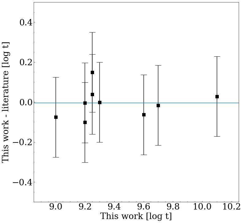
Figure 17: Age difference between this work and literature values as a function of the age estimated in this work. The horizontal blue line indicates the mean of the difference, which is $\log(t_{\rm our})-\log(t_{\rm lit})$ = -0.005 dex. Errorbars on the y-axis represent our estimated uncertainties, namely $\sigma_{\log t}=0.2$ dex. Literature values have been taken from Parisi et al. (2014), Piatti & Bastian (2016), Piatti et al. (2018), Maia et al. (2019), and Milone et al. (2023).

Table 7: Comparison between the SC ages estimated in this work and literature values.

ID	$\log t$ (Our)	$\log t$ (Lit.)	Reference	Simbad Name
YMCA-0049	9.60	$9.66\pm 0.02$	1	L 32
YMCA-0050	9.70	$9.72\pm 0.04$	1	ESO 51-9
YMCA-0051	9.20	$9.20\pm 0.05$	1	HW 84
YMCA-0056	9.25	$9.10\pm 0.10$	2	KMHK 5
YMCA-0058	9.30	$9.30\pm 0.10$	2	KMHK 11
YMCA-0059	9.25	$9.21\pm 0.05$	3	NGC 1644
YMCA-0065	9.20	$9.30\pm 0.02$	4	KMHK 1751
YMCA-0070	10.10	$10.07\pm 0.02$	3	NGC 2257
YMCA-0072	9.00	$9.08\pm 0.05$	5	KMHK 1760

Appendix B CMD of SCs in the MC periphery

In this section we present the CMDs of all SCs analyzed in this work, a comparison with the CMD of the local stellar field, and the relative spatial distribution of their star with respect to their estimated centre. In particular, in Fig. 18 we show these plots for the SCs already reported in the literature, whereas Fig. 20 displays the same subplots for the candidate SCs discussed in this work.

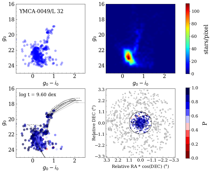
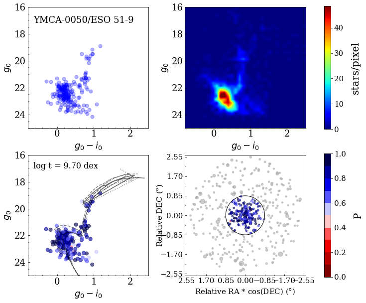
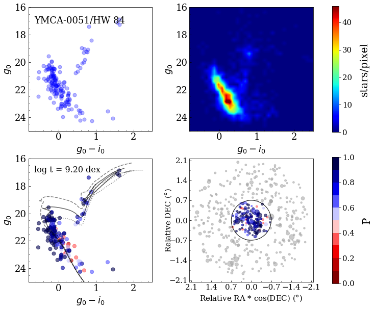
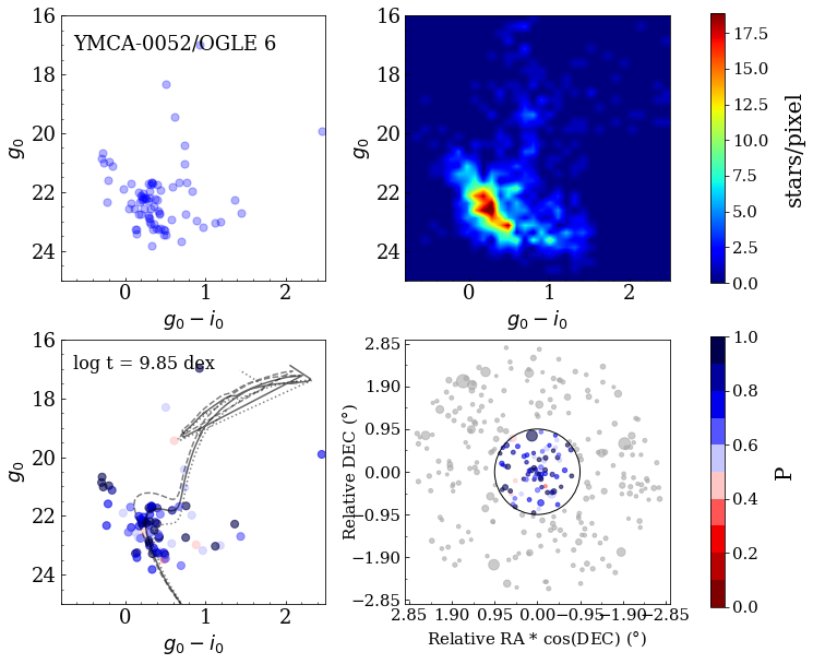
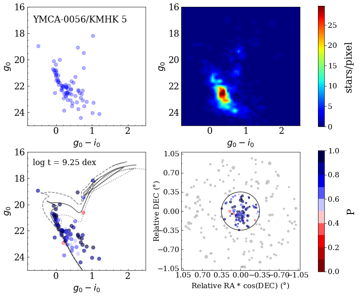
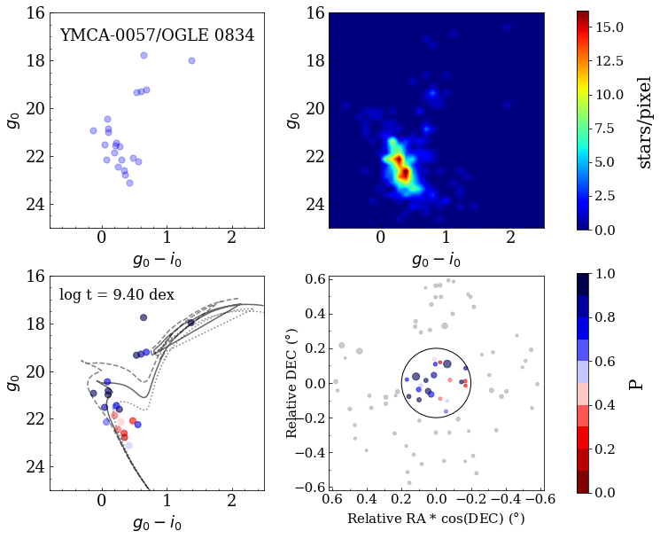
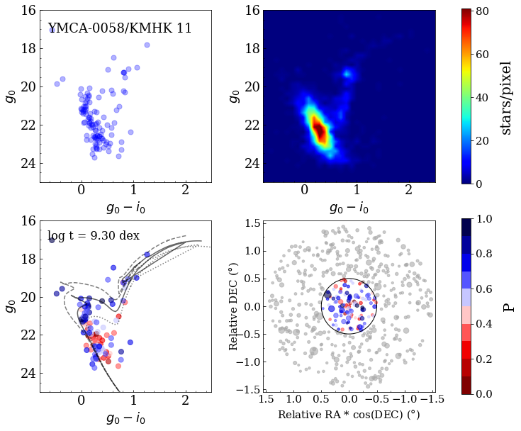
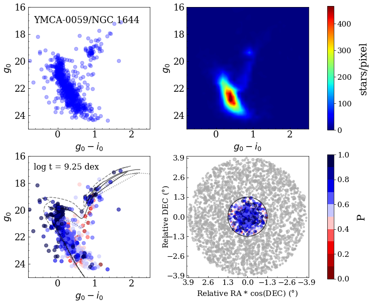
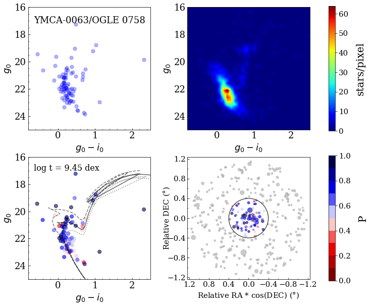
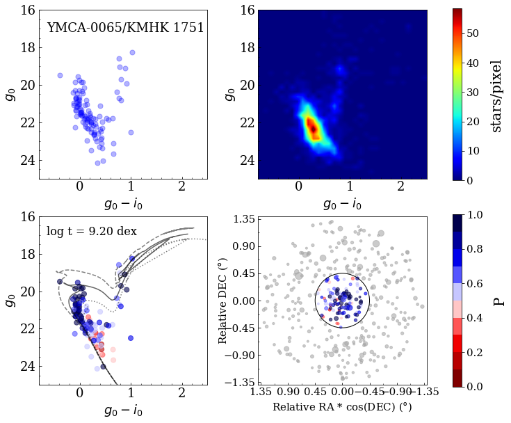
Figure 18: SCs already known analyzed in this work. For each of them this figure illustrates: Top Left: CMD of the candidate SC; Top Right: Hess diagram of the six fields used as representative of the local stellar field contamination; Bottom Left: CMD of the SC with stars colour coded according to their membership probability of being a cluster member along with the best fitting isochrone (solid line) and isochrones at log(t) = $\pm$0.2 dex from the best one; Bottom Right: Spatial distribution of stars with respect to the SC centre. The solid circle marks the estimated SC radius.

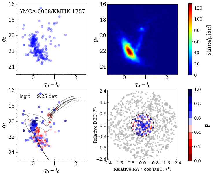
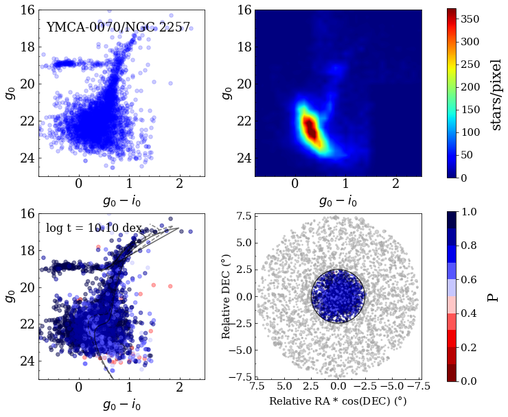
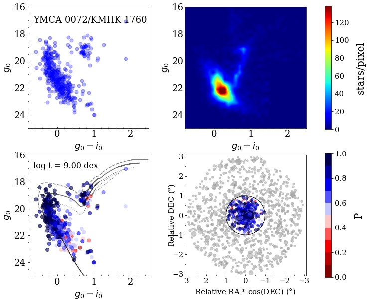
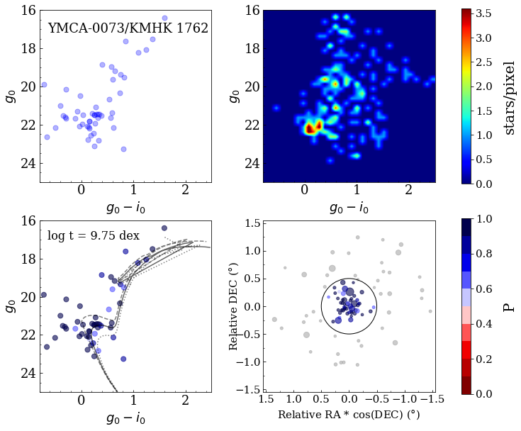
Figure 19: Continued

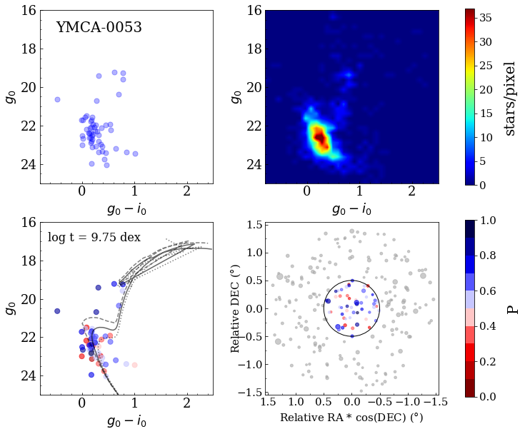
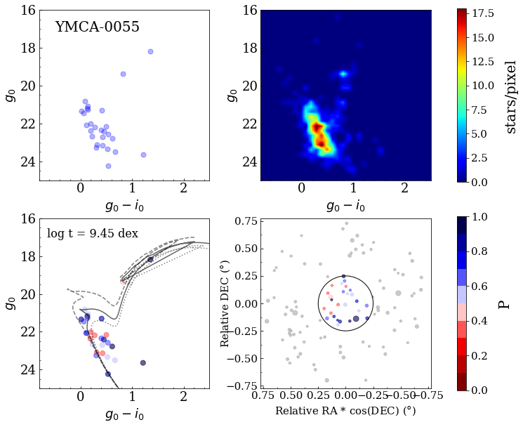
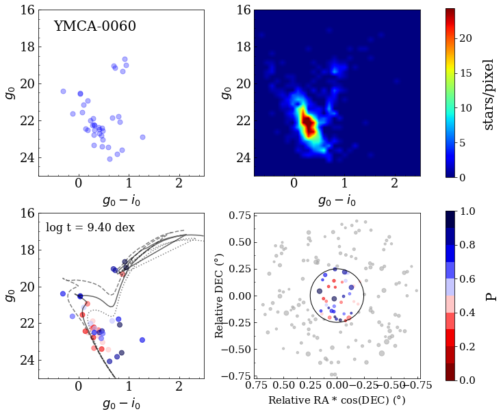
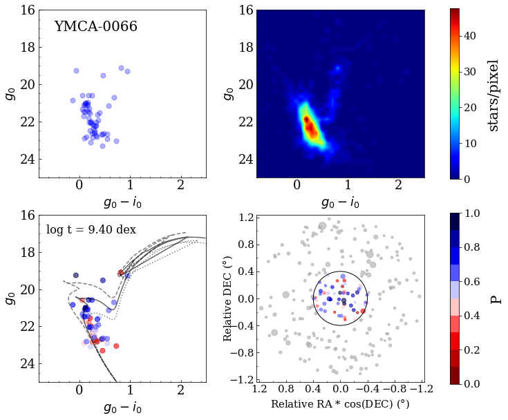
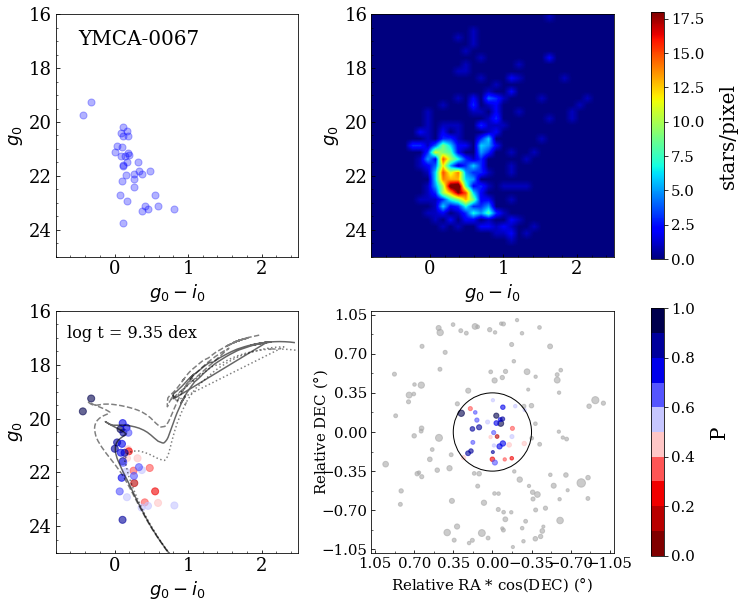
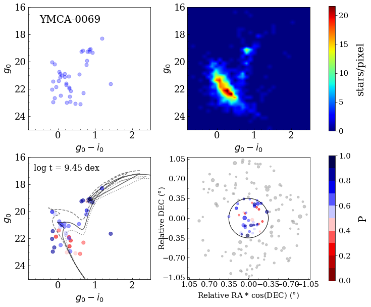
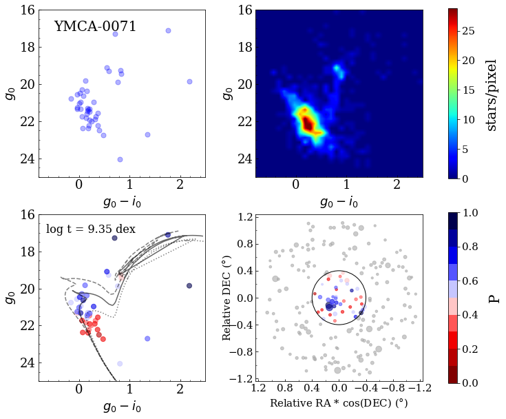
Figure 20: Same as Figure 18, but for the new candidate SCs.

Appendix C Radial density profile of SCs in the MC periphery

In this section we present the RDPs and their best fit EFF profile for all SCs analyzed in this work. In Fig. 21 we show the RDPs for the SCs already reported in literature, whereas Fig. 23 displays the RDPs for the candidate SCs discussed in this work.

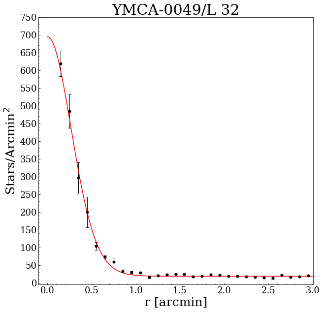
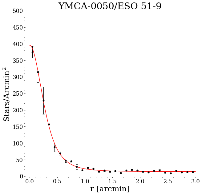
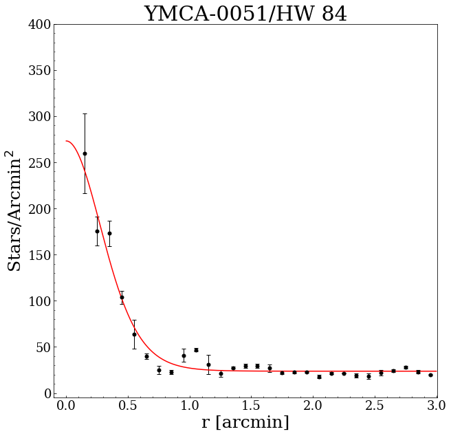
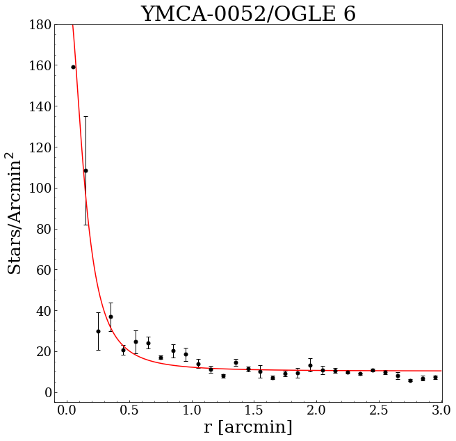
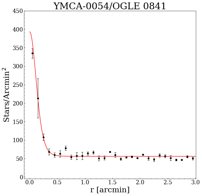
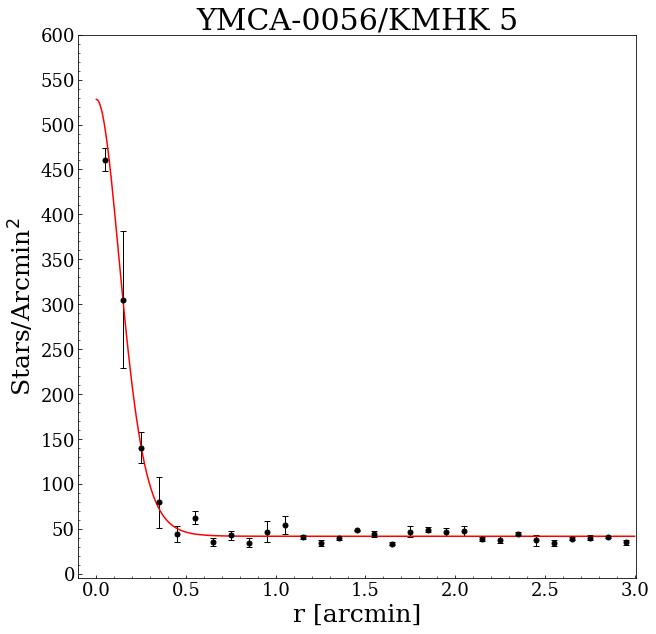
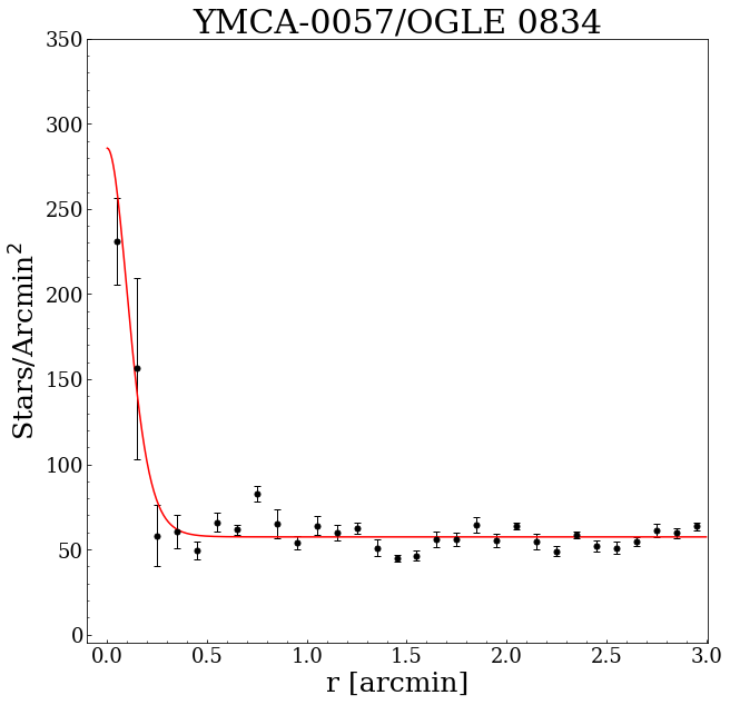
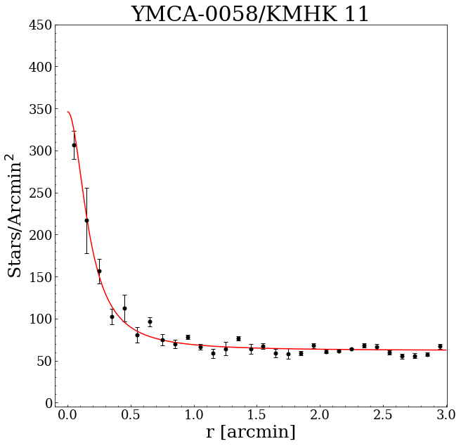
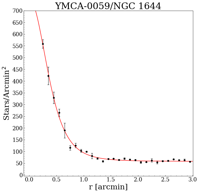
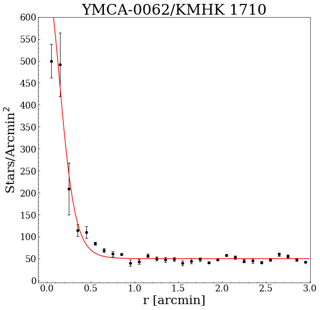
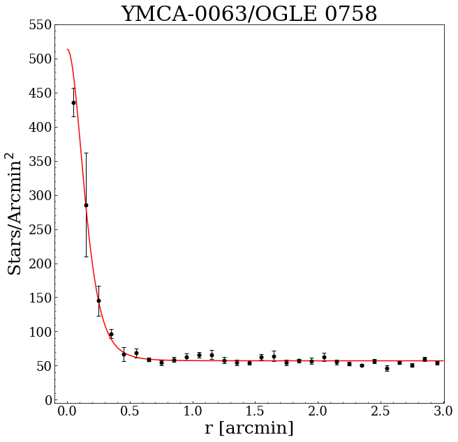
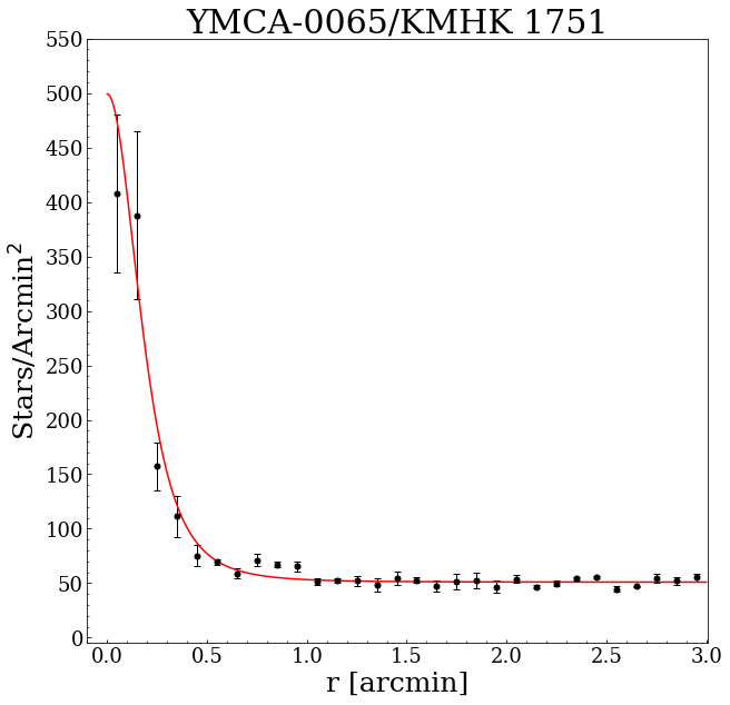
Figure 21: RDPs for all SCs already known. The red solid line indicates the best EFF profile (see Sect. 6.6 for the description of the fit procedure).

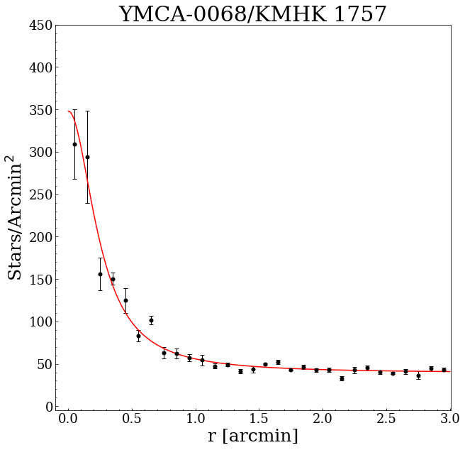
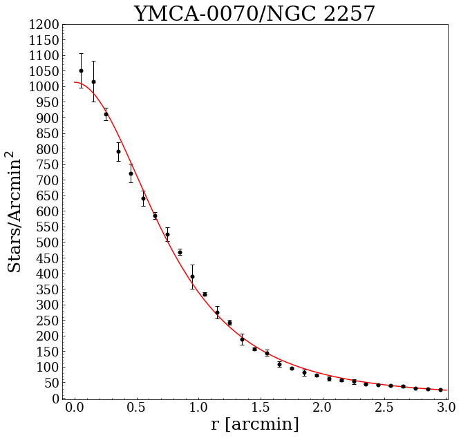
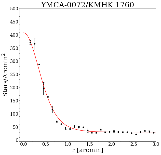
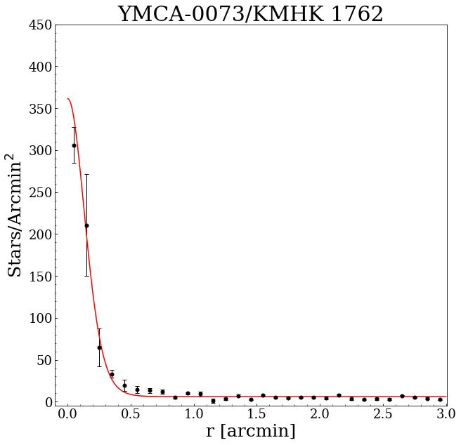
Figure 22: Continued

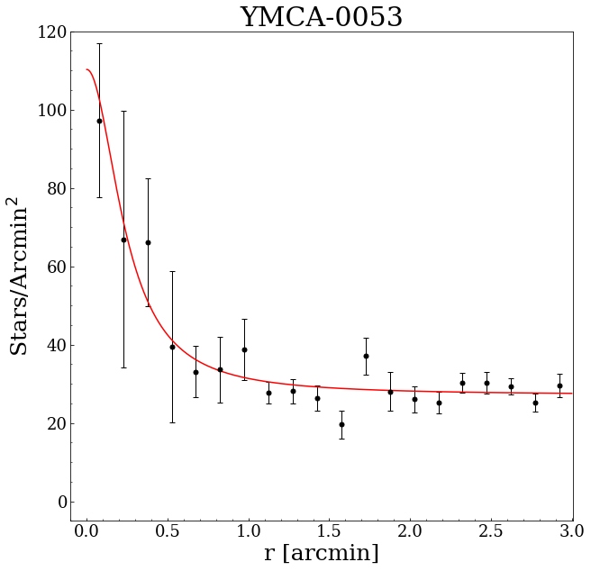
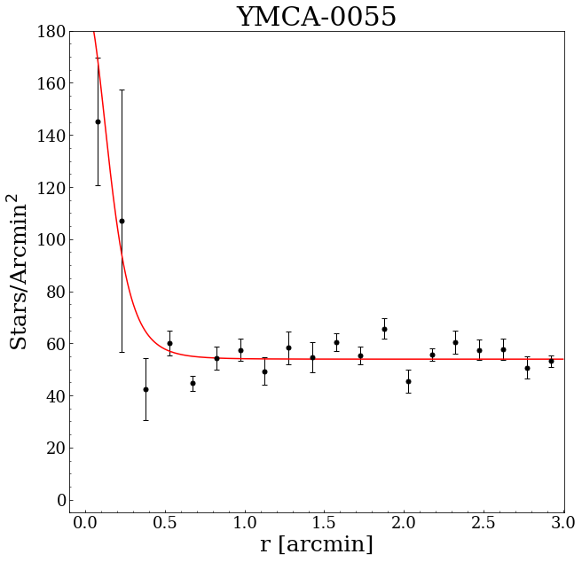
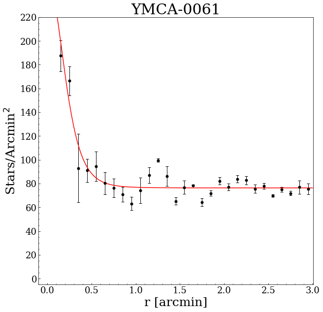
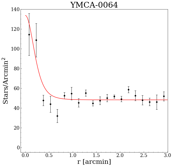
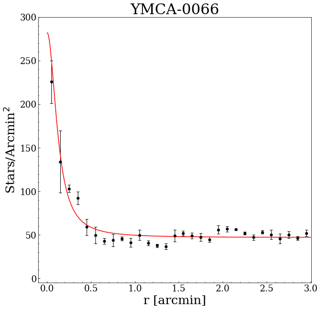
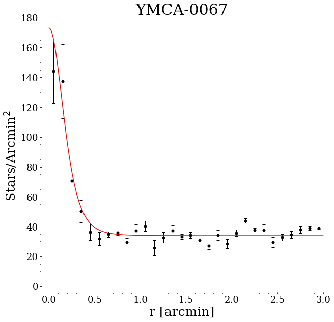
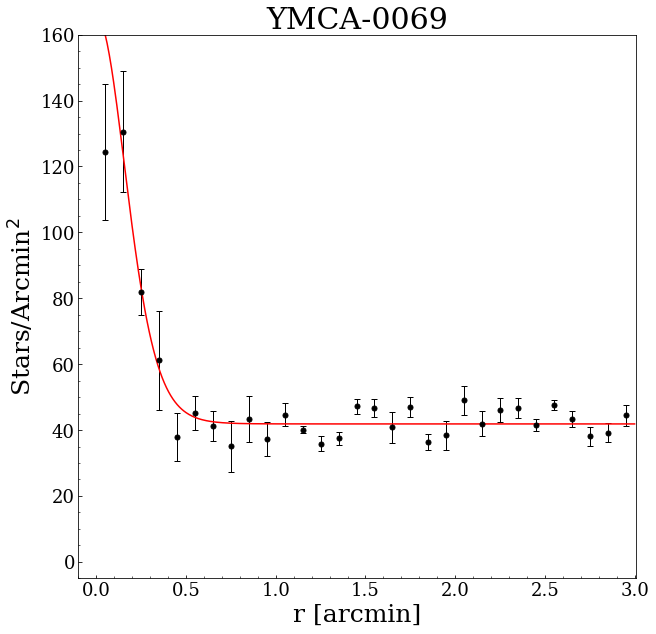
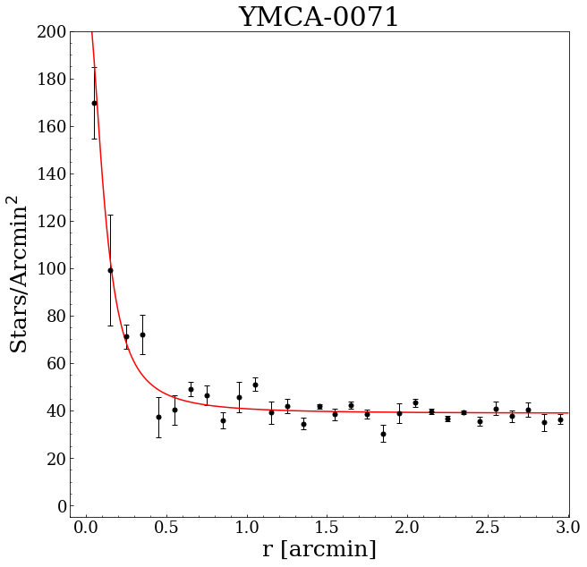
Figure 23: Same as Figure 21, but for the new candidate SCs.

References

- Amorisco et al. (2014) Amorisco, N. C., Evans, N. W., & van de Ven, G. 2014, Nature, 507, 335
- Annibali et al. (2016) Annibali, F., Nipoti, C., Ciotti, L., et al. 2016, ApJ, 826, L27
- Annibali & Tosi (2022) Annibali, F. & Tosi, M. 2022, Nature Astronomy, 6, 48
- Bagheri et al. (2013) Bagheri, G., Cioni, M. R. L., & Napiwotzki, R. 2013, A&A, 551, A78
- Bekki & Chiba (2005) Bekki, K. & Chiba, M. 2005, MNRAS, 356, 680
- Belokurov & Koposov (2016) Belokurov, V. & Koposov, S. E. 2016, MNRAS, 456, 602
- Belokurov & Erkal (2019) Belokurov, V. A. & Erkal, D. 2019, MNRAS, 482, L9
- Bertin & Arnouts (1996) Bertin, E. & Arnouts, S. 1996, A&AS, 117, 393
- Besla et al. (2012) Besla, G., Kallivayalil, N., Hernquist, L., et al. 2012, MNRAS, 421, 2109
- Bica et al. (2008) Bica, E., Bonatto, C., Dutra, C. M., & Santos, J. F. 2008, Monthly Notices of the Royal Astronomical Society, 389, 678
- Bressan et al. (2012) Bressan, A., Marigo, P., Girardi, L., et al. 2012, MNRAS, 427, 127
- Brocato et al. (2003) Brocato, E., Castellani, V., Di Carlo, E., Raimondo, G., & Walker, A. R. 2003, AJ, 125, 3111
- Brüns et al. (2005) Brüns, C., Kerp, J., Staveley-Smith, L., et al. 2005, A&A, 432, 45
- Bullock & Johnston (2005) Bullock, J. S. & Johnston, K. V. 2005, ApJ, 635, 931
- Capaccioli & Schipani (2011) Capaccioli, M. & Schipani, P. 2011, The Messenger, 146, 2
- Capaccioli et al. (2015) Capaccioli, M., Spavone, M., Grado, A., et al. 2015, A&A, 581, A10
- Carrera et al. (2017) Carrera, R., Conn, B. C., Noël, N. E. D., Read, J. I., & López Sánchez, Á. R. 2017, MNRAS, 471, 4571
- Cerny et al. (2021) Cerny, W., Pace, A. B., Drlica-Wagner, A., et al. 2021, ApJ, 910, 18
- Chandra et al. (2023) Chandra, V., Naidu, R. P., Conroy, C., et al. 2023, ApJ, 956, 110
- Choi et al. (2018) Choi, Y., Nidever, D. L., Olsen, K., et al. 2018, ApJ, 869, 125
- Choi et al. (2022) Choi, Y., Olsen, K. A. G., Besla, G., et al. 2022, ApJ, 927, 153
- Cignoni et al. (2013) Cignoni, M., Cole, A. A., Tosi, M., et al. 2013, ApJ, 775, 83
- Cioni et al. (2011) Cioni, M. R. L., Clementini, G., Girardi, L., et al. 2011, A&A, 527, A116
- Cooper et al. (2010) Cooper, A., Cole, S., Frenk, C., et al. 2010, Monthly notices of the royal astronomical society, 406, 744
- Cooper et al. (2015) Cooper, A. P., Gao, L., Guo, Q., et al. 2015, MNRAS, 451, 2703
- Da Costa (1991) Da Costa, G. S. 1991, in IAU Symposium, Vol. 148, The Magellanic Clouds, ed. R. Haynes & D. Milne, 183
- Dark Energy Survey Collaboration et al. (2016) Dark Energy Survey Collaboration, Abbott, T., Abdalla, F. B., et al. 2016, MNRAS, 460, 1270
- de Grijs & Bono (2015) de Grijs, R. & Bono, G. 2015, AJ, 149, 179
- Deason et al. (2014) Deason, A. J., Belokurov, V., Koposov, S. E., & Rockosi, C. M. 2014, ApJ, 787, 30
- Demers & Battinelli (1998) Demers, S. & Battinelli, P. 1998, AJ, 115, 154
- Dobbie et al. (2014) Dobbie, P. D., Cole, A. A., Subramaniam, A., & Keller, S. 2014, MNRAS, 442, 1663
- D’Onghia & Fox (2016) D’Onghia, E. & Fox, A. J. 2016, ARA&A, 54, 363
- Drlica-Wagner et al. (2016) Drlica-Wagner, A., Bechtol, K., Allam, S., et al. 2016, ApJ, 833, L5
- El Youssoufi et al. (2021) El Youssoufi, D., Cioni, M.-R. L., Bell, C. P. M., et al. 2021, MNRAS, 505, 2020
- Elson et al. (1987) Elson, R. A. W., Fall, S. M., & Freeman, K. C. 1987, ApJ, 323, 54
- Gaia Collaboration et al. (2018) Gaia Collaboration, Brown, A. G. A., Vallenari, A., et al. 2018, A&A, 616, A1
- Gaia Collaboration et al. (2021) Gaia Collaboration, Luri, X., Chemin, L., et al. 2021, A&A, 649, A7
- Gaia Collaboration et al. (2023) Gaia Collaboration, Montegriffo, P., Bellazzini, M., et al. 2023, A&A, 674, A33
- Gatto et al. (2020) Gatto, M., Ripepi, V., Bellazzini, M., et al. 2020, MNRAS, 499, 4114
- Gatto et al. (2022a) Gatto, M., Ripepi, V., Bellazzini, M., et al. 2022a, ApJ, 929, L21
- Gatto et al. (2022b) Gatto, M., Ripepi, V., Bellazzini, M., et al. 2022b, ApJ, 931, 19
- Gatto et al. (2022c) Gatto, M., Ripepi, V., Bellazzini, M., et al. 2022c, A&A, 664, L12
- Gatto et al. (2021) Gatto, M., Ripepi, V., Bellazzini, M., et al. 2021, Research Notes of the American Astronomical Society, 5, 159
- Girardi (2016) Girardi, L. 2016, ARA&A, 54, 95
- Girardi & Marigo (2007) Girardi, L. & Marigo, P. 2007, A&A, 462, 237
- Girardi & Salaris (2001) Girardi, L. & Salaris, M. 2001, MNRAS, 323, 109
- Grado et al. (2012) Grado, A., Capaccioli, M., Limatola, L., & Getman, F. 2012, Memorie della Societa Astronomica Italiana Supplementi, 19, 362
- Green (2018) Green, G. 2018, The Journal of Open Source Software, 3, 695
- Harris et al. (2020) Harris, C. R., Millman, K. J., van der Walt, S. J., et al. 2020, Nature, 585, 357
- Harris (2007) Harris, J. 2007, ApJ, 658, 345
- Harris & Zaritsky (2009) Harris, J. & Zaritsky, D. 2009, Astronomical Journal, 138, 1243
- Hindman et al. (1963) Hindman, J. V., Kerr, F. J., & McGee, R. X. 1963, Australian Journal of Physics, 16, 570
- Hunter (2007) Hunter, J. D. 2007, Computing in Science & Engineering, 9, 90
- Indu & Subramaniam (2011) Indu, G. & Subramaniam, A. 2011, A&A, 535, A115
- Irwin et al. (1985) Irwin, M. J., Kunkel, W. E., & Demers, S. 1985, Nature, 318, 160
- James et al. (2021) James, D., Subramanian, S., Omkumar, A. O., et al. 2021, MNRAS, 508, 5854
- Jensen et al. (1988) Jensen, J., Mould, J., & Reid, N. 1988, ApJS, 67, 77
- Kallivayalil et al. (2018) Kallivayalil, N., Sales, L. V., Zivick, P., et al. 2018, ApJ, 867, 19
- Kallivayalil et al. (2006) Kallivayalil, N., van der Marel, R. P., Alcock, C., et al. 2006, ApJ, 638, 772
- Kallivayalil et al. (2013) Kallivayalil, N., van der Marel, R. P., Besla, G., Anderson, J., & Alcock, C. 2013, ApJ, 764, 161
- Keller & Wood (2002) Keller, S. C. & Wood, P. R. 2002, ApJ, 578, 144
- Keller & Wood (2006) Keller, S. C. & Wood, P. R. 2006, ApJ, 642, 834
- Koposov et al. (2015) Koposov, S. E., Belokurov, V., Torrealba, G., & Evans, N. W. 2015, ApJ, 805, 130
- Koposov et al. (2018) Koposov, S. E., Walker, M. G., Belokurov, V., et al. 2018, MNRAS, 479, 5343
- Kuijken (2011) Kuijken, K. 2011, The Messenger, 146, 8
- Lebzelter & Wood (2007) Lebzelter, T. & Wood, P. R. 2007, A&A, 475, 643
- Lynden-Bell (1976) Lynden-Bell, D. 1976, MNRAS, 174, 695
- Mackey et al. (2017) Mackey, A. D., Koposov, S. E., Da Costa, G. S., et al. 2017, MNRAS, 472, 2975
- Mackey et al. (2016) Mackey, A. D., Koposov, S. E., Erkal, D., et al. 2016, MNRAS, 459, 239
- Mackey et al. (2018) Mackey, D., Koposov, S., Da Costa, G., et al. 2018, ApJ, 858, L21
- Maia et al. (2019) Maia, F. F. S., Dias, B., Santos, J. F. C., et al. 2019, MNRAS, 484, 5702
- Marconi & Clementini (2005) Marconi, M. & Clementini, G. 2005, AJ, 129, 2257
- Marconi et al. (2017) Marconi, M., Molinaro, R., Ripepi, V., et al. 2017, MNRAS, 466, 3206
- Martin et al. (2015) Martin, N. F., Nidever, D. L., Besla, G., et al. 2015, ApJ, 804, L5
- Massana et al. (2020) Massana, P., Noël, N. E. D., Nidever, D. L., et al. 2020, MNRAS, 498, 1034
- Massana et al. (2022) Massana, P., Ruiz-Lara, T., Noël, N. E. D., et al. 2022, MNRAS, 513, L40
- Mathewson et al. (1974) Mathewson, D. S., Cleary, M. N., & Murray, J. D. 1974, ApJ, 190, 291
- Mazzi et al. (2021) Mazzi, A., Girardi, L., Zaggia, S., et al. 2021, MNRAS, 508, 245
- McFarland et al. (2013) McFarland, J. P., Verdoes-Kleijn, G., Sikkema, G., et al. 2013, Experimental Astronomy, 35, 45
- Milone et al. (2023) Milone, A. P., Cordoni, G., Marino, A. F., et al. 2023, A&A, 672, A161
- Muñoz et al. (2006) Muñoz, R. R., Majewski, S. R., Zaggia, S., et al. 2006, ApJ, 649, 201
- Newville et al. (2014) Newville, M., Stensitzki, T., Allen, D. B., & Ingargiola, A. 2014, LMFIT: Non-Linear Least-Square Minimization and Curve-Fitting for Python
- Nidever et al. (2010) Nidever, D. L., Majewski, S. R., Butler Burton, W., & Nigra, L. 2010, ApJ, 723, 1618
- Nidever et al. (2013) Nidever, D. L., Monachesi, A., Bell, E. F., et al. 2013, ApJ, 779, 145
- Nidever et al. (2019) Nidever, D. L., Olsen, K., Choi, Y., et al. 2019, ApJ, 874, 118
- Nidever et al. (2017) Nidever, D. L., Olsen, K., Walker, A. R., et al. 2017, AJ, 154, 199
- Noël et al. (2013) Noël, N. E. D., Conn, B. C., Carrera, R., et al. 2013, ApJ, 768, 109
- Noël et al. (2015) Noël, N. E. D., Conn, B. C., Read, J. I., et al. 2015, MNRAS, 452, 4222
- Olsen et al. (2018) Olsen, K., Szkody, P., Cioni, M.-R., et al. 2018, arXiv e-prints, arXiv:1812.03139
- Omkumar et al. (2021) Omkumar, A. O., Subramanian, S., Niederhofer, F., et al. 2021, MNRAS, 500, 2757
- Pace & Li (2019) Pace, A. B. & Li, T. S. 2019, ApJ, 875, 77
- pandas development team (2020) pandas development team, T. 2020, pandas-dev/pandas: Pandas
- Pardy et al. (2020) Pardy, S. A., D’Onghia, E., Navarro, J. F., et al. 2020, MNRAS, 492, 1543
- Parisi et al. (2014) Parisi, M. C., Geisler, D., Carraro, G., et al. 2014, AJ, 147, 71
- Parisi et al. (2015) Parisi, M. C., Geisler, D., Clariá, J. J., et al. 2015, AJ, 149, 154
- Patel et al. (2020) Patel, E., Kallivayalil, N., Garavito-Camargo, N., et al. 2020, ApJ, 893, 121
- Pedregosa et al. (2011) Pedregosa, F., Varoquaux, G., Gramfort, A., et al. 2011, Journal of Machine Learning Research, 12, 2825
- Petersen et al. (2022) Petersen, M. S., Peñarrubia, J., & Jones, E. 2022, MNRAS, 514, 1266
- Piatti (2022) Piatti, A. E. 2022, MNRAS, 511, L72
- Piatti & Bastian (2016) Piatti, A. E. & Bastian, N. 2016, A&A, 590, A50
- Piatti & Bica (2012) Piatti, A. E. & Bica, E. 2012, Monthly Notices of the Royal Astronomical Society, 425, 3085
- Piatti et al. (2018) Piatti, A. E., Cole, A. A., & Emptage, B. 2018, Monthly Notices of the Royal Astronomical Society, 473, 105
- Piatti & Geisler (2013) Piatti, A. E. & Geisler, D. 2013, Astronomical Journal, 145
- Pieres et al. (2016) Pieres, A., Santiago, B., Balbinot, E., et al. 2016, MNRAS, 461, 519
- Pieres et al. (2017) Pieres, A., Santiago, B. X., Drlica-Wagner, A., et al. 2017, MNRAS, 468, 1349
- Pietrzyński et al. (2019) Pietrzyński, G., Graczyk, D., Gallenne, A., et al. 2019, Nature, 567, 200
- Price-Whelan et al. (2019) Price-Whelan, A. M., Nidever, D. L., Choi, Y., et al. 2019, ApJ, 887, 19
- Putman et al. (1998) Putman, M. E., Gibson, B. K., Staveley-Smith, L., et al. 1998, Nature, 394, 752
- Putman et al. (2003) Putman, M. E., Staveley-Smith, L., Freeman, K. C., Gibson, B. K., & Barnes, D. G. 2003, ApJ, 586, 170
- Rezaeikh et al. (2014) Rezaeikh, S., Javadi, A., Khosroshahi, H., & van Loon, J. T. 2014, MNRAS, 445, 2214
- Riess et al. (2021) Riess, A. G., Casertano, S., Yuan, W., et al. 2021, ApJ, 908, L6
- Ripepi et al. (2021) Ripepi, V., Catanzaro, G., Molinaro, R., et al. 2021, MNRAS, 508, 4047
- Ripepi et al. (2022) Ripepi, V., Chemin, L., Molinaro, R., et al. 2022, MNRAS, 512, 563
- Ripepi et al. (2014) Ripepi, V., Cignoni, M., Tosi, M., et al. 2014, MNRAS, 442, 1897
- Rubele et al. (2018) Rubele, S., Pastorelli, G., Girardi, L., et al. 2018, MNRAS, 478, 5017
- Saha et al. (2010) Saha, A., Olszewski, E. W., Brondel, B., et al. 2010, AJ, 140, 1719
- Schlafly & Finkbeiner (2011) Schlafly, E. F. & Finkbeiner, D. P. 2011, ApJ, 737, 103
- Schlegel et al. (1998) Schlegel, D. J., Finkbeiner, D. P., & Davis, M. 1998, ApJ, 500, 525
- Schmidt et al. (2020) Schmidt, T., Cioni, M.-R. L., Niederhofer, F., et al. 2020, A&A, 641, A134
- Skowron et al. (2014) Skowron, D. M., Jacyszyn, A. M., Udalski, A., et al. 2014, ApJ, 795, 108
- Skowron et al. (2021) Skowron, D. M., Skowron, J., Udalski, A., et al. 2021, ApJS, 252, 23
- Stetson (1987) Stetson, P. B. 1987, PASP, 99, 191
- Stetson (1992) Stetson, P. B. 1992, Astronomical Society of the Pacific Conference Series, Vol. 25, More Experiments with DAOPHOT II and WF/PC Images, ed. D. M. Worrall, C. Biemesderfer, & J. Barnes, 297
- Subramanian et al. (2017) Subramanian, S., Rubele, S., Sun, N.-C., et al. 2017, MNRAS, 467, 2980
- Tatton et al. (2021) Tatton, B. L., van Loon, J. T., Cioni, M. R. L., et al. 2021, MNRAS, 504, 2983
- Taylor (2005) Taylor, M. B. 2005, in Astronomical Society of the Pacific Conference Series, Vol. 347, Astronomical Data Analysis Software and Systems XIV, ed. P. Shopbell, M. Britton, & R. Ebert, 29
- Taylor (2006) Taylor, M. B. 2006, in Astronomical Society of the Pacific Conference Series, Vol. 351, Astronomical Data Analysis Software and Systems XV, ed. C. Gabriel, C. Arviset, D. Ponz, & S. Enrique, 666
- Torrealba et al. (2018) Torrealba, G., Belokurov, V., Koposov, S. E., et al. 2018, MNRAS, 475, 5085
- Udalski et al. (2015) Udalski, A., Szymański, M. K., & Szymański, G. 2015, Acta Astron., 65, 1
- Vasiliev (2024) Vasiliev, E. 2024, MNRAS, 527, 437
- Wes McKinney (2010) Wes McKinney. 2010, in Proceedings of the 9th Python in Science Conference, ed. Stéfan van der Walt & Jarrod Millman, 56 – 61
- Zaritsky et al. (2020) Zaritsky, D., Conroy, C., Naidu, R. P., et al. 2020, ApJ, 905, L3
- Zivick et al. (2019) Zivick, P., Kallivayalil, N., Besla, G., et al. 2019, ApJ, 874, 78
- Zivick et al. (2018) Zivick, P., Kallivayalil, N., van der Marel, R. P., et al. 2018, ApJ, 864, 55